the Creative Commons Attribution 4.0 License.
the Creative Commons Attribution 4.0 License.
 | 04 Aug 2023
Sensitivity of gyre-scale marine connectivity estimates to fine-scale circulation
Saeed Hariri
Sabrina Speich
Bruno Blanke
Marina Lévy
We investigated the connectivity properties of an idealized western boundary current system separating two ocean gyres, where the flow is characterized by a well-defined mean circulation as well as energetic fine-scale features (i.e., mesoscale and submesoscale currents). We used a time-evolving 3D flow field from a high-resolution (HR-3D) ocean model of this system. In order to evaluate the role of the fine scales in connectivity estimates, we computed Lagrangian trajectories in three different ways: using the HR-3D flow, using the same flow but filtered on a coarse-resolution grid (CR-3D), and using the surface layer flow only (HR-SL). We examined connectivity between the two gyres along the western boundary current and across it by using and comparing different metrics, such as minimum and averaged values of transit time between 16 key sites, arrival depths, and probability density functions of transit times. We find that when the fine-scale flow is resolved, the numerical particles connect pairs of sites faster (between 100 to 300 d) than when it is absent. This is particularly true for sites that are along and near the jets separating the two gyres. Moreover, the connectivity is facilitated when 3D instead of surface currents are resolved. Finally, our results emphasize that ocean connectivity is 3D and not 2D and that assessing connectivity properties using climatologies or low-resolution velocity fields yields strongly biased estimates.
- Article
(8936 KB) - Full-text XML
-
Supplement
(8987 KB) - BibTeX
- EndNote


Solutions to a number of problems important to the marine environment require knowledge of connectivity, i.e., how distant ocean sites are connected to one other through transport by currents. Connectivity is important, for example, to understand the persistence of isolated populations and the flow of genetic information (Treml et al., 2008; Roughgarden et al., 1988; Gaylord and Gaines, 2000; James et al., 2002; Palumbi, 2003; Trakhtenbrot et al., 2005). This is all the more important given that spatial and temporal patterns in the distribution of marine organisms are strongly influenced by differences or changes in population connectivity (Treml et al., 2008; Levin, 1992; Warner, 1997). Quantifying connectivity is therefore essential for managing marine ecosystem protection. But connectivity is also useful for assessing pollutant dispersion from sources to other regions, for managing water quality, for planning pollutant release to coastal or offshore waters, and for assessing the evolution of oil spills (Mitarai et al., 2009; Fischer et al., 1979; Grant et al., 2005). In recent years, connectivity analysis has become a dynamic and rapidly evolving field of research in marine science and oceanography, partly because there is an increasing demand to inform effective assessment and management of marine resources (e.g., Hariri et al., 2022; Drouet et al., 2021; Bharti et al., 2022; Ward et al., 2021; Richter et al., 2022). Thus connectivity is usually understood as the exchange of individuals between remote marine populations, the transport of plastic, or more generally the exchange of water masses and water properties (Froyland et al., 2014; Ser-Giacomi et al., 2015). In this work, we will evaluate connectivity in terms of its most general definition of the exchange of particles between different sites.
Estimating connectivity from Lagrangian analysis requires knowledge of Eulerian velocity fields. In the ocean, such velocities are either derived from satellite altimetry, from ocean general circulation models, or from ocean reanalyses, which combine the two (e.g., Poulain and Niiler, 1989; Swenson and Niiler, 1996; Dever et al., 1998; Blanke and Raynaud, 1997; LaCasce, 2008; Alberto et al., 2011; Watson et al., 2011; Mora et al., 2012; van Sebille et al., 2012; Hariri et al., 2015; van Sebille et al., 2018; Hariri, 2020, 2022). The resolution of such products is often insufficient to fully capture the highly dynamical fine-scale portion of the ocean circulation. Also, many studies have limited the implementation of the Lagrangian approach to the surface layer (e.g., Treml et al., 2008; Mitarai et al., 2009; Jönsson and Watson, 2016; Dever et al., 1998; LaCasce, 2008; van Sebille et al., 2012; Poulain and Hariri, 2013; Drouet et al., 2021; Hariri, 2022). This can potentially induce a strong bias in the estimates of connectivity to the intense horizontal and vertical circulation associated with ocean mesoscale eddies and jets as well as with submesoscale features such as filaments and fronts.
Recent studies demonstrate the breadth of techniques and applications employed in ocean connectivity analysis and underscore the importance of this field in advancing our understanding of ocean dynamics; a variety of tools have been used, such as ocean circulation models, in situ measurements, and numerical models, to examine the connectivity of diverse marine populations, identify subpopulations from connectivity matrices, and analyze biogeographical patterns along large-scale oceanic currents (e.g., Wang et al., 2019; Drouet et al., 2021; Novi et al., 2021; Ward et al., 2021; Cotroneo et al., 2022; Ser-Giacomi et al., 2021b; Hariri et al., 2022; Richter et al., 2022; Kot et al., 2022).
In this study, we assess how connectivity properties of typical ocean flows are affected by the fine-scale circulation and highlight the challenges we face in estimating ocean connectivity due to lack of spatial resolution (both horizontal and vertical) of the flow field. We focus on midlatitude open-ocean gyres that are typical of the subtropical and subpolar oceanic gyres of the North Atlantic, separated by the western boundary current Gulf Stream–North Atlantic drift system, and of the North Pacific, separated by the Kuroshio–Oyashio, which are regions where fine scales are particularly intense. Our results highlight the need for high-resolution velocity fields (i.e., mesoscale and submesoscale currents) to derive reliable connectivity estimates. In order to study the transport of numerical particles in a specific area, we conducted offline Lagrangian transport simulations. The study involved the release of these particles from regularly distributed sites in the region, and the simulations were run for a period of 5 years. To perform these simulations, we used the ARIANE quantitative Lagrangian approach (Blanke and Raynaud, 1997; Blanke et al., 2012), which integrates all spatial scales of the modeled velocity. In the published literature, marine connectivity has often been assessed by defining metrics based on Lagrangian integrations and “connectivity time” (e.g., Cowen et al., 2007; Froyland et al., 2009; Mitarai et al., 2009; Rossi et al., 2014; Jönsson and Watson, 2016; Ser-Giacomi et al., 2021).
The paper is organized as follows: the model and methods used to measure connectivity are described in Sect. 2, the results are presented in Sect. 3, and the discussion and conclusion are presented in Sect. 4.
The impact of the fine-scale circulation is evaluated by comparing connectivity estimates derived from a full 3D high-resolution velocity field, with estimates based on velocity fields where the resolution is degraded, either horizontally or vertically. The high-resolution (HR) velocity fields are derived from a HR ocean circulation model. Using this velocity field, we carry out offline Lagrangian transport of numerical particles released in a set of regularly distributed sites in the study region.
2.1 Data: the ocean circulation model fields
The ocean circulation was generated with the state-of-the-art ocean general circulation model Nucleus for European Modelling of the Ocean (NEMO) (Madec et al., 1998). The model domain is a 2000×3000 km rectangle that is 4 km deep and rotated 45∘, with closed boundaries. The model was forced at its surface by prescribed seasonal buoyancy fluxes and winds (Lévy et al., 2012a). The model equations were solved on a grid with a resolution of ∘ in the horizontal. This allows the simulation of mesoscale and submesoscale dynamical structures with an effective resolution close to ∘ (the smallest size of the structures which are captured by the model outside the dissipative range is less than the grid resolution on which model equations are discretized and solved) (Lévy et al., 2012b). The model grid consists of 30 vertical levels, with thicknesses ranging from 10 to 20 m in the upper 100 m, increasing to 300 m at the bottom. The model equations were integrated for 50 years. In this study we used the last 5 years of model outputs, which were saved every 2 d at the effective model resolution, i.e., on a ∘ grid.
The time-averaged solution of the model shows two large oceanic gyres, a subtropical gyre in the south with an anticyclonic circulation, and a subpolar gyre in the north with a cyclonic circulation separated by a strong zonal jet and a series of secondary zonal jets. This horizontal circulation in the surface layers is characteristic of the North Atlantic and North Pacific, the strong jet being the equivalent of the Gulf Stream or Kuroshio. It should be noted, however, that our domain is smaller than that of these two ocean basins. The model velocities are highly turbulent and show strong variability at the daily scale and on horizontal scales < 1∘. This mesoscale turbulence is characterized by strong jet oscillations and the formation of secondary jets, eddies, and filaments between eddies, and it is associated with intense vertical movements.
In order to assess the impact of this fine-scale circulation on connectivity, we filtered this velocity field on a 1∘ grid to remove all variations with scales smaller than 1∘ and compared the connectivity analyses performed with unfiltered (hereafter high-resolution HR) and filtered (hereafter coarse-resolution CR) velocities. Filtering was done according to Lévy et al. (2012b) to preserve averaged velocities and was applied only in space and not in time to conserve seasonal and higher-frequency variations.
Figure 1 shows a snapshot of the surface vorticity and vertical velocity on 31 March of the first year of the simulation. With full resolution of the velocity field (HR), the flow is organized with a large number of eddies covering a wide range of scales, displaying filamentary structures resulting from their nonlinear interaction. More intense small-scale activity develops in the vicinity of the two jets, the first one located at around 30∘ N and the second at 35∘ N. Figure 1a illustrates the importance of mesoscale and submesoscale structures in shaping currents, as well as in setting scales of spatiotemporal variability and dynamical regimes. Importantly, these features are associated with intense vertical currents (Fig. 1c). When these highly turbulent currents are filtered on a coarse-resolution grid, the vorticity is smoother and mainly related to the position of the main jets (Fig. 1b).
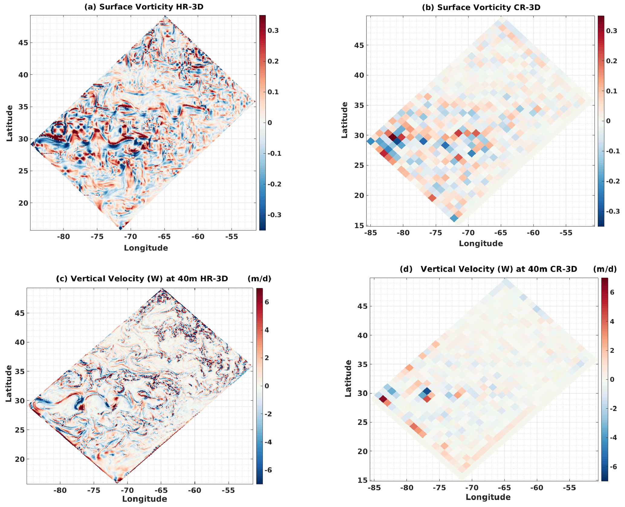
Figure 1Snapshots on 31 March of (a) surface vorticity at high resolution (HR), (b) surface vorticity at coarse resolution (CR), (c) vertical velocity at 40 m at HR, (d) and vertical velocity at 40 m at CR.
2.2 Methods
2.2.1 Simulation of trajectories
In this paper, the focus is on the analysis of ocean connectivity from Lagrangian numerical particles (Figs. 2 and 3a) deployed at different defined sites across the double-gyre current configuration, located in key areas of the circulation (Fig. 3b). For this purpose, the positions of the numerical particles at each time step (1 h) were calculated using the Lagrangian tool ARIANE (https://ariane-code.cnrs.fr/, last access: 22 May 2021). ARIANE is an open-source, offline, three-dimensional Lagrangian particle tracking model written in Fortran, and it is compatible with many ocean general circulation model (OGCM) outputs. It works by interpolating velocity values (bilinear interpolation in space and linear interpolation in time) to a given particle position using an analytical scheme (a fourth-order Runge–Kutta scheme) and advects the particle over a user-defined time step. A description of the algorithm is given by Blanke and Raynaud (1997) and Blanke et al. (2001).
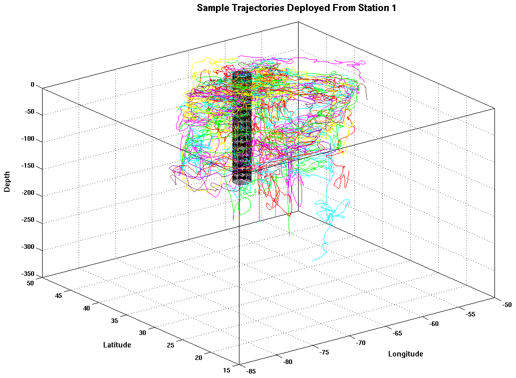
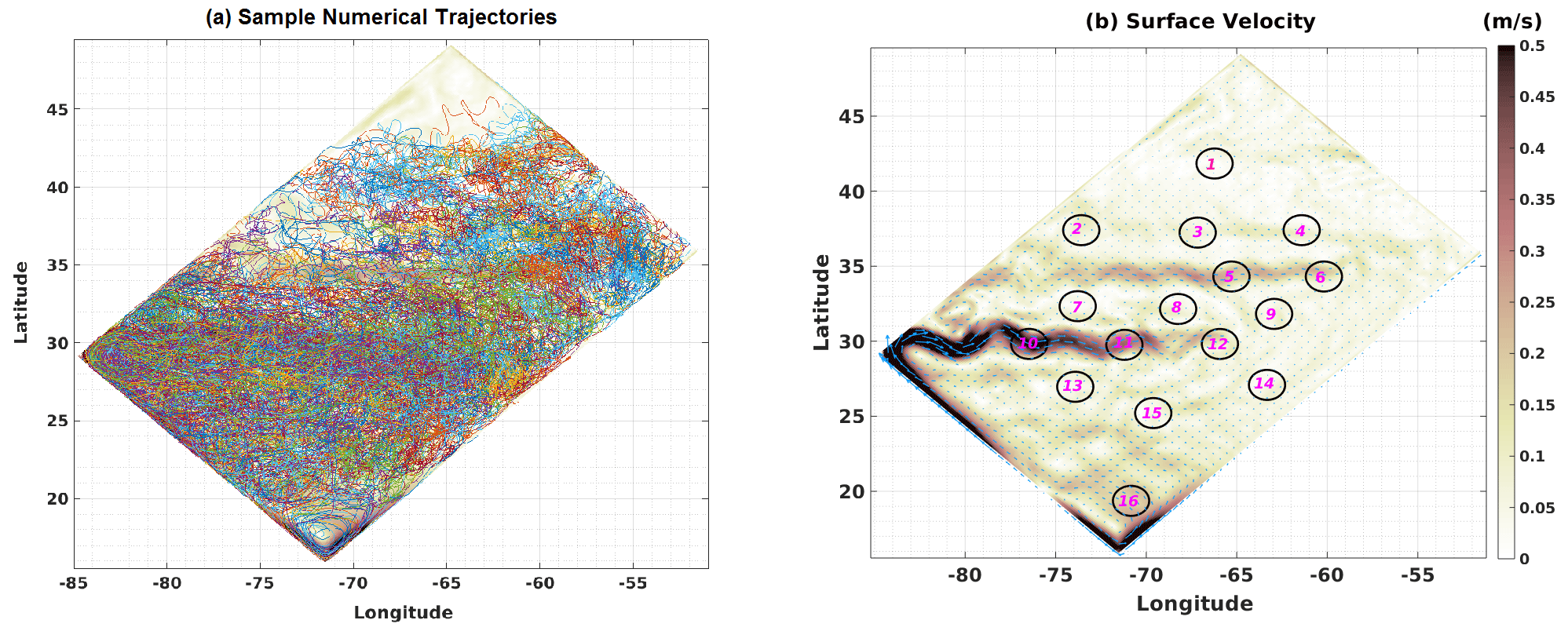
Figure 3(a) Dispersal of sample trajectories on the surface layer in HR-3D from site 13. (b) Annual mean speed and location of the sites.
Sites were defined as circular regions of 1∘ radius. This size corresponds to the grid size of the coarse-resolution velocity field. A total of 100 000 particles were deployed at each site. Such a large number of particles and the wide size of each site reduces the sensitivity of the results to the exact location of the initial position and provides statistically more robust estimates. We used 1 600 000 particles for each Lagrangian experiment. Based on the Lagrangian tool, ARIANE, particles reaching domain boundaries continue their movement along the model closed boundaries. The frequency of particle release was specified with random initial times, while the minimum duration of trajectory tracking was 1 year (the maximum integration time was 5 years). Particles were released every 1 m from the surface to the base of the mixed layer, yielding a total of 150 release locations over this depth (667 particles per meter) (Fig. 2).
We analyzed and compared the properties of three sets of Lagrangian experiments (with the same integration time), one performed using the full resolution of the velocity field in 3D (HR-3D), one performed using the filtered velocity field (CR-3D), and one using the full-resolution surface-only velocity field (HR-SL).
2.2.2 Site specification
Sites were distributed in key regions of the flow in order to examine and contrast connectivity properties between the two gyres, along the main jets, and across the jets. The exact location of the sites is arbitrary, but in order to have reliable results, we choose more than one site to represent each key region of the domain. More precisely, three sites were located along the main jet (−85 to −68∘ W and 27 to 32∘ N) on the western side of the basin (sites 10, 11, and 12, Fig. 3b), and two sites were located upstream of the secondary jet (−81 to −60∘ W and 33 to 35∘ N) at locations with lower kinetic energy (sites 5 and 6) in order to study connectivity between different parts of each jet, for example from the tails (ends) of the jets to their heads and back (see Fig. 3). In addition, other sites between the jets were selected to calculate connectivity properties between gyres (sites 1 to 4 in the subpolar gyre, sites 7 to 9 in the inter-jet region, sites 13 to 15 in the subpolar gyre). Also, five sites (1, 3, 8, 15, and 16) were aligned along the model diagonal to determine the transfer time from north to south and vice versa (Fig. 3b), but three other sites (2, 7, 13) can be used for the same purpose.
2.2.3 Lagrangian indices
Different approaches, all based on the tracking of passive Lagrangian particles, have been used to quantitatively measure connectivity between different marine sites, e.g., Lagrangian probability density functions (PDFs) (Mitarai et al., 2009; Froyland et al., 2009; Ser-Giacomi et al., 2021), transport networks (Rossi et al., 2014), and characteristic timescales (Jönsson and Watson, 2016). Some of these methods rely on the general definition of “connectivity time”, which depends on oceanographic distances and is often estimated as the mean time required for particles to move from one location to another (Cowen et al., 2007; Mitarai et al., 2009). However, in the global ocean, mean and median transit times are not well defined because each particle deployed at a given location will eventually reach all other areas of a defined domain over a sufficiently long time (Jönsson and Watson, 2016). To address this, Jönsson and Watson (2016) proposed using the “minimum connectivity time” (Min-T), defined as the fastest travel time from source to destination for numerical particles, inferred from a Dijkstra algorithm (1959). This minimum connection time shows good correspondence with genetic dispersal in marine connectivity (Alberto et al., 2011). The benefit of using the minimum connection time rather than the average transit time has been shown in previous empirical work (e.g., Mora et al., 2012; Mitarai et al., 2009; Döös, 1995; Cowen et al., 2007). Following up on these previous advances, in this study, we focus on mean and median values of minimum connectivity time for all particles traveling from one given site to another in order to obtain a clear picture of transit times. Furthermore, dispersion patterns of the numerical trajectories show the main effects of the particle release position and ocean circulation on the strength and persistence of connections between site pairs. Specifically, we will provide a comprehensive matrix containing analyses of the mean, median, and most frequent values of the minimum connection time between each selected area seeded with numerical particles.
2.2.4 Lagrangian PDF
The Lagrangian PDF approach is useful to examine the dispersion of particles by turbulent phenomena. It has been widely used in fluid mechanics (e.g., Pope, 1994; Mitarai et al., 2009; Froyland et al., 2009; Ser-Giacomi et al., 2021b). This method relies on the probability that particles have moved from one location to another during a given time interval. Since the PDF values provide an estimate of the mean dispersion properties of the numerical particles, a correct estimation of the PDF values requires a large number of trajectories (Mitarai et al., 2009); for the purpose of our study, 100 000 particles were assigned to each site. This number was set to have a significant number of particles for the connectivity estimates but was, however, limited to remain computationally manageable. The Lagrangian PDF for each site is obtained by Mitarai et al. (2009):
where ξ is the sample space related to the discretion of the Lagrangian PDF (here, a sample space of ∼ 1 km2 is applied for the calculation of the PDF fields), Sξ is the area of the sample space ξ, N is the total number of Lagrangian particles, and nξ(t) is the number of particles residing in the sample space ξ at the simulation time t.
3.1 Transit times
A quantitative assessment requires some degree of simplification due to the multiple spatial and temporal scales involved. In this framework, it is useful to determine the probability distribution of the numerical particles deployed from the different sites for different integration times (see Fig. 4 for the results obtained for site 1). After the first week of deployment, the concentration of numerical particles is larger around the starting positions, as expected. After 6 months, the particles move a short distance from their initial positions and spread over 5–10∘ of longitude, depending on the flow velocity. When particles are close to strong jets, they disperse very rapidly (2–6 months), whereas in other parts of the basin, due to slower and less energetic velocities, the dispersion occurs over a longer period (1.5–2 years).
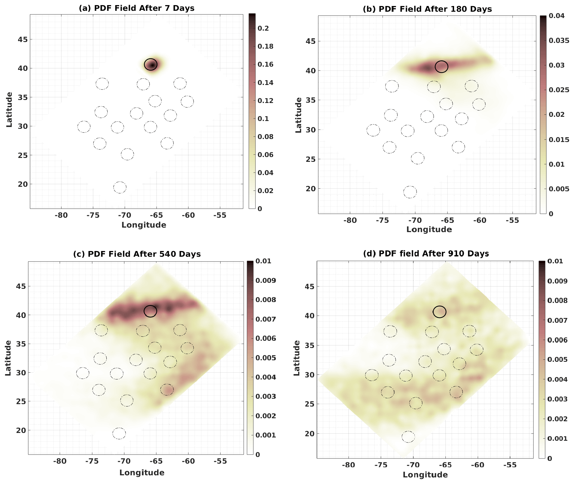
Figure 4PDF fields of the position of particles after increasing time intervals in HR-3D. After 7 d (a), after 180 d (b), after 540 d (c), and after 910 d (d).
At 1.5 years after their release, the particles deployed from the subpolar gyre (site 1) are dispersed in the entire subpolar gyre and have also penetrated the subtropical gyre along its eastern edge. Regardless of the initial deployment position, 3.5 years after deployment, almost all particles are concentrated along the two intense jets that separate the two gyres (Supplement Figs. S1–S5). For particles leaving site 1, the probability that they will reach sites 2, 3, and 4 after 2 years along the basin diagonal is between 0.2 % and 0.8 %, and for sites 5, 6, and 14, it is about 0.5 %. This means that connectivity between these sites and site 1 is achieved in less than 2 years. A uniform PDF distribution after 2.5 years for the particles from site 1 shows that in less than 900 d they have spread across more than 75 % of the basin. We also note that with longer particle lifetimes, the PDFs show similar behavior compared with the other sites (Fig. 4). After 1.5 years, particles are mostly on the eastern side of the basin, moving slowly southward due to less energetic flow in these areas (Fig. 4c, d).
In contrast, particles deployed in the main jet (Supplement Fig. S4) remain mostly close to or move slowly to the southern basin during all simulation times. This pattern reveals the strong influence of the jets on particle movement. For this case, the PDF has the highest values in the jet area and in the subtropical gyre. After 5 years, the lowest PDF values for particles reaching the jet and the subtropical gyre are associated with particles initially deployed along the western boundary of the subpolar gyre (e.g., site 2). In conclusion, the PDFs show that particles spend long periods of time in the subtropical gyre, indicating that this regional retention by highly energetic nonlinear ocean dynamics prevents rapid dispersion in all other regions. This significantly increases the mean particle transit times.
3.2 Comparison of connectivity properties between HR-3D and CR-3D
3.2.1 PDF histogram for HR-3D and CR-3D
Figure 5 shows the PDFs of the transit times of particles traveling between selected sites for HR-3D and CR-3D. The PDFs are not Gaussian and are skewed with a long tail. Figure 5a shows the PDFs of the particles deployed at site 1 in the center of the subpolar gyre and arriving at site 15 in the center of the subtropical gyre, whereas Fig. 5b shows the reverse connection, i.e., for the particles deployed at site 15 traveling to site 1. For HR-3D the first particles reach site 15 after about 200 d, and most particles reach this site after about 600 d. The latest particles continue to arrive at site 15 after 1600 d. The CR-3D PDF is shifted in time with respect to HR-3D, with particles only reaching site 15 after about 300 d. The width of the CR-3D PDF is broader than that of the HR-3D, suggesting a larger but slower spread of particles across the domain before reaching site 15. The median transit time from site 1 to site 15 is 751 d, while the minimum transit time in this direction is 201 d. The Lagrangian connections for particles deployed at site 15 and reaching site 1 (i.e., connectivity in the opposite direction as for the previous case) show a longer transit time and a greater spread for both simulations (Fig. 5b). The CR-3D PDF shows an even larger delay in arrival time compared to HR-3D.
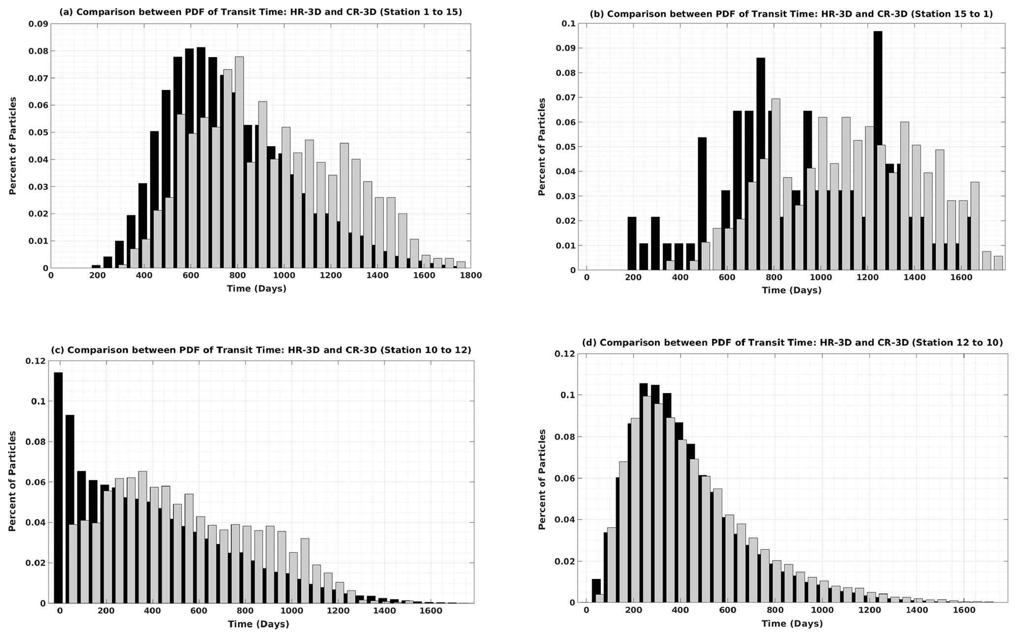
Figure 5Comparison of HR-3D (black) and CR-3D (gray) transit time distributions (a) for particles initially deployed from site 1 to site 15, (b) from site 15 to site 1, (c) from site 10 to site 12, and (d) from site 12 to site 10.
For HR-3D, the mean time required for particles to travel along the basin diagonal from the subpolar gyre to the subtropical gyre (i.e., from site 1 to site 15) is about 796 d, and the modal time is 559 d compared to 989 and 1262 d, respectively, for the reverse connection (i.e., from south to north, site 15 to site 1). This means that the northward movement along the diagonal is faster than the southward movement. The PDF distributions cover almost the same time range, although the general shape is different. The same transit times (mean and most frequent values) for CR-3D are 891 and 644 from north to south and 1162 d and 1315 from south to north. The minimum time required for particles from south to north (site 15 to site 1) in the HR model is 153 d shorter than in the CR model (201 vs. 355 d).
To compare the Lagrangian connectivity between the most distant sites with the sites closer to each other and within the main jet ([30∘ N, −85∘ W], [30∘ N, −70∘ W], where the mean energy and eddy kinetic energy show the highest values) we computed the transit time statistics between sites 10 and 12. The results are shown in Fig. 5c for the direct connection (site 10 to site 12) and in Fig. 5d for the opposite direction (site 12 to site 10). They suggest that the connection along the eastward jet is faster (as expected): the first particles and largest number of particles arrive within 10 d in HR-3D, whereas for CR-3D the arrival time of the first particles is longer (40 d) and the PDF distribution is larger.
As foreseen, the intense and highly energetic eastward jet moves the particles very rapidly eastward, although fine-scale circulation (mesoscale eddies and filaments) generated at the edges of the jet disperses the particles that reach site 12 almost continuously (albeit in decreasing numbers) until about 1400 d. The minimum and median transit times for the HR-3D simulation are 11 and 348 d, while these values are larger for CR-3D (64 and 213 d, respectively). The CR-3D velocity field induces slower connections because the peak velocity of the jet is lower and its width larger. The connection time in the coarser velocity field is relatively continuous until about 1300 d. This can be explained by the particles traveling through the larger-scale recirculation cells of the subpolar and subtropical gyres before reaching site 12.
In contrast, the HR-3D and CR-3D PDFs have a more similar shape and distribution for the opposite (westward) connection, with the first particles reaching site 10 from site 12 in less than 50 and 452 d on average and 546 d in median time (Fig. 5d). The minimum and mean transit times for particles from site 12 to site 10 are longer. The modal value is 260 d, and the median transit time is 398 d. The similarity in connectivity behavior for the opposite (westward) connection for both velocity fields suggests that the particles move through the mean larger-scale recirculation cells and follow the common pathways.
The above PDF results for both simulations (HR-3D and CR-3D) clearly show the impact of the ocean fine-scale dynamics, which increase the efficiency of the current advection and accelerate the particle motion; in this case, for the CR-3D simulation, the PDFs of transit times are wider with longer mean and minimum transit times due to insufficiently resolved turbulent motions.
3.2.2 Minimum and median transit time as a function of geographical distance
Figure 6 shows the minimum and median values of transit time as a function of distance computed in HR-3D for sites along the basin diagonal. The results indicate that with increasing distances, the transit times (minimum and median) increase linearly. For the particles initially deployed from site 1, the results show almost the same behavior for median and minimum time, except for connections between site 1 and sites 12 and 15. The shortest minimum transit time in a diagonal direction is from site 8 to site 12 with a value of 2 d. The fastest connection based on median transit times is from site 8 to site 5, with a value of about 95 d. The minimum transit times from south to north and north to south are almost identical (about 200 d). The longest minimum transit time is for the particles moving from site 12 to site 1 at 240 d, with a median value of 1109 d. This suggests that the intense fine-scale circulation facilitates connections between site 8 (which is located in the middle of the diagonal transect) and site 12 (at the eastern end of the main jet) and slows those between sites 8 and 5 (a median transit time of 225 d versus 95 d). In general, the Lagrangian transit times (median and minimum) for a site pair located at the same distance along the basin diagonals differ. Such a difference arises from the complex trajectories, followed by the numerical particles, and is induced by the small-scale simulated dynamics. On the other hand, for site pairs located at a shorter distance (less than 6∘), the minimum transit time is less than 55 d regardless of the site location.
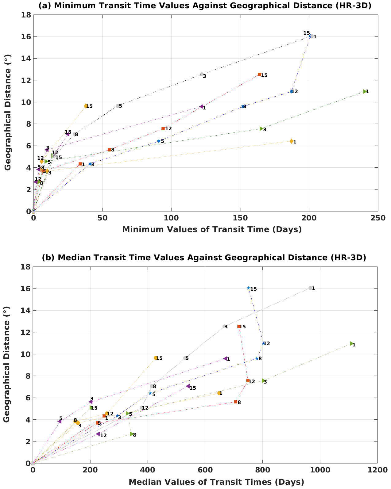
Figure 6HR-3D minimum (a) and median (b) transit time against geographical distance. Blue: particles initially deployed from site 1; red: particles initially deployed from site 3; yellow: particles initially deployed from site 5; purple: particles initially deployed from site 8; green: particles initially deployed from site 12; gray: particles initially deployed from site 15.
To more quantitatively assess the differences in connectivity between HR-3D and CR-3D, Fig. 7 shows the comparison of minimum and median transit times computed for a subset of sites for the two Lagrangian simulations. The results clearly indicate that the minimum and median transit times in HR-3D are significantly lower than for the coarse-resolution configuration. In HR-3D, the resolved nonlinear dynamics induce intense currents, and the particles move much faster than in CR-3D, in particular for the sites located along the two main jets. Figure 7 suggests that for distant sites, CR-3D will not provide realistic information about the connection time between sites. The lack of fine-scale motions in the coarse-resolution simulation leads to significant delays in the advection of numerical particles, especially in areas where mesoscale variability plays an important role in particle displacement. The results obtained for particles deployed from site 15, for short-range connections (distances less than 10∘), show a better match for the median transit time for both configurations: HR-3D and CR-3D. Based on a minimum connection time of less than 50 d, there is some convergence between HR-3D and CR-3D for particles deployed from site 1, whereas large differences arise for distances greater than 6∘ and for areas that include hotspots of high eddy kinetic energy. In addition, in HR-3D, the particles disperse not only faster but also more uniformly than in CR-3D, which reduces transit times between sites. From south to north along the diagonal, the results of both simulations (median values of transit times) are similar, showing that in this direction particles follow pathways less affected by small-scale ocean instabilities.
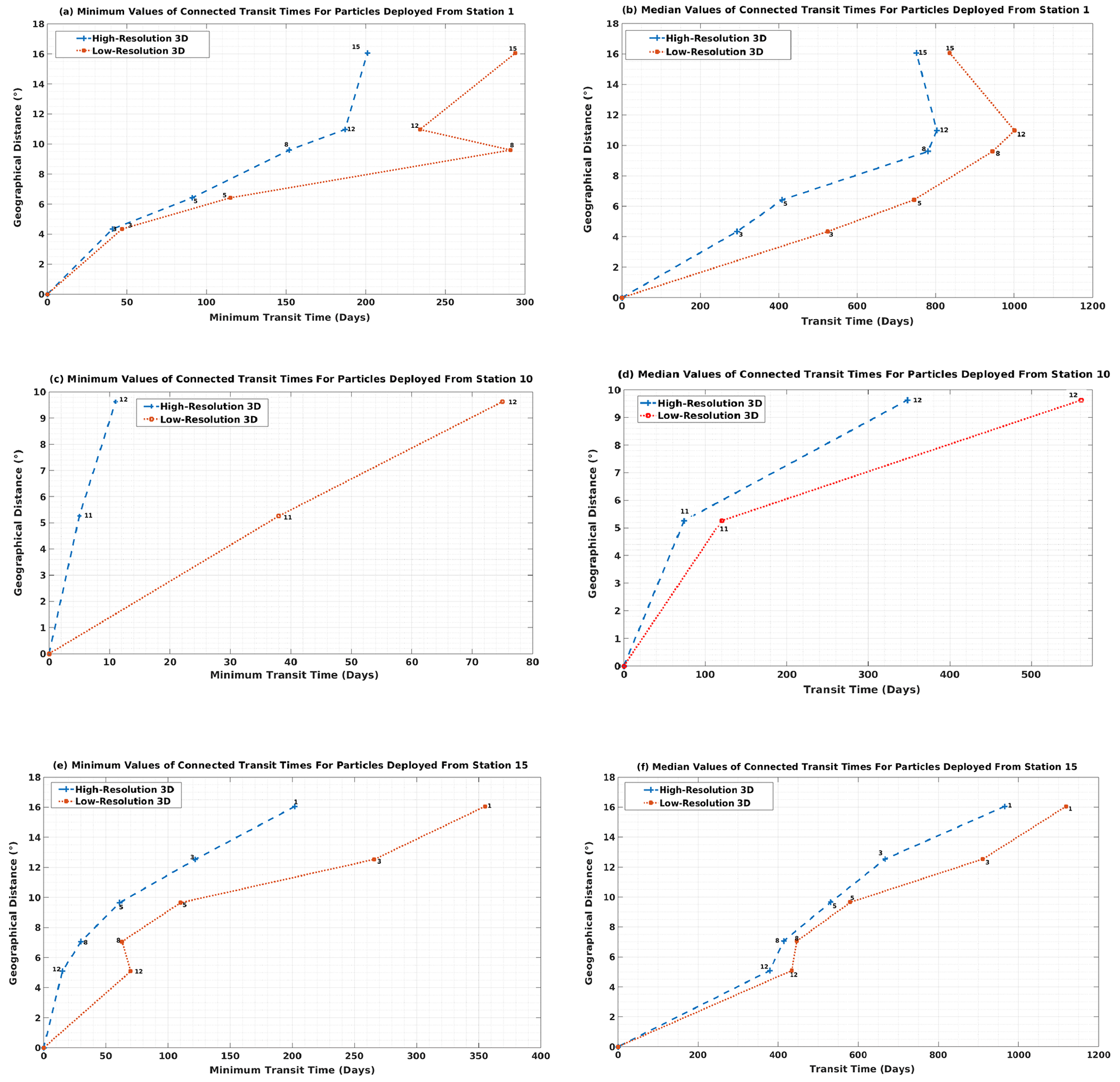
Figure 7Comparison of HR-3D and CR-3D minimum and median transit times. (a, b) Along the diagonal direction for particles initially deployed from site 1. (c, d) Along the front for particles initially deployed from site 10. (e, f) Along the diagonal direction for particles initially deployed from site 15.
3.2.3 Examples of depth arrival PDF for HR-3D and CR-3D
Connectivity studies of marine ecosystems commonly integrate Lagrangian trajectories using 2D surface velocity fields because the focus is on passively drifting biological species (e.g., plankton, fish larvae, algae). We test the robustness of such a strong assumption by integrating Lagrangian particles in a 3D framework: for each site at the initial integration time step, particles are distributed over the water column extending from the surface to the base of the mixed layer (which can be as deep as 150 m). Then, the particles are advected by the 3D flow, without any depth constraint. In this way, we can test whether particles in the upper ocean remain at the same depth throughout their journey and thus confirm or invalidate the soundness of using 2D and not 3D velocity fields for marine ecosystem connectivity estimates.
Figure 8a and b show the PDFs of the mean arrival depth of particles initially deployed from site 1 and arriving at site 15 (left panel), as well as in the opposite direction from site 15 to site 1 (right panel). Our analysis indicates that the majority of particles in both simulations remain in the depth range below 165 m without moving much deeper, although the peak is deeper in the south-to-north motion for HR-3D and CR-3D and is quite noisy.
The HR-3D and CR-3D PDFs (Fig. 8a, b) indicate that the particles are almost twice as deep in the south–north connection as in the north–south connection. From south to north, a small percentage of the particles reach the bottom layer (more than 450 m deep) where frictional processes alter the dynamics and thus play an important role in the transit of the numerical particles. These processes do not appear to play a role in the north–south movement.
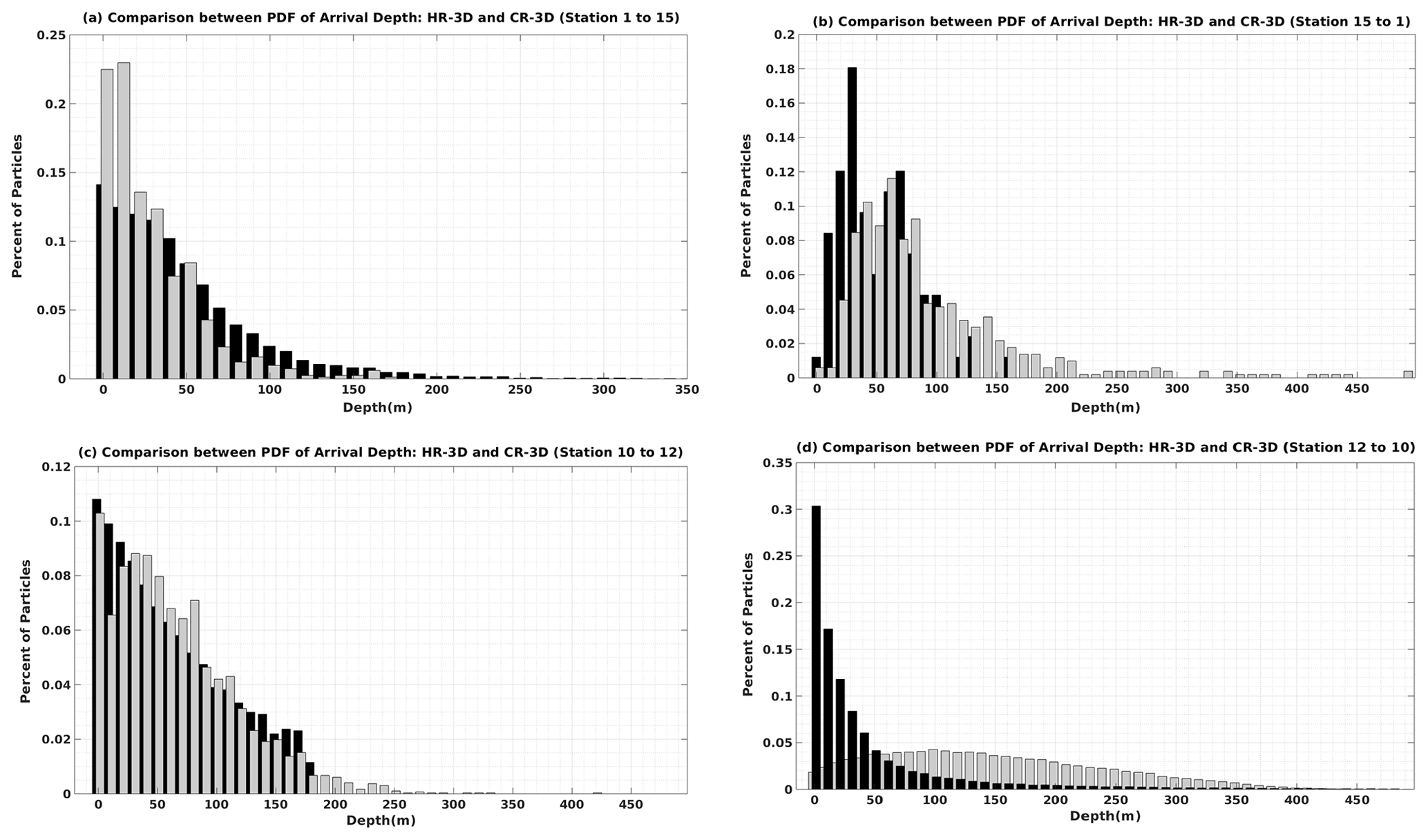
Figure 8Comparison of HR-3D (black) and CR-3D (gray) arrival depth distributions (a) for particles initially deployed from site 1 to site 15, (b) from site 15 to site 1, (c) from site 10 to site 12, and (d) from site 12 to site 10.
The PDF of the mean arrival depth of particles deployed from site 10 to site 12 (Fig. 8c) shows that for the trajectories simulated by the high-resolution fields there is a tail that extends down to 175 m, with a slightly higher percentage of particles in the subsurface layer compared to the CR results, and the particles in the upper layer tend to travel faster than those are at greater depths, as velocities decrease with depth.
On the other hand, although the mean PDF of arrival depth for particles moving from site 10 to site 12 shows the same behavior in the HR and CR 3D velocity fields, in the opposite direction (site 12 to site 10) the PDF distributions for the two simulations are completely different, considering that the distribution is overall flatter in CR-3D than in HR-3D with a long tail extending to 380 m in depth.
A comparison of the mean arrival depth of the numerical particles deployed from site 12 to site 10 (Fig. 8d) in the HR case shows that the majority of the particles remain within 50 m of the surface layer, while in the opposite direction, some particles move to greater depths up to 150 m. Furthermore and as already mentioned, the numerical trajectories simulated in CR are relatively uniform across the upper layer where they were initially seeded. Indeed, in CR, more than 70 % of the particles deployed from site 12 and arriving at site 10 remain close to the surface mixed layer and the subsurface, where the effects of turbulence at different scales on the numerical particle distribution are more detectable.
Mainly, for all cases examined, in HR-3D, the particles tend to remain in the subsurface layer due to the larger effects of coherent vortices as well as other structures such as filaments and eddies. The PDFs of arrival depth indicate that the differences between HR-3D and CR-3D are not limited to the arrival time, but are also detectable on different 3D pathways for each case, resulting in significant changes in the arrival depth. Thus, we can add that the depth results differ depending on the direction of motion. Also, the peak for all HR-3D cases is at the depth of less than 10 m except for the south–north motion, which shows that in this direction, the particles move more in the vertical direction due to weaker stratification at depth and less turbulence in the surface layer.
3.2.4 Mean connection time fields for sample sites
The mean connection times from three sites (north, west, and south of the basin) are shown in Fig. 9. Figure 9a shows that the particles from site 1 follow pathways that require the longest time to connect to sites in the subtropical gyre and western boundary current regions, such as sites 10, 11, 12, 13, 15, and 16. The particles reached a depth of 150 m from the surface layer near the eastern side of the basin between (−60 to −55∘ W) and (37.5 to 42.5∘ N) near site 4, although the transit time from site 1 to site 4 was less than 300 d (not shown). Particles deployed from site 1, moving from south to north, take almost 500 d, while they take about 400 d to travel the same distance from north to south. The shortest mean transit times are between sites 1 and 4 and between sites 1 and 3 (both less than 350 d), while the longest connections (from site 1) are associated with sites 10 and 11 (944 and 915 d, respectively). This was expected since these sites are located along the strong jet. Note that the mean arrival depth for the shortest transit time is about 35 m (not shown), while for the longest transit time, the mean arrival depth is over 100 m below the surface layer. For site 1, the mean transit time is 1.25 times greater in CR-3D than in HR-3D. Figure 9a and d show similar distributions, although the connection times between site 1 and sites at 30–40∘ latitude and −72.5 to −62.5∘ longitude differ significantly.
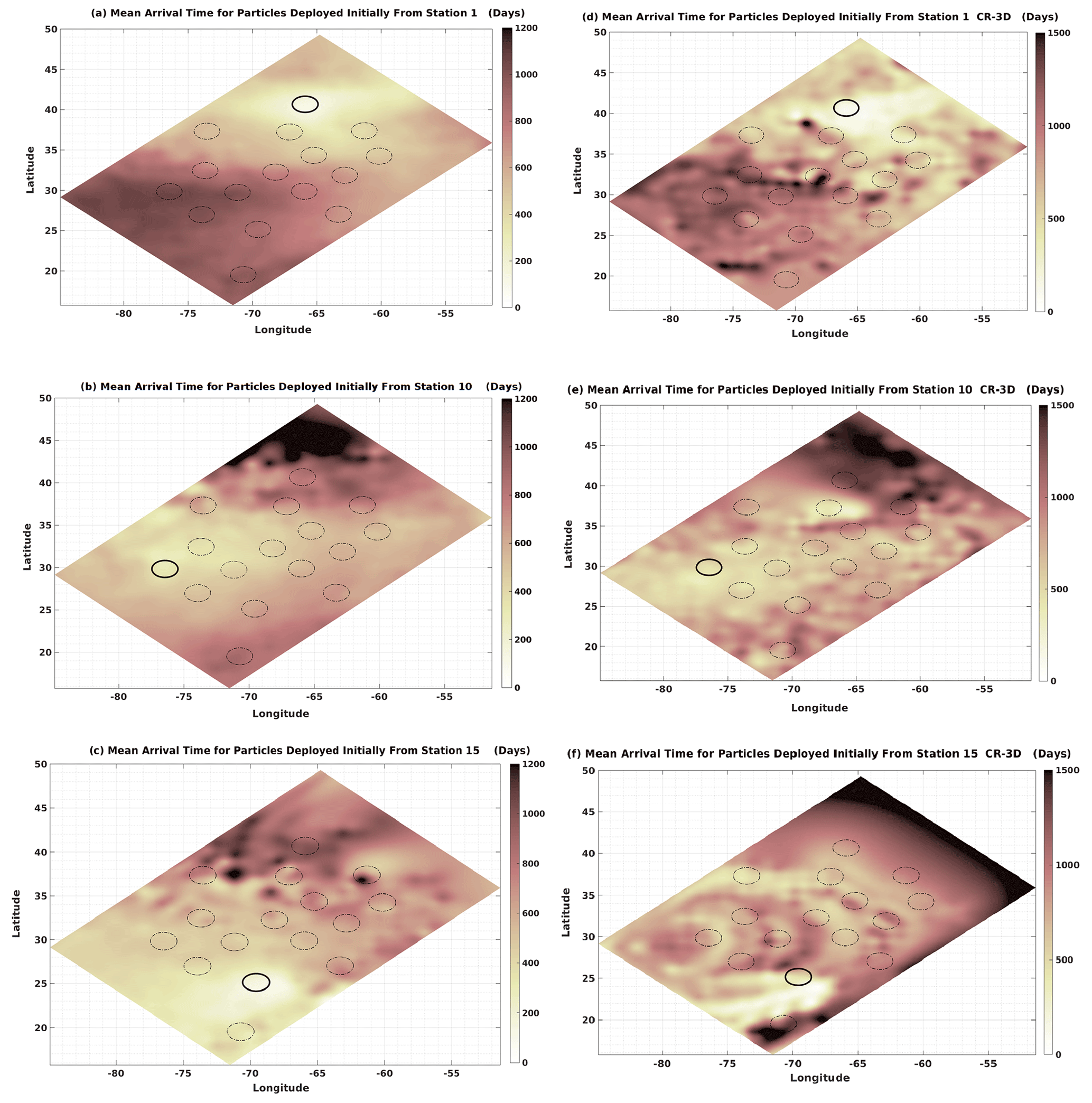
Figure 9Comparison of HR-3D and CR-3D mean arrival (transit) time (a, d) for particles initially deployed from site 1, (b, e) from site 10, and (c, f) from site 15.
Figure 9b shows the mean arrival time from site 10. As shown in the mean transit time map, a large area connecting the southwestern region to the northeastern region has the lowest values. This clearly shows the direct connection of the particles seeded in the main jet, which travel fast and reach these areas rapidly. For these regions, the mean arrival depth values were less than 70 m (not presented here). The longest connection times are associated with sites 1 and 16 for particles that initially started from site 10. These particles took over 1200 d to arrive north of site 1 and appear to be in a shadow dynamical region that is not directly connected to the jet. The results are similar in CR-3D for site 10, although the transit time is significantly higher in the coarser simulation than in the finer-resolution simulation (Fig. 9b, e).
Figure 9c and f show the mean transit time of particles initially deployed from site 15 to other sites for HR-3D and CR-3D. The distribution is remarkably different. In the CR-3D simulation, the connection is fast in the southernmost region and does not allow some transit times to be modeled acceptably, such as the motion from site 15 to the areas around site 16 and from site 15 to the northern part of the basin (north of site 1). This figure clearly indicates that the particles in CR-3D move in a less dynamical velocity field, especially for trajectories moving from south to north and from south to west. The shortest connection time from site 15 and site 14 in HR-3D is less than 13 d, while it is 50 d for CR-3D.
In all simulated cases, we were able to differentiate the impacts of highly energetic small scales on particle transit times between different sites. As shown in the surface vorticity snapshots in Fig. 1, filamentary structures and small eddies in the jets separating the two gyres and the subpolar region act as transport barriers, for example for particles traveling from site 15 to site 1.
3.3 Transit time matrices between site pairs
3.3.1 Comparison of transit time between site pairs for HR-3D and CR-3D
To complete the study, we compared the minimum and median transit times for all defined sites in the basin. We evaluate the sensitivity of the transit time matrix to the currents provided by two different cases: HR-3D and CR-3D. Specifically, in this section, we provide a complete matrix containing the analyses of the median and minimum connection time between each selected area seeded with numerical particles.
Figure 10 provides an overview of the structure and time characteristics of the connectivity between sites. It shows that the connectivity between the northern and southern sites is the weakest (the connection is the longest in terms of both the minimum and median times) and it is not symmetric. The longest connection is between the northern and southern sites. The fastest connection is along the main jet (site 10 to site 13). This matrix also highlights the difference in the definition of connectivity when applying the minimum or the median time. The latter is 3 to 4 times larger than the first. Moreover, the minimum time for CR is slightly larger than for HR and varies between 10 d and 4 months. The difference increases notably for the median time, including along the principal jet (with a delay in arrival time ranging from 1 to 6 months).
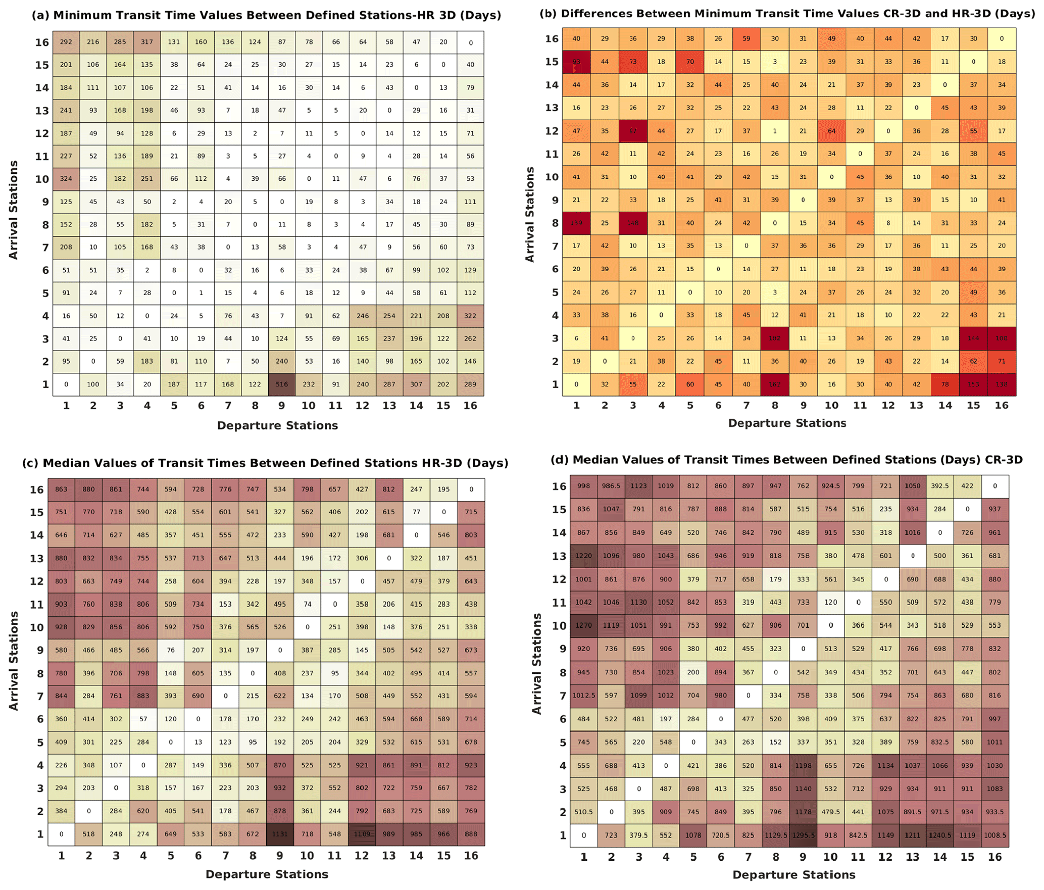
Figure 10Comparison of HR-3D and CR-3D minimum and median transit times between site pairs, (a) minimum transit time for HR-3D, (b) difference between minimum transit time for CR-3D and HR-3D (CR3D − HR3D), (c) median transit time for HR-3D, and (d) median transit time for CR-3D.
The longest connection is for particles moving from the northern edge of the subpolar gyre (site 1) to the easternmost region between the two zonal jets separating the gyres (site 9), with minimum and median transit times of 516 and 1131 d, respectively, for HR. For CR and for the same sites, these times increase by an additional 30 and 164.5 d, respectively. On the other hand, the shortest connection is between sites 6 and 5, along the northern zonal jet, where we obtained 1 and 13 d as minimum and median transit times, respectively, for HR. Note that this result is related to an increased efficiency of the particle advection due to the resolved small-scale nonlinearities, which seem to be particularly active in this part of the basin. The resolved small scales act as stirring structures that accelerate the movement of particles around, for example, the peripheries of mesoscale eddies and along filaments. In addition, areas with longer transit times show larger differences between HR and CR (for example, departures from sites 14, 15, and 16 and arrivals at sites 1, 2, and 3).
3.3.2 Comparison of transit time matrices for HR-3D and HR-SL
To determine whether the Lagrangian properties of oceanic flows can be evaluated in 2D (limited to the surface layer of the ocean), rather than by including the full 3D framework, we compare connectivity properties between defined sites for 2D and 3D high-resolution simulations (Fig. 11 and Supplement Fig. S6). The results show that the transit times for numerical particles deployed in the surface layer are generally shorter than those for particles that started in deeper layers (3D), although there are some exceptions such as the motion from site 2 to sites 6 and 7: in this direction, a high percentage of particles in the surface layer need a longer transit time to reach the final destination than similar particles in deeper layers. This is due to vertical fluxes associated with the displacement of isopycnals by internal dynamics (e.g., eddy pumping or eddy–eddy interaction). Therefore, areas with similar values of connectivity properties in the 2D and 3D simulations suggest that vertical motions for these regions are not strong enough to add complexity to trajectories.
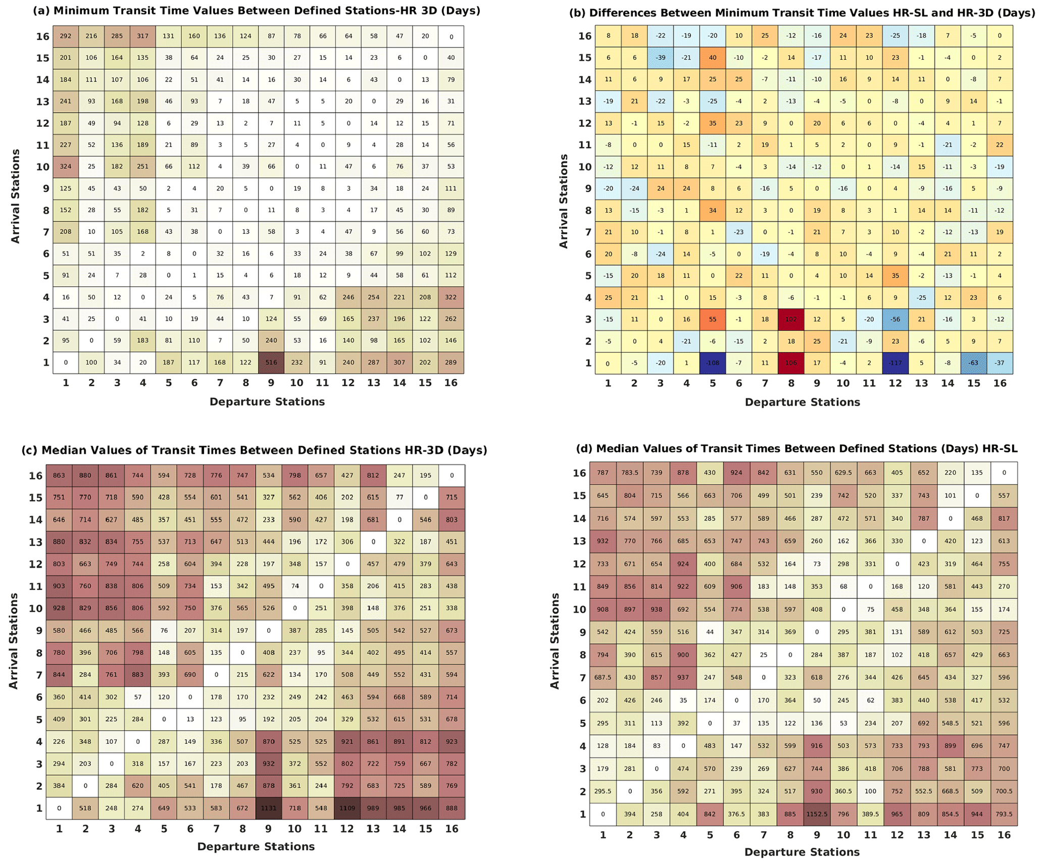
Figure 11Comparison of HR-3D and HR-SL minimum and median transit times between site pairs, (a) minimum transit time for HR-3D, (b) difference between minimum transit time for HR-SL and HR-3D (HRSL − HR3D), (c) median transit time for HR-3D, and (d) median transit time for HR-SL.
Although there are many similarities between the median transit time matrices for the HR-3D and HR-SL cases (Fig. 11), the distribution of the minimum transit time values shows differences; the main reason is related to vertical movements. In other words, the vertical dimension of the trajectories that exists in HR-3D gives the possibility to establish more pathways between the different areas. This result provides important insight into connectivity properties in the ocean: while 2D simulations provide useful information on transit times, it is necessary to understand the rate of connections using 3D simulations.
In conclusion, both 2D ocean connectivity and 3D ocean connectivity are important tools for understanding the movement of water and other properties within the ocean, but 3D connectivity provides a more complete picture by taking into account the full three-dimensional movement of water and thus life.
Lagrangian connectivity analysis utilizes sets of numerical particle trajectories to identify connecting pathways, as well as timescales and transport between oceanic regions. This is a powerful tool to coherently study the connection between different areas in the ocean. The current study is one of the first large-scale studies to use high-resolution ocean flow data and particle tracking to describe connectivity patterns in a large-scale (although idealized) basin.
In this paper, the focus was on analyzing the connectivity of different sites in a double-gyre ocean model using a Lagrangian approach with numerical particles. A total of 16 sites were specified and at each site 100 000 particles were used for the numerical analysis. Lagrangian properties such as mean, median, and modal transit times were calculated to examine connectivity properties in the North Atlantic. In addition, the probability density functions (PDFs) of transit times and mean arrival depths for different simulations were compared. The analysis used high-resolution 3D velocity fields (HR-3D), HR surface velocity (HR-SL), or velocity fields averaged over a coarser-resolution grid (CR-3D).
The Lagrangian PDF modeling approach was implemented for the sample sites in all the simulations. The particles have different trajectories to reach their final destinations due to the small-scale motions induced by the resolution of the fine-scale dynamics. The results indicate that particles that remain in the surface layer or near the subsurface layer move faster due to intensified velocities resulting from simulating the fine-scale circulation. In the deeper parts of the basin, particles need more time to reach their final site, as at depth, the velocity intensity decreases due to the effect of the nonlinear dynamics. This finding is confirmed by comparing the PDF of the 2D surface layer simulation with other simulations.
Fine-scale movements, especially in the upper 50 m of the surface layer, play an important role in particle motion. The numerical particles in the two simulations (HR-3D and CR-3D) show significantly different PDF distributions, especially for movement from the western part of the basin to the eastern part (e.g., from site 10 to sites 4 and 2, see Supplement Fig. S7). It was also found that the particles transported by the high-resolution velocity fields tend to move to deeper parts of the basin compared to the CR-3D simulation.
In the 5-year simulation based on HR-3D velocity fields, the longest route was obtained for particles deployed from site 9 (in the eastern part of the western boundary current extension) to site 1 (in the subpolar gyre), with an average transit time of 1145 d. This is due to less energetic flow in the areas close to these sites. In contrast, transit times along the principal zonal jet (site 10 to site 11) represent the shortest and fastest routes, with an average transit time of 179 d.
As expected, the numerical particles remain concentrated around their starting position during the first week after their deployment. But 3 years after their departure and independently of their initial deployment positions, almost all particles were concentrated along the two zonal jets. These jets act as attraction hubs that eventually capture most of the particles. Based on the mean arrival depth at the sample sites, we can see that the particles move toward deeper depths in the interior of the ocean due to the strong nonlinear velocity fields that develop around these jets on the western side of the basin, with a direct impact on the vertical motion of the numerical particles.
Our results emphasize the fact that because ocean circulation is turbulent at horizontal scales of 10–100 km, it is not relevant to assess connectivity properties using climatologies or low-resolution (> 100 km) velocity fields; moreover we show that connectivity in the ocean is not 2D but 3D and that assessments based on 2D fields may significatively alter the results.
Lagrangian trajectories simulated with the coarse-resolution velocity fields do not sufficiently show the effect of mesoscale eddies on particle dispersion, which results in unreliable Lagrangian indices (e.g., transit time) compared to estimates based on HR model simulations. The CR ocean flow simulation used in this study, with a spatial resolution of ∼ 100 km, is inadequate to describe the mesoscale circulation. Yet, this fine-scale variability has been shown to significantly shape and change the connectivity of the North Atlantic.
In this context, our results show that the use of high-resolution velocity fields, as opposed to coarse-resolution fields, resulted in a reduction of 39 % in mean transit time (we divided the difference between the transit time, i.e., “transit timeHR3D − transit timeCR3D” or “transit timeHR3D − transit timeHR2D” by the transit timeHR3D). This suggests that the use of high-resolution velocity fields allows for a more accurate representation of the complex flow dynamics in the region and results in faster particle transport. The CR is less smooth than the HR due to the dispersion process. In the HR case, the simulated ocean dynamics disperse the particles more than in the CR case, and the numerical particle concentration in the HR case is smoother. In the HR case, the flow field is more turbulent and contains more small-scale dynamical structures than in the CR case. These small-scale features can trap and release particles in batches or form blocking patterns, resulting in high particle concentrations in some regions. However, due to the chaotic nature of the flow field, these concentrations are not maintained and the particles are eventually dispersed throughout the domain, resulting in a smoother concentration distribution. In contrast, the CR simulation has a smoother and more predictable flow field, resulting in a more uniform dispersion of particles and a less fluctuating concentration distribution. This may result in a less smooth concentration distribution than in the HR simulation.
Moreover, the study also found that taking into account the full three-dimensional (3D) velocity instead of just surface fields resulted in an increase of 8.4 % in the mean transit time. This suggests that the vertical component of the velocity field significantly affects the transport behavior of the particles and that accounting for this vertical component leads to a more accurate representation of their transport patterns. Overall, these findings highlight the importance of considering the resolution and dimensionality of the velocity fields when studying the transport behavior of particles in the study region.
In particular, in coarse-resolution simulations, the dispersion of particles is degraded. This results in longer transit times. It also limits the connection between water particles at different depths. A possible solution to overcome this problem when integrating Lagrangian trajectories using the velocity calculated in coarse-resolution simulations is to parameterize the missing dispersion. Some methods have been proposed in the literature. The simplest parameterization consists of adding a random walk to the successive position of each particle, which is compatible with an advection–diffusion equation and is equivalent to a stochastic “Markovian” parameterization (Berloff and McWilliams, 2002). However, this stochastic parameterization does not adequately reproduce the small-scale ocean dynamics that involve consistency in advection (Klocker et al., 2012a, b; Veneziani et al., 2004). Different Markov parameterizations of higher order have been proposed in an attempt to better reproduce the effect of the small-scale ocean dynamics (Berloff and McWilliams, 2002; Griffa, 1996; Rodean, 1996; Sawford, 1991). Other improved parameterizations include particle looping due to eddy coherence (Reynolds, 2002; Veneziani et al., 2004), as well as relative dispersion between different particles (Piterbarg, 2002). While these methods have been developed and applied to horizontal flows, recent developments include an isopycnal Markov-0 (Spivakovskaya et al., 2007) or shear-dependent formulation (Le Sommer, 2011) and, more recently, an isoneutral Markov-1 formulation (Reijnders et al., 2022). The latter appears to better mimic the coherent behavior of the 3D ocean dispersion at small scales. It would be interesting in future work to evaluate how such methods, applied in a Lagrangian framework, might improve the results we obtained with a coarse-resolution field.
In conclusion, the present study highlights the importance of small-scale variability in determining patterns of connectivity and provides detailed information on Lagrangian connectivity in the North Atlantic. Our results can guide the spatial scales at which future OGCMs should be run for reliable connectivity analysis; moreover, for Lagrangian studies, we advocate refining OGCMs to the appropriate resolution with sufficient spatiotemporal accuracy.
Major parts of the data and analytical codes utilized in this study can be accessed through the following link: https://doi.org/10.5281/zenodo.8123776 (Hariri, 2023). Should any inquiries or requests for additional details arise, please reach out to the corresponding author at saeed.hariri@io-warnemuende.de. We actively promote the utilization and dissemination of our data and code to foster further research and scientific progress.
The supplement related to this article is available online at: https://doi.org/10.5194/os-19-1183-2023-supplement.
SH and SSP contributed to the data analysis and preparing the figures. SH, SSP, BBL, and ML contributed to the paper writing and design of the Lagrangian experiments. All authors reviewed and accepted the final version of the paper.
Publisher's note: Copernicus Publications remains neutral with regard to jurisdictional claims in published maps and institutional affiliations.
The authors would like to express their great appreciation to Daniele Iudicone and Laurent Bopp for their insightful discussions. The authors also thank three anonymous reviewers for helpful comments that improved earlier versions of this study. We also acknowledge the mesoscale calculation server CICLAD (http://ciclad-web.ipsl.jussieu.fr, last access: 15 August 2021) dedicated to the Institute Pierre Simon Laplace modeling effort for technical and computational support.
This research has been supported by the Agence Nationale de la Recherche (grant no. ANR-11-BTBR-0008).
The publication of this article was funded by the Open Access Fund of the Leibniz Association.
This paper was edited by Ismael Hernández-Carrasco and reviewed by three anonymous referees.
Alberto, F., Raimondi, P. T., Reed, D. C., Watson, J. R., Siegel, D. A., Mitarai, S., Coelho, N., and Serrão, E. A.: Isolation by oceanographic distance explains genetic structure for Macrocystis pyrifera in the Santa Barbara Channel, Mol Ecol., 20, 2543–2554, https://doi.org/10.1111/j.1365-294X.2011.05117.x, 2011.
Berloff, P. S. and McWilliams, J. C.: Material transport in oceanic Gyres, Part II: Hierarchy of stochastic models, J. Phys. Oceanogr., 32, 797–830, https://doi.org/10.1175/1520-0485(2002)032<0797:mtiogp>2.0.co;2, 2002.
Bharti, D. K., Katell Guizien, M. T., and Aswathi-Das, P. N.: Vinayachandran, Kartik Shanker, Connectivity networks and delineation of disconnected coastal provinces along the Indian coastline using large-scale Lagrangian transport simulations, Limnology and Oceanography, Assoc. Sci. Limnol. Oceanogr., 67, 1416–1428, https://doi.org/10.1002/lno.12092, 2022.
Blanke, B. and S. Raynaud.: Kinematics of the Pacific Equatorial Undercurrent: An Eulerian and Lagrangian approach from GCM results, J. Phys. Oceanogr., 27, 1038–1053, https://doi.org/10.1175/1520-0485(1997)027<1038:KOTPEU>2.0.CO;2, 1997.
Blanke, B., Speich, S., Madec, G., and Döös, K.: A global diagnostic of interocean mass transfers, J. Phys. Oceanogr., 31, 1623–1642, https://doi.org/10.1175/1520-0485(2001)031<1623:AGDOIM>2.0.CO;2, 2001.
Blanke, B., Bonhommeau, S., Grima, N., and Drillet, Y.: Sensitivity of advective transfer times across the North Atlantic Ocean to the temporal and spatial resolution of model velocity data: Implication for European eel larval transport, Dynam. Atmos. Ocean., 55/56, 22–44, https://doi.org/10.1016/j.dynatmoce.2012.04.003, 2012.
Cotroneo, Y., Celentano, P., Aulicino, G., Perilli, A., Olita, A., Falco, P., Sorgente, R., Ribotti, A., Budillon, G., Fusco, G., and Pessini, F.: Connectivity Analysis Applied to Mesoscale Eddies in the Western Mediterranean Basin, Remote Sens., 13, 4228, https://doi.org/10.3390/rs13214228, 2021.
Cowen, R. K., Gawarkiewicz, G., Pineda, J., Thorrold, S., and Werner, F. E.: Population connectivity in marine systems An Overview, Oceanography, 20, 14–21, 2007.
Dever, E. P., Hendershott, M. C., and Winant, C. D.: Statistical aspects of surface drifter observations of circulation in the Santa Barbara Channel, J. Geophys. Res.-Ocean., 103, 24781–24797, https://doi.org/10.1029/98JC02403, 1998.
Dijkstra, E. W.: A note on two problems in connexion with graphs, Numer. Math., 1, 269–271, https://doi.org/10.1007/BF01386390, 1959.
Döös, K.: Interocean exchange of water masses, J. Geophys. Res.-Ocean., 100, 13499–13514, https://doi.org/10.1029/95JC00337, 1995.
Drouet, K., Jauzein, C., Herviot-Heath, D., Hariri, S., Laza-Martinez, A., Lecadet, C., Seoane, S., Sourisseau, M., Plus, M., Lemée, R., and Siano, R.: Current distribution and potential expansion of the harmful benthic dinoflagellate Ostreopsis cf. siamensis towards the warming waters of the Bay of Biscay, North-East Atlantic, Environ. Microbiol., 23, 4956–4979, https://doi.org/10.1111/1462-2920.15406, 2021.
Fischer, H. B., List, J. E., Koh, R. C., Imberger, J., and Brooks, N. H.: Mixing in Inland and Coastal Waters, Academic Press, New York, https://doi.org/10.1016/C2009-0-22051-4, 1979.
Froyland, G. and Padberg, K.: Almost-invariant sets and invariant manifolds Connecting probabilistic and geometric descriptions of coherent structures in flows, Physica D, 238, 1507–1523, https://doi.org/10.1016/j.physd.2009.03.002, 2009.
Froyland, G., Stuart, R. M., and van Sebille, E.: How well-connected is the surface of the global ocean?, Chaos, 24, 033126, https://doi.org/10.1063/1.4892530, 2014.
Gaylord, B. and Gaines, S. D.: Temperature or transport? Range limits in marine species mediated solely by flow, Am. Nat., 155, 769–789, https://doi.org/10.1086/303357, 2000.
Grant, S. B., Kim, J. H., Jones, B. H., Jenkins, S. A., Wasyl, J., and Cudaback, C.: Surf zone entrainment, along-shore transport, and human health implications of pollution from tidal outlets, J. Geophys. Res., 110, C10025, https://doi.org/10.1029/2004JC002401, 2005.
Griffa, A.: Applications of stochastic particle models to oceanographic problems, in: Stochastic modelling in physical oceanography, edited by: Adler, R. J., Müller, P., and Rozovskii, B. L., 113–140, Birkhäuser Boston, https://doi.org/10.1007/978-1-4612-2430-3_5, 1996.
Hariri, S.: Near-Surface Transport Properties and Lagrangian Statistics during Two Contrasting Years in the Adriatic Sea, J. Mar. Sci. Eng., 8, 681, https://doi.org/10.3390/jmse8090681, 2020.
Hariri, S.: Analysis of Mixing Structures in the Adriatic Sea Using Finite-Size Lyapunov Exponents, Geophys. Astrophys. Fluid Dynam., 116, 20–37, https://doi.org/10.1080/03091929.2021.1962851, 2022.
Hariri, S.: Ariane Lagrangian Simulation, Zenodo [code and data set], https://doi.org/10.5281/zenodo.8123776, 2023.
Hariri, S., Besio, G., and Stocchino, A.: Comparison of Finite Time Lyapunov Exponent and Mean Flow Energy During Two Contrasting Years in the Adriatic Sea, OCEANS'15 MTS/IEEE, Genoa, Italy, https://doi.org/10.1109/OCEANS-Genova.2015.7271418, 19-21 May 2015.
Hariri, S., Plus, M., Le Gac, M., Séchet, V., Revilla, M., and Sourisseau, M.: Advection and Composition of Dinophysis spp. Populations Along the European Atlantic Shelf, Front. Mar. Sci., 9, 914909, https://doi.org/10.3389/fmars.2022.914909, 2022.
James, M. K., Armsworth, P. R., Mason, L. B., and Bode, L.: The Structure of Reef Fish Metapopulations: Modelling Larval Dispersal and Retention Patterns, Proceedings: Biological Sciences, 269, 2079–2086, 2002.
Jönsson, B. and Watson, J.: The timescales of global surface-ocean connectivity, Nat. Commun., 7, 11239, https://doi.org/10.1038/ncomms1123, 2016.
Klocker, A., Ferrari, R., and LaCasce, J. H.: Estimating suppression of eddy mixing by mean flows, J. Phys. Oceanogr., 42, 1566–1576, https://doi.org/10.1175/JPO-D-11-0205.1, 2012a.
Klocker, A., Ferrari, R., Lacasce, J. H., and Merrifield, S. T.: Reconciling float-based and tracer-based estimates of lateral diffusivities, J. Mar. Res., 70, 569–602, https://doi.org/10.1357/002224012805262743, 2012b.
Kot, C. Y., Åkesson, S., Alfaro-Shigueto, J., Amorocho Llanos, D. F., Antonopoulou, M., Balazs, G. H., Baverstock, W. R., Blumenthal, J. M., Broderick, A. C., Bruno, I., Canbolat, A. F., Casale, P., Cejudo, D., Coyne, M. S., Curtice, C., DeLand, S., DiMatteo, A., Dodge, K., Dunn, D. C., and Halpin, P. N.: Network analysis of sea turtle movements and connectivity: A tool for conservation prioritization, Divers. Distrib., 28, 810–829, https://doi.org/10.1111/ddi.13485, 2022.
LaCasce, J. H.: Statistics from Lagrangian observations, Prog. Oceanogr., 77, 1–29, https://doi.org/10.1016/j.pocean.2008.02.002, 2008.
Le Sommer, J., d'Ovidio, F., and Madec, G.: Parameterization of subgrid stirring in eddy resolving ocean models, Part 1: Theory and diagnostics, Ocean Model., 39, 154–169, https://doi.org/10.1016/j.ocemod.2011.03.007, 2011.
Levin, S. A.: The problem of pattern and scale in ecology: The Robert H. MacArthur Award Lecture, Ecology, 73, 1943–1967, https://doi.org/10.2307/1941447, 1992.
Lévy, M., Iovino, D., Resplandy, L., Klein, P., Madec, G., Tréguier, A.-M., Masson, S., and Takahashi, K.: Large-scale impacts of submesoscale dynamics on phytoplankton: Local and remote effects, Ocean Model., 43/44, 77–93, https://doi.org/10.1016/j.ocemod.2011.12.003, 2012a.
Lévy, M., Resplandy, L., Klein, P., Capet, X., Iovino, D., and Ethé, C.: Grid degradation of submesoscale resolving ocean models: Benefits for offline passive tracer transport, Ocean Model., 48, 1–9, https://doi.org/10.1016/j.ocemod.2012.02.004, 2012b.
Madec, G., Delecluse, P., Imbard, M., and Lévy, C.: OPA 8.1 Ocean General Circulation Model Reference Manual, Note du Pole de Modelisation, Institut Pierre-Simon Laplace, 91 pp., 1998.
Mitarai, S., Siegel, D. A., Watson, J. R., Dong, C., and McWilliams, J. C.: Quantifying connectivity in the coastal ocean with application to the Southern California Bight, J. Geophys. Res., 114, C10026, https://doi.org/10.1029/2008JC005166, 2009.
Mora, C., Treml, E. A., Roberts, J., Crosby, K., Roy, D., and Tittensor, D. P.: High connectivity among habitats precludes the relationship between dispersal and range size in tropical reef fishes, Ecography, 35, 89–96, https://doi.org/10.1111/j.1600-0587.2011.06874.x, 2012.
Novi, L., Bracco, A., and Falasca, F.: Uncovering marine connectivity through sea surface temperature, Sci. Rep., 11, 8839, https://doi.org/10.1038/s41598-021-87711-z, 2021.
Palumbi, S. R.: Population genetics, demographic connectivity, the design of marine reserves, Ecol. Appl., 13, 146–158, https://doi.org/10.1890/1051-0761(2003)013[0146:PGDCAT]2.0.CO;2, 2003.
Piterbarg, L. I.: The top Lyapunov exponent for a stochastic flow modeling the upper ocean turbulence, SIAM J. Appl. Mathemat., 62, 777–800, https://doi.org/10.1137/S0036139999366401, 2002.
Poulain, P.-M. and Niiler, P.: Statistical-analysis of the surface circulation in the California Current System using satellite-tracked drifters, J. Phys. Oceanogr., 19, 1588–1603, https://doi.org/10.1175/1520-0485(1989)019<1588:SAOTSC>2.0.CO;2, 1989.
Poulain, P.-M. and Hariri, S.: Transit and residence times in the Adriatic Sea surface as derived from drifter data and Lagrangian numerical simulations, Ocean Sci., 9, 713–720, https://doi.org/10.5194/os-9-713-2013, 2013.
Pope, S.: Lagrangian PDF methods for turbulent flows, Annu. Rev. Fluid Mech., 26, 23–63, https://doi.org/10.1146/annurev.fl.26.010194.000323, 1994.
Reijnders, D., Deleersnijder, E., and van Sebille, E.: Simulating Lagrangian subgrid-scale dispersion on neutral surfaces in the ocean, J. Adv. Model. Earth Syst., 14, e2021MS002850, https://doi.org/10.1029/2021MS002850, 2022.
Reynolds, A.: On Lagrangian stochastic modelling of material transport in oceanic gyres, Physica D, 172, 124–138, https://doi.org/10.1016/S0167-2789(02)00660-7, 2002.
Richter, D. J., Watteaux, R., Vannier, T., Leconte, J., Frémont, P., Reygondeau, G., Maillet, N., Henry, N., Benoit, G., Da Silva, O., Delmont, T. O., Fernàndez-Guerra, A., Suweis, S., Narci, R., Berney, C., Eveillard, D., Gavory, F., Guidi, L., Labadie, K., Mahieu, E., Poulain, J., Romac, S., Roux, S., Dimier, C., Kandels, S., Picheral, M., Searson, S., Tara Oceans Coordinators, Pesant, S., Aury, J.-M., Brum, J. R., Lemaitre, C., Pelletier, E., Bork, P., Sunagawa, S., Lombard, F., Karp-Boss, L., Bowler, C., Sullivan, M. B., Karsenti, E., Mariadassou, M., Probert, I., Peterlongo, P., Wincker, P., de Vargas, C., Ribera d'Alcalà, M., Iudicone, D., and Jaillon, O.: Genomic evidence for global ocean plankton biogeography shaped by large-scale current systems, eLife, 11, e78129, https://doi.org/10.7554/eLife.78129, 2022.
Rodean, H. C.: Stochastic Lagrangian models of turbulent diffusion, American Meteorological Society Boston, MA, 84 pp., https://doi.org/10.1007/978-1-935704-11-9, 1996.
Rossi, V., Ser-Giacomi, E., López, C., and Hernández-García, E.: Hydrodynamic provinces and oceanic connectivity from a transport network help designing marine reserves, Geophys. Res. Lett., 41, 2883–2891, https://doi.org/10.1002/2014GL059540, 2014.
Roughgarden, J., Gaines, S., and Possingham, H.: Recruitment dynamics in complex life-cycles, Science, 241, 1460–1466, https://doi.org/10.1126/science.11538249, 1988.
Sawford, B. L.: Reynolds number effects in Lagrangian stochastic models of turbulent dispersion, Phys. Fluid. A, 3, 1577–1586, https://doi.org/10.1063/1.857937, 1991.
Ser-Giacomi, E., Baudena, A., Rossi, V., Follows, M., Clayton, S., Vasile, R., López, C., and Hernández-García, E.: Lagrangian betweenness as a measure of bottlenecks in dynamical systems with oceanographic examples, Nat. Commun., 12, 4935, https://doi.org/10.1038/s41467-021-25155-9, 2021a.
Ser-Giacomi, E., Legrand, T., Hernandez-Carrasco, I., and Rossi, V.: Explicit and implicit network connectivity: Analytical formulation and application to transport processes, Phys. Rev. E, 103, 042309, https://doi.org/10.1103/physreve.103.042309, 2021b.
Ser-Giacomi, E., Vasile, R., Hernández-García, E., and López, C.: Most probable paths in temporal weighted networks: An application to ocean transport, Phys. Rev. E, 92, 012818, https://doi.org/10.1103/PhysRevE.92.012818, 2015.
Spivakovskaya, D., Heemink, A. W., and Deleersnijder, E.: Lagrangian modelling of multi-dimensional advection-diffusion with space-varying diffusivities: Theory and idealized test cases, Ocean Dynam., 57, 189–203, https://doi.org/10.1007/s10236-007-0102-9, 2007.
Swenson, M. and Niiler, P.: Statistical analysis of the surface circulation of the California Current, J. Geophys. Res., 101, 22631–22645, https://doi.org/10.1029/96JC02008, 1996.
Treml, E. A., Halpin, P. N., Urban, D. L., and Pratson, L. F.: Modeling population connectivity by ocean currents, a graph-theoretic approach for marine conservation, Landscape Ecol., 23, 19–36, https://doi.org/10.1007/s10980-007-9138-y, 2008.
Trakhtenbrot, A., Nathan, R., Perry, G., and Richardson. D. M.: The importance of long-distance dispersal in biodiversity conservation, Divers Distrib., 11, 173–181, https://doi.org/10.1111/j.1366-9516.2005.00156.x, 2005.
Van Sebille, E., England, E. H., and Froyland, G.: Origin, dynamics and evolution of ocean garbage patches from observed surface drifters, Environ. Res. Lett., 7, 044040, https://doi.org/10.1088/1748-9326/7/4/044040, 2012.
Van Sebille, E., Griffies, S. M., Abernathey, R., Adams, T. P., Berloff, P., Biastoch, A., Blanke, B., Chassignet, E. P., Cheng, Y., Cotter, C. J., Deleersnijder, E., Döös, K., Drake, H. F., Drijfhout, S., Gary, S. F., Heemink, A. W., Kjellsson, J., Koszalka, I. M., Lange, M., Lique, C., MacGilchrist, G. A., Marsh, R., Mayorga Adame, C. G., McAdam, R., Nencioli, F., Paris, C. B., Piggott, M. D., Polton, J. A., Rühs, S., Shah, S. H. A. M., Thomas, M. D., Wang, J., Wolfram, P. J., Zanna, L., and Zika, J. D.: Lagrangian ocean analysis: fundamentals and practices, Ocean Model., 121, 49–75, https://doi.org/10.1016/j.ocemod.2017.11.008, 2018.
Veneziani, M., Griffa, A., Reynolds, A. M., and Mariano, A. J.: Oceanic turbulence and stochastic models from subsurface Lagrangian data for the Northwest Atlantic ocean, J. Phys. Oceanogr., 34, 1884–1906, https://doi.org/10.1175/1520-0485(2004)034<1884:otasmf>2.0.co;2, 2004.
Warner, R. R.: Evolutionary ecology: how to reconcile pelagic dispersal with local adaptation, Coral Reefs, 16, S115–S120, 1997.
Wang, Y., Raitsos, D. E., Krokos, G., Gittings, J. A., Zhan, P., and Hoteit, I.: Physical connectivity simulations reveal dynamic linkages between coral reefs in the southern Red Sea and the Indian Ocean, Sci. Rep., 9, 16598, https://doi.org/10.1038/s41598-019-53126-0, 2019.
Ward, B. A., Cael, B. B., and Robert, Y. C.: Selective constraints on global plankton dispersal, P. Natl. Acad. Sci. USA, 118, e2007388118, https://doi.org/10.1073/pnas.2007388118, 2021.
Watson, J. R., Hays, C. G., Raimondi, P. T., Mitarai, S., Dong, C., McWilliams, J. C., Blanchette, C. A., Caselle, J. E., and Siegel, D. A.: Currents connecting communities: nearshore community similarity and ocean circulation, Ecology, 92, 1193–1200, 2011.