Unifying biological field observations to detect and compare ocean acidification impacts across marine species and ecosystems: what to monitor and why

Approximately one-quarter of the CO₂ emitted to the atmosphere annually from human activities is absorbed by the ocean, resulting in a reduction of seawater pH and shifts in seawater carbonate chemistry. This multi-decadal process, termed “anthropogenic ocean acidification” (OA), has been shown to have detrimental impacts on marine ecosystems. Recent years have seen a globally coordinated effort to measure the changes in seawater chemistry caused by OA, with best practices now available for these measurements. In contrast to these substantial advances in observing physicochemical changes due to OA, quantifying their biological consequences remains challenging, especially from in situ observations under real-world conditions. Results from 2 decades of controlled laboratory experiments on OA have given insight into the likely processes and mechanisms by which elevated CO₂ levels affect biological process, but the manifestation of these process across a plethora of natural situations has yet to be fully explored. This challenge requires us to identify a set of fundamental biological and ecological indicators that are (i) relevant across all marine ecosystems, (ii) have a strongly demonstrated link to OA, and (iii) have implications for ocean health and the provision of ecosystem services with impacts on local marine management strategies and economies. This paper draws on the understanding of biological impacts provided by the wealth of previous experiments, as well as the findings of recent meta-analyses, to propose five broad classes of biological indicators that, when coupled with environmental observations including carbonate chemistry, would allow the rate and severity of biological change in response to OA to be observed and compared. These broad indicators are applicable to different ecological systems, and the methods for data analysis suggested here would allow researchers to combine biological response data across regional and global scales by correlating rates of biological change with the rate of change in carbonate chemistry parameters. Moreover, a method using laboratory observation to design an optimal observing strategy (frequency and duration) and observe meaningful biological rates of change highlights the factors that need to be considered when applying our proposed observation strategy. This innovative observing methodology allows inclusion of a wide diversity of marine ecosystems in regional and global assessments and has the potential to increase the contribution of OA observations from countries with developing OA science capacity.

1 Introduction

Anthropogenic perturbations to the Earth system directly impact the health of the world's ocean, its biochemical dynamics, its ecological properties and natural resources, and consequently the provision of ecosystem services. Ocean change includes so-called “slow onset events”, such as ocean warming, acidification, deoxygenation, sea level rise, and glacial retreat, as well as an increase in extreme weather and biogeochemical anomalous conditions, such as marine heat waves (Hobday et al., 2016), storms, and extreme acidification and deoxygenation events (Gruber et al., 2021).

Today, the ocean absorbs about one-quarter of the CO₂ emitted to the atmosphere annually by human activities, resulting in a reduction of seawater pH (Friedlingstein et al., 2019, 2020). This multi-decadal process, termed “anthropogenic ocean acidification”, causes additional chemical changes, including altering the speciation of dissolved inorganic carbon. Other regional and local changes also affect carbonate chemistry, such as enhanced upwelling, sea ice melt, riverine inputs, or increased temperature. Marine species and ecosystems respond to changes in carbonate chemistry regardless of the driving mechanism, so we use the term ocean acidification (OA) here more broadly to refer to all acidification whether anthropogenically derived global, regional, or local processes.

Although there is an accepted recognition of OA as a threat to ocean health and its detrimental and nonlinear impacts on marine species and ecosystems, the initial focus of international networks, projects, and organizations was to adequately describe, quantify, and understand the chemical changes associated with OA (Newton et al., 2015). Substantial progress in this direction has been made (Tilbrook et al., 2019), notwithstanding the fact that many geographical regions still lack sufficient capability, information, and data to determine local OA conditions. Best practices and standard operating mechanisms are now available to the global scientific community to assess spatial and temporal patterns in pH and carbonate chemistry, to quantify trends and rates of change, and to identify areas with strong signals of OA chemical impacts (IOC-UNESCO, 2019, and references therein).

The second, even more challenging goal for the scientific community is to identify the impacts of OA on marine life, as they occur in real-world situations, over timescales that are appropriately matched to the rate at which the chemical changes are occurring and over spatial scales that are appropriate for the biological processes being impacted. Currently less than 10 % of the published literature addressing the impacts of OA on species and ecosystems has included biological field observations. The majority of scientific publications that have focused on field observations are discrete studies in areas of unusually high CO₂ levels (OA-ICC source, February 2022). For example, in their pioneer studies, Hall-Spencer et al. (2008) showed significant changes in community structures along CO₂ gradients at the vent site in Ischia. Typical rocky shore communities with abundant calcareous organisms shifted to communities lacking corals and other calcifying organisms. Scaling up the knowledge gained from 2 decades of experimental results from both laboratories and natural high-CO₂ environments, such as CO₂ seeps and upwelling regions, to appreciate the chronic impacts of OA across a variety of marine ecosystems will inevitably require a significant increase in the in situ biological monitoring that is specifically relevant to OA.

Marine environmental in situ observations are a prerequisite for ecosystem-based management and are essential to ensure that sustainable management targets are met. Traditionally, monitoring and observations provide the context to marine science and have allowed development of a critical scientific understanding of the marine environment and the impacts that humans are having on it (Bean et al., 2017). Biological observations are also an important complement to experimental studies as they set the boundary conditions within which to measure the rate of change (speed at which a given process changes over a specific period of time) in any given biological parameter (e.g., biodiversity; see Luypart et al., 2020). Whilst traditional biological observations programs focus on identifying and quantifying (counting and weighing) a wide range of taxa and communities (Muller-Karger et al., 2018a), such programs are rarely linked to direct OA field observations. This means that presently, applied biological observation strategies have difficulties in attributing the change, or a proportion of it, to OA as there is little specific focus on those biological parameters most affected by carbonate chemistry, as well as a lack of supporting carbonate chemistry data. Long-term studies that appropriately consider the biological changes driven by OA are still missing, which limits the development of appropriate marine management strategies to either mitigate stress or adapt to OA impacts.

The biggest obstacle to increasing the overall effectiveness of biological observations for OA is currently a lack of clear guidance on what biological parameters to measure and, importantly, how such observations can be compared with others to generate greater understanding of the trends, hotspots, and patterns occurring over local, regional, and global scales. To address this challenge, we need to identify a clear subset of biological variables and indicators that provide quantitative information across all ecosystems, as well as a method to not only understanding the rate and severity of the local impact, but also compare multiple datasets to deliver a greater holistic understanding of OA's biological impacts regionally and globally. Such methods will rely on biological observations being coupled with a suite of environmental observations including, but not limited to, measures of carbonate chemistry, in integrated observing activities.

Here, we present an innovative approach that stems from considering five fundamental ecosystem traits that span across marine ecosystems and which have been identified as potentially sensitive to OA by a significant body of previously published studies. Firstly, we introduce our approach and describe why such a trait-based approach is appropriate. Secondly, we illustrate why these five specific traits have been identified and provide examples of what parameters and processes can be measured in each of the traits (e.g., Kroeker et al., 2013). Thirdly, we present an example of how biological observing data can be coupled with environmental data to compare the results from multiple studies or observations in order to better understand the biological impacts of OA, identify trends and hotspots, appreciate the generality of response, and identify the extent to which OA is driving the changes observed in relation to other environmental stresses. We recognize that there could be several different methods that would be appropriate for such data analyses and encourage researchers to employ those methods most suitable to address their specific research question. Finally, we will use a combination of conceptual and real data examples to illustrate the key factors and assumptions that need to be considered when applying the monitoring approaches proposed here.

If widely adopted, the approaches proposed in this paper would promote much greater co-location of biological and ocean acidification monitoring to help researchers better understand the biological consequences of ocean acidification in the real world. This outcome aligns with previous recommendations (Muller-Karger et al., 2018b), which call for greater global connectivity between the collection of essential ocean variables (EOVs) through the Global Ocean Observing System (GOOS) and essential biodiversity variables (EBVs) from the Group on Earth Observations Biodiversity Observation Network (GEO BON). However, our inclusive approach encourages the collection of carbonate chemistry and biological data that go beyond the defined set of observations that are recognized as either EOVs or EBVs. It should be noted that several biological EOVs remain to be fully defined, and their observation alongside physical and biogeochemical variables has yet to be implemented (Miloslavich et al., 2018). Our paper supports the ambitions outlined by Muller-Karger et al. (2018b) by proposing a practical way to detail the biotic impacts of ocean acidification by embracing a huge variety of biological observations. Such an approach would not only facilitate the creation of completely new observing activities that include both biological and biogeochemical observations from the start, but would also provide guidance on how existing biogeochemical ocean acidification monitoring can add relevant biological observations to their suite of observations, and vice versa, to better appreciate the biological consequences of OA across regional and global scales.

2 Biological field observations using traits as indicators of OA

Quantifying rates of change in carbonate chemistry due to anthropogenic inputs at a suite of globally distributed locations is one of the main goals of the observing community (Newton et al., 2015) and is included in the indicator for Sustainable Development Goal (SDG) target 14.3. In principle, using a similar approach to evaluate biological sensitivity to OA would allow direct comparability between the growing availability of carbonate chemistry data and biological observations. However, while the measurement of carbonate chemistry is largely limited to a small number of parameters (pH, dissolved inorganic carbon – DIC, partial pressure of carbon dioxide – pCO₂, total alkalinity – TA), all of which can be calculated with different degrees of uncertainty from direct measurements of any two of these parameters, measurement of biological impacts encompasses a much wider range of parameters, each with different scales and units. Thus, while standardizing the observation of carbonate chemistry changes is relatively straightforward, standardizing the measurement of biological impacts in a way that would allow broad-scale comparisons among regions and ecosystems is considerably more challenging.

The first challenge for delivering a truly global assessment of OA impacts is to identify a set of fundamental biological parameters that (a) are not linked to any model organism, (b) are relevant across different biological systems, (c) have a strongly demonstrated link to OA, (d) have implications for the overall function of ecosystems and the provision of ecosystem services, and (e) should be easily measurable. OA alters multiple properties of the seawater carbonate system, including pH, speciation of DIC, and carbonate saturation state, that individually or in combination affect marine organisms. Consideration of only one of these parameters may then obscure the mechanistic origin of any observed OA-driven change in biological attributes. While other drivers, such as temperature, nutrients, and oxygen, may exert proximate control over changes in many marine ecosystems, it is important to recognize that OA may have a major role in modulating these consequences in most marine waters, while being the dominant driver for ecosystem change in others (e.g., Kroeker et al., 2013; Vargas et al., 2017, 2022).

In addition to the influence of other climate drivers, it should be noted that biological impacts can be heavily moderated by other environmental and ecological factors such as energy supply as well as other drivers and stressors such as nutrient and food content. In regions experiencing multiple elevated environmental stressors (e.g., increased sedimentation, organic or inorganic contaminants) it will be more difficult to disentangle the longer-term OA effects from those potential confounding effects. However, while complicating factors do not negate the importance of collecting OA impact data from these areas, it does emphasize the importance of collecting additional relevant environmental data to aid interpretation of the observed biological responses. In addition, for indicators measured at the species level, different life stages may also show different responses (e.g., Kroeker et al., 2013; Bednarsek et al., 2019, 2021a, b). These measures for adults can give regional insights into how ecosystems have responded to OA pressures, while measuring these aspects on juvenile stages may help to presage the future changes in these ecosystems. So again, the importance of collecting environmental, ecological, and physiological contextual data cannot be overemphasized.

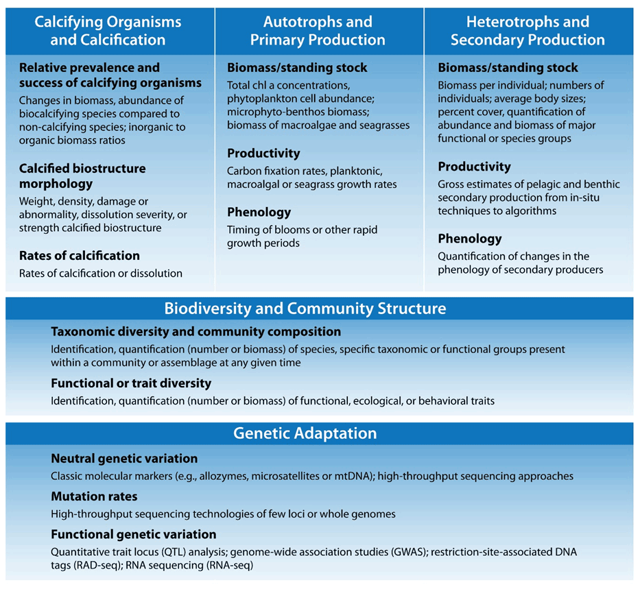
Figure 1 Five fundamental ecosystem traits identified as potentially sensitive to ocean acidification and their observable indicators.

3 Five traits that are influenced by OA

Based on previously published meta-analysis and reviews (e.g., Doney et al., 2020; Figuerola et al., 2021; Hancock et al., 2020; Kroeker et al., 2013; Turley and Gattuso, 2012), we delineate five fundamental ecosystem traits and their suite of observable indicators (Fig. 1): (1) calcified organisms and calcification, (2) autotrophs and primary production, (3) heterotrophs and secondary production, (4) biodiversity and community structure, and (5) genetic adaptation. The specific choice of indicator at different sites will depend on the questions or concerns of the investigator but should relate to fitness of species and the health of marine populations and communities; if relevant, it should also be associated with key ecosystem services. The feasibility of obtaining these observations over the long term must also be considered. Detection of OA-induced change in these indicators hinges upon the variability of the data, so a first step is to apply recognized best practices for biological measurements (Katsanevakis et al., 2012; Bean et al., 2017). Even so, natural “noise” of the system, in terms of short-term environmental changes (weather) and organismal plasticity, must also be taken into account when selecting indicators because it strongly influences the time of emergence of long-term trends (Vargas et al., 2017, 2022).

The specific biological observations listed in this section are examples of potential parameters to measure and are not exhaustive. They provide a suitable framework on which to build both intensive and pragmatic field observation programs that are best suited for local capacities and funding. These methodological inventories will undoubtedly evolve as future technologies emerge and become more widely available over the coming decades (Bean et al., 2017), but the central ecosystem traits they manifest, combined with high-quality carbonate system data, will enable quantification of OA-driven changes in marine ecosystems. The goal is to determine the relationship between rates of chemical and biological changes, enabling comparisons of those relationships across diverse and geographically distributed ecosystems.

3.1 Calcified organisms and calcification

3.1.1 Rationale

The use of calcium carbonate (CaCO₃) structures for structural support and protection is widespread amongst marine organisms (e.g., Monteiro et al., 2016; Fitzer et al., 2019; Clark et al., 2020). As changes in seawater chemistry have been demonstrated to affect calcium carbonate structures and biomineralization rates (see references in Fitzer et al., 2019), analysis of effects from acidification on calcifiers is perhaps the most documented of OA biological impact studies (e.g., Hofmann et al., 2008; Vézina and Hoegh-Guldberg, 2008; Wittmann and Pörtner, 2013; Bednaršek et al., 2014, 2017, 2021a; Osborne et al., 2020). OA can affect the ratio of calcifiers to non-calcifiers in an ecosystem, aspects of calcified structures, and measured rates involving calcium carbonate, including both the deposition and dissolution of calcium carbonate (Fitzer et al., 2019).

3.1.2 Indicator categories and observations

Biomass, abundance, and percent cover of calcifying organisms within an ecosystem

Changes in biomass, abundance, and percent cover of biocalcifying species, compared to non-calcifying species, measured across either fine scales (meters) or broad scales (kilometers) can be used as a primary indicator of OA stress once other known factors are ruled out (e.g., eutrophication). Inorganic to organic biomass ratios (PIC : POC) of individual organisms, populations, or whole assemblages can also provide a sensitive measure of relative changes in the presence of biocalcifying organisms within an ecosystem (Thomsen et al., 2010).

Skeletal morphology and composition

The state, structure, and mineral composition of calcified biostructures yield information about the ability of organisms to maintain the balance of calcification over dissolution and are thus indicators of biological stress. Calcified structure morphology or function can be assessed through measures such as weight, density, damage, porosity, abnormality, dissolution severity, or strength (e.g., Bednarsek et al., 2017, 2021a; Osborne et al., 2020).

Rates of calcification

Calcifying conditions in benthic habitats can undergo large shifts over short (hourly, diurnal) timescales related to physical forcing (e.g., tides, light levels). Measured rates of calcification or dissolution on organismal to ecosystem scales help to discern short-term (semi-instantaneous) responses of biocalcifying organisms to present conditions (e.g., Goreau, 1959; Cohen et al., 2017; Schoepf et al., 2017). These can be accomplished at larger scales with water-mass tracking of observed changes in TA and DIC (along with T, S) to estimate net community calcification (Fitzer et al., 2019), but also at organismal scales with in situ approaches (Melzner et al., 2010; Dellisanti et al., 2020).

3.2 Autotrophs and primary production

3.2.1 Rationale

Primary production, in all of its myriad forms, serves as the foundation for marine ecosystems. Quantifying its susceptibility to OA is crucial because primary production ultimately provides the energy for all trophic levels to adjust to OA-induced stress. Increasing CO₂ can modulate primary production in confounding ways. OA shifts the carbonate system to yield higher pCO₂(aq), which is a fundamental fuel for photosynthesis that often becomes limiting in high-productivity systems (Beardall et al., 2009). Many primary producers (but not all) initiate metabolically costly carbon-concentrating mechanisms that divert energy from growth and reproduction. So, increases in pCO₂(aq) then have the potential to stimulate carbon fixation rates in pelagic and benthic primary producers (Raven et al., 2014), including in marine animal–algal symbioses (Dupont et al., 2012). However, decreasing external and cytosolic pH can disrupt a broad suite of physiological and biochemical factors, including proton pumps, cellular membrane potential, enzyme activity, and energy partitioning (Beardall and Raven, 2004; Giordano et al., 2005). OA may also influence the chemical availability of essential micronutrients (e.g., trace metals, Gledhill et al., 2015), thereby potentially affecting the nutritional support of primary production in some coastal and offshore waters (Hutchins and Boyd, 2016). Another mode of potential impact is that transmembrane proton gradients regulate flagellar motion and thus cell motility (Manson et al., 1977), so OA may reduce the access of vertically migrating flagellated phylogenetic groups to nutrients while simultaneously increasing their susceptibility to predation (Hallegraeff et al., 2012). Despite the likely complexity of potential OA effects on autotrophs and primary production, the responses will be underlain by three chief indicators.

3.2.2 Indicator categories and observations

Biomass and abundance

The total biomass of primary producers in pelagic and benthic environments is often used to signal the energy available for transfer to higher trophic levels (Pauly and Christensen, 1995; Brown et al., 2010). Although methods for quantifying biomass or standing stock vary depending on the environment or organism of interest, they can include measures of total chlorophyll a (chl a) concentrations, phytoplankton cell abundance, microphytobenthos biomass (e.g., chl a per area of surficial sediments), and the biomass of macroalgae and seagrasses. A central benefit of this metric is that it is less susceptible to interannual variability and thus gives more time-integrated insight into the status of communities and regions.

Productivity

Lower levels of biomass at times can mask high carbon turnover rates, so measuring carbon fixation rates or planktonic, macroalgal, or seagrass growth rates can provide more sensitive and comprehensive insight into energy flows in the system (Eddy et al., 2021). In some cases, whole community production rates can be estimated by measuring net carbon and oxygen dynamics (e.g., Juranek and Quay, 2005). However, such estimates are prone to variability at hourly, weekly, and seasonal intervals. Establishing trends associated with OA will require longer time series.

Phenology

Any change in the rates of primary production will alter nutrient dynamics, so it will be important to measure the timing of blooms or other rapid growth periods. If these shifts in phenology become significant, they can lead to temporal disconnect between the timing of high primary producer biomass and sensitive (e.g., larval) life cycle stages of secondary producers that depend upon this energy source (Yamaguchi et al., 2022).

3.3 Heterotrophs and secondary production

3.3.1 Rationale

There is good evidence that long-term exposure to elevated pCO₂ levels increases metabolic energy demand in many marine organisms (e.g., Stumpp et al., 2011; Pan et al., 2015; Jager et al., 2016). This additional energy is needed to support increased acid–base balance activities (e.g., increased cellular proton pump activity to counter acidosis of intracellular fluids) (e.g., Stumpp et al., 2012), increased calcification to counter increased calcium carbonate dissolution (e.g., Ventura et al., 2016), and increased physical activities (e.g., increased burrow ventilation) (Donohue et al., 2012). These additional energy expenditures leave less energy available to invest in other key processes, including protein synthesis and growth. Conversely, any increase in energy demands may be alleviated in part or wholly by increased food supply from CO₂-enhanced primary production, leading to overall increases in heterotroph populations and productivity and thereby changes in ecosystem function. For humans, reductions in marine secondary production may have profound implications for fisheries and aquaculture.

3.3.2 Indicator categories and observations

Biomass, abundance, and percent cover

The total biomass or standing stock of secondary producers in pelagic and benthic environments is not only a sentinel of the available energy transfer upwards into food webs, but also serves as a top-down integrated measure of effective primary production, i.e., autotrophic growth utilized by grazing versus that produced by noxious, toxic, or unpalatable autotrophs. The total heterotrophic community abundance, ideally quantified as biomass per individual but also as numbers of individuals, average body sizes, or percent cover (e.g., sponges, colonial organisms), should be quantified to estimate total heterotrophic biomass on appropriate seasonal or annual timescales. Splitting the quantification of abundance and biomass into major functional or species groups can provide greater detail and resolution for identifying those aspects of the community or ecosystem that are most affected.

Productivity

As with primary producers, the observed biomass or standing stock of secondary producers can be the consequence of rapid or more sluggish growth and predation cycling, so quantifying the rates of secondary production at either community or species scales provides important additional insights into change within environments. There is a wide range of methodologies to calculate gross estimates of pelagic and benthic secondary production from in situ techniques to algorithms (Brey, 2012). It may be useful to emphasize the observation of selected heterotrophic taxa that play a strong structuring role within the local ecosystem or that have high cultural or commercial value. Through its integrative nature, the estimates of secondary productivity are likely to exhibit less temporal variability than that of primary productivity, although the metrics of biomass or standing stock are still the preferable indicator for establishing OA-induced effects on heterotrophs and secondary production.

Phenology

Most marine secondary producers have planktonic life stages that are coupled to environmental cues which signal food abundance (e.g., temperature, light), but this pairing may fail if OA-driven shifts in primary production become substantial. The same may be true for other segments of the food web (e.g., migration patterns of higher organisms). As with primary producers then, quantifying any changes in the phenology of secondary producers will be important for assessing the potential influence of OA on marine ecosystems (Calbet et al., 2014).

3.4 Biodiversity and community structure

3.4.1 Rationale

Many of the processes mentioned in the previous paragraphs result in changes in biodiversity and community structure. There is compelling evidence that the sensitivity of marine organisms to all aspects of OA varies enormously among species (Wittmann and Pörtner, 2013; Vargas et al., 2017, 2022). This variability is created via the combination of different physiological and ecological traits exhibited by the different taxa. Such interspecific variability could allow OA to act directly as a strong selective pressure (Kroeker et al., 2010, 2013; Hancock et al., 2020; Figuerola et al., 2021), decreasing biodiversity directly through species loss (Hall-Spencer et al., 2008; Enochs et al., 2015) or indirectly through a host of processes, such as disrupting competition (e.g., space occupation or resource allocation) or trophic interactions (e.g., predation and grazing; Kroeker et al., 2013b; Vizzini et al., 2017), decreasing energy generation and flow, degrading critical biogenic habitats, or increasing susceptibility to pathogens and diseases (Bibby et al., 2008; Widdicombe and Spicer, 2008; Sunday et al., 2017). Evidence from the paleontological record supports this assumption, with large species extinctions and biodiversity losses being associated with periods of extreme climate change events (Twichett, 2007).

3.4.2 Indicator categories and observations

Taxonomic diversity and community composition

This represents the manifestation of all the direct and indirect impacts acting upon all of the individuals within a community. It is an established metric used in many existing marine monitoring programs and impact assessments. The essential observations to be made are to identify and quantify (number or biomass) the species present within a community or assemblage at any given time. From abundance and biomass data on these species, it is possible to calculate a wide variety of indices, each focusing on specific aspects of community structure and biodiversity (e.g., community abundance and biomass, species richness, evenness, taxonomic relatedness; Gaston and Spicer, 2004). This approach is applicable to all types of communities, including microbial assemblages. Whilst identification of individuals to the species level is desirable, this is not always possible; however, identification at lower taxonomic resolution still allows the relative effects of OA to be assessed on specific taxonomic or functional groups.

Functional or trait diversity

Similar to taxonomic biodiversity metrics described in the previous section, metrics of functional or trait diversity again require the collection of species abundance and biomass data as detailed above. However, in this instance individual organisms are grouped, not by their taxonomic relationships, but by their shared functional, ecological, or behavioral traits. The same biodiversity metrics as used for describing taxonomic diversity can then also be applied to these aggregated data to generate estimates of functional or trait diversity. The benefit of this approach is that it provides information on the potential function and performance of ecosystems and is particularly employed in the study of microbial biodiversity (Krause et al., 2014).

3.5 Genetic diversity

3.5.1 Rationale

Understanding the impact of OA on marine biodiversity requires not only characterizing how these changes will affect ecosystems, but also how populations will respond via acclimation and adaptive evolution (Sunday et al., 2014). OA is an important driver of phenotypic (e.g., morphology, physiology, life history, and even behavior) (Kroeker et al., 2013) and genetic change (functional and structural) (e.g., de Wit et al., 2016; Lloyd et al., 2016). OA is therefore an important component of natural selection. The selective effects of OA can influence micro-evolutionary dynamics by altering demographic parameters (Bramanti et al., 2015), genetic diversity (Lloyd et al., 2016), and the molecular regulation of functional pathways (de Wit et al., 2016; Runcie et al., 2016) in marine organisms. Every species and population has an adaptation potential to OA that is mostly dependent on genetic diversity (Sunday et al., 2014). Characterizing the present level and rate of changes in relevant aspects of genetic diversity is key to understanding the future of marine ecosystems. While this signature can be specific to OA, the signal can vary in strength and direction across temporal and spatial scales depending on the particular genetic and environmental backgrounds of natural populations (Pespeni et al., 2013; Calosi et al., 2017; Gaitan-Espitia et al., 2017).

Progress in high-throughput sequencing technologies allows rapid, cost-effective, and informative measurements of molecular genetic variation (functional and neutral) in natural populations. These techniques have the potential to track, assess, and disentangle the specific OA signature at the molecular level and estimate the rate of micro-evolution in response to OA across population and species.

3.5.2 Indicator categories and observations

Neutral genetic variation

OA can negatively impact nonfunctional genetic variation in marine organisms (Lloyd et al., 2016; Bitter et al., 2019). Indicators of these effects can be estimated from population genetic parameters such as the number of alleles, heterozygosity, effective population size, inbreeding, and population divergence (Schwartz et al., 2007). This assessment can be achieved using classic molecular markers (e.g., allozymes, microsatellites, or mtDNA) or through high-throughput sequencing approaches (e.g., Lloyd et al., 2016; Bitter et al., 2019).

Functional genetic variation

Identifying and monitoring variation in ecologically important and heritable phenotypes traditionally involves the assessment of quantitative, functional genetic variation (Charmantier et al., 2014). For this, different approaches can be used, including quantitative trait locus (QTL) analysis, genome-wide association studies (GWAS), genome scan via restriction-site-associated DNA taqs (RAD-seq), and RNA sequencing (RNA-seq). Linkage and association mapping approaches (QTL and GWAS) allow the identification of regions of the genome that contribute to phenotypic variation and divergence among populations (Savolainen et al., 2013). Similarly, RAD genome scans can affordably and efficiently identify (i) candidate loci underlying local adaptation, (ii) signals of selection across the genomes and species range, and (iii) neutral and non-neutral genetic variation (Lowry et al., 2017). It is important to highlight here that functional genetic variation is not only related to structural differences in protein-coding loci but also in regulatory sequences that influence gene expression (Whitehead and Crawford, 2006). Therefore, approaches such as RNA-seq can help to identify candidate loci and regulatory pathways involved in phenotypic responses to OA across spatiotemporal scales, as well as the mechanisms underlying phenotypic divergence, local adaptation, and phenotypic plasticity in natural populations.

Mutation rates

Mutations are fundamental to evolution as they provide the ultimate source of novel and heritable variation on which selection can act. Thus, assessing mutation rates in natural populations allows us to infer ecological (e.g., population dynamics) and evolutionary (e.g., adaptation) responses of marine organisms to climate change factors such as OA (Collins et al., 2020). In short-living organisms, drastic changes in environmental conditions can induce strong selection, driving rapid evolutionary change (sometimes as few as two generations) as a result of increases in the frequency of rare existing beneficial genetic variants or the generation of new beneficial mutations (Schaum et al., 2018). Estimates of mutation rates can be obtained from few loci (including genes of particular interest) or from whole genomes using high-throughput sequencing technologies. In both cases, molecular variants can be screened among individuals and populations in order to identify candidate genetic changes (de novo mutations and/or existing mutations) that might contribute to the ecological and evolutionary responses to particular environmental conditions such as OA (Schaum et al., 2018; Krasovec et al., 2020). This association between molecular variants such as single-point mutations and the fitness of the organisms can be tested experimentally (e.g., Schaum et al., 2018; Waldvogel and Pfenninger, 2021), linking geno- and phenotypes in evolving populations. This linkage could be achieved using traditional physiological experiments or by measuring the effects of the mutations on gene expression. Finally, mutations can be placed into a functional context by annotation of the protein sequences that host molecular variants using public databases such as the National Center for Biotechnology Information (NCBI) GenBank and the European Nucleotide Archive (ENA) (e.g., Mock et al., 2017).

Figure 2 Within each of the five proposed biological impact indicator categories (calcification, primary production, heterotrophic production, biodiversity, adaptation), it is possible to combine the data from numerous individual time series stations in order to compare the rates of chemical change with the rate of biological change across different geographical locations and between different biological contexts. Each individual data point on the graph represents the summary information from a single time series that has coupled biological impact and carbonate chemistry observation data. With enough observations, it is possible to generate a generic relationship (blue line). Using the relative positions of data points on this plot it is possible to derive site-specific information about the relative importance of OA in driving biological change at the individual time series stations. In scenario 1, the biological impact is largely caused by other environmental drivers, or the biological parameter that was measured is highly sensitive to OA. In scenario 2, the measured biological impact parameter is not sensitive to OA, or the biological impact is being mitigated by other environmental drivers or biological processes.

4 Using “rates of change” to compare in situ observations of biological impact and OA trends to allow regional and global comparisons

Monitoring any one of the parameters described above, over a period of time and in combination with coupled environmental data that include at least two carbonate chemistry parameters, will allow the observer to better describe how their specific measured biological trait is changing in response to ocean acidification. In essence, by calculating and then comparing the rate at which the biological parameter is changing with the rate at which ocean acidification is occurring will identify how closely correlated they are with each other. Such information will augment experimental studies that identify mechanisms by which OA would act upon a biological process to generate a better conceptual understanding of how biological responses to OA will manifest themselves in the field. By the inclusion of other potentially important environmental parameters, such as hypoxia, temperature, and pollution, it will also be possible to see how important OA is in driving biological response compared to the other environmental stressors for that particular biological trait. However, the overall purpose, and greater benefit, of increasing the volume of OA biological monitoring is to collectively use these data together in order to scale up site-specific observations and to thereby understand OA impacts within and across species and populations, geographical locations, and complex environments. For example, analyses could bring together multiple time series datasets to understanding which specific elements of a trait are most affected, whether there is spatial and/or geographical variability in the responses observed, and what the key confounding drivers or processes are that influence the biological response of organisms to OA. Below we outline just one simple methodology for combining data gathered from different parameters and indices within a trait in order to achieve such a holistic overview of trait response. We appreciate that there are other more sophisticated data analysis techniques available, and undoubtedly new ones will evolve in the future. For now, we present this simple method to illustrate a way in which the data we are advocating should be collected and can easily be used to support greater understanding of OA's biological impacts.

As the volume of information on the biological impact of OA has grown, there have been various efforts to synthesize this available knowledge and provide tools for meaningful comparisons among ecosystems and locations. For example, several approaches have been used to synthesize the literature on experimental biological studies including meta-analyses (e.g., Kroeker et al., 2013; Busch and McElhaney, 2016; Bednarsek et al., 2019) and semi-quantitative reviews (e.g., Wittmann and Pörtner, 2013). These approaches largely compare measurements of “effect size”, whereby all observed responses are represented as the relative change from a defined baseline or control condition specific to that observation (e.g., Kroeker et al., 2013). Whilst this approach overcomes the initial problem of data comparability, it still relies on assumptions that effect sizes are roughly representative of biological or ecological consequence. Whilst we acknowledge that further work will undoubtedly be needed to fully understand the ecological consequences associated with different scales of effect size and how this will change depending on the biological process being considered, the basic principle of using effect sizes to compare across different indices remains useful.

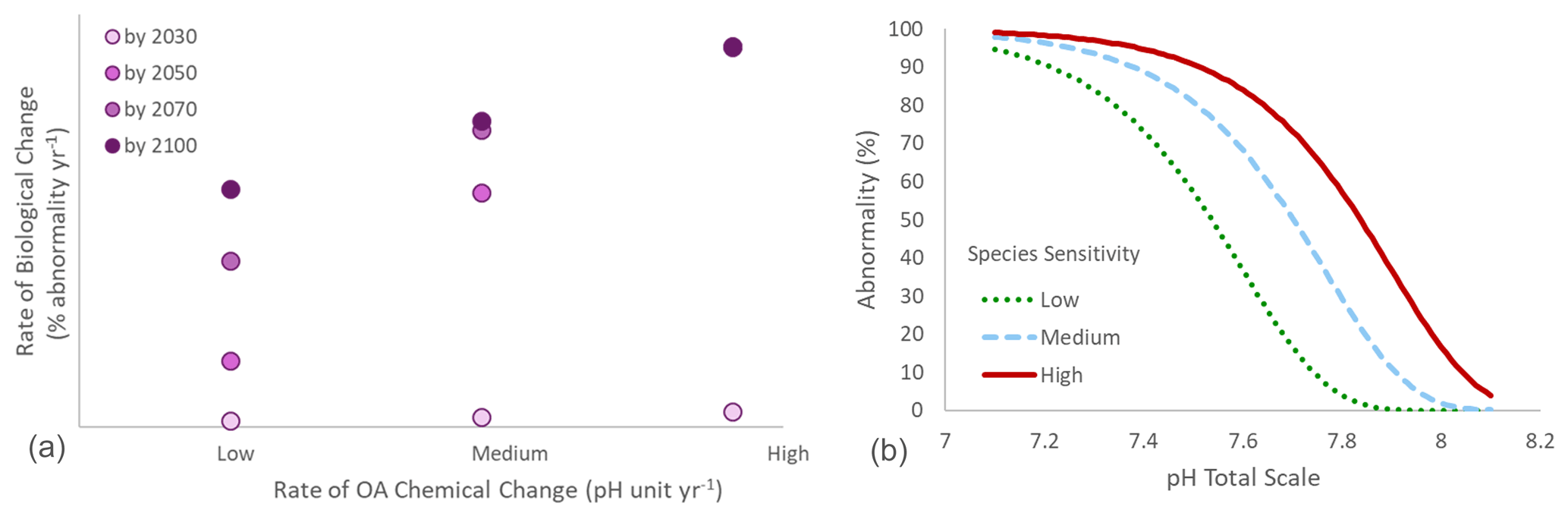
Figure 3 (a) Conceptual relationship between the rate of chemical change (e.g., pH units per year) and the rate of biological change (e.g., percent of change per year) under three different scenarios of rates of chemical change (low, medium, and high). Rates of chemical and biological changes are positively correlated. The rates of biological change calculated by 2100 are compared with rates calculated after 10, 30, and 50 years of observation. After 10 years, the rate of biological change is dramatically underestimated compared to the rate observed by 2100. Under a low rate of chemical change, the rate of biological change is still underestimated after 50 years of observation. Under high chemical rates of change, similar biological rates of change can be calculated after 30, 50, and 80 years of observations. (b) Relationship between pH and larval abnormality (%) in three hypothetical organisms with different sensitivity: low, medium, and high, with tipping points reached at pH 7.6, 7.75, and 7.9, respectively. The medium scenario is based on the mussel Mytilus edulis (from Ventura et al., 2016).

At any given location, we propose that biological observations can be transformed into an effect size (e.g., in percent) relative to a given reference time, and modeling the evolution of this effect size through time allows the calculation of a rate of biological change as the total percent change in the biological process divided by the time over which that change happened. We propose that quantifying the relationship between these rates of biological change and the rates of chemical change associated with OA is an effective way to assess the influence of that OA on the biological change observed. At any given location, this approach would thereby provide information on the risks and vulnerabilities associated with OA. A comparison of rates of change of specific chemical and biological indicators will also help in building a mechanistic understanding of the relationship between changes in relevant carbonate parameters and biological processes (e.g., Osborne et al., 2019). More importantly, it would allow comparison among overall biological responses across a wide range of locations.

As a general principle, in situations in which OA is the primary driver of a biological response, the rate of that biological change is expected to be closely correlated with the rate of chemical change. The precise nature of this relationship (i.e., the direction and slope magnitude) will also depend on the sensitivity of the process, organism, or ecosystem: at a given rate of chemical change, a sensitive organism is expected to show a stronger biological response than a less sensitive one. The rate of biological change is then the product of the interaction between biological sensitivity and rate of chemical change. By plotting together data from various long-term studies, with each time series of biological and chemical observations represented on a plot by a single point (defined by the rate of biological change on the x axis and the rate of chemical change on the y axis), it is possible to compare across different studies to define a generic relationship between OA and a specific biological trait (Fig. 2). While we use a linear relationship between the chemical and biological rates of change as an illustration in the Fig. 2, the precise nature of this relationship may follow other patterns such as a nonlinear tipping point response (e.g., Wunderlink et al., 2021).

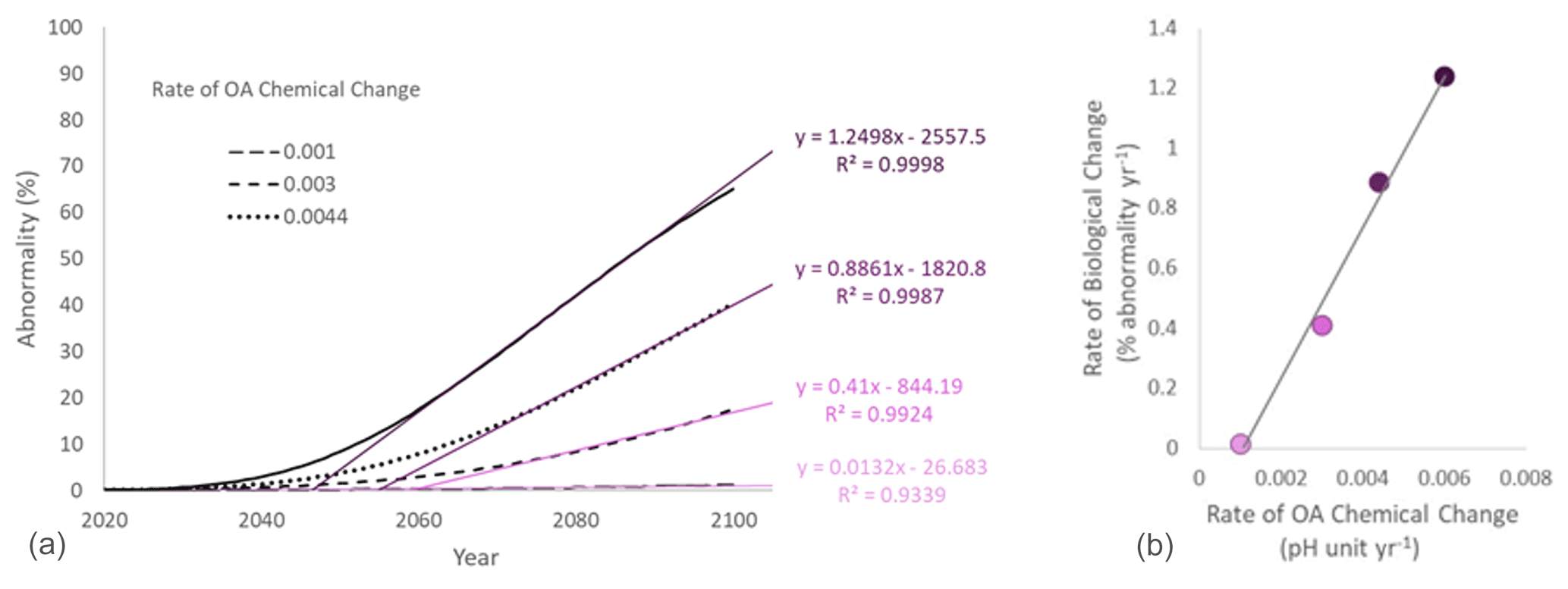
Figure 4 (a) Projection of larval abnormality under different scenarios of rate of chemical change. The rate of biological change was estimated for each scenario as the coefficient of the significant regression between time and abnormality (%) over the linear phase of the curve. (b) Relationship between the chemical and the biological rates of change.

It is important to remember that OA will not be the dominant driver at all locations. For example, a sensitive species exposed to a low rate of chemical change may lead to a lower rate of biological change than a more tolerant species exposed to a high rate of chemical change. Such deviations from the generic relationship would therefore identify locations where other biological drivers play a more important role or amplify (scenario 1 in Fig. 2) or mitigate the effect of OA that is being investigated (scenario 2 in Fig. 2). Furthermore, those deviations could highlight situations in which the specific biological parameter measured was more or less sensitive to OA than others: for example, observations of calcification rate may all appear above the generic relationship line, while observations of shell mass may all appear below the line. Both of these parameters (calcification rate and shell mass) provide information on the calcification process, but their relative positions on the plot would indicate differences in the mechanisms by which OA impacts those particular biological indices.

5 Points to consider when comparing the impacts of OA on biological traits derived from different observations and different places

To be meaningful and useful in the analysis proposed above, observed rates of biological change must be robust. If calculated with too few data, these rates can severely underestimate the real impacts. One of the key questions when evaluating an OA biological observation time series is how long that time series needs to be to ensure that rates of change have been accurately quantified. The minimum duration of observation is largely dependent on both the specific sensitivity of the organism or ecosystem being observed and the underlying rate of chemical change. This concept is described theoretically in Fig. 3a, which shows that the longer the data are collected for, the more likely they are to provide an accurate estimate of the rate of change over that time period. However, under higher rates of chemical changes, robust estimates of the rate of biological change can be obtained over a shorter period of time. This illustrates the importance of backing up monitoring observations with targeted studies that can approximate the likely sensitivity of biological processes and parameters to OA stress. For example, generating a performance curve can provide an illustration of the effect of a given parameter (e.g., pH) on a biological response. Relationships between a stress and a biological response are often not linear and can be measured under laboratory conditions for a given species and location (e.g., Ventura et al., 2016). These curves can then be used to provide estimates of the minimum duration of a biology monitoring program under different rates of chemical changes to properly quantify the rate of biological change.

Here we use real data to illustrate the point. The performance curve between pH and larval abnormality was experimentally measured for the blue mussel Mytilus edulis population from the Gullmarsfjord in Sweden (Ventura et al., 2016; medium sensitivity on Fig. 3b). The present average pH in surface seawater in the Gullmarsfjord is 8.1 (Dorey et al., 2013). Rates of pH change ranging from 0.001 (slow change corresponding to a decrease by 0.08 pH units by 2100) to 0.006 pH units of decrease per year (fast change corresponding to a decrease by 0.48 pH units by 2100) were compared. These rates were used to estimate the pH at any given time, and the associated abnormality was calculated using the performance curve adapted from Ventura et al. (2016) (Fig. 4a). For each scenario of rate of chemical change, the rate of biological change was calculated as the slope of the significant linear regression between time and abnormality (%) over the linear phase of the curve. Ideally, the rate of biological change should be calculated using a nonlinear model following the shape of the nonlinear performance curve between pH and the tested parameter (e.g., Fig. 3b for percent of abnormality). These performance curves can take many forms depending on the measured parameter and species. For example, common shapes of physiological performance curves include U shape, sigmoidal, logarithmic, exponential, and inverted U shape (Little and Seebacher, 2021). However, in practice the shape of these curves is often unknown and it would not be possible to derive relevant rates of change from biological observations over a relatively short period of time. Under these circumstances, using a linear regression is a good alternative. From the projections using the blue mussel data, we observe a linear relationship between rates of chemical and biological change. In other words, for a given organism at a given location, the rate of biological change increases with the rate of chemical change (Fig. 4b).

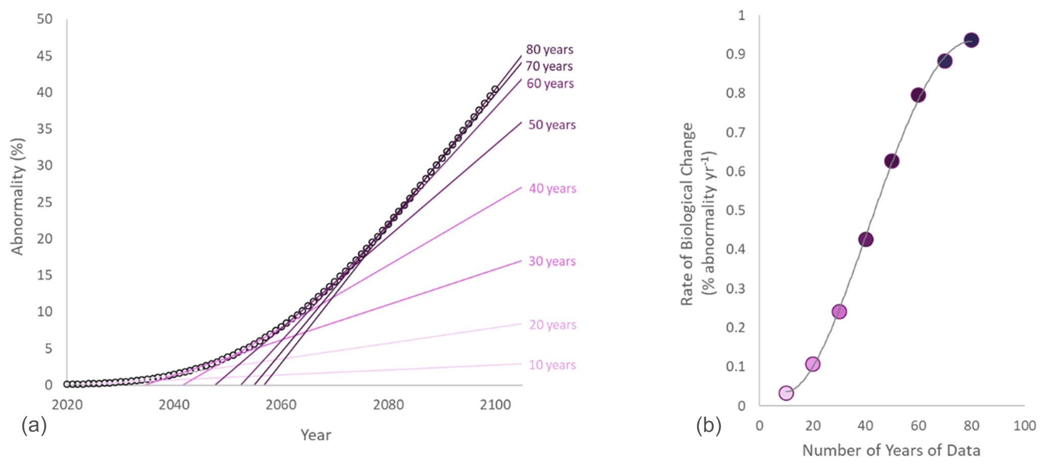
Figure 5 (a) Evaluation of the rate of biological change as the coefficient of the significant regression between time and abnormality over time (after collecting 10 years of data, 20 years of data, etc.). (b) Relationship between the number of years of data for the biological monitoring and the calculated rate of biological change.

It is then possible to use these data to estimate the number of years of observations to detect a negative impact. In the region where the mussels were collected, the current rate of chemical change in surface water is estimated as a decrease of 0.0044 pH units per year, corresponding to a decrease of 0.35 pH units by 2100 (Andersson et al., 2008). Based on our model, this would lead to an observed rate of biological change of 0.8861 % of abnormality per year by 2100 (Fig. 4). Using this model, it is possible to quantify the evolution of the rate of biological change over time (Fig. 5a) and then estimate how many years of observations are needed to calculate a good estimate. The rate of biological change increases with increasing years of observations (Fig. 5b). As a consequence, biological monitoring over a short period of time leads to an underestimation of the rate of biological change. For the mussel M. edulis in the Gullmarsfjord and under a realistic rate of chemical change, we can then estimate that at least 70 years of biological monitoring would be needed to calculate an accurate rate of biological change.

It is worth noting that in the example presented above, the subject species was considered to be relatively insensitive to OA, resulting in a need for many decades of monitoring. For more sensitive biological subjects and processes in areas of more rapid chemical change, the required length of observations will be much shorter. It is also important to note that other parameters or stressors, short-term variability, ecology, and evolution can modulate the biological response and then influence the rate of biological change. As an example, we compared rates of biological changes in three “hypothetical model” organisms with different levels of sensitivity to pH (Fig. 3b). This scenario could represent different populations of the same species adapted to different levels of pH variability (e.g., Vargas et al., 2017, 2022) or with different modulating factors (e.g., temperature or food concentration) or evolution of the performance curve within one population through time as a consequence of transgenerational adaptation or evolution (Parker et al., 2015; Thor and Dupont, 2015; De Wit et al., 2016). Assuming a rate of chemical change of 0.0044 pH units per year (Andersson et al., 2008), the rate of biological change observed by 2100 would be dependent on the species sensitivity (Fig. 6a).

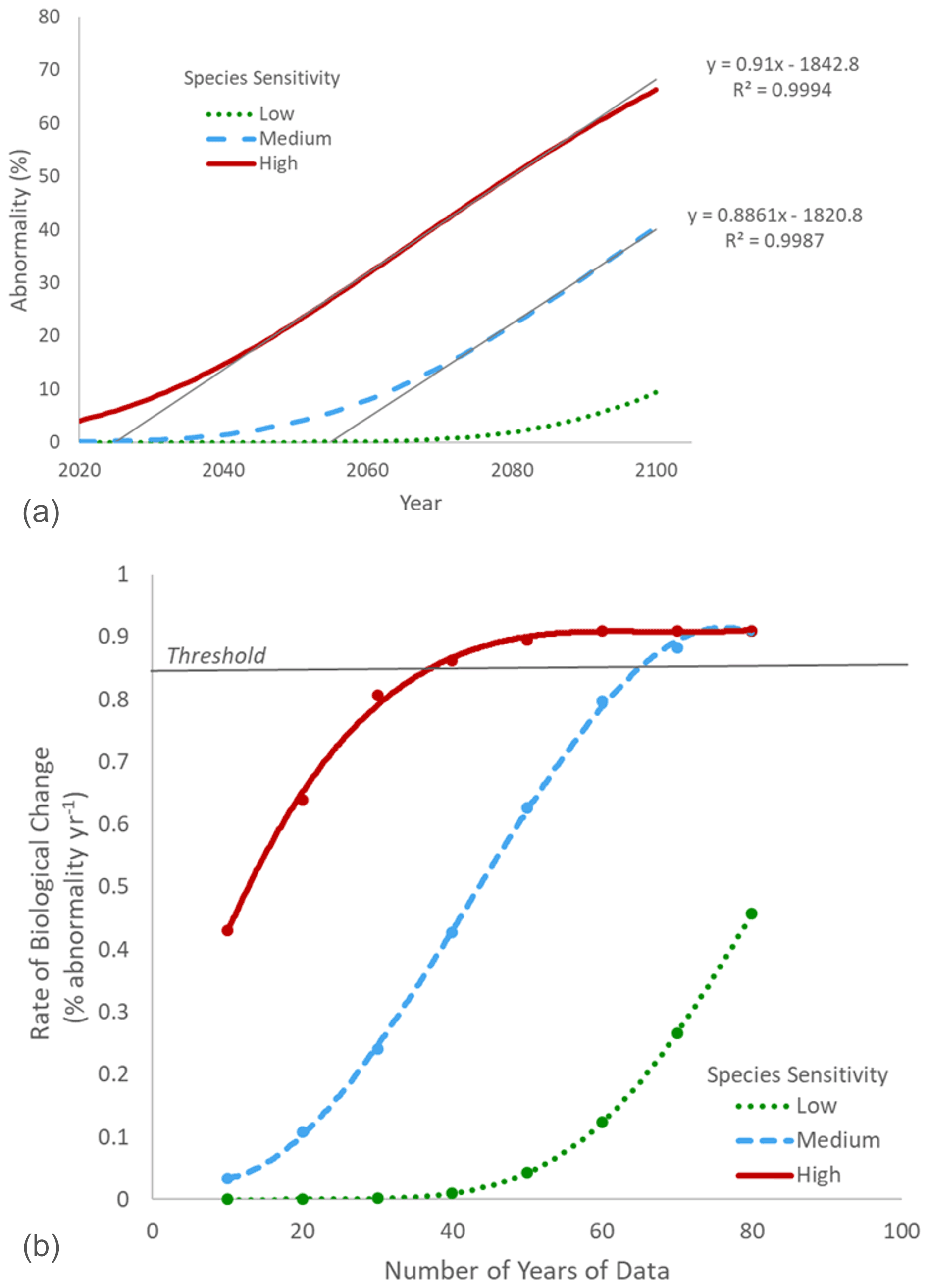
Figure 6 (a) Projection of larval abnormality under a rate of chemical change of 0.0044 pH units per year (Andersson et al., 2008) for organisms with three different levels of sensitivity to pH (low, medium, high). The rate of biological change was estimated for each scenario as the slope of the significant regression between time and abnormality (%) over the linear phase of the curve. For the species with low sensitivity, the linear phase was not reached, and it was not possible to calculate the rate of biological change. (b) Relationship between the number of years of data for the biological monitoring and the calculated rate of biological change for three organisms with different levels of sensitivity to pH (low, medium, high). Sufficient years of data were considered to have been collected when the observed rate of biological change was above the 0.86 threshold (5 % from the maximum rate of change of 0.91 % of abnormality per year).

For each level of sensitivity, it is possible to estimate the minimum number of years of observation needed to calculate an accurate rate of biological change (with a 5 % error; Fig. 6b). As expected, biological monitoring can be shorter for organisms with higher sensitivity to pH. An accurate rate of biological change can be estimated after only 40 years for an organism with high sensitivity compared to 70 years for those with medium sensitivity. For organisms with low sensitivity, the rate of biological change is dramatically underestimated after 80 years. As a consequence, if the purpose of a time series is to calculate a meaningful rate of biological change in as short a time as possible, it is recommended to focus on environments with a high rate of chemical changes and biological indicators that are highly sensitive to OA. However, other sites and processes of high ecological and socioeconomic importance should not be neglected, even if it is likely to take many years for a truly accurate relationship between biological response and OA to appear. It is essential to acknowledge that identifying trends in regions with low rates of chemical change or in organisms with high tolerances to OA may require more time, but that does not mean those impacts do not exist or are of low importance.

Species and population sensitivities are key parameters to consider in the design of a new biological program aiming to document the biological impact of OA. Working with low-sensitivity organisms would lead to a severe underestimation or unrealistically long data collection periods for an accurate estimation of the rate of biological change. As sensitivity can be modulated by several parameters (e.g., evolution) within a population, it is recommended to regularly calculate the rate of biological change and plot it over time. The rate of biological change is expected to increase with time until saturation is reached (Figs. 5 and 6b). At saturation, the rate of biological change can then be considered robust.

Finally, when comparing chemical and biological rates of change, it is also critical to ensure that the spatiotemporal resolution of the carbonate chemistry data is directly relevant for the given species or ecosystem being observed. For example, chemistry data collected in the surface water may not be relevant for a tidal organism experiencing much more variability than that detected by the chemical observations. Similarly, it is important to remember that the carbonate chemistry experienced by a given species is also dependent on its biology. For example, some species migrate over large distances and through very different bodies of water or have different life-history stages living in different environments. Alternatively, some species, mainly sessile, can alter temporal dynamics in the surrounding carbon chemistry through physiological processes such as respiration, photosynthesis, and calcification (e.g., seagrasses, kelp) (Pfister et al., 2019; Unsworth et al., 2012).

6 Conclusions

Assessing the vulnerabilities and adaptive capacity of marine ecosystems and coastal communities towards OA requires a broad range of data. Measurements and calculations related to SDG indicator 14.3.1 (“average marine acidity – pH – measured at agreed suite of representative sampling stations”) provide the chemical information required for such analyses. However, achieving SDG target 14.3 (“minimize and address the impacts of ocean acidification, including through enhanced scientific cooperation at all levels”) will also require correlating those observed chemical changes with the biological response. This immense task can only be accomplished with a combination of approaches including laboratory and field experimentation, modeling, and biological observations. While the body of experimental evidence on OA impacts is growing rapidly, in situ monitoring conducted specifically for identifying and quantifying biological responses to OA is far less common.

Our innovative approach goes beyond the simple monitoring of specified biological traits. We propose a strategy that aims to compare the relationships between rates of chemical and biological change under different circumstances, allowing comparison across regional and global scales. We have shown that identifying robust rates of biological changes over a reasonable time (within a few decades) depends on local species, ecosystem sensitivities, and rates of chemical change and that the interpretation of observed biological responses needs to be mindful of this. We show that it is possible to use performance curves from experimental studies and data from chemical monitoring programs as a first-order step to identify the sites for biological monitoring that will give the most rapid indication of OA impacts, as well as the minimum duration to measure robust rates of biological change. We also propose five fundamental ecosystem traits that optimize the probability of identifying OA impacts: (1) calcified organisms and calcification, (2) autotrophs and primary production, (3) heterotrophs and secondary production, (4) biodiversity and community structure, and (5) genetic adaptation. These traits span all marine ecosystems, are anticipated to be sensitive to OA, and can be quantified using “standardized” biological observations that in many cases are already collected alongside chemical observations. It needs to be highlighted that the specific choice of trait and respective parameters at different sites will depend on local practicalities, specific scientific questions, and envisaged outcomes related to fitness of species and the health of marine populations and communities. The feasibility of obtaining these observations over the long term must also be considered, e.g., access to the marine ecosystem, as well as technical and human scientific capacity.

Selection of sites for biological observations should be based on answering a scientific question or to fit a specific stakeholder need. For example, sites can be selected for a practical reason (e.g., co-location with a long-term chemical observing site or at a marine station facilitating data collection), at a site of particular socioeconomic or cultural value, or scientific interest (e.g., predicted low or high sensitivity to OA). We propose a conceptual framework that would allow bridging chemical and biological monitoring as well as identifying the issues to consider when interpreting the collected data and evaluating the relevance of observed trends. We also argue that meaningful trends can be more rapidly identified at sites combining a high rate of chemical change with high biological sensitivity to changes in the carbonate chemistry. However, this is only one of the many valid reasons to identify a monitoring site, and as OA is only one of the many environmental parameters driving biological changes, other sites should not be neglected.

No single approach can explain the complexity of the biological consequences of OA. Monitoring is the ultimate tool to observe the impact of OA in the ocean, but understanding and addressing the issue will require a combined approach with paleo-investigations, field and laboratory experimentation, and modeling (Dupont et al., 2021). Each of these approaches is associated with its own set of strengths and limitations. Monitoring is realistic but often requires decades of data; experimentation can provide a mechanistic understanding over shorter periods of time but leads to practical limitations in terms of the realism (e.g., single stressors, lack of ecological relevance, short term; Riebesell and Gattuso, 2015). The real strength comes from a combination of approaches. For example, we show that laboratory-based performance curves combined with data from observations of the carbonate system can be used to estimate the duration of a biological observing program to detect meaningful trends. Similarly, data from chemical and biological observations could be combined to evaluate the performance curve of a given species in its natural environment (realized niche) and compare with the curves from the laboratory (fundamental niche).

New data and information obtained when measuring biological indicators alongside chemical changes due to OA will allow the scientific community to contribute to the achievement of the vision of the UN Decade of Ocean Science for Sustainable Development, which involves “the science we need for the ocean we want” (IOC-UNESCO, 2020), as well as its outcomes and objectives. Biological observations assessing the impacts of OA will support several Ocean Decade challenges, in particular Challenge 2, which is to “understand the effects of multiple stressors on ocean ecosystems, and develop solutions to monitor, protect, manage and restore ecosystems and their biodiversity under changing environmental, social and climate conditions”. Furthermore, the implementation and related initiatives of this proposed strategy will be an integral part of delivering the Ocean Decade program “Ocean Acidification Research for Sustainability (OARS) – Providing society with the observational and scientific evidence needed to sustainably identify, monitor, mitigate and adapt to ocean acidification; from local to global scales”. The strategies for biological observing and data analysis presented here offer a vision towards achieving OARS Outcome 4: increase understanding of ocean acidification impacts to protect marine life by 2030. Specifically, by supporting the implementation of an established framework for biological observation set within the existing ocean acidification monitoring framework, the possibility to improve predictions of vulnerability and resilience to ocean acidification at all temporal and spatial scales can be provided. This paper presents a way to unify biological field observations and thereby detect and compare ocean acidification impacts across marine species and ecosystems, thus improving our understanding and knowledge about OA and actively contributing to human well-being (Falkenberg et al., 2020). In doing so, our approach to coupled biological and environmental observations will facilitate greater global connectivity between the collection of physical, biogeochemical, and biological essential ocean variables (EOVs) through the Global Ocean Observing System (GOOS) and essential biodiversity variables (EBVs) from the Group on Earth Observations Biodiversity Observation Network (GEO BON).