the Creative Commons Attribution 4.0 License.
the Creative Commons Attribution 4.0 License.
 | 09 Jun 2022
Data-assimilation-based parameter estimation of bathymetry and bottom friction coefficient to improve coastal accuracy in a global tide model
Martin Verlaan
Jelmer Veenstra
Hai Xiang Lin
Global tide and surge models play a major role in forecasting coastal flooding due to extreme events or climate change. The model performance is strongly affected by parameters such as bathymetry and bottom friction. In this study, we propose a method that estimates bathymetry globally and the bottom friction coefficient in shallow waters for a global tide and surge model (GTSMv4.1). However, the estimation effect is limited by the scarcity of available tide gauges. We propose complementing sparse tide gauges with tide time series generated using FES2014. The FES2014 dataset outperforms the GTSM in most areas and is used as observations for the deep ocean and some coastal areas, such as Hudson Bay and Labrador, where tide gauges are scarce but energy dissipation is large. The experiment is performed with a computation- and memory-efficient iterative parameter estimation scheme (time–POD-based coarse incremental parameter estimation; POD: proper orthogonal decomposition) applied to the Global Tide and Surge Model (GTSMv4.1). Estimation results show that model performance is significantly improved for the deep ocean and shallow waters, especially in the European shelf, directly using the CMEMS tide gauge data in the estimation. The GTSM is also validated by comparing to tide gauges from UHSLC, CMEMS, and some Arctic stations in the year 2014.
- Article
(18600 KB) - Full-text XML
- BibTeX
- EndNote


Accurate prediction of water levels in coastal areas is of significant importance. Coastal flooding, mainly caused by storm surges, is one of the main risks for the world's coastal areas (McGranahan et al., 2007; Kron, 2012). Global exposure to flooding has had an upward trend in recent years due to climate change and sea level rise (Hallegatte et al., 2013; Wahl et al., 2017; Oppenheimer et al., 2019). For example, the global sea level is currently rising at 3–4 mm yr−1, and a 10–20 cm sea level rise would more than double the frequency of coastal flooding before 2050 (Vitousek et al., 2017). This demands global tide and surge models that can provide sea level estimates for large-scale assessments of the flooding risk (Ward et al., 2015).
Global tide models are often divided into three groups, empirical tide models, purely hydrodynamic forward models, and hydrodynamic tide models with data assimilation (Stammer et al., 2014). To study the interaction of tides with other processes such as surge and sea level rise, it is very useful to model tide and surge together in one model. For example, the Global Tide and Surge Model (GTSM) is capable of simulating not only tides but also surges by adding meteorological wind and air pressure forcing (Verlaan et al., 2015). Another application is the provision of boundary conditions for regional models (Zijl et al., 2013). The accuracy of tide and surge models has improved significantly over the past decades through improved physical processes, increased grid resolution, and improved input datasets. For instance, Muis et al. (2017) produced a global reanalysis of storm surges and extreme sea levels (GTSR dataset) from the GTSM and estimated that about 160 million people were exposed to a flood in 2010 occurring once in 100 years. With the improvement of the GTSM in version 3.0, a new dataset called the Coastal Dataset for the Evaluation of Climate Impact (CoDEC) was developed and evaluated as the successor of GTSR (Muis et al., 2020). We will show that a significant part of the remaining uncertainty is caused by uncertainties in the model parameters, such as bathymetry and friction parameters.
This parameter uncertainty can be reduced by parameter estimation. In our view, this is a form of data assimilation (Heemink et al., 2002; Zijl et al., 2013; Mayo et al., 2014). Stammer et al. (2014) reported that assimilated tide models have higher accuracy than non-assimilative models. For example, Wang et al. (2021b) developed an efficient iterative parameter estimation scheme to estimate bathymetry corrections globally for the high-resolution GTSMv3.0 and significantly improved model performance in the deep ocean but improved the performance in shallow water only slightly. To further improve the model accuracy near coastal regions, we propose a combined estimation of bathymetry and the bottom friction coefficient using more observations in coastal areas. Bottom friction plays an essential role at the coasts, accounting for the majority of tide energy dissipation (Egbert and Ray, 2001). The total amount of global tidal energy dissipation is approximately 3.7 TW, and two-thirds is generated by bed stress. The bottom friction term is often modeled in the quadratic bed stress formula. There are several commonly used parameterizations, such as Chézy, Manning, or White–Colebrook (Manning, 1891; Colebrook et al., 1937). The coefficient is often tuned using some model tests that try to reduce the difference between the model and measurements. This value is difficult to set accurately but strongly related to the water level representation in shallow water. Moreover, the bottom friction coefficient can vary strongly between regions.
In regional tide models, data assimilation is applied predominantly to estimate bathymetry, bottom friction, and boundary variables (Navon, 1998; Edwards et al., 2015) with ensemble (Siripatana et al., 2018; Slivinski et al., 2017) or adjoint methods (Zhang et al., 2020). Ullman and Wilson (1998) estimated a drag coefficient by assimilating acoustic Doppler current profiler (ADCP) data into a tidal model of the lower Hudson estuary with the adjoint method. Zijl et al. (2013) improved the water level forecast for the northwestern European shelf and the North Sea through directly modeling and assimilating altimeter and tide gauge data to adjust bathymetry and Manning's roughness coefficient. Mayo et al. (2014) estimated a spatially varying Manning coefficient using an advanced circulation (ADCIRC) model of Galveston Bay with a square root ensemble Kalman filter. The estimation of bottom friction using data assimilation has been applied successfully to the European continental shelf (Heemink et al., 2002) as well as the Bohai, Yellow, and East China seas (Wang et al., 2021a). We found only a few parameter estimation applications at a global scale. Blakely et al. (2022) adjusted the bottom friction and internal tide friction in 41 subdomains to better represent the tide in the ADCIRC model, allowing the bottom coefficient to vary with the subdomain gives a significant improvement on model performance. Lyard et al. (2021) assimilated altimetry tides and tide gauge data into a combination of a time-stepping and spectral tide model. The uncertainty for the model is partly based on parameter uncertainty, such as bed friction, but the result is in the form of 34 tidal components in a gridded data collection with a resolution of , called FES2014. It can provide accurate estimates of tides, but the result is a relatively static dataset because the underlying T-UGO tide model is only used as a first guess or weak constraint. In contrast, we propose a different approach to calibrate the GTSM in this paper using the model as a strong constraint. This results in a calibrated model that can be used as a regular non-assimilative hydrodynamic model. For example, we use the GTSM for storm-surge forecasting and studying the impact of sea level rise; neither is possible with FES2014.
There are considerable differences between data assimilation for tides in deep water and near the coast. In the deep ocean, bathymetry is reported as the parameter that has the most influence on the tide representation (Wang et al., 2021b). The sensitivity to bottom friction is very small in deep water but is often the most sensitive parameter in shallow water. Zaron (2017) highlighted the relative importance of the friction parameter in the momentum balance in the Sea of Okhotsk based on sensitivity test results. The main reason for this is that the effects of both parameters interact. In this study, we combined the estimation of bathymetry and bottom friction. Bathymetry directly controls the tide propagation speed, which is proportional to the square root of the local water depth (Pugh and Woodworth, 2014). On the other hand, bottom friction controls the dissipation of tide energy (Egbert and Ray, 2001). But bottom friction also decreases with depth, which results in a nonlinear interaction. Moreover, due to the quadratic velocity in the friction term, the effect of friction is enhanced when the different tidal constituents propagate along shallow water with complex topography (Cai et al., 2018). Thus, water level is influenced by the co-action of bathymetry and bottom friction. This also creates an interaction between the deep ocean and the shelf. The bathymetry in the deep ocean not only affects the tidal propagation there but also in adjacent coasts. And though the dissipation by bottom friction predominantly occurs in shallow water, this will also change the tides in the adjacent deep ocean when the tide propagates from the coastal regions to the nearby deep ocean. The range of affected areas is related to the topography and tide dissipation (detailed analysis in Sect. 4). To our knowledge, this is the first study with a global model that to combine the estimation of bathymetry and bottom friction in the time series approach. With this approach, we aim to improve modeled tides in both the deep ocean and along the coasts.
We use the computation- and memory-efficient parameter estimation schemes proposed in our previous study (Wang et al., 2021b, 2022). Bathymetry is estimated in all ocean basins, and regions with significant tidal energy dissipation are selected for the bottom friction coefficient estimation. The areas with the most tidal energy dissipation are the Hudson Bay region and European shelf (Egbert and Ray, 2001). FES2014 time series are used as observations for the deep ocean. This dataset has higher accuracy for tides than our initial model (Stammer et al., 2014; Wang et al., 2021b), and with FES2014 tide time series are generated easily for arbitrary locations and periods. In coastal areas, tide gauge data are included in the estimation and validation processes to increase coverage. Tide gauge data were collected from the UHSLC (global coverage), CMEMS (Europe), and tide gauge stations in the Arctic Ocean from Kowalik and Proshutinsky (1994). Since tide gauge data are scarce in some areas, we also investigated the use of FES2014 in some coastal regions. The bottom friction is estimated in the Hudson Bay region, European shelf, and often other regions with large energy dissipation using a combination of FES2014 and tide gauge data as observations. Together, these datasets form a reliable joined parameter estimation application to correct the bathymetry globally and bottom friction coefficient in the coastal and shelf seas, resulting in an accurate hydrodynamic model that can be used for complete tide and surge forecast.
In Sect. 2, the Global Tide and Surge Model (GTSM) and the parameter estimation scheme are introduced. Section 3 describes the strategies for the bottom friction coefficient subdomain specification and the selection of observations. Section 4 presents the parameter estimation experiment setup and results analysis. The estimated model is evaluated with a 1-year-long comparison with the FES2014 dataset and tide gauge data in both the time and frequency domains in Sect. 4. Finally, the discussion and conclusions follow in Sect. 5.
2.1 Global Tide and Surge Model (GTSMv4.1)
We use version 4.1 of the Global Tide and Surge Model(GTSMv4.1) in this study. It is a depth-averaged hydrodynamic model developed in the Delft3D Flexible Mesh with an unstructured grid (Verlaan et al., 2015; Kuhlmann et al., 2011). The model is forced by the tide-generating potential with a full set of tide frequencies. The GTSM is a combined tide and surge model to study some events such as the effect of tropical cyclones and sea level changes on a global scale. Surge is induced by the gradients in the atmospheric surface pressure and the momentum transfer from the wind to the water.
The bathymetry used in GTSMv4.1 is a combination of the General Bathymetric Chart of the Ocean with a 15 arcsec resolution globally (GEBCO, 2019) and EMODnet2018 at 250 m resolution in the European shelf. For consistency between the vertical reference of the model and that of the data, all bathymetric data are corrected using the mean sea level (MSL) as its vertical reference datum. The GTSM has 4.9 million grid cells with a 25 km resolution in the open ocean and 2.5 km in the coastal zone (1.25 km in Europe). We also make use of a coarser grid version of the GTSM (GTSM with the fine grid and GTSM with the coarse grid hereafter). The GTSM with the coarse grid has grid cells of 50 km in the deep ocean and 5 km for shallow waters, resulting in 2 million grid cells. Higher resolution results in better representation of water levels but longer computation times. The CPU time used by the GTSM with the coarse grid is one-third of the fine grid. We use the coarse grid model in the estimation process to reduce the computational cost with the coarse-to-fine strategy. It will be described in more detail in Sect. 2.2.
The GTSM uses a quadratic formulation of velocity and the bottom friction known as the Chézy formula (Manning, 1891):
where ρ is the density of water, and u represents the depth-averaged horizontal velocity vector. In the Chézy formulation, C is the constant coefficient with the value of C=62.5 (m s−1). The bottom friction term is important to determine hydrodynamic conditions and sediment transport processes. Two-thirds of the tide energy dissipation is determined by the bottom friction. When the tide propagates over steep topographies, energy is also dissipated by generation the internal tides. Internal tide friction is parameterized in the formula of the Nycander (2005) tensor scheme.
In comparison to GTSMv3.0 that was used in our previous study (Wang et al., 2021b), GTSMv4.1 contains an updated internal tide friction term that is related to the buoyancy frequency of the stratified ocean. In the previous version of the GTSM, the layer thickness variability was not taken into account properly and this was fixed in the dataset for GTSMv4.1. The correction coefficient for this improved dataset is derived again, and the spatially uniform bottom friction was set to a value found more often in the literature. GTSMv4.1 uses a full set of 484 tide potential frequencies compared to 60 constituents in GTSMv3.0 in our previous study (Wang et al., 2021b). These changes result in a more accurate initial model with the standard deviation (SD) reduced by 1 cm compared to the FES2014 dataset.
(Ray, 2013)(Cheng and Andersen, 2017)(Hart-Davis et al., 2021)(Arbic et al., 2010)(Arbic et al., 2008)(Müller et al., 2012)(Pringle et al., 2021)(Lyard et al., 2021)(Taguchi et al., 2013)(Egbert and Erofeeva, 2002)Table 1Global tide model classification and resolution.
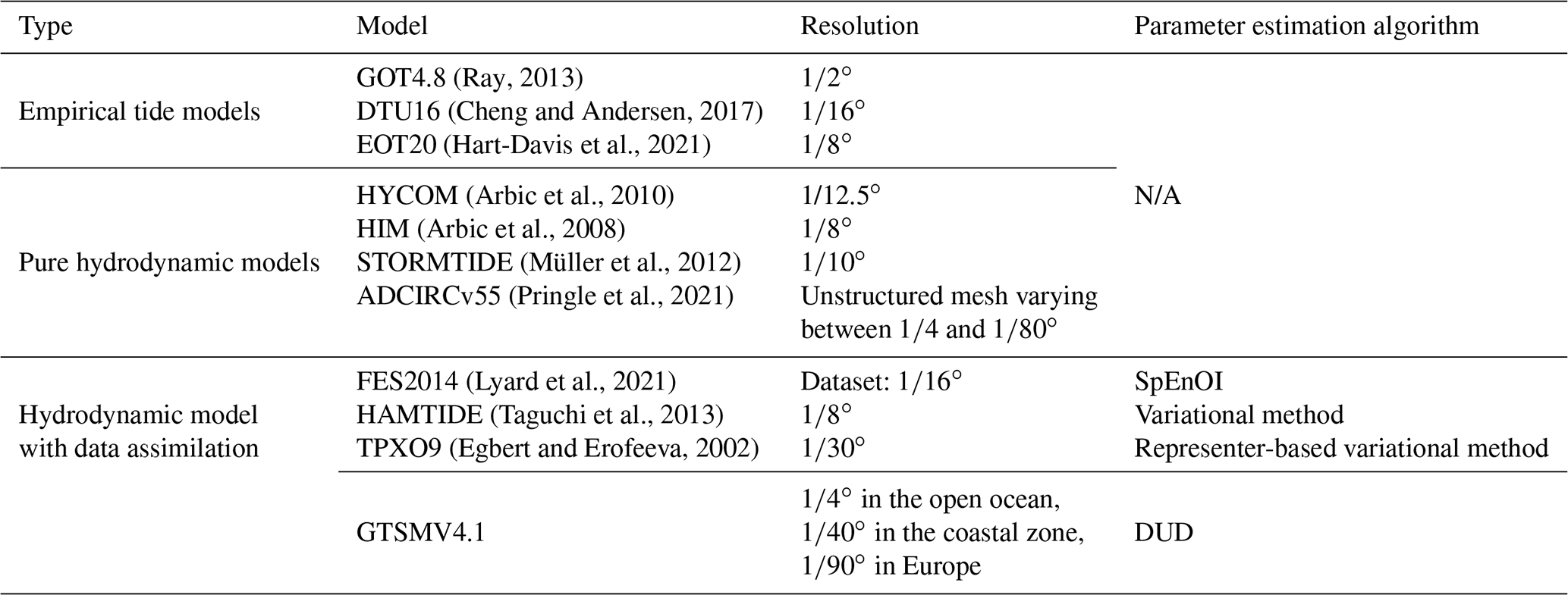
N/A means no parameter estimation is applied to these models.
2.2 Parameter estimation scheme
Global tide and surge models can be classified into three groups, empirical tide models, purely hydrodynamic models, and models with data assimilation, as shown in Table 1. Some parameter estimation algorithms have been applied to global tide models. FES2014 uses the Spectral Ensemble Optimal Interpolation (SpEnOI) algorithm to estimate the bottom friction coefficient, the internal tide drag coefficient, the bathymetry, and the LSA (loading and gravitational self-attraction). It leads to an accurate data collection of 34 tidal components. HAMTIDE is a time-stepping high-resolution tide model corrected by the variational data assimilation algorithm. TPXO9 is a spectral barotropic tide model assimilated using a variational method. However, the spectral tide model cannot exactly compute the tide component interactions, even though some methodologies such as representing the interaction through linearization of the bottom friction term are presented (Provost and Lyard, 1997).
In this study, we use the time–POD-based coarse incremental parameter estimation scheme developed in our previous study (Wang et al., 2021b). The basic algorithm is called DUD (Doesn't Use Derivatives) in the generic data assimilation toolbox OpenDA (Ralston and Jennrich, 1978; OpenDA User Documentation, 2016). DUD is a Gauss–Newton-like algorithm but is derivative-free to solve the nonlinear least squares problems. The cost function between the model output and observations is iteratively reduced with the analyzed parameters. Compared to the variational data assimilation algorithms, the derivative-free approach in DUD can reduce the complexity of the estimation process. The size of ensembles in DUD is equal to the number of parameters, which ensures a sufficient degree of freedom for parameter estimation, while other ensemble algorithms normally use an ensemble size smaller than the number of parameters, which subsequently leads to limited estimation accuracy. However, DUD is not suitable for estimation with a large number of parameters. To estimate the high-resolution global model in an efficient way for computational cost and memory usage, as well as improving estimation accuracy, three implementations were proposed based on this algorithm in our previous study (Wang et al., 2021b, 2022).
-
Computational cost reduction with the coarse-to-fine strategy. A coarse-to-fine strategy with the coarse incremental calibration approach is used in the estimation process. It replaces the increments between the output from the initial model and the model with modified parameters using a coarser grid, as in the following equation:
where Hc and Hf are the model outputs from the coarse and fine grid, xb is the initial parameter set, and x is the adjusted parameter set in each analysis step. Thus, the fine model is only simulated once with the initial parameter set and is replaced by a coarse model in the iterations, leading to a reduction of 70 % CPU time for each model run.
-
Memory requirement reduction with time-based POD order reduction. Parameter estimation benefits from a long simulation time, but the dimension of model output for all the ensembles also increases with longer time series. Model order reduction is a valuable technique to represent a high-dimension system with a smaller linear subspace. We project on the empirical time patterns to reduce the dimension of model output time series. It has the advantage that the simulation length is not restricted by the Rayleigh criterion, which normally requires yearly tide simulation. As a result, the memory requirement is reduced by an order of magnitude in the parameter estimation procedure with negligible accuracy loss.
-
Outer-loop iteration for nonlinear parameter estimation. Since a coarse grid model is used for the estimation iteration, we developed an outer loop similar to the incremental 4D-Var described by Trémolet (2007). The inner loop optimizes parameters using the coarse grid GTSM with the DUD algorithm. The outer loop updates the initial model using the optimized parameters and restarts the next inner loop. The application of an outer loop can improve the calibration performance for this nonlinear model or approximate linearization.
By applying these three implementations, the parameters in the GTSM can be estimated in a computation-efficient and low-memory manner, and the estimation results in a higher-accuracy tide forecast. In this approach the assimilation output is fully consistent with a forward model run that uses the estimated parameters. This allows for the use of these estimated parameters in other setups of the model, for example including surge or sea level rise.
2.3 Multiple-parameter estimation
2.3.1 Parameters to estimate
An estimation for a global tide model must consider the parameters in the deep ocean and shallow waters together. In the deep ocean, bathymetry and internal tide friction are two parameters affecting the model performance. Seafloor bathymetry is of fundamental importance for many aspects of the Earth, such as affecting ocean circulation and mixing. However, large parts of the global oceans remain unsurveyed. For example, Wölfl et al. (2019) reported that only about 15 % of global bathymetry datasets are based on actual data. Thus, it creates significant uncertainties and affects the sea level simulation. Internal tidal friction is a term related to tide energy dissipation in deep oceans, especially generated in areas such as mid-ocean ridges with steep bathymetry changes. In our previous study (Wang et al., 2021b), we tested the sensitivity of bathymetry and the internal tide friction term for the deep ocean by comparing the relative changes in the cost function when perturbing a specific parameter. It shows that bathymetry perturbation results in larger changes to water level than the internal tide friction term. Therefore, we only optimize the global bathymetry for the deep ocean.
In shallow water, bottom friction is also a main energy-dissipative process. Figure 1a illustrates the global tide energy dissipation distribution by the bottom friction term from the GTSMv4.1. The regions in Fig. 1b are defined the same as in Egbert and Ray (2001). Tidal energy dissipation, with a total value of approximately 3.7 TW, is determined by the bottom friction and internal tide friction. Two-thirds of it, 2.39 TW in the GTSM, is generated by bottom friction. The value of tide energy dissipation matches the findings of other researchers with a global dissipation of around 3.7 TW either from the model simulation or measurement analysis (Egbert and Ray, 2001; Munk and Wunsch, 1998; Nycander, 2005). The top values of bottom friction dissipation are in the Hudson Bay, the northwestern Australian shelf, and the European shelf, as Fig. 1c shows. We propose estimating bottom friction only in shallow-water regions with large bottom friction energy dissipation.
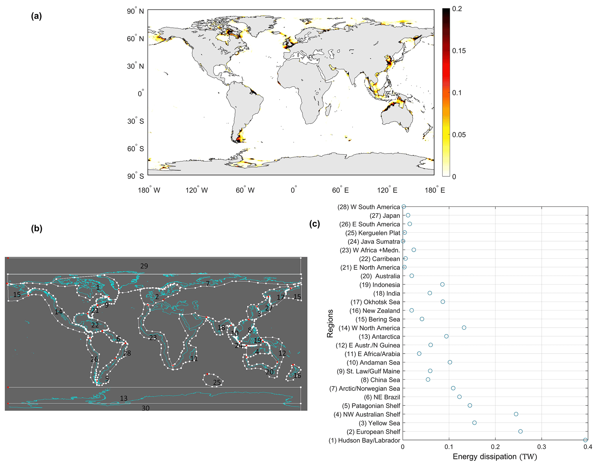
Figure 1Bottom friction energy dissipation in initial GTSMv4.1: (a) global distribution (unit: W m−2); (b) area identification; (c) area-integrated energy dissipation (unit: TW).
It is impractical to estimate the bathymetry and the bottom friction coefficient for all the grid cells because of the limited observations, and it would also be computationally demanding with high memory requirements. To reduce the parameter dimension, we divide the global ocean into 110 subdomains for bathymetry estimation and define the correction factor for each subdomain to adjust the parameters (Wang et al., 2021b). The estimation subdomains for the bottom friction term are located in areas with high dissipation based on Fig. 1c and sufficient coastal observations, as explained in more detail in Sect. 3.
2.3.2 Observation network
Global tide data from the FES2014 dataset and several global or regional tide gauge datasets were collected as observations in the calibration or model validation process.
- –
The FES2014 dataset contains 34 tidal constituents from the FES (finite-element solution) tide model that assimilates altimeter time series and tide gauge data (Carrere et al., 2013; Lyard et al., 2021). FES2014 data have higher accuracy than GTSMv4.1 in the deep ocean when compared with the deep-ocean bottom pressure recorder data (Wang et al., 2021b). Moreover, FES2014 data are distributed on a regular grid and time series can be derived at arbitrary locations globally. Therefore, the dataset is selected to use as observations for the deep ocean to estimate bathymetry correction.
- –
Tide gauge data
- –
The UHSLC (University of Hawaii Sea Level Center) dataset (Caldwell et al., 2010) contains water levels from 500 globally distributed tide gauges. The number of available locations varies in time. Stations in the UHSLC dataset are irregularly distributed, and most of the gauges are in coastal regions. We use the research-quality-controlled dataset, which is considered to be composed of science-ready data.
- –
The CMEMS (Copernicus Marine Environment Monitoring Service) dataset has a collection of in situ tide gauges located in the Arctic Ocean, Baltic Sea, European northwestern shelf seas, Iberian–Biscay–Ireland regional seas, Mediterranean Sea, and Black Sea. All the available data are published after data acquisition, data quality control, product validation, and product distribution. CMEMS data are for the European shelf and are suitable for local bottom friction coefficient estimation.
- –
Arctic tide gauge data have four major constituents. Kowalik and Proshutinsky (1994) described approximate tide stations in the Arctic Ocean and studied the tide performance. Four major tidal constituents (semidiurnal constituents M2 and S2; diurnal constituents K1 and O1) are available. Since only four major tidal constituents cannot fully represent the tide time series for calibration, they are used for the model validation to evaluate the model performance in the frequency domain.
- –
We select the year 2014 for the model analysis because the available tide gauges vary in different years and 2014 has the largest number of stations. Tide analysis is performed with the tide gauge data from the CMEMS and UHSLC dataset for the year 2014 with the TIDEGUI software, a MATLAB implementation of the approach by Schureman (1958), and we visually inspect the tide and surge representations. After the analysis and quality control, we obtained 237 locations in the UHSLC dataset and 297 locations from the CMEMS dataset. In the deep ocean, 4000 time series are generated from the FES2014 dataset to ensure enough observations for estimating bathymetry in the year 2014. These observations are evenly distributed and located in the deep ocean with a depth of more than 200 m.
Even though we obtained three collections of tide gauges, the observations are still quite sparse in some coastal seas. Therefore, we first investigate how to make use of the available data with the consideration of the model performance and parameter sensitivity.
3.1 Model and observation accuracy analysis
The FES2014 dataset is very accurate in the deep ocean (Stammer et al., 2014; Wang et al., 2021b), while along the coast, tide gauge data can be more trustworthy. However, tide gauge data are distributed irregularly. We propose using a combination of the FES2014 dataset and tide gauge data in shallow water. The first step is to analyze the accuracy of the FES2014 dataset and the initial GTSMv4.1 by comparing with the tide gauge data. The root mean square (rms) that describes the difference between model output and observations for tidal components is applied with the formula
Am and Ao are model output and observation amplitudes, ϕm and ϕo are for the phase lag, and ω is the tide frequency. The overbar shows the averaging over one full cycle of the constituent (ωt varying from 0 to 2π) in all locations. We also use the root sum square (RSS) to describe the root square sum of the rms for the listed major tidal constituents. To facilitate comparison, we use the same formulas for RSS and rms as in Stammer et al. (2014).
Table 2 illustrates the root sum square (RSS) and rms of eight major tide components between FES2014 and the initial GTSM with the tide gauge data. The RSS was calculated for all the eight components in all locations. Comparing with the UHSLC dataset globally, FES2014 is more accurate than the GTSM for all of the eight components, generally implying that the FES2014 dataset can provide better tide representation in shallow water than the GTSM. This conclusion is also supported by the comparison with the stations in the Arctic Ocean. Figure 2 shows the spatial distribution of RSS for each location, which shows that with a few exceptions FES2014 is more accurate.
In the European shelf, the GTSM has an RSS of 19.15 cm when comparing with the CMEMS dataset, which is even smaller than the FES2014 dataset with an RSS of 20.42 cm. This also can be observed from the rms of the N2, M2, S2, and K2 constituents. However, from the spatial distribution of RSS for each station shown in Fig. 2c and d, FES2014 performs better in most of the CMEMS locations but provides poor results in a few stations. This results in a larger RSS for FES2014 than the GTSM. A possible reason is that these tide components obtained from FES2014 are calculated by interpolating the gridded FES2014 dataset to the observation locations, resulting in some errors. The GTSM has a higher resolution in the European shelf, contributing to better results in those locations with complex bathymetry. In general, FES2014 outperforms GTSMv4.1 in shallow waters before calibration. It can be used as observations in the parameter estimation application for the GTSM if “real observations”, such as tide gauges, are lacking in some regions.
Table 2RSS and rms of eight major tide components between the FES2014 dataset, initial GTSM, and tide gauge data (unit: cm).
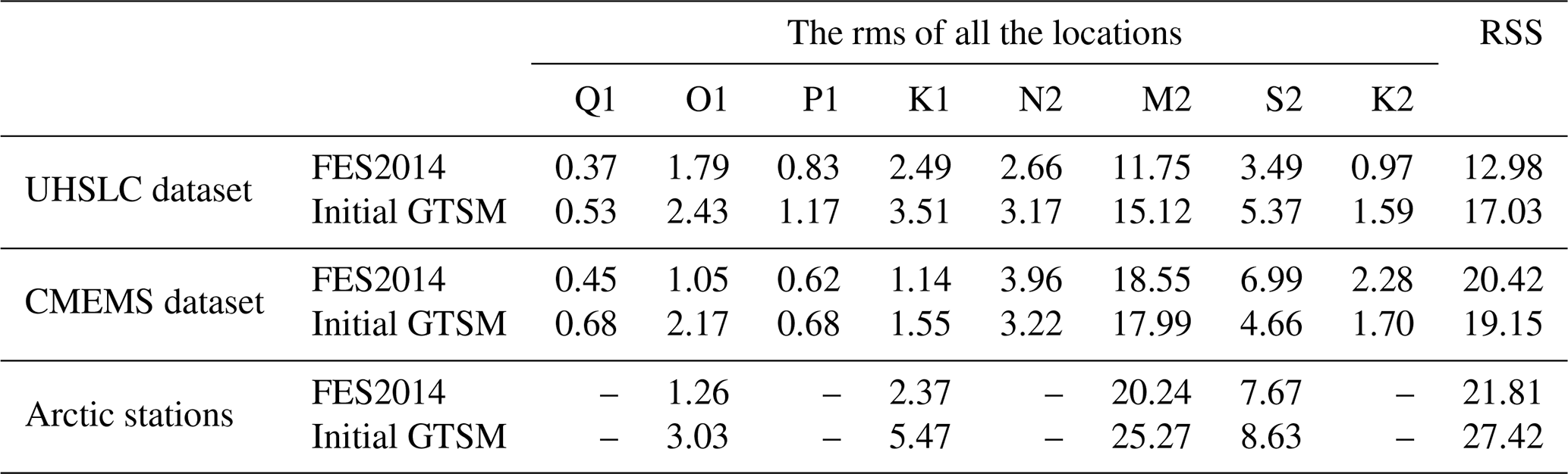
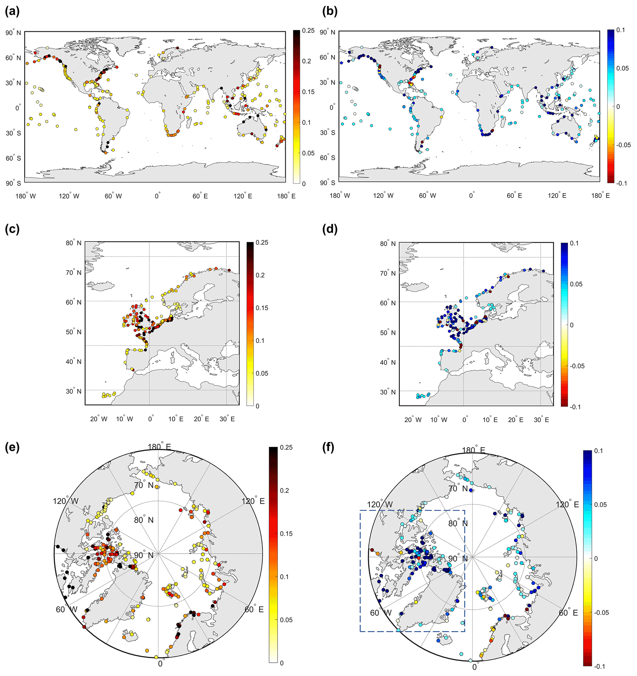
Figure 2Left column: RSS between initial GTSMv4.1 and tide gauge data. Right column: RSS difference between initial GTSMv4.1 and the FES2014 dataset (RSS of GTSM minus RSS of FES2014). Blue shows better performance in FES2014 than the GTSM. (a, b) UHSLC dataset; (c, d) CMEMS dataset; (e, f) Arctic stations (unit: m).
3.2 Subdomains of constant bottom friction coefficient
The bottom friction coefficients in the regions with large tide energy dissipation (see Fig. 1c) have to be estimated. We define multiple subdomains for the European shelf and Hudson Bay–Labrador regions as well as single subdomains for other coastal areas with the consideration of observations, energy dissipation, and seabed topography distributions.
3.2.1 Case region 1: Hudson Bay and Labrador region
The Hudson Bay and Labrador region, at the top of the list in Fig. 1b, generates about 0.39 TW energy dissipation, which is 16.47 % of the global sum. Most of the dissipation is concentrated in the Canadian archipelago, Hudson Bay, Foxe Basin, Hudson Strait, and Ungava Bay (Fig. 3a). We defined three subdomains that firstly separate the Canadian archipelago from the other areas. Secondly, Foxe Basin, Hudson Strait, and Ungava Bay are combined as one subdomain. The last subdomain is for Hudson Bay. Subdomains are shown in the red boxes in Fig. 3a.
The available tide gauge observations are from the Arctic stations but only include four major tidal components. In theory, harmonic tide analysis can be performed for the model output, and it is possible to estimate parameters with the model output of harmonic constants for tidal constituents, but accurate tide analysis needs a time series of a year, which would increase the computational demand. For example, Wang et al. (2021b) reported that a full time series of 1 month is sufficient for an accurate parameter estimation. However, the yearly tide analysis would increase run times by a factor of 12. This is not feasible for us at the moment. Therefore, we choose to use the model output of time series covering 1 month in the estimation process and 1 year for harmonic tide analysis. The Arctic stations can be used for model validation rather than model calibration.
We propose generating observations from the FES2014 dataset to offset the measurements missing in the Hudson Bay. Figure 2e illustrates the RSS (root sum square) of four major tidal constituents between tide gauge data in the Arctic Ocean and the FES2014 dataset. The RSS difference between the GTSM and FES2014 dataset (RSS between the GTSM and tide gauge data – RSS between FES2014 and tide gauge data) varies for each location, and FES2014 has a smaller RSS than the GTSM in most of the locations, especially in the Canadian archipelago regions (Fig. 2f). The RSS of four major tidal constituents for all the locations in the FES2014 dataset is 21.81 cm, while it is 27.82 cm for the GTSM. Errors are typically larger near the coast. Performance of FES2014 at the Arctic stations is better than the GTSM before the calibration. We expect the accuracy of FES in open water to be even better. As a result, 61 equally distributed time series are derived from the FES2014 dataset as observations for the locations in Fig. 3b.
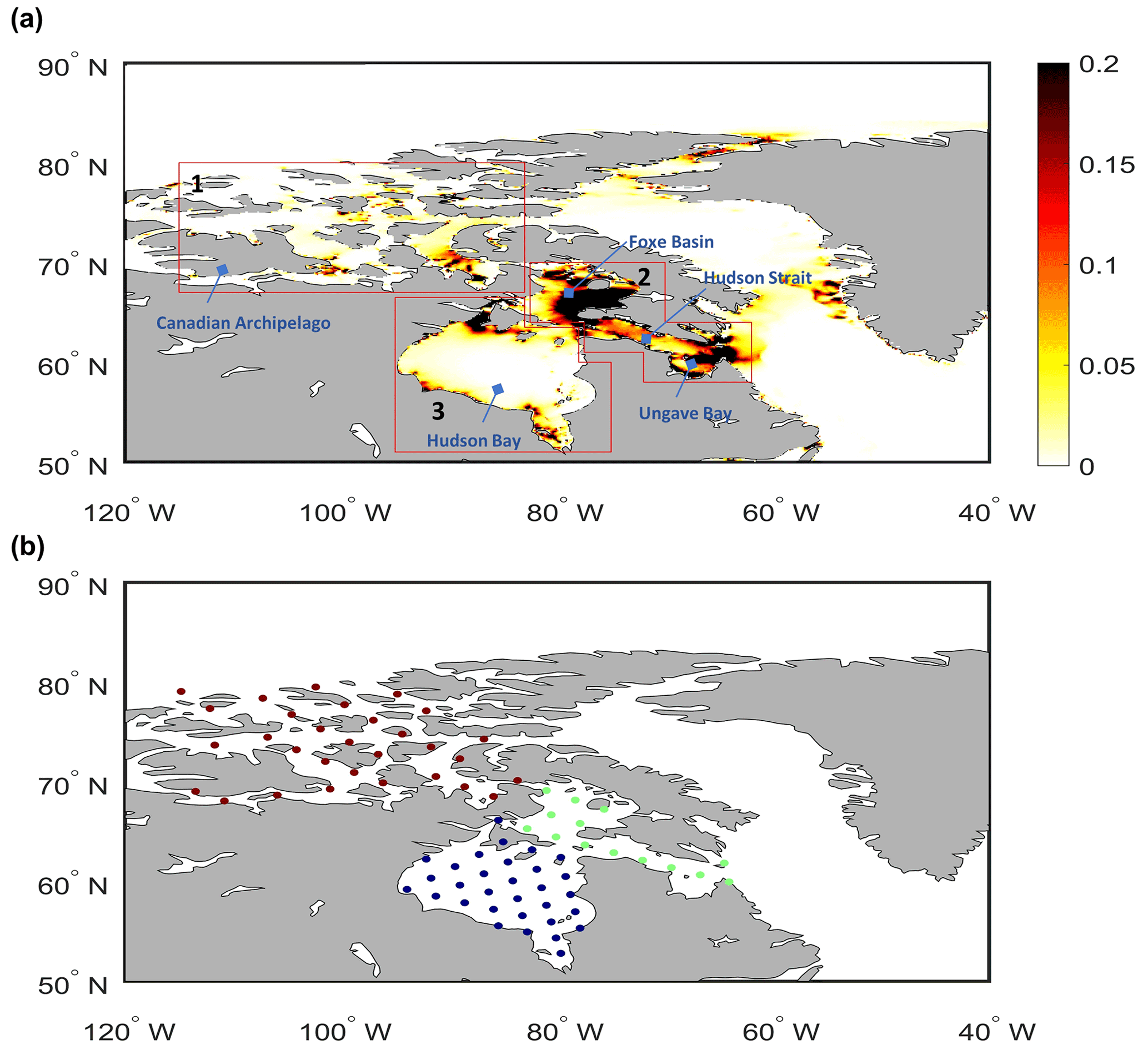
Figure 3(a) Bottom friction energy dissipation per square meter of the Hudson Bay and Labrador in GTSMv4.1 (unit: W m−2) as well as in bottom friction coefficient subdomains (red boxes). (b) FES2014 observation distribution: points with different colors indicate a different subdomain.
3.2.2 Case region 2: European shelf
Bottom friction energy dissipation in the European shelf is about 0.25 TW, which is approximately 10.62 % of the global total value shown in Fig. 4a. Considering the dissipation distribution, we define five subdomains to estimate the bottom friction coefficient. Firstly, we define subdomains for the areas in and outside the North Sea and separate the western and eastern part of the North Sea. Secondly, the region of Scotland, the Faro Islands, and Shetland has mountainous ocean bathymetry, where we expect a higher bottom friction coefficient, is set as a subdomain. Therefore, five subdomains are generated for the European shelf for calibration.
The estimation for the European shelf takes advantage of a large amount of local tide gauge data (Fig. 4b). About 297 tide gauge stations from the CMEMS dataset are available for the year 2014, which will directly be used for parameter estimation. A total of 132 tide gauge data stations in the Mediterranean Sea and Baltic Sea (blue points in Fig. 4b) are removed because they are only weakly connected to the open ocean. The remaining stations are divided into two subsets: 70 locations for calibration (red points in Fig. 4b) and 95 points for validation (green points in Fig. 4b).
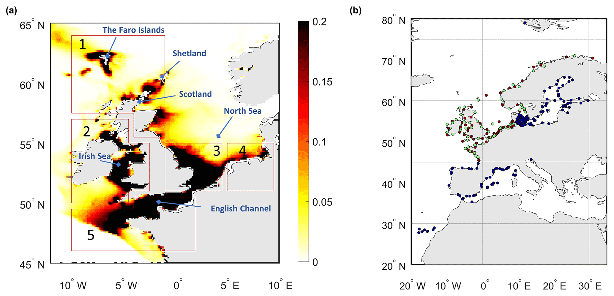
Figure 4(a) Bottom friction energy dissipation per square meter across the European shelf in GTSMv4.1 (unit: W m−2) and bottom friction coefficient subdomains (red boxes). (b) CMEMS observation distribution: points in red are data used for calibration, points in green are used for validation, and points in blue are not used.
3.2.3 Other coastal areas with large energy dissipation
There are many other coastal regions that generate large tide energy dissipation (Fig. 1c), such as the northwest of the Australian shelf and the Yellow Sea. We defined 11 additional subdomains globally. They are in the northwestern Australian shelf, Yellow Sea, Patagonian shelf, Sea of Okhotsk, northeast of Brazil, Arctic–Norwegian Sea, Antarctica, Andaman Sea, China Sea, Bering Sea, and Indonesia. Because of the limited tide gauge availability in shallow water and limited computational resources, it is not feasible to do a detailed subdomain analysis for each of these regions. The detailed subdomain distribution is shown in Sect. 4.
The UHSLC dataset is a collection of global tide gauges, but these measurements are not evenly distributed and lack data in some areas, such as the northwest of Brazil and the Sea of Okhotsk. To make the research on these areas feasible, we propose using more FES2014 data in these regions for estimation and using the UHSLC dataset for validation only. Therefore, additional equally distributed time series (in terms of distance) were generated from FES2014 in locations with bathymetry between 50 and 200 m.
In summary, we defined 110 subdomains for bathymetry and 19 subdomains for bottom friction coefficient estimation (five in the European shelf, three in the Hudson Bay–Labrador region, and 11 for other coastal areas). In total, 4061 time series from the FES2014 dataset and 70 time series from the CMEMS dataset are included in the estimation procedure. The GTSM after the estimation will be validated by comparing with time series from the FES2014 dataset in the deep ocean and tide gauge data from the CMEMS, UHSLC, and Arctic stations.
4.1 Parameter estimation
4.1.1 Experiment design
In the parameter estimation procedure, the GTSM is simulated with tide only because the surge is not sensitive to small random perturbations of the bathymetry (Wang et al., 2021b) but is strongly affected by the meteorological condition. We selected a period of 1 month, September 2014, for the estimation runs. We found that it is sufficient for tide calibration when using high-frequency time series with 10 min sampling (Wang et al., 2021b). In addition, sea ice in the Arctic Ocean is not modeled in the GTSM, but it has seasonal changes to the tides (Bij de Vaate et al., 2021). Performing the experiment in September can minimize the impact of sea ice on the model because of no ice coverage in September. To ensure that the 1-month estimation is realistic, meteorological and long-period signals have to be reduced as much as possible. We made model runs without atmospheric forcing and removed the SA and SSA tidal potential to avoid seasonal changes to the time series because long-term constituents show large variation between years. These constituents were also removed from the FES2014 and tide gauge series to keep the comparison consistent.
The time step for the model output and observation is 10 min, leading to a time number in a 1-month simulation equal to Nt=4321. The number of observation locations from FES2014 and CMEMS together is Ns=4131. Moreover, parameters are corrected for the 110 bathymetry subdomains and 19 bottom friction subdomains. In this case, the data size refers to observations, and model output for all the ensembles (perturbed parameters) in the estimated process is about 17.3 GB. With the implementation of POD-based time pattern order reduction, a truncation size of 200 represents the model output and observations in a smaller subspace of time patterns. The memory requirement is reduced by a factor of 22 after the POD application.
Several constraints are defined in the optimization process to ensure that the adjusted parameters are realistic. The uncertainty for the bathymetry correction factor is set to 5 % and for the bottom friction coefficient to 20 %. Bathymetry uncertainty is defined as 5 % from the knowledge that only a fraction of the ocean seabed has been surveyed, and the remaining errors are significant (Tozer et al., 2019). We empirically defined the uncertainty by investigating its varying range. Initially, each parameter is perturbed one by one with the uncertainty value to obtain the model output for each ensemble. The same values are also used for a weak constraint, adding to the cost function as the background term. It defines the difference between the initial and adjusted parameters. The background term can avoid changes to the parameter far away from the initial values that only achieve an insignificant improvement. In addition, hard constraints are also defined as the upper and lower boundary for the parameters. They are twice the uncertainty with the value of [−10 %, 10 %] for bathymetry and [−40 %, 40 %] for the bottom friction coefficient. Finally, there is a transition zone between each subdomain to avoid a sudden change in the correction factor from one subdomain to another. The correction factor in the transition zone is generated by automatic linear interpolation.
4.1.2 Parameter estimation results
Before the performance of parameter estimation, the sensitivities of each subdomain for bottom friction and bathymetry are analyzed in Fig. 5. Bathymetry and bottom friction have comparable sensitivities (Fig. 5a–b). The sensitivity values of bathymetry vary between −0.06 and 0.02 (Fig. 5a). The sensitivity of the bottom friction coefficient changes between −0.01 and 0.05 (Fig. 5b), with the largest value up to approximately 0.05 in the northwest of the Australian shelf. As we discussed in the Introduction, bottom friction impacts the model performance not only in the local shallow waters but also in the nearby deep ocean. It can be observed in Fig. 5c–f when perturbing the bottom friction in the subdomains of European shelf and Hudson Bay. Standard deviation (SD) is large in the nearby oceans around the perturbing subdomain and smaller when the location is far away, and the largest SD values are located around the coastline (Fig. 5d). Bottom friction in the Hudson Bay subdomain has a larger effect on the surrounding deep oceans (Fig. 5c) than the European shelf (Fig. 5e). It is consistent with the largest tide energy dissipation being in Hudson Bay.

Figure 5(a) Sensitivity for bathymetry. Sensitivity is the relative changes in the cost function, describing the difference between the model output and the observations when perturbing each parameter; (b) sensitivity for bottom friction coefficient; (c–f) SD between initial model output and model output with perturbed bottom friction coefficient (unit: m). Panels (c) and (d) illustrate the SD with the perturbation of subdomain 5 of the European shelf in Fig. 4a; panels (e) and (f) show the perturbation of subdomain 3 of Hudson Bay in Fig. 3a. Panels (c) and (e) show the 4061 evenly distributed locations, which are the same locations as the FES2014 dataset used in the parameter estimation. (d) The SD at the tide gauge locations around the EU. (f) The observation points from the FES2014 dataset in detail in the Hudson Bay.
Figure 6a illustrates the cost function changes for each iteration in these four outer loops. The first 130 iterations in each loop perturb parameters one by one; parameters are iteratively updated after that until reaching the stop criteria. Optimized parameters in this outer loop will be used as the initial parameters to start the next loop. The estimation experiment was performed with 200 cores and nine cluster nodes running for about 16 d, with a total cost of approximately 76 800 CPU core hours.
The cost function in the experiment started from the value of 1.96×10⁷. It is sharply reduced in the first outer loop to the value of 6.40×10⁶, resulting in a reduction by 67.3 %. The decrease in the cost function in the second to fourth outer loop is slight and converged in the fourth loop with the value of 5.58×10⁶. Finally, the cost function is reduced by 71.5 %. The relative changes in bathymetry and the bottom friction coefficient are shown in Fig. 6b and c. After the estimation, the total tide energy dissipation is reasonable with a value of 3.77 TW.
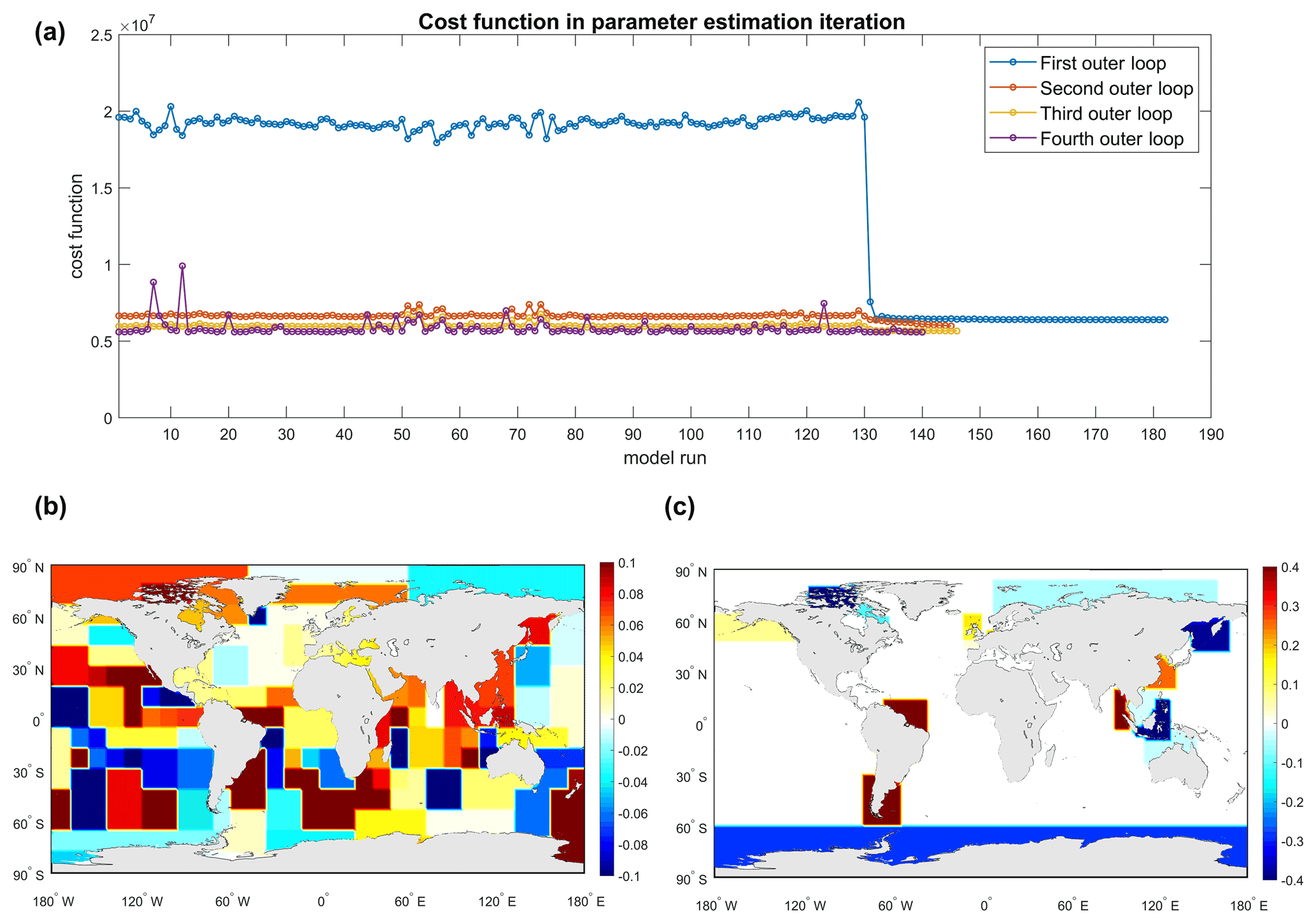
Figure 6(a) Value of the cost function for each model run during the estimation; (b) relative changes in bathymetry (bathymetry correction factor) after the estimation; (c) relative changes in bottom friction coefficient (bottom friction coefficient correction factor) after estimation.
The average spatial SD between model output and observations in September 2014 is summarized in Table 3. Compared with the FES2014 dataset, the spatial average SD is sharply reduced by 52.4 % after the estimation from 5.19 to 2.47 cm. The total reduction is significant in the first outer loop and slight in the second to fourth outer loops. It is observed that in the Arctic Ocean, the initial SD with the value of 11.03 cm is larger than other regions. It is expected because we added more observation points in the Hudson Bay and Labrador region. This area is shallower with large tide amplitudes, resulting in larger SD than other regions. Therefore, the comparison here includes the observations located in the deep ocean and shallow water together.
The outer-loop iterations provide more improvement in the Arctic Ocean than in other regions. A possible explanation is that parameter estimation impacts areas with large disagreement against observations most because they still have room to improve, and nonlinear effects become more likely. In Europe, the GTSM shows significant improvement compared to CMEMS tide gauge data for calibration and validation, which are reduced by 36.1 % and 30.5 %, respectively. The difference between model and UHSLC data is significantly reduced in the first outer loop and finally decreased by 24.3 %. This decline is smaller than that in CMEMS data for two reasons. First, the UHSLC data are not included in the estimation process. Secondly, many shallow waters where the UHSLC tide gauges located are not defined for the bottom friction coefficient estimation. For example, only two tide gauges are available in the Arctic Ocean, and no stations are in the Hudson Bay area.
The spatial distribution of the SD for the estimated GTSM and the SD difference between the initial and estimated model in September 2014 are shown in Fig. 7. The SD between the estimated model and FES2014 dataset is larger in shallow water, such as the northwest of the Australian shelf and Hudson Bay–Labrador, than in the deep ocean (Fig. 7a). It can be observed that the estimated model is significantly improved with the SD reduced by about 2 cm for most of the regions in the deep ocean (Fig. 7b). Using more time series from the FES2014 dataset in the Hudson Bay and Labrador plays a role in the estimation process since the model is in excellent agreement with the FES2014 dataset for most observation points. Several locations in the middle area of Hudson Bay are a bit worse.
Compared with the CMEMS dataset in Fig. 7g and h, the parameter estimation brings a large improvement to the European shelf, with the SD reduced from 17.60 to 11.25 cm. This demonstrates that the direct use of tide gauge data in the estimation can improve model performance in shallow waters. Figure 7c and d also illustrate that the SD between the model and the UHSLC dataset is decreased by a small amount. Figure 7e and f report the comparison with the UHSLC dataset for the Australian shelf, where we defined several subdomains for bottom friction estimation. Even though the subdomains here are not as detailed as in the Hudson Bay and the European shelf, the SD is also greatly reduced after the calibration in most of the tide gauges.
Table 3Average SD between the GTSM and observations in September 2014 (unit: cm). Numbers with bold font show the smallest SD value among the four iterations.
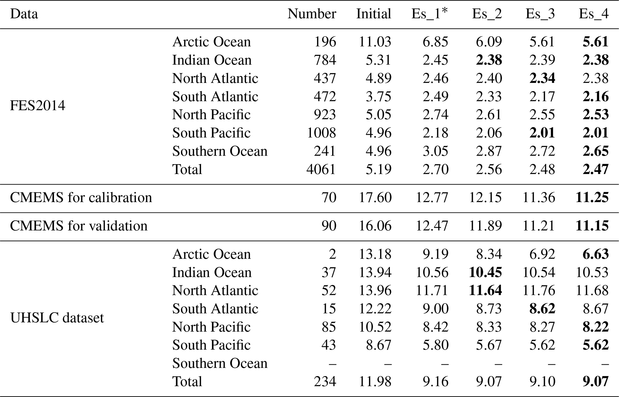
* Es_1, Es_2, Es_3, and Es_4 indicate the estimated GTSM in the first, second, third, and fourth outer loop.
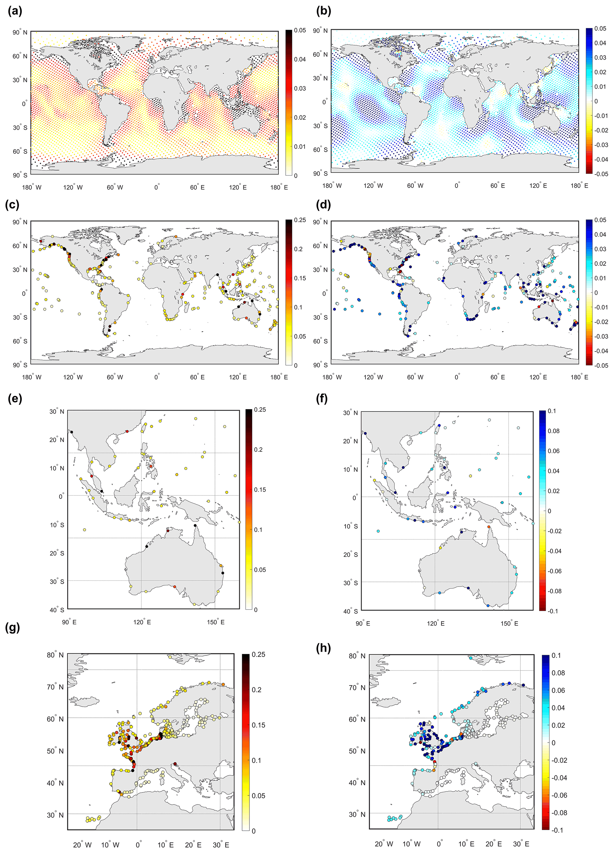
Figure 7Left column: spatial distribution of the SD of the estimated GTSM. Right column: the SD difference between the initial model and estimated model from 1 to 30 September 2014. SD difference is defined as the RMSE of the initial model minus SD of estimated GTSMv4.1. Blue in the right column shows improvements in the estimated model (unit: m). The observation datasets used to compare with GTSMv4.1: (a, b) FES2014 dataset; (c, d) UHSLC dataset; (e, f) UHSLC dataset around the Australian shelf; (g, h) CMEMS dataset.
4.2 Model validation in the year 2014
To evaluate the model forecast ability, we firstly validate the time series water level (tide and surge) from the GTSM in the year 2014 with the comparison of FES2014 and tide gauge data, following by the major tidal component analysis.
4.2.1 Monthly time series comparison
Figure 8 shows the average SD between the GTSM and FES2014 time series for each month of 2014 in seven ocean regions (Fig. 8a–g). Most of the observations are located in the deep ocean. Compared to the initial GTSM, results in the calibration period and the other months of 2014 have reached similar accuracy, implying that the estimation is not over-fitting the observations we used. The SD in the Arctic Ocean is larger than other regions, which coincides with the results in Table 3.
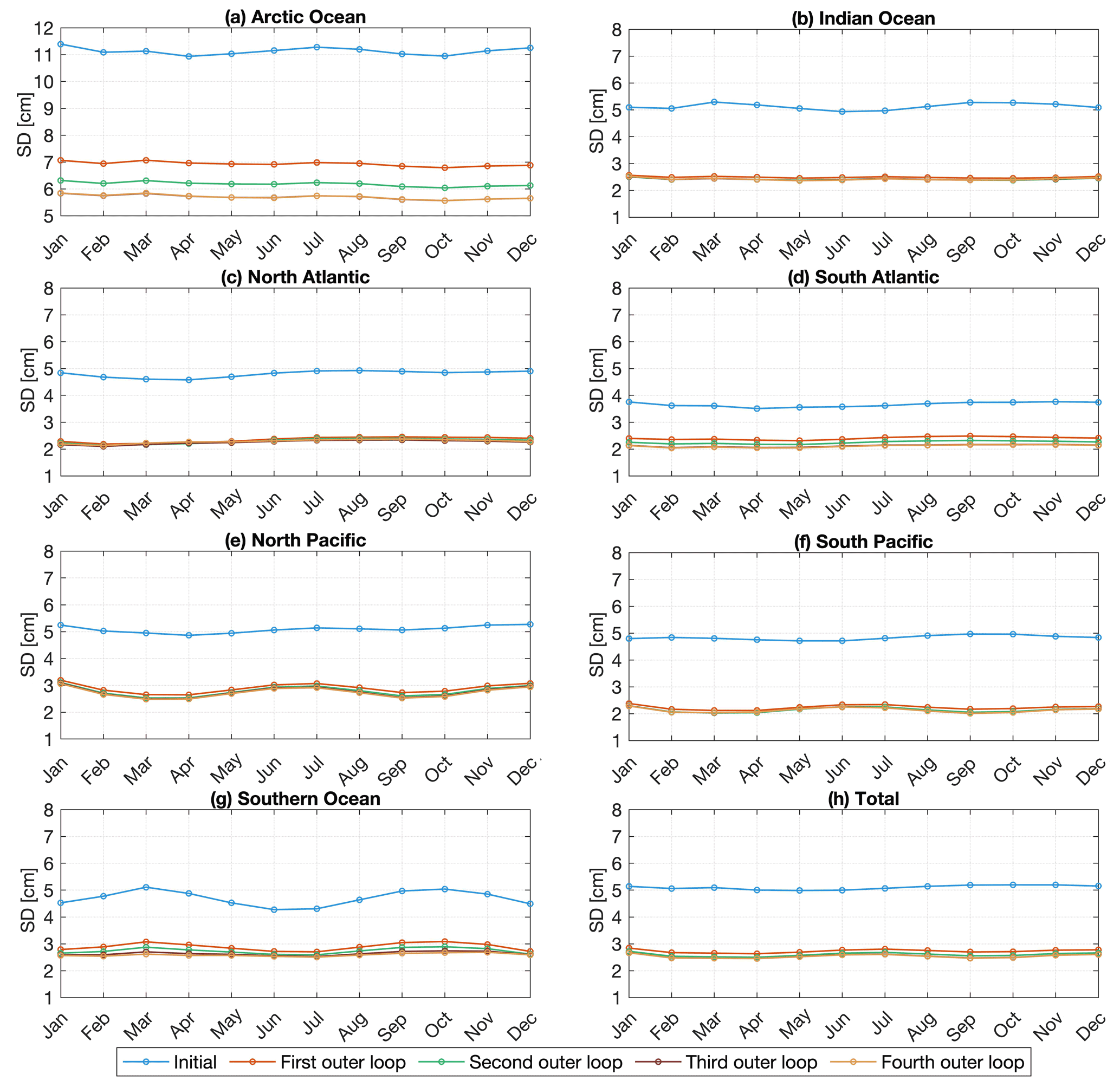
Figure 8Regionally averaged SD between the GTSMv4.1 and FES2014 dataset in 2014 for tide simulation (unit: cm).
Model-derived tide representation is compared with the CMEMS and UHSLC tide gauge data in Fig. 9. CMEMS data in Fig. 9a include all the stations for calibration and validation. The average spatial SD for the year 2014 in the initial model is 16.7 cm. After the first outer-loop estimation, a large reduction is achieved to a value of 12.38 cm. Accuracy is further improved due to the outer-loop iteration. Finally, the SD is reduced to 66.5 %. The direct use of CMEMS tide gauge data for calibration of the bottom friction coefficient effectively reduces the model error that came from parameter uncertainty and results in high-accuracy tide representation in shallow waters.
In this study, the UHSLC tide gauge dataset is only used for validation (Fig. 9b). It shows that the calibration also has better agreement in shallow waters outside Europe. But because many of the stations from the UHSLC dataset are not in the estimation subdomains we defined, the improvement is limited.
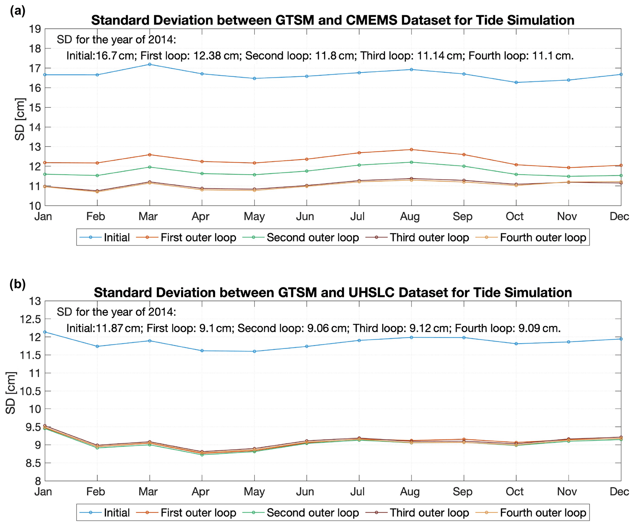
Figure 9Spatially averaged SD between GTSMv4.1 and tide gauges in 2014 for tide simulation (unit: cm); (a) CMEMS dataset; (b) UHSLC dataset.
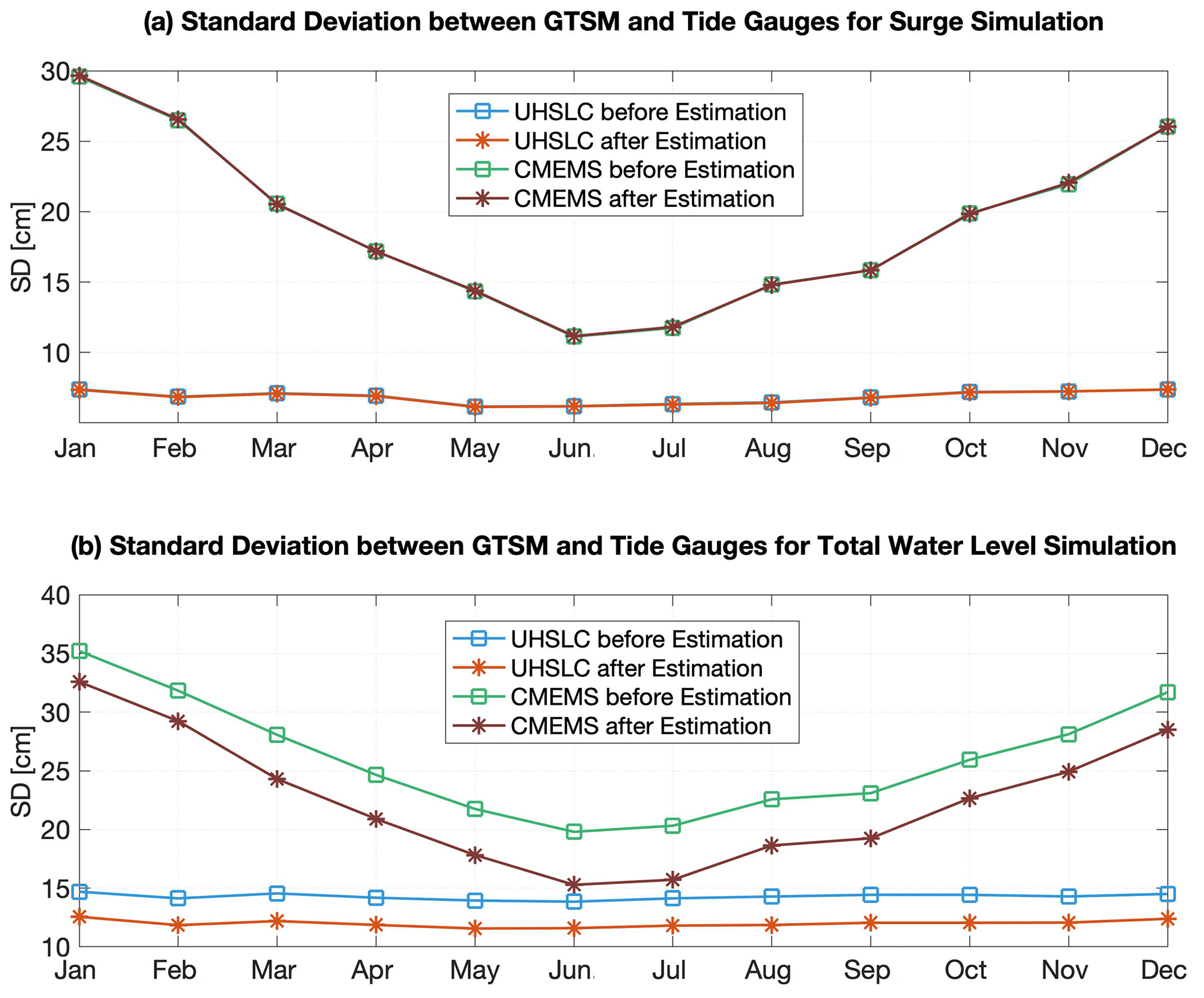
Figure 10(a) Spatially averaged SD between GTSMv4.1 and tide gauges for surge simulation in 2014; (b) spatially averaged SD between GTSMv4.1 and tide gauges for total water level simulation in 2014 (unit: cm). CMEMS data include 165 points (70 points are used in the calibration process and 95 points are for validation).
The standard deviation of surge simulation before and after the estimation shows minor difference in Fig. 10. It is consistent with findings in our previous research estimating bathymetry for the GTSM (Wang et al., 2021b). The errors are generally larger in the areas with stronger tide in shallow waters. This makes the absolute value of the SD very dependent on the tide gauges that are used. In the UHSLC dataset, the locations are spread over the planet. The CMEMS dataset focuses on the European shelf with stronger winds in winter.
In general, these comparisons show that surge is not sensitive to the bathymetry and bottom friction but strongly affected by the wind and air pressure conditions. This conclusion is also supported by Chu et al. (2019) regarding the sensitivity of surge in the East China Sea (their Fig. 13). In our study, even though surge simulation keeps the same accuracy after the estimation, the water level forecast accuracy is improved because of the improvement of tide representations, which is significantly demonstrated in Fig. 10b. Therefore, the bottom friction and bathymetry estimation improves the model-derived water level forecast ability in the coastal areas. Moreover, we expect to conduct further research on the impact on the surge and the nonlinear interaction between surge and tide with higher resolution in more complex estuarine and river regions in the future.
4.2.2 Tidal constituent analysis
To further study the global tides, we performed a 1-year harmonic analysis for 2014 on the model-derived tide representation before and after the estimation and compared the major eight components with observations.
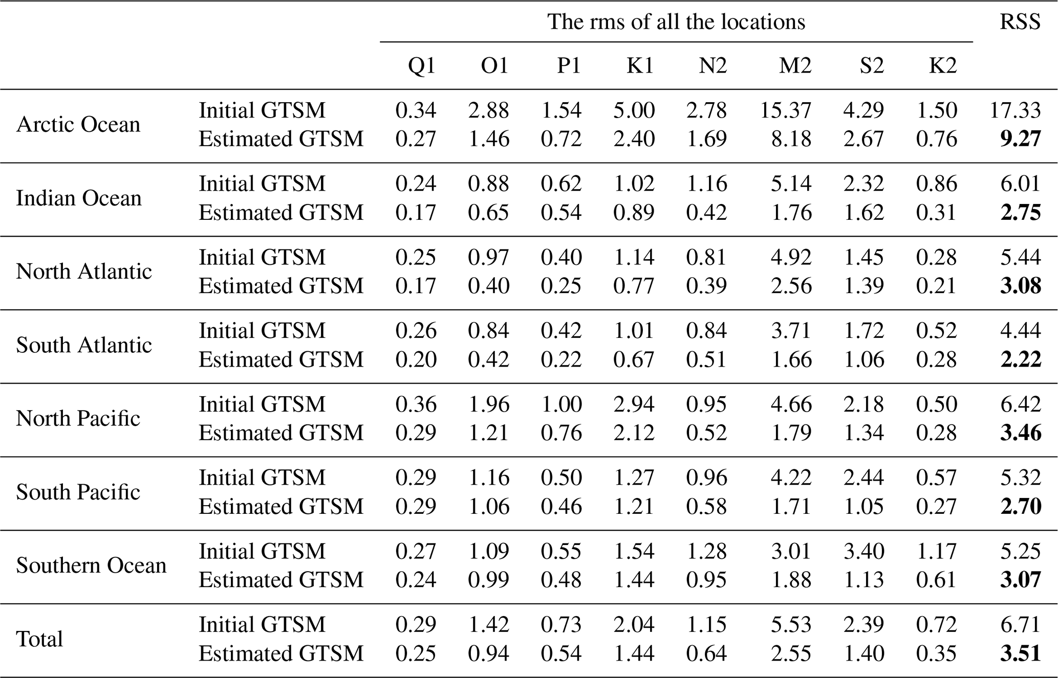
Table 4 compares the tidal analysis results of the GTSM and FES2014 before and after the estimation. The estimated GTSM has higher accuracy for all eight major tide components, with the RSS reduced by 47.7 %. The largest rms is in the M2 tidal constituent. The rms of tidal constituents M2, S2, K1, and O1 in the Arctic Ocean is much larger than other regions before and after the estimation. This can also be observed from the spatial distribution of the amplitude and phase of the M2 tide component in Fig. 11. We observed large tide amplitudes in shallow waters, such as in the Hudson Bay, European shelf, and the Australian shelf, and small amplitudes in the deep ocean (Fig. 11a). It results in large amplitude differences between the GTSM and observations in the Hudson Bay and Labrador regions (Fig. 11b), as well as a higher SD for the Arctic Ocean. After the estimation, amplitude and phase differences are reduced in most regions (Fig. 11c, f). The largest amplitude differences in Fig. 11c are still in the areas around the Hudson Bay, Foxe Basin, Hudson Strait, and Ungava Bay, even though the difference is significantly reduced compared with the initial model.
Table 4RSS and rms of eight major tide components between the GTSM and FES2014 dataset (unit: cm). Numbers with bold font show the smaller value of RSS when comparing the initial GTSM with the estimated GTSM.
In Table 5, we compare the tide components with the deep-ocean bottom pressure recorder (BPR) data in the deep ocean to assess the model performance with other tide models described by Stammer et al. (2014). BPR data are available from the Supplement of Ray (2013). Compared with non-assimilative tide models, the initial GTSM has an rms of 4.77 cm in the M2 component that outperforms the purely hydrodynamic tide models described in Table 12 of Stammer et al. (2014). In the estimation process, we select the FES2014 dataset as observations for the deep ocean with a smaller RSS than the initial GTSM. The FES2014 dataset is also the successor of FES2012. For example, RSS of FES2014 is 0.58 cm, while it is 1.12 cm in the FES2012 dataset (Table 3 in Stammer et al., 2014). After the estimation, the RSS of the GTSM is reduced to 2.83 cm. Even though it is still not as accurate as FES2014 or other assimilative tide models (Table 3 in Stammer et al., 2014), it is excellent compared to non-assimilative models. In addition, the GTSM, like non-assimilative models, can be used in scenario studies, such as studying climate change.
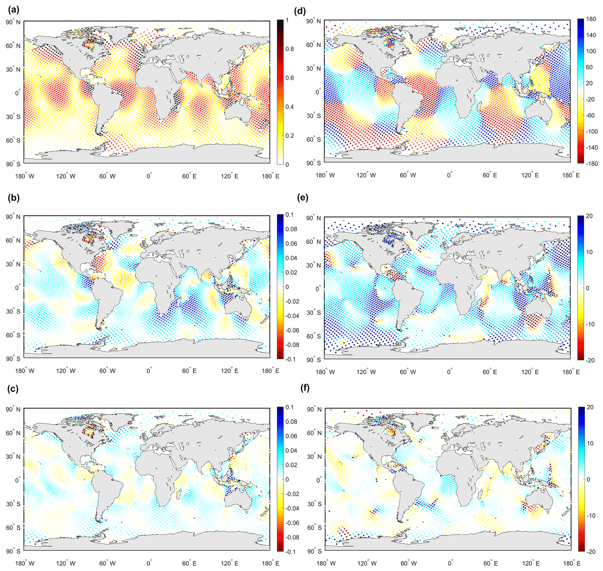
Figure 11Spatial distribution of M2 amplitudes and phases from GTSMv4.1 and the FES2014 dataset. (a) Amplitudes of M2 for the FES2014 dataset; (b, c) amplitude differences between FES2014 and the initial GTSM and between FES2014 and the estimated model, respectively (unit: m). (d) Phases of M2 for the FES2014 dataset; (e, f) phase differences between FES2014 and the initial GTSM and between FES2014 and the estimated model, respectively (unit: ∘).
Table 5RSS and rms of eight major tide components between GTSM and deep-ocean bottom pressure recorder (BPR) data1 (unit: cm).
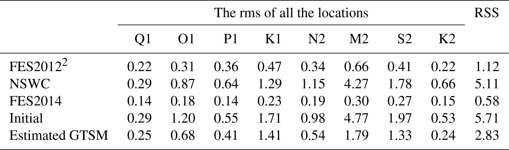
1 BPR data are available from the Supplement of Ray (2013). 2 Results of NSWC and FES2012 are from Stammer et al. (2014) Table 3.
Table 6RSS and rms of eight major tide components between the GTSM and tide gauges (CMEMS, UHSLC, and Arctic stations) (unit: cm).
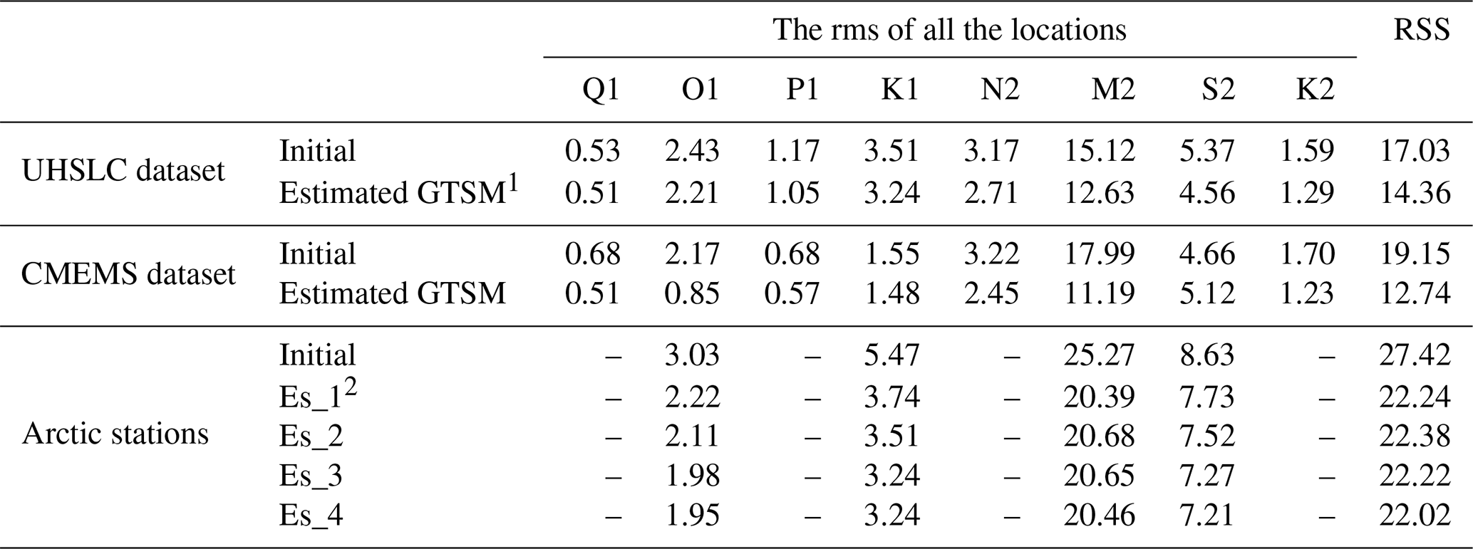
1 Estimated GTSM is the estimated GTSM in the fourth outer loop. 2 Es_1, Es_2, Es_3, and Es_4 indicate the estimated GTSM in the first, second, third, and fourth outer loop.

Figure 12RSS of four major tide components between the Arctic station and initial GTSMv4.1 (a) as well as estimated GTSMv4.1 (b). (c) RSS difference between the initial model and estimated model (RSS of the initial model minus RSS of the estimated model). (d) RSS of the estimated model minus RSS between FES2014 and Arctic stations (unit: m). Blue shows better performance in the estimated GTSM than the initial model (c) or FES2014 dataset (d).
In shallow water, we summarized the rms of major tide components with the comparison of tide gauge data in Table 6. After the estimation, the RSS of the GTSM is reduced by 16 % of the initial GTSM from 17.03 to 14.36 cm. The error is still larger than in the FES2014 dataset with the value of 12.98 cm in Table 2.
Compared with the CMEMS dataset (all locations in the calibration and validation subsets), the RSS of all eight components is reduced from 19.15 to 12.74 cm. After the estimation, model errors have the largest reduction in the European shelf compared to other regions. These results also demonstrate that directly assimilating tide gauge data can significantly improve the accuracy of tide representation in models.
In the Arctic Ocean, we analyze the four major tide components from Arctic stations and the GTSM. As a special area that has different performance in the outer iterations of the estimation process than other regions, we report results with the comparison of Arctic stations in four outer loops in Table 6. The rms is reduced after the first outer loop, especially for the M2 component, resulting in the value of 22.24 cm. It is close to the accuracy of the FES2014 shown in Table 2. However, the total accuracy in the second to fourth outer loop is not further improved. The M2 constituent becomes a bit worse, but other tide frequencies are improved. This is contrasted with the results in Table 3 and Fig. 8a for the comparison with FES2014 data in Arctic Ocean. An explanation is that most of the Arctic stations are located in the Canadian archipelago, not the Hudson Bay. In addition, there are still observation errors in FES2014 even though FES2014 provides higher accuracy than the initial GTSM. Estimation leads the results closer to the FES2014 but not constantly closer to the Arctic stations because of the observation error in FES2014 and the uncertainties with the Arctic stations. The spatial distribution of RSS for each station is illustrated in Fig. 12. We can observe that error of the GTSM after estimation is smaller than before (Fig. 12a–c). However, the estimated GTSM does not surpass the accuracy of the FES2014 dataset (Fig. 12d), which we also did not expect. Therefore, it is concluded that the observation error significantly influences the estimation accuracy. Moreover, stations in Norway seem to get worse (Fig. 12c), which is inconsistent with CMEMS data.
In summary, model assessments from the time and frequency fields demonstrate that the parameter estimation of bathymetry and the bottom friction coefficient can significantly improve the tide representation in the deep ocean and shallow waters. The GTSM benefits from estimating the bottom friction coefficient, especially in the Hudson Bay–Labrador and the European shelf. The combined use of FES2014 and tide gauge data offsets the scarce observations in shallow water and improves model skills after the parameter estimation. The direct use of tide gauge data provides excellent agreement between the observation and model output after the estimation. The estimated GTSM can provide high-accuracy total water level forecast in shallow waters, which is useful to assess the risk from coastal flooding, study the sea level rise and the interaction between tide and surge.
This paper presents a study about the joint estimation of bathymetry and the bottom friction coefficient for the Global Tide and Surge Model (GTSM), which effectively improves the global tide representation, especially in shallow waters. Bathymetry is the main parameter affecting model performance at the worldwide scale (Wang et al., 2021b), and the bottom friction term influences the tide representation in areas with significant tide energy dissipation (shallow–coastal areas). The FES2014 dataset, with higher accuracy than the initial GTSM in the deep ocean, is used for calibration in this paper. It plays a vital role in correcting the bathymetry factor in the ocean domain we defined. To ensure that the estimation for the bottom friction coefficient is feasible, we propose a combination of FES2014 and tide gauge data for the estimation of bottom friction in shallower coastal waters. Applying this parameter estimation significantly improves the tide representation of the GTSM almost everywhere around the globe.
The Hudson Bay–Labrador Sea and European shelf are the regions with the largest tide energy dissipation. The bottom friction coefficient in the European shelf is optimized with the tide gauge data from the CMEMS dataset. This results in the largest improvements of tide accuracy for shallow waters. We refined the observation locations from the FES2014 dataset in the Hudson Bay and Labrador Sea. This approach is based on the condition that data from Arctic stations only have four major tide components that cannot be used for calibration, and FES2014 has higher accuracy than the initial GTSM when comparing against these stations. After estimation the accuracy of the GTSM is close to that of FES here. Moreover, some other coastal areas with large energy dissipation are estimated by including more observations located at depths 50–200 m from the FES2014 dataset because the numbered UHSLC tide gauges are too few to be used for calibration directly in many regions. After calibration, the GTSM has smaller disagreement than the initial model but is not as accurate as the FES2014 dataset when comparing with the UHSLC dataset. The RSS of eight tide components between FES2014 and UHSLC tide gauge data is 12.98 cm, which is smaller than the estimated GTSM with the value of 14.36 cm. However, the purpose of the calibration of the GTSM is different from that of FES2014. The GTSM is used as a strong constraint. A consequence is that this dramatically reduces the number of degrees of freedom for the assimilation, leading in general to larger differences with the observations. It is likely that the calibrated GTSM produces less accurate tides but can be used for a wider range of applications. These remarks discuss the assimilation aspect only, but other factors, such as the resolution, quality of the input data, and the physics included in the model, also contribute to the accuracy of the final result. Finally, the amount and quality of the assimilated observations also influence the accuracy. FES2014 assimilates a large number of observations from both remote sensing and in situ studies, achieving very high accuracy in deep waters, which is why we have selected it as a data source for our calibration.
In summary, the accuracy of the GTSM is significantly improved with the combined parameter estimation of bathymetry and the bottom friction coefficient. Tide representation in shallow waters benefits from the optimization of the bottom friction coefficient, contributing to a more accurate water level forecast when including wind and air pressure conditions for surge simulation. Accurate parameter estimation for global tide models needs sufficient observations and a proper determination of parameter subdomains. Direct utilization of tide gauge data provides the most significant reduction of model error. For some areas such as the Hudson Bay, with insufficient tide gauge measurements, the use of other data with higher accuracy than the model can also improve the model performance to a certain extent. The 1-year model validation demonstrates that the estimated GTSM can provide long-term high-accuracy tide forecasts. Thanks to the efforts of communities like GLOSS, UHSLC, CMEMS, EMODnet, and GESLA, more and more tide gauge data are becoming available. However, the spatial scales in shallow coastal waters are much smaller than in deep water, so the number of available tide gauges is not yet sufficient for calibration of tide models at the moment. Satellite altimetry has the potential to add much more information about tides in shallow waters. However, compound tides, overtides, and tide–surge interaction will make this more complicated than in deeper waters.
To further reduce tide errors using the presented parameter estimation technique, some major obstacles remain: (1) when we include satellite altimetry data, especially in shallow water, in the estimation process, the accuracy of harmonic tidal analysis for the satellite altimetry has to be assessed, which would require complex preprocessing. (2) The influence of sea ice on the tide is currently not yet included in the model. However, the seasonal modulation from sea ice can affect the model performance (Kagan and Sofina, 2010; Müller et al., 2014) because sea ice exerts additional frictional stress on the surface. In our parameter estimation experiment, we observed that in the Canadian archipelago, higher bottom friction coefficients are estimated. This is probably caused by a lack of dissipation by sea ice. However, the estimated bottom friction coefficients do not result in good agreement with the seasonal dynamics. A possible solution is to include the sea ice modeling in the GTSM, and the sea ice coefficient will also become an uncertain source to estimate. This will also require measurements that properly represent modulation of the tides over the seasons. Preliminary products of this type are starting to appear (Bij de Vaate et al., 2021).
The Delft3D Flexible Mesh software can be obtained from Deltares upon request (https://oss.deltares.nl/web/delft3dfm, Open Source Community, 2022). The OpenDA software can be obtained from https://github.com/OpenDA-Association/OpenDA (OpenDA Association, 2022). The FES2014 dataset is acquired from https://www.aviso.altimetry.fr/en/data/products/auxiliary-products/global-tide-fes/description-fes2014.html (AVISO, 2022). Research-quality data from UHSLC are made available through the University of Hawaii Sea Level Center with the link ftp://ftp.soest.hawaii.edu/uhslc/rqds (last access: 31 May 2022) and https://doi.org/10.7289/V5V40S7W (Caldwell et al., 2015). The CMEMS data can be obtained from https://marine.copernicus.eu/ (last access: 31 May 2022) and https://doi.org/10.13155/43494 (Copernicus Marine In Situ Tac Data Management Team, 2021). Bathymetry data are available from https://www.gebco.net/data_and_products/gridded_bathymetry_data/gebco_2019/gebco_2019_info.html (GEBCO, 2019) and https://www.emodnet-bathymetry.eu/data-products (EMODnet, 2022).
XW and MV conceived the study and designed the parameter estimation scheme. JV prepared the GTSMv4.1. XW performed the estimation experiments and carried out the data analysis. MV, HXL, and JV provided useful comments on the paper. XW prepared the paper with contributions from MV and all other co-authors.
The contact author has declared that neither they nor their co-authors have any competing interests.
Publisher's note: Copernicus Publications remains neutral with regard to jurisdictional claims in published maps and institutional affiliations.
This work was carried out on the Dutch national e-infrastructure with the support of SURF.
This research has been supported by the State Scholarship Fund from the China Scholarship Council (grant no. 201703170275).
This paper was edited by Joanne Williams and reviewed by William Pringle and one anonymous referee.
Arbic, B. K., Mitrovica, J. X., MacAyeal, D. R., and Milne, G. A.: On the factors behind large Labrador Sea tides during the last glacial cycle and the potential implications for Heinrich events, Paleoceanography, 23, PA3211, https://doi.org/10.1029/2007PA001573, 2008. a
Arbic, B. K., Wallcraft, A. J., and Metzger, E. J.: Concurrent simulation of the eddying general circulation and tides in a global ocean model, Ocean Model., 32, 175–187, https://doi.org/10.1016/j.ocemod.2010.01.007, 2010. a
AVISO: Global Tide – FES2014, AVISO [data set], https://www.aviso.altimetry.fr/en/data/products/auxiliary-products/global-tide-fes/description-fes2014.html, last access: 31 May 2022. a
Bij de Vaate, I., Vasulkar, A. N., Slobbe, D. C., and Verlaan, M.: The Influence of Arctic Landfast Ice on Seasonal Modulation of the M2 Tide, J. Geophys. Res.-Ocean., 126, e2020JC016630, https://doi.org/10.1029/2020JC016630, 2021. a, b
Blakely, C. P., Ling, G., Pringle, W. J., Contreras, M. T., Wirasaet, D., Westerink, J. J., Moghimi, S., Seroka, G., Shi, L., Myers, E., and Owensby, M.: Dissipation and Bathymetric Sensitivities in an Unstructured Mesh Global Tidal Model, Earth Space Sci. Open Arch., 127, e2021JC018178, https://doi.org/10.1002/essoar.10509993.1, 2022. a
Cai, H., Toffolon, M., Savenije, H. H. G., Yang, Q., and Garel, E.: Frictional interactions between tidal constituents in tide-dominated estuaries, Ocean Sci., 14, 769–782, https://doi.org/10.5194/os-14-769-2018, 2018. a
Caldwell, P. C., Merrifield, M. A., and Thompson, P. R.: Sea level measured by tide gauges from global oceans as part of the Joint Archive for Sea Level (JASL) since 1846, NOAA National Centers for Environmental Information, NOAA National Centers for Environmental Information [data set], https://doi.org/10.7289/v5v40s7w, 2010. a
Caldwell, P. C., Merrifield, M. A., and Thompson, P. R.: Sea level measured by tide gauges from global oceans — the Joint Archive for Sea Level holdings (NCEI Accession 0019568), Version 5.5, NOAA National Centers for Environmental Information [data set], https://doi.org/10.7289/V5V40S7W, 2015. a
Carrere, L., Lyard, F., Cancet, M., Guillot, A., and Roblou, L.: FES 2012: A New Global Tidal Model Taking Advantage of Nearly 20 Years of Altimetry, in: 20 Years of Progress in Radar Altimatry, edited by: Ouwehand, L., ESA Special Publication, 710, p. 13, https://ui.adsabs.harvard.edu/abs/2013ESASP.710E..13C (last access: 31 May 2022), 2013. a
Cheng, Y. and Andersen, O. B.: Towards further improving DTU global ocean tide model in shallow waters and Polar Seas, OSTST, Poster in: Proceedings of the Ocean Surface Topography Science Team (OSTST) Meeting, Miami, FL, USA, 23–27 October, 2017. a
Chu, D., Zhang, J., Wu, Y., Jiao, X., and Qian, S.: Sensitivities of modelling storm surge to bottom friction, wind drag coefficient, and meteorological product in the East China Sea, Estuarine, Coast. Shelf Sci., 231, 106460, https://doi.org/10.1016/j.ecss.2019.106460, 2019. a
Colebrook, C. F., White, C. M., and Taylor, G. I.: Experiments with fluid friction in roughened pipes, P. R. Soc. Lond. A Mat., 161, 367–381, https://doi.org/10.1098/rspa.1937.0150, 1937. a
Copernicus Marine In Situ Tac Data Management Team: Product User Manual for multiparameter Copernicus In Situ TAC (PUM), Copernicus [data set], https://doi.org/10.13155/43494, 2021. a
Edwards, C. A., Moore, A. M., Hoteit, I., and Cornuelle, B. D.: Regional Ocean Data Assimilation, Ann. Rev. Mar. Sci., 7, 21–42, https://doi.org/10.1146/annurev-marine-010814-015821, 2015. a
Egbert, G. D. and Erofeeva, S. Y.: Efficient Inverse Modeling of Barotropic Ocean Tides, J. Atmos. Ocean. Technol., 19, 183–204, https://doi.org/10.1175/1520-0426(2002)019<0183:EIMOBO>2.0.CO;2, 2002. a
Egbert, G. D. and Ray, R. D.: Estimates of M2 tidal energy dissipation from TOPEX/Poseidon altimeter data, J. Geophys. Res.-Ocean., 106, 22475–22502, https://doi.org/10.1029/2000JC000699, 2001. a, b, c, d, e
EMODnet: Data products, EMODnet [data set], https://www.emodnet-bathymetry.eu/data-products, last access: 31 May 2022. a
GEBCO: GEBCO_2019 Grid, GEBCO [data set], https://www.gebco.net/data_and_products/gridded_bathymetry_data/gebco_2019/gebco_2019_info.html (last access: 31 May 2022), 2019. a, b
Hallegatte, S., Green, C., Nicholls, R., and Corfee-Morlot, J.: Future flood losses in major coastal cities, Nat. Clim. Change, 802–806, https://doi.org/10.1038/nclimate1979, 2013. a
Hart-Davis, M. G., Piccioni, G., Dettmering, D., Schwatke, C., Passaro, M., and Seitz, F.: EOT20: a global ocean tide model from multi-mission satellite altimetry, Earth Syst. Sci. Data, 13, 3869–3884, https://doi.org/10.5194/essd-13-3869-2021, 2021. a
Heemink, A., Mouthaan, E., Roest, M., Vollebregt, E., Robaczewska, K., and Verlaan, M.: Inverse 3D shallow water flow modelling of the continental shelf, Cont. Shelf Res., 22, 465–484, https://doi.org/10.1016/S0278-4343(01)00071-1, 2002. a, b
Kagan, B. and Sofina, E.: Ice-induced seasonal variability of tidal constants in the Arctic Ocean, Cont. Shelf Res., 30, 643–647, https://doi.org/doi.org/10.1016/j.csr.2009.05.010, 2010. a
Kowalik, Z. and Proshutinsky, A. Y.: The Arctic ocean tides, Washington DC American Geophysical Union Geophysical Monograph Series, 85, 137–158, https://doi.org/10.1029/GM085p0137, 1994. a, b
Kron, W.: Coasts: the high-risk areas of the world, Nat. Hazards, 66, 1363–1382, https://doi.org/10.1007/s11069-012-0215-4, 2012. a
Kuhlmann, J., Dobslaw, H., and Thomas, M.: Improved modeling of sea level patterns by incorporating self-attraction and loading, J. Geophys. Res.-Ocean., 116, C11036, https://doi.org/10.1029/2011JC007399, 2011. a
Lyard, F. H., Allain, D. J., Cancet, M., Carrère, L., and Picot, N.: FES2014 global ocean tide atlas: design and performance, Ocean Sci., 17, 615–649, https://doi.org/10.5194/os-17-615-2021, 2021. a, b, c
Manning, R.: On the Flow of Water in Open Channels and Pipes, Transactions Institute of Civil Engineers of Ireland, Dublin, 1891. a, b
Mayo, T., Butler, T., Dson, C. N., and Hoteit, I.: Data assimilation within the Advanced Circulation (ADCIRC) modeling framework for the estimation of Manning's friction coefficient, Ocean Model., 76, 43–58, https://doi.org/10.1016/j.ocemod.2014.01.001, 2014. a, b
McGranahan, G., Balk, D., and Anderson, B.: The rising tide: assessing the risks of climate change and human settlements in low elevation coastal zones, Environ. Urban., 19, 17–37, https://doi.org/10.1177/0956247807076960, 2007. a
Muis, S., Verlaan, M., Nicholls, R. J., Brown, S., Hinkel, J., Lincke, D., Vafeidis, A. T., Scussolini, P., Winsemius, H. C., and Ward, P. J.: A comparison of two global datasets of extreme sea levels and resulting flood exposure, Earth's Future, 5, 379–392, https://doi.org/10.1002/2016EF000430, 2017. a
Muis, S., Apecechea, M. I., Dullaart, J., de Lima Rego, J., Madsen, K. S., Su, J., Yan, K., and Verlaan, M.: A High-Resolution Global Dataset of Extreme Sea Levels, Tides, and Storm Surges, Including Future Projections, Front. Mar. Sci., 7, 263, https://doi.org/10.3389/fmars.2020.00263, 2020. a
Munk, W. and Wunsch, C.: Abyssal recipes II: energetics of tidal and wind mixing, Deep-Sea Res. Pt. I, 45, 1977–2010, https://doi.org/10.1016/S0967-0637(98)00070-3, 1998. a
Müller, M., Cherniawsky, J. Y., Foreman, M. G. G., and von Storch, J.-S.: Global M2 internal tide and its seasonal variability from high resolution ocean circulation and tide modeling, Geophys. Res. Lett., 39, L19607, https://doi.org/10.1029/2012GL053320, 2012. a
Müller, M., Cherniawsky, J. Y., Foreman, M. G. G., and von Storch, J.-S.: Seasonal variation of the M2 tide, Ocean Dynam., 64, 159–177, https://doi.org/10.1007/s10236-013-0679-0, 2014. a
Navon, I.: Practical and theoretical aspects of adjoint parameter estimation and identifiability in meteorology and oceanography, Dynam. Atmos. Ocean., 27, 55–79, https://doi.org/10.1016/S0377-0265(97)00032-8, 1998. a
Nycander, J.: Generation of internal waves in the deep ocean by tides, J. Geophys. Res.-Ocean., 110, C10028, https://doi.org/10.1029/2004JC002487, 2005. a, b
OpenDA Association: OpenDA, GitHub [code], https://github.com/OpenDA-Association/OpenDA, last access: 31 May 2022. a
OpenDA User Documentation: https://www.openda.org/docu/openda_2.4/doc/OpenDA_documentation.pdf, last access: 10 June 2016. a
Open Source Community: Delft3D FM, https://oss.deltares.nl/web/delft3dfm, last access: 31 May 2022. a
Oppenheimer, M., Glavovic, B., Hinkel, J., Wal, R. V. D., Magnan, A., Abd-EIGawad, A., Cai, R., Cifuentes-Jara, M., DeConto, R., Ghosh, T., Hay, J., Isla, F., Marzeion, B., Meyssignac, B., and Sebesvári, Z.: Sea Level Rise and Implications for Low Lying Islands, Coasts and Communities, in: IPCC Special Report on the Ocean and Cryosphere in Climate, Cambridge University Press, Cambridge, 321–446 https://doi.org/10.1017/9781009157964.006, 2019. a
Pringle, W. J., Wirasaet, D., Roberts, K. J., and Westerink, J. J.: Global storm tide modeling with ADCIRC v55: unstructured mesh design and performance, Geosci. Model Dev., 14, 1125–1145, https://doi.org/10.5194/gmd-14-1125-2021, 2021. a
Provost, C. and Lyard, F.: Energetics of the M2 barotropic ocean tides: an estimate of bottom friction dissipation from a hydrodynamic model, Prog. Oceanogr., 40, 37–52, https://doi.org/10.1016/S0079-6611(97)00022-0, 1997. a
Pugh, D. and Woodworth, P.: Sea-Level Science: Understanding Tides, Surges, Tsunamis and Mean Sea-Level Changes, Cambridge University Press, https://doi.org/10.1017/CBO9781139235778, 2014. a
Ralston, M. L. and Jennrich, R. I.: Dud, A Derivative-Free Algorithm for Nonlinear Least Squares, Technometrics, 20, 7–14, https://doi.org/10.1080/00401706.1978.10489610, 1978. a
Ray, R. D.: Precise comparisons of bottom-pressure and altimetric ocean tides, J. Geophys. Res.-Ocean, 118, 4570–4584, https://doi.org/10.1002/jgrc.20336, 2013. a, b, c
Schureman, P.: Manual of Harmonic Analysis and Prediction of Tides, US Department of Commerce, Coast and Geodetic Survey, https://doi.org/10.25607/OBP-155, 1958. a
Siripatana, A., Mayo, T., Knio, O., Dawson, C., Maître, O. L., and Hoteit, I.: Ensemble Kalman filter inference of spatially-varying Manning's n coefficients in the coastal ocean, J. Hydrol., 562, 664–684, https://doi.org/10.1016/j.jhydrol.2018.05.021, 2018. a
Slivinski, L., Pratt, L., Rypina, I., Orescanin, M., Raubenheimer, B., MacMahan, J., and Elgar, S.: Assimilating Lagrangian data for parameter estimation in a multiple-inlet system, Ocean Model., 113, 131–144, https://doi.org/10.1016/j.ocemod.2017.04.001, 2017. a
Stammer, D., Ray, R. D., Andersen, O. B., Arbic, B. K., Bosch, W., Carrère, L., Cheng, Y., Chinn, D. S., Dushaw, B. D., Egbert, G. D., Erofeeva, S. Y., Fok, H. S., Green, J. A. M., Griffiths, S., King, M. A., Lapin, V., Lemoine, F. G., Luthcke, S. B., Lyard, F., Morison, J., Müller, M., Padman, L., Richman, J. G., Shriver, J. F., Shum, C. K., Taguchi, E., and Yi, Y.: Accuracy assessment of global barotropic ocean tide models, Rev. Geophys., 52, 243–282, https://doi.org/10.1002/2014RG000450, 2014. a, b, c, d, e, f, g, h, i, j
Taguchi, E., Stammer, D., and Zahel, W.: Inferring deep ocean tidal energy dissipation from the global high-resolution data-assimilative HAMTIDE model, J. Geophys. Res.-Ocean., 119, 4573–4592, https://doi.org/10.1002/2013JC009766, 2013. a
Tozer, B., Sandwell, D. T., Smith, W. H. F., Olson, C., Beale, J. R., and Wessel, P.: Global Bathymetry and Topography at 15 Arc Sec: SRTM15+, Earth Space Sci., 6, 1847–1864, https://doi.org/10.1029/2019EA000658, 2019. a
Trémolet, Y.: Incremental 4D-Var convergence study, Tellus A, 59, 706–718, https://doi.org/10.1111/j.1600-0870.2007.00271.x, 2007. a
Ullman, D. S. and Wilson, R. E.: Model parameter estimation from data assimilation modeling: Temporal and spatial variability of the bottom drag coefficient, J. Geophys. Res.-Ocean., 103, 5531–5549, https://doi.org/10.1029/97JC03178, 1998. a
Verlaan, M., De Kleermaeker, S., and Buckman, L.: GLOSSIS: Global storm surge forecasting and information system, Auckland, New Zealand, Engineers Australia and IPENZ, 229–234, https://doi.org/10.3316/informit.703696922952912, 2015. a, b
Vitousek, S., Barnard, P., Fletcher, C., Frazer, N., Erikson, L., and Storlazzi, C.: Doubling of coastal flooding frequency within decades due to sea-level rise, Sci. Rep., 7, 1–9, https://doi.org/10.1038/s41598-017-01362-7, 2017. a
Wahl, T., Haigh, I. D., Nicholls, R. J., Arns, A., Dangendorf, S., Hinkel, J., and Slangen, A. B. A.: Understanding extreme sea levels for broad-scale coastal impact and adaptation analysis, Nat. Commun., 8, 16075, https://doi.org/10.1038/ncomms16075, 2017. a
Wang, D., Zhang, J., and Wang, Y. P.: Estimation of Bottom Friction Coefficient in Multi-Constituent Tidal Models Using the Adjoint Method: Temporal Variations and Spatial Distributions, J. Geophys. Res.-Ocean., 126, e2020JC016949, https://doi.org/10.1029/2020JC016949, 2021a. a
Wang, X., Verlaan, M., Apecechea, M. I., and Lin, H. X.: Computation-Efficient Parameter Estimation for a High-Resolution Global Tide and Surge Model, J. Geophys. Res.-Ocean, 126, e2020JC016917, https://doi.org/10.1029/2020JC016917, 2021b. a, b, c, d, e, f, g, h, i, j, k, l, m, n, o, p, q
Wang, X., Verlaan, M., Apecechea, M. I., and Lin, H. X.: Parameter estimation for a global tide and surge model with a memory-efficient order reduction approach, Ocean Model., 173, 102011, https://doi.org/10.1016/j.ocemod.2022.102011, 2022. a, b
Ward, P., Jongman, B., Salamon, P., Simpson, A., Bates, P., de Groeve, T., Muis, S., Coughlan, E., Rudari, R., Trigg, M., and Winsemius, H.: Usefulness and limitations of global flood risk models, Nat. Clim. Change, 5, 712–715, https://doi.org/10.1038/nclimate2742, 2015. a
Wölfl, A.-C., Snaith, H., Amirebrahimi, S., Devey, C. W., Dorschel, B., Ferrini, V., Huvenne, V. A. I., Jakobsson, M., Jencks, J., Johnston, G., Lamarche, G., Mayer, L., Millar, D., Pedersen, T. H., Picard, K., Reitz, A., Schmitt, T., Visbeck, M., Weatherall, P., and Wigley, R.: Seafloor Mapping – The Challenge of a Truly Global Ocean Bathymetry, Front. Mar. Sci., 6, 283, https://doi.org/10.3389/fmars.2019.00283, 2019. a
Zaron, E. D.: Topographic and frictional controls on tides in the Sea of Okhotsk, Ocean Model., 117, 1–11, https://doi.org/10.1016/j.ocemod.2017.06.011, 2017. a
Zhang, S., Liu, Z., Zhang, X., Wu, X., Han, G., Zhao, Y., Yu, X., Liu, C., Liu, Y., Wu, S., Lu, F., Li, M., and Deng, X.: Coupled data assimilation and parameter estimation in coupled ocean–atmosphere models: a review, Clim. Dynam., 54, 5127–5144, https://doi.org/10.1007/s00382-020-05275-6, 2020. a
Zijl, F., Verlaan, M., and Gerritsen, H.: Improved water-level forecasting for the Northwest European Shelf and North Sea through direct modelling of tide, surge and non-linear interaction, Ocean Dynam., 63, 823–847, https://doi.org/10.1007/s10236-013-0624-2, 2013. a, b, c