Quasi-steady circulation regimes in the Baltic Sea

Circulation plays an essential role in the creation of physical and biogeochemical fluxes in the Baltic Sea. The main aim of the work was to study the quasi-steady circulation patterns under prevailing forcing conditions.

A total of 6 months of continuous vertical profiling and fixed-point measurements of currents, two month-long underwater glider surveys, and numerical modeling were applied in the central Baltic Sea. The vertical structure of currents was strongly linked to the location of the two pycnoclines: the seasonal thermocline and the halocline. The vertical movements of pycnoclines and velocity shear maxima were synchronous. The quasi-steady circulation patterns were in geostrophic balance and highly persistent. The persistent patterns included circulation features such as upwelling, downwelling, and boundary currents, as well as a sub-halocline gravity current. The patterns had a prevailing zonal scale of 5–60 km as well as considerably higher magnitude and different direction than the long-term mean circulation pattern.

A northward (southward) geostrophic boundary current in the upper layer was observed along the eastern coast of the central Baltic in the case of southwesterly (northerly) wind. The geostrophic current at the boundary was often a consequence of wind-driven, across-shore advection.

The sub-halocline quasi-permanent gravity current with a width of 10–30 km from the Gotland Deep to the north over the narrow sill separating the Fårö Deep and Nothern Deep was detected in the simulation, and it was confirmed by an Argo float trajectory. According to the simulation, a strong flow, mostly to the north, with a zonal scale of 5 km occurred at the sill. This current is an important deeper limb of the overturning circulation of the Baltic Sea. The current was stronger with northerly winds and restricted by the southwesterly winds.

The circulation regime had an annual cycle due to seasonality in the forcing. The boundary current was stronger and more frequent northward during the winter period. The sub-halocline current towards the north was strongest in March–May and weakest in November–December.

1 Introduction

Current structure is an important player in the physical and biogeochemical fluxes in ocean. The semi-enclosed, shallow, brackish Baltic Sea has a strong but variable vertical stratification characterized by two pycnoclines: the permanent halocline and the seasonal thermocline (Leppäranta and Myrberg, 2009). A three-layer structure occurs in summer and consists of a warm and less saline upper mixed layer, a cold and saltier intermediate layer, and the warmest and saltiest deep layer. The water column is mixed up to the permanent halocline at 60–80 m depth, and cold intermediate water forms during winters. Stratification through the two pycnoclines impedes vertical mixing, and transport of substances between the layers is limited. The role of tides is marginal in the Baltic Sea. Lateral flows play an important role in distributing the water properties.

Water-mass circulation of the Baltic Sea is determined by the saline water inflow from the North Sea and freshwater input from the catchment area. The interaction of the fresher and saltier waters forms the Baltic haline conveyor belt (Döös et al., 2004). The belt consists of saltier water transport and signal propagation in the deep layer towards the northeastern end of the Baltic (Liblik et al., 2018; Väli et al., 2013), upward salt flux through vertical mixing and transport (Reissmann et al., 2009), and outflow of the mix of riverine and saltier water in the upper layer (Jakobsen et al., 2010). The conveyor determines salinity, stratification, and other important characteristics for the ecosystem.

The largest basin in the sea, the Baltic Proper (Fig. 1a), is a source for the deep waters of the Gulf of Riga, Gulf of Finland, and Gulf of Bothnia. Permanent oxygen depletion has expanded in recent decades in the Baltic Sea, forming one of the largest dead zones in the global ocean (e.g., Carstensen et al., 2014). Only major Baltic inflows (Matthäus and Franck, 1992; Mohrholz, 2018) ventilate the deep layers of the southern and central Baltic Proper (Holtermann et al., 2017) but increase hypoxia in the northern Baltic Proper and Gulf of Finland due to transport of former anoxic–hypoxic eastern Gotland Basin water and stronger stratification (Liblik et al., 2018).

Figure 1 (a) Map of the Baltic Sea and model domain. Shown are the locations of the open boundary of the model domain at the Kattegat (bold black line), Landsort, and Gothenburg sea level stations, as well as the Baltic Sea rivers used in the model (black dots) and study area (blue box). (b) Close-up of the study area. Locations of ADCP and Valeport moorings, CTD measurements, glider section, the center of the cell of ERA5 wind data, and zonal section along the latitude of the ADCP location in the northern Baltic Proper (white dashed line) are presented. Gotland Deep (GD), Fårö Deep (FD), and Nothern Deep (ND) are also shown. The white line marks the section in Fig. 14a, and the red line indicates the time series calculation range for Fig. 14b and c. (c) Close view of the moorings and CTD measurement locations, glider section, and local topography. Dots on land (b–c) illustrate the model grid.

The basin-scale pattern of the long-term mean circulation in the Baltic Proper is cyclonic as demonstrated by several modeling studies (Hinrichsen et al., 2018; Jedrasik et al., 2008; Jędrasik and Kowalewski, 2019; Meier, 2007; Placke et al., 2018). The mean circulation is to the north along the eastern coast of the Baltic Proper and to the south along the eastern and western coast of Gotland Island (Meier, 2007; Placke et al., 2018). The turning area for this basin-wide cyclonic circulation cell in the north is between 59 and 59.5^∘ N (Meier, 2007). The zonal center of the cyclonic flow in the eastern Gotland Basin is in the Gotland Deep (Placke et al., 2018). The cyclonic structure exists from the bottom to the surface (Placke et al., 2018), although the lateral structure and magnitude of the flow vary among different models (Placke et al., 2018). It is important to note that all previously mentioned descriptors of the long-term mean flow rely on numerical simulations and lack support from observations. However, a consistent northward low-frequency current along the eastern slope of the Gotland Deep at 204 m depth has been reported (Hagen and Feistel, 2004). Placke et al. (2018) compared simulated currents with these measurements. All model simulations showed a mean meridional northward current velocity in the range of 0–1 cm s⁻¹ (actually, three models out of four had values of 0.0–0.1 cm s⁻¹), while the measurements gave a mean northward velocity of 3 cm s⁻¹ (Hagen and Feistel, 2004). Thus, the long-term mean flow to the north in the deep layer was much stronger than the simulated mean current.

Temporal variability of currents in the Baltic Sea is very high as a reaction to atmospheric forcing. Nearshore Eulerian current observations (Sokolov and Chubarenko, 2012) and drifter experiments (Golenko et al., 2017; Krayushkin et al., 2019) conducted in the southern Baltic Proper showed a strong correlation between wind and surface currents. Current velocity spectra in the Baltic include seiches and tides with different periods from 11 to 31 h and inertial motions with a period of about 14 h (Jönsson et al., 2008; Lilover et al., 2011; Suhhova et al., 2018).

The vertical current structure through the thermocline and halocline has not been rigorously studied through in situ observations in the Baltic Proper. Moreover, despite considerable effort to reveal the spatial, long-term mean circulation patterns based on the simulations, not much has been done to study temporal developments of currents on synoptic (mesoscale) and seasonal timescales in the Baltic Proper. In the present work, we address this shortage of knowledge.

Permanent circulation systems, such as boundary currents or subtropical gyres, are key processes that determine transport in the open ocean (e.g., Macdonald, 1998). Although there are no permanent currents in the Baltic Sea, we hypothesize that under stable wind forcing and stratification conditions, a steady circulation regime prevails on the timescale of days to weeks and has a much greater magnitude than the mean current structures. These quasi-steady circulation features could be related to the downwelling and upwelling processes or appear as a boundary current or a gravity current under the halocline.

Following a description of the methods used, we present an analysis of (1) the boundary current under variable wind forcing and stratification, (2) quasi-permanent circulation patterns, and (3) the sub-halocline current. The analysis of observational and simulation results is followed by discussion and conclusions.

2 Data and methods

2.1 Observations and data products

A bottom-mounted current profiler (ADCP – acoustic Doppler current profiler, 300 kHz; Teledyne RDI) and model 106 current meter (Valeport Ltd) (hereinafter referred to as Valeport) were deployed at the end of February 2020 to the west of Saaremaa Island (Fig. 1b and c). Valeport was mounted at 5 m depth, while the sea bottom depth in its location ($\mathrm{58}{}^{\circ }{\mathrm{27.4}}^{\prime }$ N, $\mathrm{21}{}^{\circ }{\mathrm{44.4}}^{\prime }$ E) was 41 m. The sea depth in the ADCP location ($\mathrm{58}{}^{\circ }{\mathrm{27.3}}^{\prime }$ N, $\mathrm{21}{}^{\circ }{\mathrm{34.6}}^{\prime }$ E) was 71 m, and velocities were measured with a vertical depth interval of 2 m in the depth range of 10–68 m. Current velocity profiles were recorded as an average of 1 h. The quality of the current velocity data was checked following the procedure developed by Book et al. (2007). Valeport recorded current velocity with 10 min intervals. A Sea-Bird SBE 16plus V2 conductivity–temperature–depth (CTD) SEACAT recorder was deployed together with the ADCP, but it hung 4 m above the sea bottom, i.e., at a depth of 67 m. SBE 16plus sensors were calibrated by the manufacturer before the deployment.

Repeated CTD profiles on board R/V Salme were collected using an OS320 CTD probe (Idronaut S.r.l.) in the northern Baltic Proper (see Fig. 1b and c) from 30 January to 4 August 2020.

Argo float deployment was arranged by the Finnish Meteorological Institute (Siiriä et al., 2019) from 15 August 2013 to 15 August 2014, and the trajectory data were derived from the Argo-based deep displacement dataset (Ollitrault and Rannou, 2013). The dataset was downloaded on 15 March 2021 from https://www.seanoe.org/data/00360/47077/ (last access: 15 March 2021).

In 2020, two glider missions were conducted in the northern Baltic Proper. The Slocum G2 Glider collected oceanographic data along the E–W-oriented 27 km long section (Fig. 1b and c). The easternmost point of the glider track was approximately 7 km off the shoreline, and the section was located at the sloping bottom where sea depth gradually deepened westward from 40 to 90 m. The first mission was carried out from 28 February to 22 March 2020 and the second one from 4 August to 2 September 2020. Both ascending and descending profiles were recorded, and altogether over 8000 profiles were gathered. The glider moved at a horizontal speed of 0.33±0.08 m s⁻¹. On average, a profile took 8.0±0.9 min to complete an 80–90 m deep profile, and the average distance between the profiles near the surface was 301±46 m. Both the sampling time and the distance were decreased by half in the shallow part of the section.

Preliminary glider data processing included standard quality control (impossible date and location test, range tests for the sensors; practically no incorrect data were detected) and accounting for the response time of the sensors and the thermal lag. First, a linear time shift was applied to temperature and conductivity considering the misalignment with pressure. Temperature was re-aligned by 1.4 s and conductivity by 0.9 s for the mission conducted in the spring and by 1.6 and 1.1 s for the mission in the summer. The parameters were chosen by comparing consecutive profiles focusing on the depth range around the greatest gradient. It was assumed that successive profiles correspond to the same water mass. We followed Mensah et al. (2009) to remove the thermal lag effect and found optimal coefficients for the temperature error amplitude, α , and time constant, t_c, by comparing consecutive temperature–salinity profiles. Satisfying results were obtained in the case of α=0.0025 and t_c=10 s for the earlier mission and α=0.055 and t_c=12 s for the following one. The profiles were averaged on a 0.5 dbar vertical grid after processing the raw data.

Sea surface temperature was derived from the Copernicus Marine Service product SST_BAL_SST_L4_REP_OBSERVATIONS_010_016 with a horizontal resolution of $\mathrm{0.02}{}^{\circ }\times \mathrm{0.02}{}^{\circ }$. The mean difference between the product and in situ data sources was in the range of −0.12 to −0.21 ^∘C and root mean square error from 0.43 to 0.88 ^∘C, depending on the data sources, according to the quality information document (https://catalogue.marine.copernicus.eu/documents/QUID/CMEMS-SST-QUID-010-016.pdf, last access: 19 August 2021).

Hourly, 10 m level wind velocities of ERA5 reanalysis data (Hersbach et al., 2020) at the cell with the size $\mathrm{0.25}{}^{\circ }\times \mathrm{0.25}{}^{\circ }$ from 1979 to 2020 (see Fig. 1 for location) were used in the analyses.

2.2 Modeling

The numerical model GETM (General Estuarine Transport Model; Burchard and Bolding, 2002) has been applied to simulate the circulation and temperature–salinity distribution in the northeastern Baltic Sea. GETM is a primitive equation, three-dimensional model with a free surface and k–ε turbulence model for vertical mixing by coupling the hydrodynamic part with GOTM (General Ocean Turbulence Model; Umlauf and Burchard, 2005).

The model domain covered the whole Baltic Sea with the open boundary situated in the Kattegat region (Fig. 1a). The horizontal grid spacing of the model was 0.5 nautical miles (926 m), and 60 vertically adaptive coordinates (Hofmeister et al., 2010; Gräwe et al., 2010) were used. Sea surface height from Gothenburg station was used as the boundary condition to control the barotropic inflow and outflow from the Baltic Sea, while the temperature and salinity were nudged towards monthly climatological profiles (Janssen et al., 1999) along the open boundary.

Data from the Estonian version of the operational model HIRLAM (High Resolution Limited Area Model) maintained by the Estonian Weather Service, giving forecasts with hourly resolution (Männik and Merilain, 2007), were used to calculate the momentum and heat flux at the sea surface. Climatological runoff of the Baltic Sea rivers with interannual variability added from the values reported to the HELCOM (Johansson, 2016) was used. Simulation covered the period from April 2010 to September 2020, and initial temperature and salinity fields were taken from the CMEMS (Copernicus Marine Service) reanalysis product for the Baltic Sea.

The same setup of the model was previously used in Zhurbas et al. (2018) and Liblik et al. (2020), and more details about the model setup are given there. Zhurbas et al. (2018) validated the salinity and temperature values in the central Baltic Sea along with the sea surface height at Landsort station and compared the near-bottom current statistics with the long-term observations in the Gotland Deep. Liblik et al. (2020) validated the simulated wintertime sea surface temperature and salinity in the Gulf of Finland and compared the observed mixed layer depth with the simulations. In this study, we will present the comparison of simulated and observed currents in the northern Baltic Proper.

2.3 Calculations

Isohaline 9 g kg⁻¹ was selected to define the center of the halocline (CH) depth since the halocline was steepest around this salinity value according to the salinity profiles. Isotherm 13 ^∘C was selected to define the center of the thermocline depth using the same logic. The thermocline was defined only for the second glider mission in August 2020. To estimate the center of halocline depth based on single-level salinity time series measured by the SBE 16plus, 12 CTD profiles collected by the R/V Salme in the northern Baltic Proper (see Fig. 1b) from 30 January to 4 August 2020 were used. Salinity profiles were vertically normalized by subtracting the depth of the CH at each profile. Next, the mean salinity profile in the normalized depth coordinates was calculated (Fig. 2). The mean normalized depth and salinity relationship were used to derive the CH depth from the SBE 16plus salinity time series at 67 m depth. If salinity was lower (higher) than 9 g kg⁻¹, the CH was deeper (shallower) than 67 m according to the mean depth–salinity curve (Fig. 2). The maximum depth of the neighboring sea area, 88 m, was defined as the maximum depth of the CH.

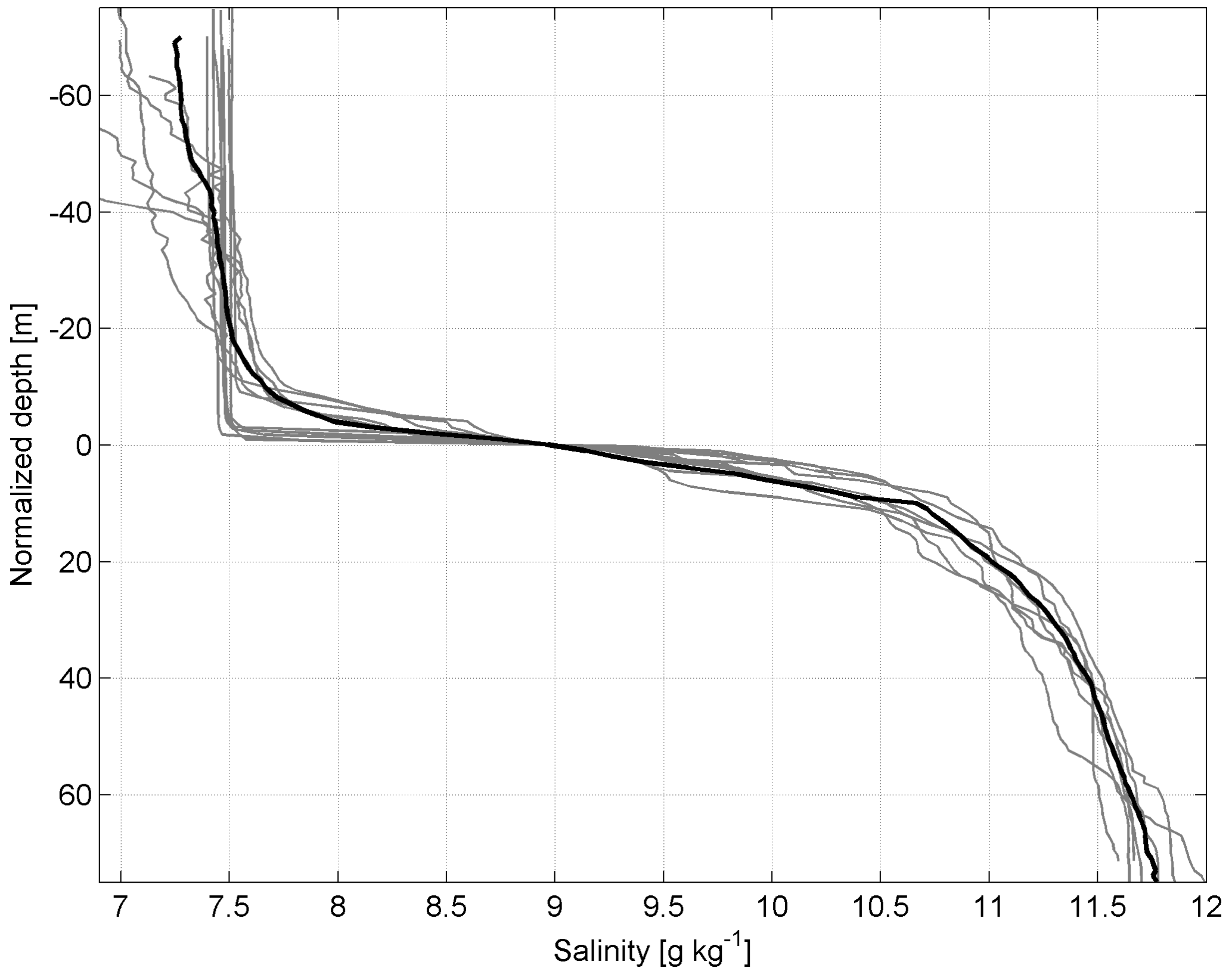
Figure 2 Vertically normalized salinity profiles from 30 January to 4 August 2020 in the northern Baltic Proper (see Fig. 1b). The bold black line represents the mean salinity profile.

In this study the x axis is positive eastward, the y axis is positive northward, the z axis is positive upward (z=0 at the sea surface), and u and v are horizontal velocity components.

The baroclinic components of the geostrophic velocity (u_g and v_g) can be deduced from the hydrographic data. Considering the dynamic method, the geostrophic relationships are as follows.

$$\begin{array}{c}{\displaystyle }{v}_{\mathrm{g}}={\displaystyle \frac{\mathrm{1}}{f}}{\displaystyle \frac{\partial \mathrm{\Phi }}{\partial x}}\\ {\displaystyle }{u}_{\mathrm{g}}=-{\displaystyle \frac{\mathrm{1}}{f}}{\displaystyle \frac{\partial \mathrm{\Phi }}{\partial y}}\end{array}$$

The geopotential, Φ, is proportional to the dynamic height, D, as

$$\mathrm{\Phi }=gD,$$

where g is the gravitational acceleration and f is the Coriolis parameter.

The dynamic height can be determined from the temperature and salinity (density) profiles.

The relative geostrophic velocity was evaluated using dynamic height anomaly relative to a reference pressure (McDougall and Barker, 2011). The geopotential slope of an isobaric surface expresses the horizontal pressure gradient. A zonal glider track enabled calculating the meridional velocity profile of the geostrophic flow. The meridional geostrophic velocity was also calculated from the GETM simulation data. The reference level was set at 70 dbar. The shallower profiles were included using the stepped no-motion level method described in Rubio et al. (2009). Since velocity is not zero at the 70 dbar level, the calculated geostrophic velocities V_{GEO-DENS-glider} and V_{GEO-DENS-GETM} described in Sect. 3.1 represent velocities relative to the no-motion 70 dbar level. Both variables represent an averaged velocity at an extent of 10 km zonal scale around the ADCP position.

To compare the simulated geostrophic velocity profiles with the measured ADCP velocity profiles, the relative geostrophic velocity at the sea surface (calculated relative to 70 dbar using simulated density profiles) was aligned with the geostrophic velocity due to the sea level gradient from the model simulation (V_GEO-SL-GETM). The sea level gradient was estimated from linear regression fit of sea level anomalies at a horizontal scale of 10 km. The difference (vector) between the density-estimated and the sea level estimated geostrophic velocity at the sea surface was applied to the whole geostrophic velocity profile under the assumption that the geostrophic current at the surface is determined by the differences in the sea level exclusively. Adjusted geostrophic velocity profiles are presented as V_GEO-ADJ-GETM in Sect. 3.2.

The direct influence of wind forcing on the subsurface currents was ascertained using the classical Ekman model based on the balance of the frictional and Coriolis forces (Ekman, 1905). The wind stress vector τ as the Ekman model input parameter was calculated using ERA5 (Fig. 1b and c) wind data: $\mathit{\tau }={\mathit{\rho }}_{\text{air}}\text{cd}\left|\mathbf{\text{U}}\right|\mathbf{\text{U}}$, which was previously low-pass-filtered with a cut-off of 36 h to exclude periodic processes. Here U is the wind velocity vector at 10 m height, cd is the drag coefficient and was parameterized as proposed by Wu (1980) as $\text{cd}=(\mathrm{0.8}+\mathrm{0.065}|\mathbf{\text{U}}\left|\right)\times {\mathrm{10}}^{-\mathrm{3}}$, $\left|\mathbf{\text{U}}\right|$ is the wind velocity vector module, and ρ_air is the density of air. The eddy viscosity used in the model was calculated according to Csanady (1981): $\mathit{\nu }=\left|\mathit{\tau }\right|/\mathrm{200}f$, where $\left|\mathit{\tau }\right|$ is the wind stress vector module. The model outputs are the vertical profiles of wind-induced current velocity components.

The temporal development in the vertical current structure is presented as the time series of vertical current shear squared: $s^{\mathrm{2}}=(\partial u/\partial z{)}^{\mathrm{2}}+(\partial v/\partial z{)}^{\mathrm{2}}$.

Persistency of the current, characterizing the variability of the direction of the flow, is defined as the ratio between vector and scalar current speeds:

$$R={\displaystyle \frac{\sqrt{u^{\mathrm{2}}+v^{\mathrm{2}}}}{\frac{\mathrm{1}}{N}\sum \sqrt{u_n^{\mathrm{2}}+v_n^{\mathrm{2}}}}},$$

where u and v in the given formula are the current velocity components' mean values. Current and wind velocity components are presented as 36 h and 10 d low-pass time series. The fourth-order Butterworth filter was used for low-pass filtering.

3 Results

3.1 Boundary current under variable wind forcing

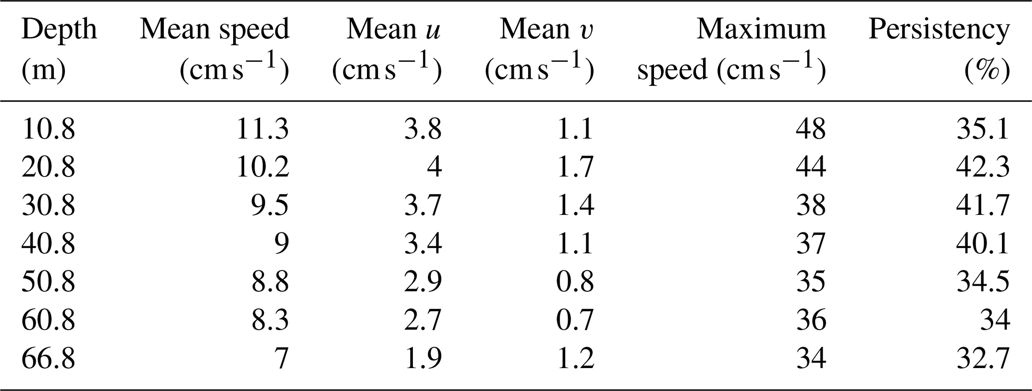
Statistics for the 6 months (1 March–1 September 2020) of ADCP current data revealed the persistency of currents between 32 % and 42 %, with the highest persistency in the 20–40 m depth range (Table 1). Mean and maximum hourly measured speeds were higher in the uppermost bin at 11 m depth as well as 11 and 48 cm s⁻¹, respectively, and lower in the near-bottom layer at 7 and 34 cm s⁻¹. The mean u and v components were positive at all depths, showing the mean flow to the NE sector.

Table 1 Statistics of the 1 h average ADCP current data from 28 February to 2 September 2020.

From the flow structure point of view the ADCP current velocity time series can be divided into two periods: (1) from March until mid-April when the barotropic regime prevailed and (2) from mid-April until September when layered flow dominated (Fig. 3a and b). One can also see the coincidence of the current u and v components in the uppermost and deepest bin during the first period (Fig. 3c and d) except a short period at the end of March. Discrepancies between the two layers afterwards illustrated the layered, baroclinic nature of the flow. The flow regime reacted well to wind forcing. Barotropic flow to the northeast prevailed as a result of southwesterly winds until mid-April (Fig. 4). Only during the last week of March, when wind was from northerly directions was a strong southerly current observed. Similar temporal patterns appeared in the upper layer in the stratified period. Alteration of positive and negative meridional velocities was related to the prevailing wind direction. These tendencies were evident at both the ADCP and Valeport locations. The deep layer current was directed to the east, i.e., onshore, when southerly flow occurred in the upper layer and to the west or southwest when the current to the northeast prevailed. These are signs of the layered structure of the coastal upwelling and downwelling.

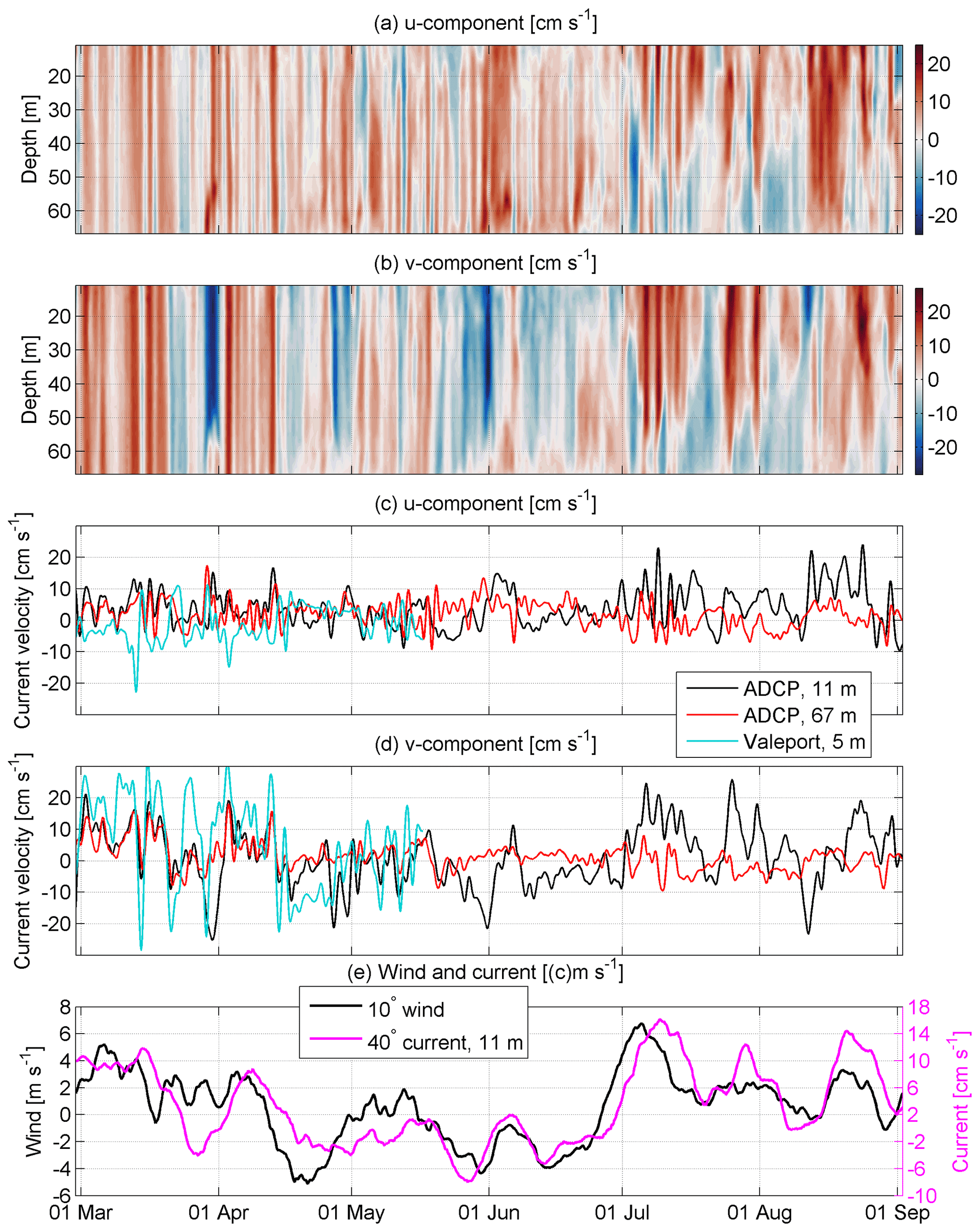
Figure 3 Temporal course of the low-pass-filtered (36 h) current velocity u component (positive eastward, a and c) and v component (positive northward, b and d) in the water column (a and b) as well as in the upper (11 m depth) and deep layer (67 m depth, c and d) at the ADCP and Valeport locations in 2020 (Fig. 1). Low-pass-filtered (10 d) wind 10^∘ component and current 40^∘ component at 11 m depth at the ADCP location (e).

Figure 4 Time series of the 10 m level ERA5 wind data from 1 March to 31 August 2020. Four selected periods are shown: (1) prevailing southwesterly wind, 1–21 March; (2 and 3) prevailing northerly wind, 27 May–4 June and 10–25 June; (4) prevailing southwesterly wind, 2–10 July. The green dotted line marks the beginning and the red dashed line marks the end of the period. Wind data were smoothed with a 36 h filter. The color scale shows wind speed in meters per second (m s⁻¹).

The most frequent current direction in the upper layer (at a depth of 11 m) was 40^∘ at the ADCP location. To estimate the relationship between the low-frequency (10 d low-pass) current component and wind, we calculated the correlation between the 40^∘ current velocity component (c₄₀) in the upper layer and wind speed from different directions with different time lags. The best correlation (r²=0.65, $p<{\mathrm{10}}^{-\mathrm{100}}$, n=4473) was found with the wind from the south, specifically towards 10^∘ (w₁₀), applying a 3 d time lag. This, on the one hand, corresponds to Ekman's theory; however, on the other hand, the 3 d delay is rather long. It can probably be explained by the mixed effect of wind on the surface currents. The momentum flux created by wind impacts the current field fast. The correlation without delay is relatively high (r²=0.55, $p<{\mathrm{10}}^{-\mathrm{100}}$, n=4473) as well. The flow resulting from the sea level gradient and due to the inclination of isopycnal surfaces is also a consequence of wind but develops slower.

Time series of c₄₀ reveal negative values from mid-April until the end of June (Fig. 3e). Before mid-March and in July–August, the c₄₀ was mostly positive. The main course of w₁₀ and c₄₀ coincided well, but discrepancies occurred in the details. For instance, negative c₄₀ occurred when w₁₀ was positive in the ADCP location in the last third of March and first half of May. The mean values of w₁₀ and c₄₀ during the measurements were 0.6 and 3.2 cm s⁻¹, respectively. The w₁₀ is higher in winter and smaller in summer. Considering the linear relation between the two variables, the 1979–2020 mean w₁₀=1.1 m s⁻¹ corresponds to c₄₀=4.2 cm s⁻¹.

At the Valeport location, the most frequent current direction was 350^∘. The discrepancy between the dominant flow direction at the ADCP and Valeport locations is related to the topographic features (Fig. 1). However, from the wider Baltic Sea dynamics point of view the meridional current component is important to investigate. To study the temporal developments of the meridional current, we next analyze the measured and simulated meridional current components at 11 m depth at the ADCP location: V_ADCP and V_GETM. We also calculated the geostrophic meridional component V_GEO-SL-GETM of the current velocity from the simulated sea level gradient and relative geostrophic meridional current component (V_{GEO-DENS-GETM}) at 11 m depth based on simulated temperature and salinity data in the section. The relative geostrophic meridional component (V_{GEO-DENS-glider}) was calculated using the glider temperature and salinity data as well. We also calculated mean Ekman current u and v components in the depth range 0–10 m: U_Ekman and V_Ekman, respectively. All parameters are 36 h low-pass-filtered.

Overall, the simulated V_GETM follows the temporal changes in measured V_ADCP reasonably well (Fig. 5). V_GETM tends to have smaller values than V_ADCP, which means that the meridional component of simulated velocity is biased southward. Sometimes, e.g., in June and August, the discrepancies are considerable. The geostrophic meridional current component V_{GEO-DENS-GETM} was very small, and V_{GEO-DENS-glider} was practically zero in March (Fig. 5b) as the water column was mixed down to the reference depth of the geostrophic current calculation. Since the end of March, overall temporal developments in the meridional current components (V_ADCP and V_GETM) and its geostrophic meridional components (V_{GEO-DENS-GETM}, V_GEO-SL-GETM, and V_{GEO-DENS-glider}) in August match quite well (Fig. 5a and b). This can be related to the multiple effects of wind. Southwesterly wind resulted in the Ekman current towards the eastern coast of the northern Baltic Proper. This first caused a sea level gradient across the basin (higher near the coast), which induced a barotropic current to the north. Secondly, it induced downwelling along the coast and resulted in a vertical gradient of the geostrophic current. Such events were detected at the beginning of April and July, when strong southwesterly winds blew (Fig. 4) and caused an Ekman current towards the coast (Fig. 5c). Northerly or northeasterly winds caused opposite effects. Sea level was lower near the coast compared to offshore and the thermocline was located at shallower depths near the coast. Thus, the flow was directed to the south in the surface layer. Such events occurred in late March and mid-August. Most of the major events of the positive V_ADCP and V_GETM were associated with the positive u component of the Ekman current (see Fig. 5a and c), i.e., flow towards the shore, not along the shore. Thus, the strong wind-driven coastal current to the north is not induced by the direct momentum flux created by wind stress but is rather the result of the wind-driven sea level gradient and depression of the pycnoclines at the coast, which resulted in a vertically sheared geostrophic current.

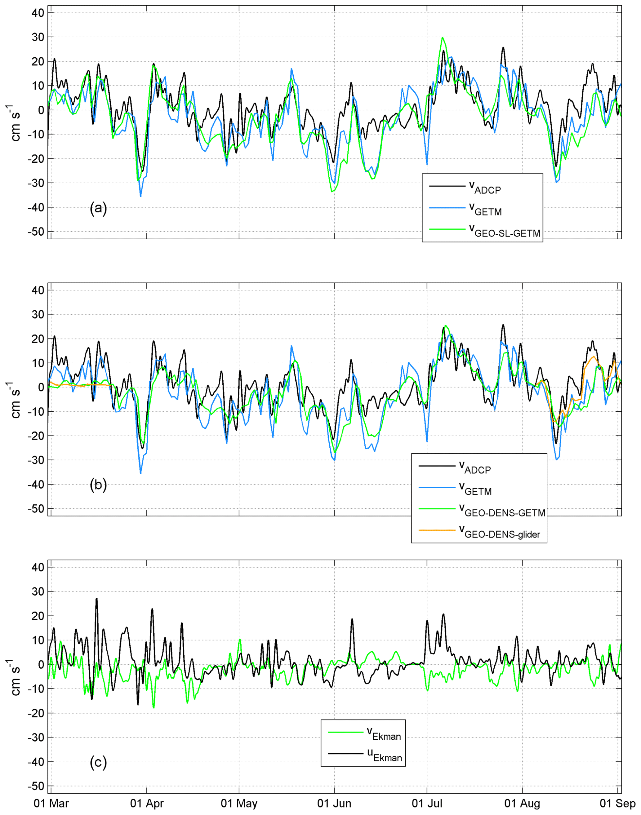
Figure 5 Temporal courses of (a and b) the current velocity v component (positive northward) measured by ADCP (V_ADCP) and the simulated v component (V_GETM) estimated from the GETM sea level data (V_GEO-SL-GETM), from temperature and salinity data collected by a glider (V_{GEO-DENS-glider}), and from temperature and salinity data simulated by GETM at 11 m depth (V_{GEO-DENS-GETM}). Mean Ekman current u component (positive eastward) and v component (U_Ekman as well as V_Ekman) in the depth range 0–11 m (c). Time series are shown from March to September 2020 at the ADCP location (see Fig. 1b and c).

Next, we consider the relationship between the vertical maxima of the current shear and the vertical location of pycnoclines – the seasonal thermocline and halocline. The seasonal thermocline began to develop from the beginning of May (Fig. 6a). The temporal course of salinity at 67 m depth (Fig. 6b) and depth of the halocline center (Fig. 6d) showed that the halocline was mostly located deeper than the deepest ADCP bin. At the end of March, the halocline center reached 55 m depth (Fig. 6d) and high current shear values were observed below 45 m depth (Fig. 6c). The shallower halocline was related to the northerly wind event (Fig. 4), which caused offshore Ekman transport in the upper layer and compensating onshore flow in the deep layer (Fig. 3). Such events of high current shear in the deep layer also occurred at the end of April to early May, from the end of May to mid-June, and in mid-August (Fig. 6c) when the halocline center was shallower and salinity increased at 67 m depth. Note that the depth of the halocline center and shear maxima was vertically shifted, and the halocline center was deeper. This can be explained by the vertical range of the halocline. The upper boundary of the halocline is shallower than the center of the halocline. Thus, the shear maxima were rather linked to the upper boundary of the halocline.

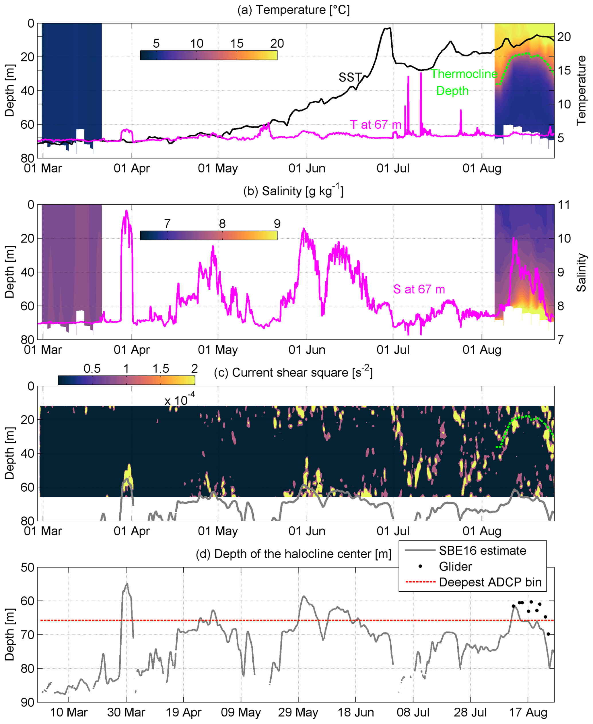
Figure 6 Temporal courses of temperature, salinity, current shear squared, and halocline depth at the ADCP location from March to September 2020 (see Fig. 1b and c). (a) Temporal course of sea surface temperature (SST) and temperature at 67 m depth; temporal course of the vertical distribution of mean temperature in March and August calculated from glider data (color scale). The depth of the thermocline center is shown as a red dashed line. (b) Temporal course of salinity at 67 m depth; temporal course of the vertical distribution of mean salinity in March and August calculated from glider data (color scale). Mean temperature and salinity profiles were calculated for each glider passing within the 3.7 km zonal window around the ADCP location. The depth of the thermocline center is shown as a red dashed line. (c) Temporal course of the vertical distribution of current shear squared and depth of the halocline center (grey line). (d) Depth of halocline center calculated from SBE16 data and in August from glider data. The depth of the deepest ADCP bin is also shown (red dotted line).

Stronger and more extensive shear maxima in the upper part of the water column were observed since late April (Fig. 6c). They appeared days before thermal stratification developed. One could see that SST (sea surface temperature) and temperature at 67 m depth coincided until the end of April. The occurrence of earlier shear maxima could be explained by the formation of the stratification in the upper layer caused by the transport of fresher surface water to the area due to northerly wind forcing. Shear maxima became stronger in the second half of May when thermal stratification developed. Strong downwelling and vertical mixing occurred in July as a result of a strong southwesterly wind impulse with a duration of more than a week (Fig. 4). This can be seen as a drop in SST from 21 to 15 ^∘C and occasional high temperature recordings in the deep layer (Fig. 6a). The latter indicates that the upper layer water arrived at the 67 m deep measurement spot. This event is well reflected in the time series of current shear. Deepening of the shear maxima down to 50–55 m depth (Fig. 6c) occurred together with thermocline deepening, as the near-bottom temperature recordings suggest. A precondition for such a rapid drop in SST was the formation of a thin and exceptionally warm surface layer due to atmospheric heat flux (Fig. 6a) and weak wind (Fig. 4) at the end of June. Relaxation of the downwelling occurred in mid-July, and another downwelling developed at the end of July. The linkage between the thermocline and shear maxima was clearly seen in August when glider observations were available (Fig. 6c). The thermocline and shear maxima reached down to 40 m depth at the beginning and the end of the month, while they were located at 20 m depth in the middle of the month (Fig. 6a and c). The vertical movements of the halocline (Fig. 6d) and thermocline (Fig. 6a and c) as well as linked shear maxima were synchronized. Like the thermocline, the halocline also had a shallower position in mid-August and was deeper before and after. Note that downwelling was initiated by strong southerly, southwesterly, or westerly winds and all events were seen as a SST decrease, likely due to vertical mixing, a decrease in salinity at 67 m depth, and deepening of the thermocline and halocline as well as related shear maxima. Relaxation of downwelling occurred when northerly winds or calmer periods prevailed and appeared as an increase in SST and upward movement of both pycnoclines.

Thus, we can conclude that the vertical structure of currents was strongly linked to the varying depths of pycnoclines, which were sensitive to wind forcing.

3.2 Quasi-permanent circulation patterns

In the previous section, we demonstrated the importance of wind forcing and stratification for the currents. Next, we describe the current structure during the quasi-steady forcing periods. We have selected four periods of 8–21 d duration with relatively stable forcing (see Fig. 4) to analyze the mean measured and simulated flow structure at the ADCP and Valeport locations (Fig. 7) and along the zonal section (Fig. 8). Likewise, we investigated the horizontal structure of simulated flow in the three forcing cases in three layers: upper layer (5 m), intermediate layer (40 m), and deep layer (110 m) (Figs. 9–11).

Figure 7 The mean resultant wind vectors (a, e, i, m), mean profiles of current velocity vectors calculated from ADCP data (black arrows, b, f, j, n), and mean simulated current velocity vectors at the ADCP location (c, g, k, o) are shown for selected periods (Fig. 4). The mean current velocity vector at 5 m depth based on Valeport data (b, red arrow) and mean simulated current velocity vector at the Valeport location (c, red arrow) for the first time period are shown. In the right panels, mean adjusted geostrophic velocity vectors V_GEO-ADJ-GETM (d, h, i, q) are shown.

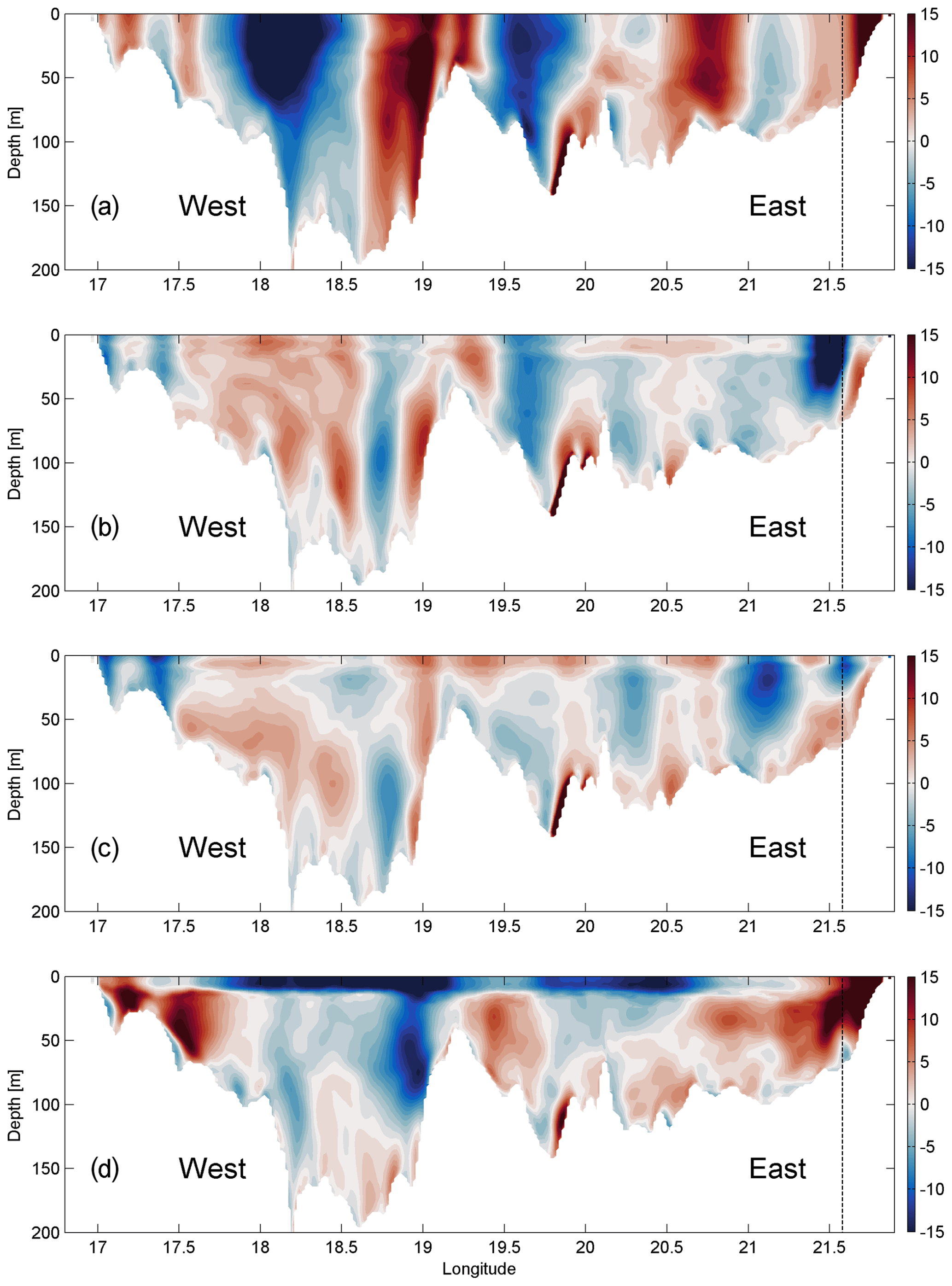
Figure 8 Vertical distribution of simulated mean meridional current velocities for four selected periods: (a) 1–21 March, (b) 27 May–4 June, (c) 10–25 June, and (d) 2–10 July 2020 (see Fig. 4) along the ADCP deployment latitude (Fig. 1b). The color scale displays meridional velocity (positive northward) in centimeters per second (cm s⁻¹). Vertical dotted lines show the ADCP location.

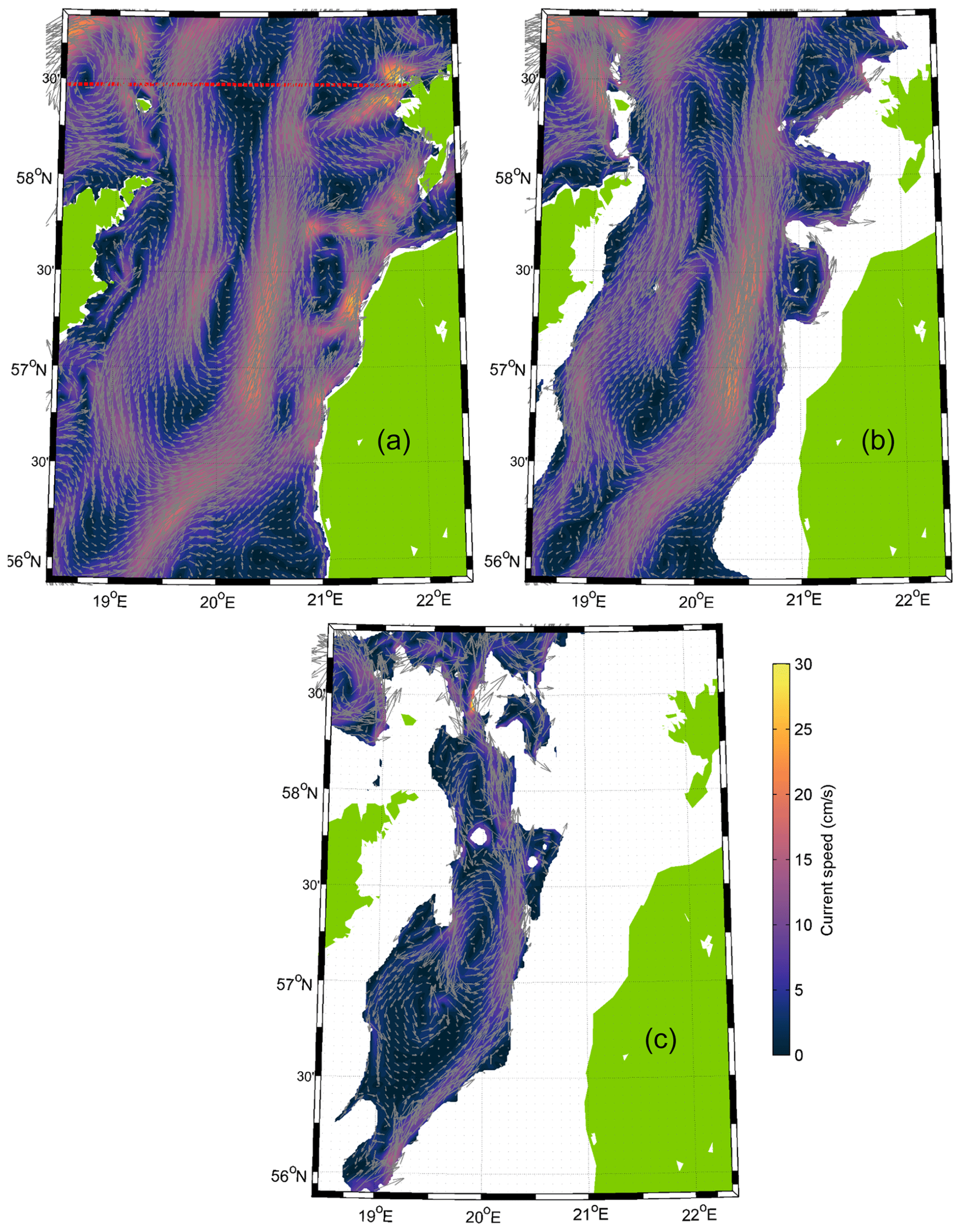
Figure 9 Mean simulated currents in the case of prevailing southwesterly winds from 1 to 21 March 2020 without the thermocline at 5 (a), 40 (b), and 110 m depth (c). The color scale shows current speed in centimeters per second (cm s⁻¹). The red dashed line in panel (a) shows the location of the transect presented in Figs. 8 and 12.

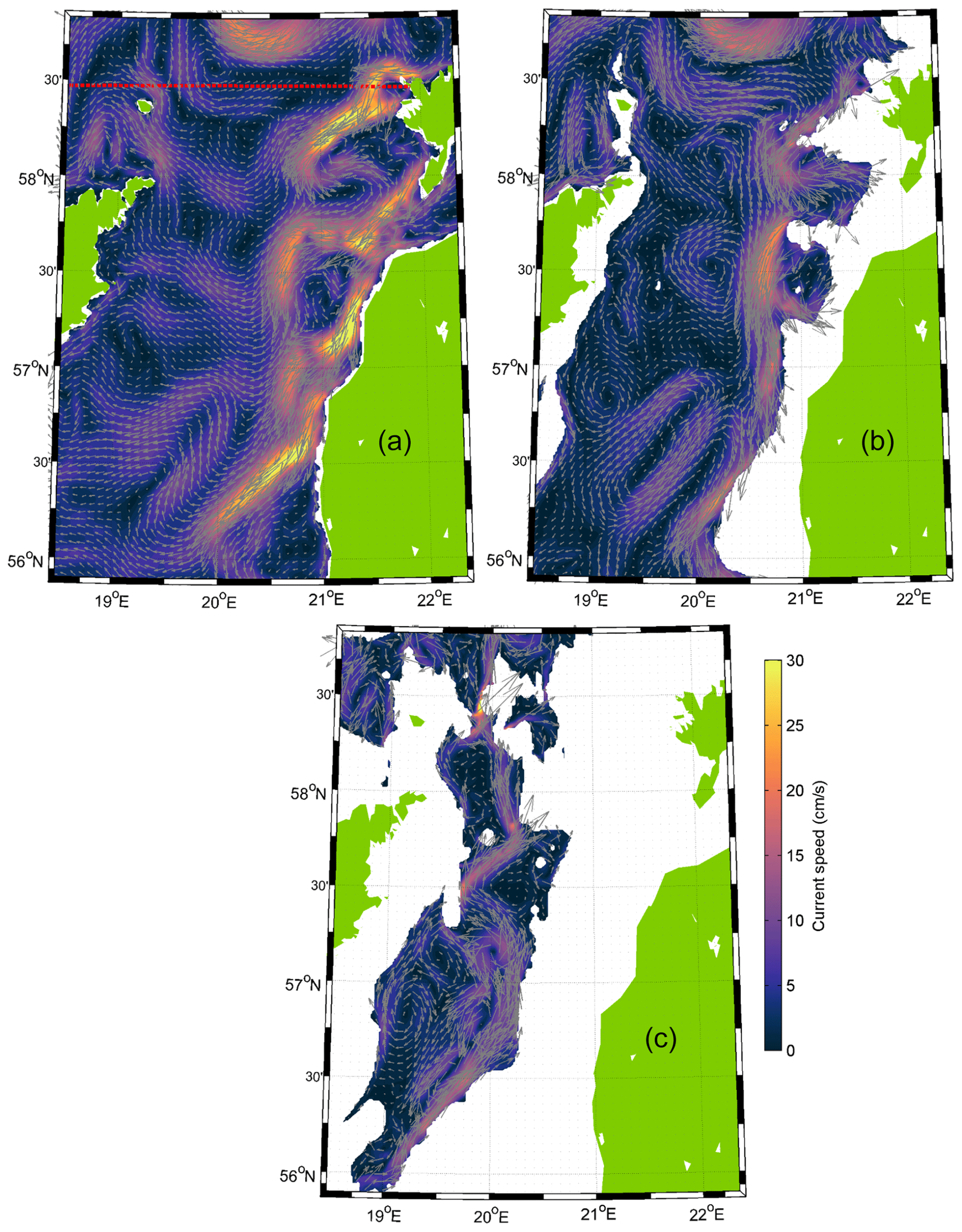
Figure 10 Mean simulated currents in the case of prevailing northerly winds from 27 May to 4 June 2020 with the thermocline at 5 (a), 40 (b), and 110 m depth (c). The color scale shows current speed in centimeters per second (cm s⁻¹). The red dashed line in panel (a) shows the location of the transect presented in Figs. 8 and 12.

Figure 11 Mean simulated currents in the case of prevailing southwesterly winds from 2 to 7 July 2020 with the thermocline at 5 (a), 40 (b), and 110 m depth (c). The color scale shows current speed in centimeter per second (cm s⁻¹). The red dashed line in panel (a) shows the location of the transect presented in Figs. 8 and 12.

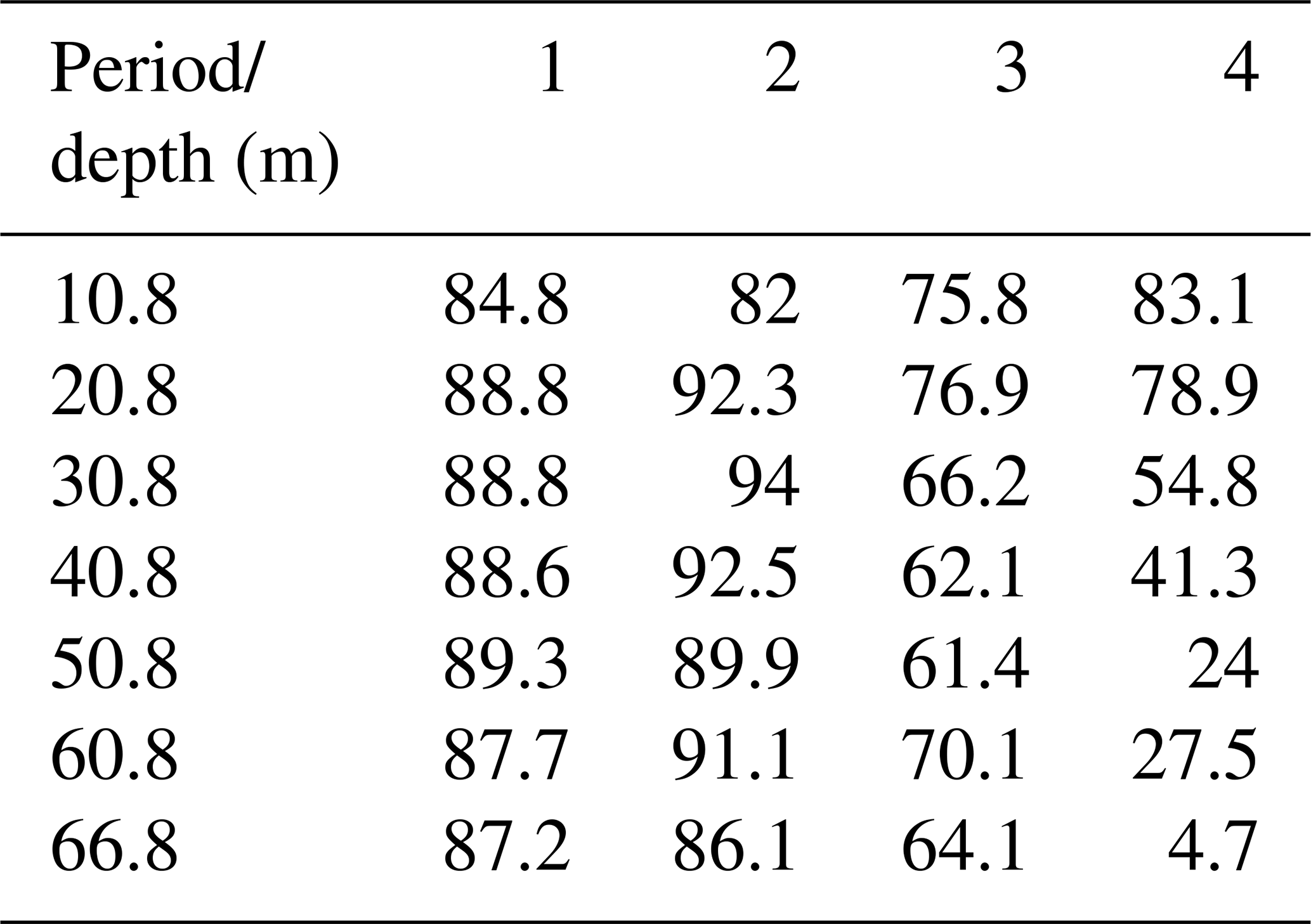
The persistency of the measured currents at the ADCP location was very high in all selected periods (Table 2). Only during the fourth period was the persistency lower than 50 % below the seasonal thermocline. Particularly high persistency (82 %–94 %) occurred in the first and second periods. Thus, measured currents during the quasi-steady forcing have much higher persistency than overall in the time series (see Table 1).

Table 2 Persistency (%) of the measured currents at the ADCP location at the selected depths during the selected periods: 1 to 21 March (1); 27 May to 4 June (2); 10 to 25 June (3); 2 to 10 July (4) 2020.

Barotropic flow to the northeast prevailed throughout the water column at the ADCP location in the first period (1–21 March) when southwesterly wind prevailed (Fig. 7a–c). An even stronger mean current to the north-northwest was registered at 5 m depth at the Valeport location (Fig. 7b). The latter indicates the boundary effect near Saaremaa Island, and the current was directed along the coast (Fig. 1c). Mean flow was to the south in the upper layer (Fig. 7g) during the second period (27 May–4 June) when northerly wind prevailed (Fig. 7e), to the southeast below the thermocline, and to the east below the halocline (Fig. 7f and g). In general, a similar current pattern occurred in the third period (10–25 June) when northwesterly wind prevailed (Fig. 7i–k). Due to relatively strong southwesterly wind forcing in the fourth period (2–10 July), flow to the northeast prevailed in the upper layer and to westerly directions below the thermocline (Fig. 7m and n).

In conclusion, a pattern typical for the downwelling event – a current to the northeast along the boundary and towards the shore in the upper layer (Fig. 7n and o) as well as a seaward current to the southeast in the deep layer (Fig. 7n) – occurred during southwesterly wind domination (Fig. 7m). On the contrary, a pattern typical for the upwelling, with the flow to the south along the coast in the upper layer (Fig. 7g and k) and onshore (east) in the deeper layers (Fig. 7f, j, g, and k), was observed in the case of northerly winds (Fig. 7e). These vertical patterns (downwelling and upwelling) of the current velocity were also well captured by the numerical model. The stronger mean measured current at 5 m depth near the boundary (Valeport location) was well reproduced by the model (Fig. 7b and c). The mean adjusted geostrophic velocity profiles based on simulation data had a quite similar vertical structure compared to the measured mean velocity profiles in all periods (Fig. 7, second and fourth columns). Thus, currents were generally in geostrophic balance during the quasi-steady periods. The transition from one state to another likely has an ageostrophic nature, as wind is the main driver for the change.

Next, to understand the larger-scale circulation dynamics during the periods, we analyze the vertical structure of the mean meridional component of currents (Fig. 8) in the section along the latitude of the ADCP location (Fig. 1b) and the horizontal structure of mean currents at selected depths (Figs. 9–11) in the eastern Gotland Basin (Fig. 1b) using simulated current data. The current data are averaged within the same time windows with relatively stable wind forcing as analyzed above.

The structure of the meridional component of currents in the section is characterized by high spatial and temporal variability (Fig. 8). Unidirectional flow prevailed in most of the section down to the halocline or even deeper in the case of no thermal stratification and southwesterly winds (first period) (Fig. 8a). The northward current along the eastern boundary with a cross-coast extent of 10 km was especially strong. This strong boundary current was also registered by the Valeport (Fig. 3d). The strong maxima of the northward flow can be found at 20.5–21.0, 18.6–19.3, and around 17.6^∘ E. The strong southward flow prevailed at 21.0–21.3, 19.4–20.0, and 17.6–18.6^∘ E. Horizontal flow structure in the eastern Gotland Basin consisted of the two stronger current zones above the halocline (at a depths of 5 and 40 m), the northward current along the eastern bottom slope, and the southward current along the bottom slope in the western part of study area (Fig. 9a and b). The two zones were connected with several cyclonic cells. The northward flow below the halocline at a depth of 110 m (Fig. 9c) coincided with the flow in the upper layer along the bottom slope in the eastern Gotland Basin area but was forced to the westward trajectory by bathymetry in the northern area.

The mean meridional current patterns were very similar in the following two periods (second and third) with prevailing northerly winds and the presence of thermocline. In both cases, the zonal scale of the southward flow around the ADCP location was 10–15 km (Fig. 8b and c). The flow did not extend to the eastern boundary, and a narrow northward flow with a width of 5–10 km occurred along the coastal slope. The width of the southward flow near the western boundary of the section was about 30 km. In between, several circulation cells with zonal scales of 20–60 km can be distinguished in the cross-section (Fig. 10a). The horizontal structure of the flow below the thermocline at a 40 m depth in the eastern Gotland Basin revealed a strong southward current in the eastern part of the area in the second period (Fig. 10b). The current swirled, split into two branches, and re-merged back to one in several locations. The southward flow below the thermocline (40 m depth) coincided with the offshore branch in the upper layer in the central area of the basin (Fig. 10a and b). Sub-halocline flow revealed the strongest northward current along the bottom slope and the strongest cyclonic cell in the eastern Gotland Basin among the selected periods (Fig. 10c).

The flow pattern in the case of strong southwesterly dominance (fourth period) under stratified conditions revealed a strong northward current component along both boundaries of the section (Fig. 8d). In between, the strong southward flow occurred in the surface layer. Similarly to the northerly wind prevailing, a complicated three-layer structure with variable horizontal patterns in the zonal scale of 20–60 km occurred. Flow to the southeast prevailed for most of the study area in the upper layer (5 m depth), except in the eastern boundary zone, where a strong northeastward downwelling-related flow occurred (Fig. 11a), as also was observed in our ADCP mooring data (Fig. 7n). A strong current also occurred in the Irbe Strait towards the Gulf of Riga. Downwelling-related flow along the eastern coast was also observed at 40 m depth (Fig. 11b). In the deep layer below the halocline (110 m depth), a northward current along the eastern bottom slope and cyclonic cells in the eastern Gotland Basin were observed (Fig. 11c).

Due to seasonality in forcing, variations in the circulation on this timescale can be expected. Next, we analyze the vertical distribution of the monthly mean (April, July, and December) and annual mean meridional velocity component (Fig. 12) along the zonal section (Fig. 11) at ADCP latitude based on simulation data from September 2010 to August 2020. The boundary current along the eastern coastal slope occurred year-round (Fig. 12d) but was the strongest in winter (Fig. 12c). This is related to the wind regime: southwesterly winds prevail more in winter but are less frequent in spring and summer. The seasonal signal can be found in the whole section (Fig. 12a–c). Well-defined large cyclonic gyres in the northern Baltic Proper can be found in winter (Fig. 12c), while in spring and summer (Fig. 12a and b), the mean current structure is characterized by smaller-scale zonal features and weaker flow. However, it is noteworthy that the mean flow is to the north along the eastern coastal slope in all seasons.

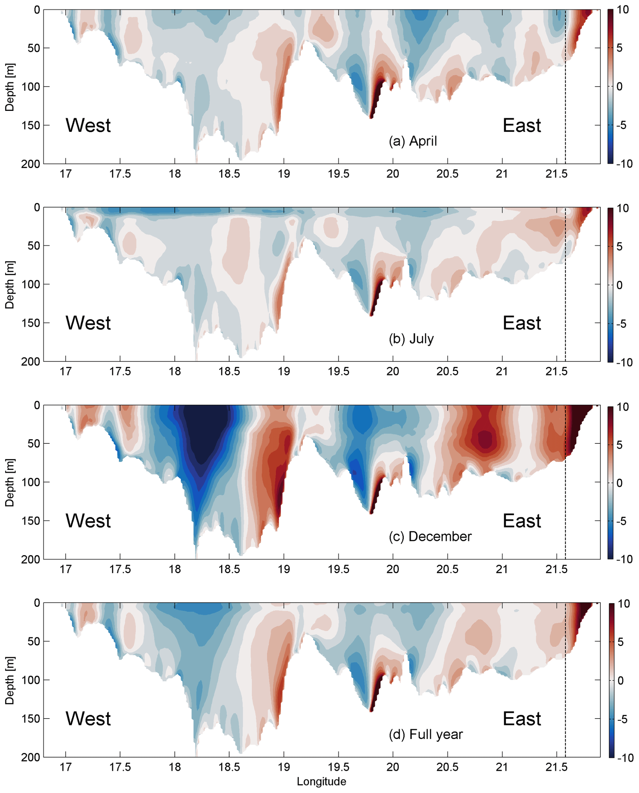
Figure 12 Vertical distribution of monthly mean (April, July, and December) and annual mean meridional velocities (positive northward) along the zonal section at ADCP latitude based on simulation data from September 2010 to August 2020. The color scale shows meridional velocity in centimeters per second (cm s⁻¹). Vertical dotted lines show the ADCP location.

3.3 Sub-halocline current

As shown above, a cyclonic gyre was present below the halocline in the eastern Gotland Basin in all selected periods (Figs. 9–11). The flow in this cyclonic system was especially strong along the eastern slope of the eastern Gotland Basin. The northern branch of this circulation system is connected to the clearly distinguishable northward current. The position and magnitude of the current varied under different conditions. The current was stronger and meandered to west in the shallower area between Gotland and Fårö Deep in the case of northerly wind, while it was slower and the meandering did not occur in the case of southwesterly winds. To confirm the simulated cyclonic circulation in the eastern Gotland Basin and the northward-flowing current towards the Nothern Deep, the Argo float trajectory and the mean current field between 105 and 135 m depth were plotted in the same time frame from 15 August 2013 to 15 August 2014 (Fig. 13a). The general features in the simulated mean currents and the Argo float trajectory agreed well. The Argo float first completed two circles (smaller and larger) in the eastern Gotland Basin and then headed to the north. The float arrived and was recovered in the shallower area between the Fårö and Nothern Deep. This sill is an important location for the deep layer water renewal in the northern Baltic Proper, as this is the only remarkable passage to the north below 100 m depth (see bathymetry in Fig. 1b). The sill is located slightly south of the selected section along the latitude of the ADCP deployment.

Figure 13 Mean current field between 105 and 135 m depth based on simulation data and Argo (WMO number 6902014) float trajectory during the period 15 August 2013–15 August 2014 in the deep layer (within its parking depth range of 105–135 m, shown in red). Only one longer period occurred when the float drifted on the surface (shown in white). The color scale shows current speed in centimeters per second (cm s⁻¹).

The mean simulated meridional flow to the north over the still was concentrated in a narrow cell with a zonal scale of 5–6 km in 2010–2020 (Fig. 14a). The flow was especially strong when northerly winds prevailed, e.g., in the second period from 27 May to 4 June 2020 (Fig. 14b). The mean density field sloped downward to the left (west) of the flow (Fig. 14a and b), which is typical for a gravity current. The meridional current velocity (C_T) in the trench was mostly positive (northward) and in the range of 10–20 cm s⁻¹ during the study period March–September 2020 (Fig. 14c). The C_T was reversed in the first half of July, which coincided with the strong southwesterly wind impulse (Fig. 4). The time series of C_T for 2010–2020 (Fig. 14d) revealed many reversal events, but the long-term mean meridional velocity was 10 cm s⁻¹ to the north. Reversals were most frequent in November–December when the monthly mean southward C_T was 6–7 cm s⁻¹ and rarer in March–May when monthly averages were in the range of 12–14 cm s⁻¹. Thus, the deep layer water renewal in the northern Baltic Proper is most active in the spring period and more restricted in late autumn–early winter. The best correlation (r²=0.25, $p<{\mathrm{10}}^{-\mathrm{100}}$, n=3838) between 10 d low-pass current velocity at the sill and wind was found with the wind from ENE (70^∘) with a delay of 6 d. This is another confirmation that prevailing southwesterly winds slow down or reverse the C_T and prevent deep water renewal in the northern Baltic Proper.

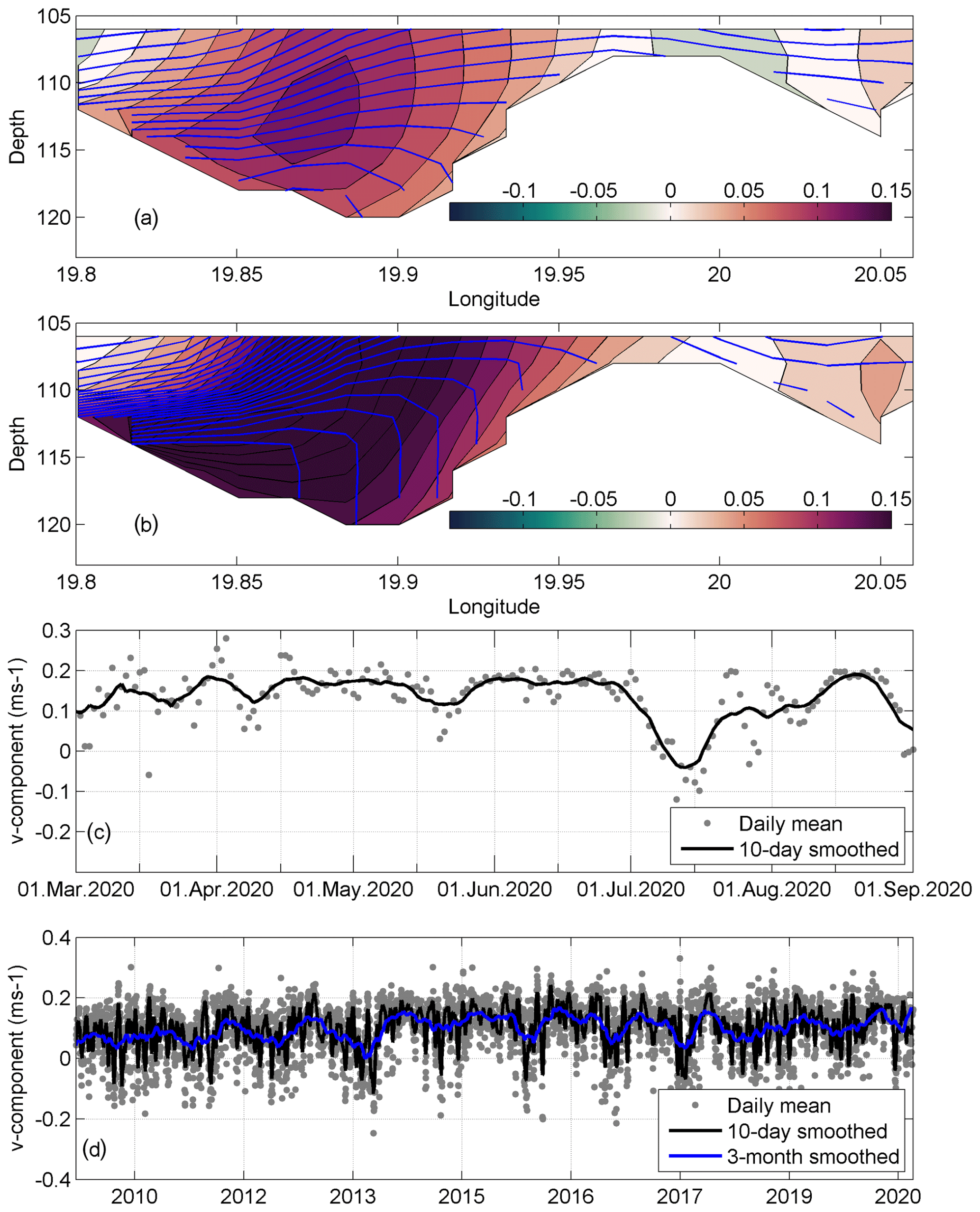
Figure 14 (a) Mean simulated meridional current component v (positive northward) and density isolines at the section below 105 m depth (the section location is shown as a red line in Fig. 1b) in 2010–2020. (b) Mean simulated meridional current component v and density isolines at the section below 105 m depth from 27 May to 4 June 2020 during a northerly wind impulse. In color scale, contours with a step of 2 cm s⁻¹ show the current v component (m s⁻¹, positive northward) and blue lines show density isolines with a step of 0.05 kg m⁻³. (c) Time series of the v component below 105 m at the sill. Dots mark the daily mean and the bold line the 10 d smoothed v component from March to September. (d) Time series of the v component below 105 m at the sill. Dots mark the daily mean; the bold black line marks the 10 d smoothed and the bold blue line the 3-month smoothed v component in the period 2010–2020.

4 Discussion

Moorings carrying ADCPs and single-point current meters, as well as underwater glider surveys, were applied together with numerical modeling to investigate circulation in the Baltic Proper.

Strong linkage between the vertical location of the current shear maxima and the two pycnoclines was observed. The same finding was reported in the Gulf of Finland (Suhhova et al., 2018). The current shear maxima in the Gulf of Finland were related to the along-gulf estuarine circulation and its alterations. In the present case, the shear maxima were related to the currents along the basin axis and the coastal downwelling and upwelling circulation structures. The separation of the cross-shelf flow by a pycnocline has been documented in several other coastal systems (Davis, 2010; Gilcoto et al., 2017; Villacieros-Robineau et al., 2013).

A boundary current in the upper layer along the eastern coast was observed. The current was well correlated with the wind. The wind regime in the area is the combination of the global circulation and specific direction-dependent boundary layer effects, which results in domination of winds along the axis of the Baltic Proper (Soomere and Keevallik, 2001). Along-axis wind causes the Ekman current (Ekman, 1905) to the right of the wind direction in the upper layer, i.e., a flow across the basin axis. The resulting convergence (divergence) in the case of southwesterly (northerly) winds at the eastern coast causes an across-axis sea level gradient and the upper pycnocline inclination, which in turn cause a horizontal pressure gradient and result in a geostrophic flow to the north (south) in the upper layer. Boundary currents forced by the pressure gradient caused by wind-driven divergence and convergence are common in coastal systems (Berden et al., 2020; Longdill et al., 2008; Wu et al., 2013). The geostrophic current velocity agrees well with the total current velocity profiles. Thus, the current along the boundary was generally in geostrophic balance, but across-shore ageostrophic flow created preconditions for this geostrophic coastal current.

Circulation rapidly reacted to the wind forcing. Persistency of the current for 6 months was rather low (30 %–40 %) due to variability in the wind forcing. The estimated persistency from long-term numerical simulation data in the same area above the halocline was 70 %–80 % in 1981–2004 (Meier, 2007) but around 30 %–40 % in the upper layer in 1958–2007 (Jędrasik and Kowalewski, 2019). However, the quasi-steady circulation patterns detected under different wind and stratification conditions were highly persistent, mostly >75 %.

The mean cyclonic circulation in the upper layer of the Baltic Proper has been reported by many modeling studies (Hinrichsen et al., 2018; Jedrasik et al., 2008; Jędrasik and Kowalewski, 2019; Meier, 2007; Placke et al., 2018). However, the magnitude of the long-term mean circulation patterns had a considerably lower magnitude than the quasi-steady circulation structures presented in this study. Likewise, the current direction of quasi-steady patterns varied and differed considerably from the long-term mean. The circulation structures on this timescale also differ from the long-term mean because of seasonal and interannual variations in the forcing. The cyclonic circulation and the eastern boundary current towards the north in the upper layer are stronger in autumn and winter, as noted by previous simulations (Jędrasik and Kowalewski, 2019), when strong southwesterly winds are more frequent (Soomere and Keevallik, 2001). Quasi-steady circulation patterns were characterized by complicated lateral vortices with the zonal scale of 20–60 km. The richness of vortical structures has been suggested by several numerical modeling studies (Dargahi, 2019; Zhurbas et al., 2021). In situ measurements are needed to verify the existence of the vortices and to characterize their effect on the physical and biogeochemical fields in more detail.

Two quasi-permanent circulation features were detected in the deep layer. The cyclonic gyre was present below the halocline in the eastern Gotland Basin, with the strongest flow along the eastern slope, which has been documented by earlier in situ measurements (Hagen and Feistel, 2004, 2007). The northern branch of the eastern Gotland Basin current is connected to the quasi-steady northward-flowing current towards the narrow Fårö sill between the Fårö and Nothern Deep. The width of the current was mostly 10–30 km but only 5 km at the sill. The mean northward component of the current was 10 cm s⁻¹, which can be explained by the mean density structure (Fig. 14a) and is typical for the gravity current in a channel (Zhurbas et al., 2012). This current is an important deeper limb of the Baltic haline conveyor belt (Döös et al., 2004). The current was stronger in the case of northerly winds and weaker during southwesterly wind prevailing. This is typical behavior of the estuarine circulation: up-estuary wind causes weakening or reversal of the deep layer current and down-estuary wind intensification of the estuarine current (Geyer and MacCready, 2014) as observed in the Gulf of Finland (Liblik et al., 2013; Lilover et al., 2017; Suhhova et al., 2018) and several other estuaries (e.g., Giddings and MacCready, 2017; Scully, 2016). In the case of northerly wind, the vertical and horizontal density gradient in the Fårö sill was much stronger (Fig. 14b) than the mean gradient in 2010–2020 (Fig. 14a) according to the simulation. Note that on the right-hand flank, the isopycnals are vertical (Fig. 14b). A similar structure of the gravity current has been measured by acoustic profiling in the western Baltic (Umlauf et al., 2009). The current to the north and potentially the deep layer water renewal in the northern Baltic Proper are more intense in March–May when southwesterly winds are less frequent, and the current is weakest in November–December. If the water that overflows the Fårö sill is dense enough, it occupies the Nothern Deep bottom layers, and the old, oxygen-depleted bottom water is lifted and advected to the Gulf of Finland, as observed during high major Baltic inflow activity (Liblik et al., 2018). If the overflow has a lower density compared to the deep layer waters in the Nothern Deep, it does not dive to the bottom but stays as a buoyant layer.

The most favorable wind for the up-estuary deep layer advection in the Gulf of Finland is from the northeast (Elken et al., 2003). Thus, northerly winds support deep water renewal and strengthening of the stratification all the way from the Gotland Deep to the Gulf of Finland. The deep layer currents are quite well covered by observations in the Gulf of Finland (Lilover et al., 2017; Rasmus et al., 2015; Suhhova et al., 2018). However, observations are lacking from the Gotland Deep to the entrance of the Gulf of Finland. The only in situ record about the feature between Gotland and Nothern Deep is the Argo float track. The Argo trajectory supported our suggestion about the existence of the sub-halocline current to the north. Our simulations suggested that the strength and position of the current did depend on the wind forcing. Observations and simulation results at the channel-like topographic constriction, Slupsk Furrow, in the southern Baltic have shown that the meandering of the gravity current is strongly affected by the bottom topography and wind forcing (Zhurbas et al., 2012). ADCP measurements are needed to understand the behavior of the sub-halocline current better.

Overall, simulated currents agree quite well with the ADCP measurements in the upper layer. However, the meridional component of the simulated current (V_GETM) was biased (Fig. 5a). The mean V_ADCP was 1.1 cm s⁻¹, but the mean V_GETM was −3.2 cm s⁻¹ at 10 m depth during the study period. Such bias could not be found in the deep layer. Flow to the north was often weaker compared to measurements (V_ADCP), and flow to the south was stronger than observed by the ADCP in the upper layer. A similar tendency can be found in a comparison of ADCP measurements and simulation results in the Gulf of Finland (Suhhova et al., 2015). Near the right-hand side coast (looking up-estuary, i.e., to the east in the Gulf of Finland), the down-estuary flow was stronger and more frequent in the simulation compared to the measurements (see their Fig. 2). Interestingly, a similar bias was detected in the deep layer at the eastern flank of the Gotland Deep at 204 m depth (Placke et al., 2018). Four different models considerably underestimated (Placke et al., 2018) the mean flow to the north derived from observations (Hagen and Feistel, 2004). The first possible explanation for the bias could be the smaller width of the boundary current. Indeed, the mean flow towards north in 2010–2020 was stronger in the east from the ADCP location (Fig. 12). The second possible source for the discrepancy could be related to the performance of simulations of ageostrophic or geostrophic flow. We will discuss this further in the next section.

Quite large discrepancies between the simulation and the measurements occurred in June. In the first half of the month, simulation was biased to the south, but in the second half, a bias to the north can be seen (Fig. 5a). In both cases, the geostrophic current seems to play an important role in the discrepancy. Strong simulated V_{GEO-DENS-GETM} to the south (north) occurred in the first (second) part of June. In August, the simulation did not capture the strongest flow event to the north on 21–24 August (Fig. 5a). In the same period, much lower values of the V_{GEO-DENS-GETM} compared to the V_{GEO-DENS-glider} can be seen. These signs suggest, first, that the isopycnals in the model react to the forcing more rapidly than in the sea. Secondly, there is a bias in the across-slope seasonal thermocline inclination. Likely, the thermocline is tilted more towards the surface near the coast in the model than in the sea. We next evaluate the measured (by glider) and simulated temperature, salinity, and geostrophic velocity fields on 11–12 and 22–23 August.

Surface layer geostrophic velocity in the simulation agrees well with the estimates from the glider data on 11–12 August (Fig. 15a and b), though the glider observations reveal sharper thermocline inclination than the simulation. Discrepancies in the temperature, density, and geostrophic current fields on 22–23 August are much larger (Fig. 15c and d). Glider observations revealed that the thermocline depressed down near the coast, which is typical for a downwelling. The inclination in the thermocline caused strong geostrophic flow to the north at the location of the ADCP (Fig. 15c). The homogenous mixed layer reached down to 22 m depth at the easternmost end of the section. Such an inclination, well-defined homogenous layer, and geostrophic current to the north at the ADCP location were not revealed by the simulation (Fig. 15c). Thus, we can conclude that the bias in the boundary current simulation could be related to the inaccuracy of reproducing the temperature and salinity fields as well as the resulting geostrophic component of currents. We will not go into further details of this problem here, as it is out of the focus of the present work. However, conclusions from simulation studies that have focused on the long-term mean current fields in the upper layer, but did not validate simulations with direct current observations, should be considered carefully, as the magnitude of the long-term residual current is very small compared to the magnitude of the currents during the quasi-steady states. We suggest that a dedicated study involving numerous current profiling records should be conducted to track down the causes of the discrepancies between observations and simulations.

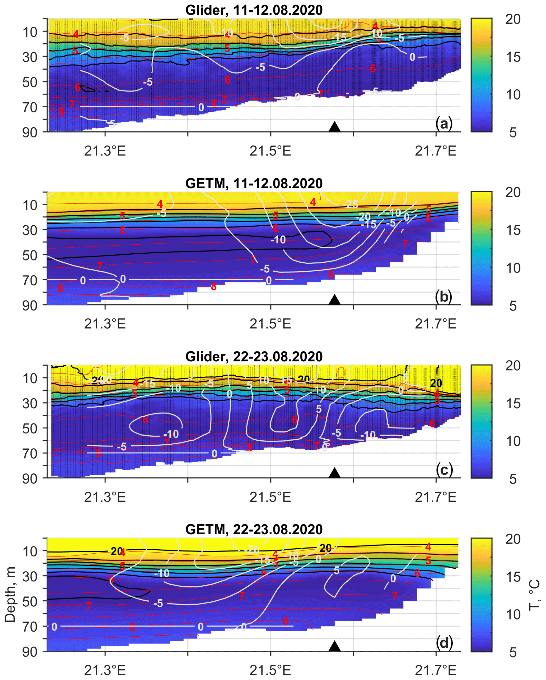
Figure 15 Temperature (color contours), density isolines (red lines), and relative geostrophic current (white lines) based on glider observations and GETM simulation on 11–12 and 22–23 August 2020.

5 Conclusions

A strong link between the existence and location of the two pycnoclines and the current structure was observed. The boundary current was observed in the upper layer along the eastern coast of the Baltic Proper. The current was mainly in geostrophic balance, and across-shore Ekman transport created preconditions for the geostrophic coastal current. The boundary current rapidly reacted to the changes in the wind forcing, which was reflected in a relatively low persistency of currents (30 %–40 %) in the whole water column during the 6-month measurement period. However, the quasi-steady circulation patterns formed under certain wind and stratification conditions were highly persistent (mostly >80 %) and generally in geostrophic balance.

The sub-halocline, quasi-steady northward (towards Fårö sill) gravity current with a width of 10–30 km was detected by the simulation. The finding was supported by the Argo float displacement data. This important deeper limb of the Baltic Sea haline conveyor belt was stronger in the case of northerly winds and weaker during southwesterlies. More detailed studies of the dynamics and water properties of this current are essential to understand the renewal process of deep layer waters in the northern Baltic Proper and in the Gulf of Finland.

Generally, the structure of the boundary current was well reproduced by the GETM. However, the meridional component of the simulated current was biased southward. Further in situ measurements and simulations of the current regimes in various locations during the periods of quasi-steady forcing could help to reveal the causes of the discrepancy.