the Creative Commons Attribution 4.0 License.
the Creative Commons Attribution 4.0 License.
 | 08 Jun 2022
Seasonal extrema of sea surface temperature in CMIP6 models
Yanxin Wang
David P. Stevens
Gillian M. Damerell
CMIP6 model sea surface temperature (SST) seasonal extrema averaged over 1981–2010 are assessed against the World Ocean Atlas (WOA18) observational climatology. We propose a mask to identify and exclude regions of large differences between three commonly used climatologies (WOA18, WOCE-Argo Global Hydrographic climatology (WAGHC) and the Hadley Centre Sea Ice and Sea Surface Temperature data set (HadISST)). The biases in SST seasonal extrema are largely consistent with the annual mean SST biases. However, the amplitude and spatial pattern of SST bias vary seasonally in the 20 CMIP6 models assessed. Large seasonal variations in the SST bias occur in eastern boundary upwelling regions, polar regions, the North Pacific and the eastern equatorial Atlantic. These results demonstrate the importance of evaluating model performance not simply against annual mean properties. Models with greater vertical resolution in their ocean component typically demonstrate better representation of SST extrema, particularly seasonal maximum SST. No significant relationship of SST seasonal extrema with horizontal ocean model resolution is found.
- Article
(14504 KB) - Full-text XML
-
Supplement
(1757 KB) - BibTeX
- EndNote


Seasonal extrema of sea surface temperature (SST) are important for the global climate system. SST seasonal maxima influence the formation and intensity of tropical cyclones (Palmen, 1948; Dare and McBride, 2011; Holland, 1997; Sun et al., 2017) and may be associated with marine heatwaves, which can cause damage to marine ecosystems worldwide, including biomass decrease, bleaching of coral reefs and deaths of marine animals (Cheung and Frölicher, 2020; Hughes et al., 2018; Jones et al., 2018). SST seasonal minima are closely linked to the formation of sea ice and determine the properties of intermediate and deep water. Heat loss in winter allows surface water to subduct into the deep ocean, important for thermohaline circulation. Therefore, future projections of tropical cyclones, heatwaves, water mass formation and sea ice extent require our models to have a realistic representation of SST seasonal extrema.
Typically, however, evaluations of climate model historical runs focus on annual or long-term mean SST, revealing common biases across many models (Wang et al., 2014; Flato et al., 2013). Assessments of model performance in simulating SST seasonal cycles are less common and are often only regional. For example, a marked seasonal variability of SST warm bias in the eastern tropical Atlantic has been documented in Coupled Model Intercomparison Project Phase 5 (CMIP5) and CMIP6 (CMIP Phase 6) models (Prodhomme et al., 2019; Richter et al., 2014; Richter and Tokinaga, 2020). In these models, the eastern tropical Atlantic warm bias is at a maximum in boreal summer (June–July–August), which has been attributed to the largest wind biases occurring during spring (Richter et al., 2012; Richter and Tokinaga, 2020). Similarly, CMIP6 model SST cold biases in the North Pacific subtropics vary seasonally (Zhu et al., 2020). Song and Zhang (2020) suggested that the CMIP5 multi-model mean has seasonally dependent SST biases in the northeastern Pacific Ocean, with a warm bias during summer and a cold bias during winter, which they argued was caused by poorly simulated North American monsoon winds. Wang et al. (2014) showed that the amplitude of CMIP5 multi-model mean SST biases varies seasonally and therefore an accurate annual mean SST does not guarantee accurate seasonal extrema or seasonal cycle. Here we evaluate the seasonal cycle globally in 20 state-of-the-art CMIP6 climate models, to provide a foundation for model SST bias identification and future reduction. By presenting maps of SST bias in seasonal extrema for each model, we highlight the care needed in selecting these models for future climate projections in particular regions.
Bi et al. (2020)Law et al. (2017)Semmler et al. (2020)Wu et al. (2019)Wu et al. (2020)Danabasoglu et al. (2020)Swart et al. (2019)Golaz et al. (2019)Held et al. (2019)Kelley et al. (2020)Kelley et al. (2020)Andrews et al. (2020)Andrews et al. (2020)Volodin et al. (2017)Boucher et al. (2020)Tatebe et al. (2019)Müller et al. (2018)Seland et al. (2020)Park et al. (2019)Sellar et al. (2019)Table 1The 20 CMIP6 models used in this study; the horizontal resolution of their ocean component; ocean vertical coordinate (z: traditional height coordinate; z∗: rescaled height coordinate for more accurate representation of free-surface variations; ρ: isopycnic coordinate; σ: terrain-following sigma coordinate; multiple symbols refer to a hybrid coordinate); total number of ocean vertical levels; thickness of the ocean top grid cell; and references.

∗ The global averaged thickness of top grid cell in INM-CM5-0 was calculated using the sigma coordinates and bottom topography obtained from E. M. Volodin (personal communication, 2021).
The historical runs of 20 models (Table 1) were averaged over 1981–2010 to create monthly mean climatologies for each model. The first ensemble member (r1i1p1f1) is used where available; we choose r1i1p1f3 for HadGEM3-GC3-LL and HadGEM3-GC3-MM and r1i1p1f2 for UKESM1-0-LL. The models include those incorporating biogeochemical cycling (earth system models) as well as conventional climate models. The ocean vertical coordinate is typically z level (or the related z∗), but some models use isopycnal, sigma or hybrid coordinates (Table 1). The total number of levels and thickness of top grid cell are used as proxies for ocean vertical resolution.
To examine the seasonal cycle of SST, most studies picked specific months to represent summer and winter (e.g. Zhang and Zhao, 2015; Liu et al., 2020). However, model seasonal cycles may be out of phase with observations and observed maxima and minima occur in different months in different regions. Instead, here we take the maximum and minimum SST of the monthly mean climatologies (Tmax and Tmin) at each grid point, identifying which months they occur in, for both model and observation. Tmax and Tmin, plus the annual mean SST (Tmean) and the range of the seasonal cycle () from the model climatologies are compared with the World Ocean Atlas 2018 (WOA18) observational climatology on a grid spacing of 0.25∘ × 0.25∘ (Locarnini et al., 2018), which covers the period from 1981 to 2010. The model fields were interpolated to the same grid as WOA18. Biases are defined as model values minus WOA18 values. For the multi-model mean, at each grid point we average Tmax, Tmin, Tmean and Tcycle across the 20 CMIP6 models. To quantify the performance of CMIP6 models, we calculated the area-weighted root mean square error of Tmax, Tmin, Tmean and Tcycle of the model against WOA18 (henceforth RMSE) for global SST.
Since there is some uncertainty in observational climatologies because of sparse sampling, instrumental error, quality control or gridding techniques, we compared three recent climatologies: WOA18, WOCE-Argo Global Hydrographic Climatology (WAGHC) (Gouretski, 2018a) (covering the time period 1985–2016) and HadISST (Rayner et al., 2003) (covering the time period 1981–2010). Any grid points where the maximum difference in Tmax or Tmin between the three climatologies is larger than 2 ∘C are considered uncertain for that variable, and these grid points are excluded from our assessment. Any grid points which did not have values for all 12 months for at least two climatologies are also excluded. For Tmean and Tcycle, we exclude any points where either Tmax or Tmin is excluded. The excluded grid points are mostly located in coastal areas, a few regions in the Arctic, and around the Antarctic Circumpolar Current (ACC), Agulhas Current and Benguela Current. In total, 4 %, 3 %, 4 % and 4 % of the ocean's surface area are excluded for Tmax, Tmin, Tmean and Tcycle, respectively. Similarly, for the timing of Tmax and Tmin, any grid points which did not have values for at least two climatologies or whose maximum difference between climatologies in timing is larger than 2 months are excluded. In our global maps, these points are masked, and in calculations of global and regional metrics, these points are excluded.
3.1 Model representation of SST extrema
For the multi-model mean, Tmax and Tmin have larger global RMSEs than Tmean (Fig. 1), as SST biases with opposite signs in different seasons compensate each other when calculating the annual mean. Similarly, the Tmax and Tmin global RMSEs of the multi-model mean are smaller than the RMSEs of individual models (Figs. 1b and c, 2 and 3). Therefore, a small bias in Tmean does not guarantee a realistic Tmax or Tmin.
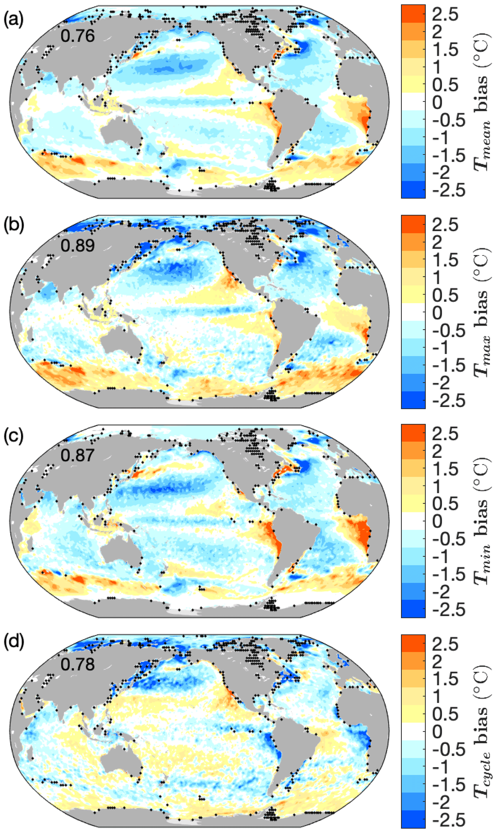
Figure 1Biases (model minus climatology) of multi-model mean in (a) Tmean, (b) Tmax, (c) Tmin and (d) Tcycle. Black dots mark grid points excluded from our analysis, as described in Sect. 2. The numbers indicate the global RMSE (∘C).
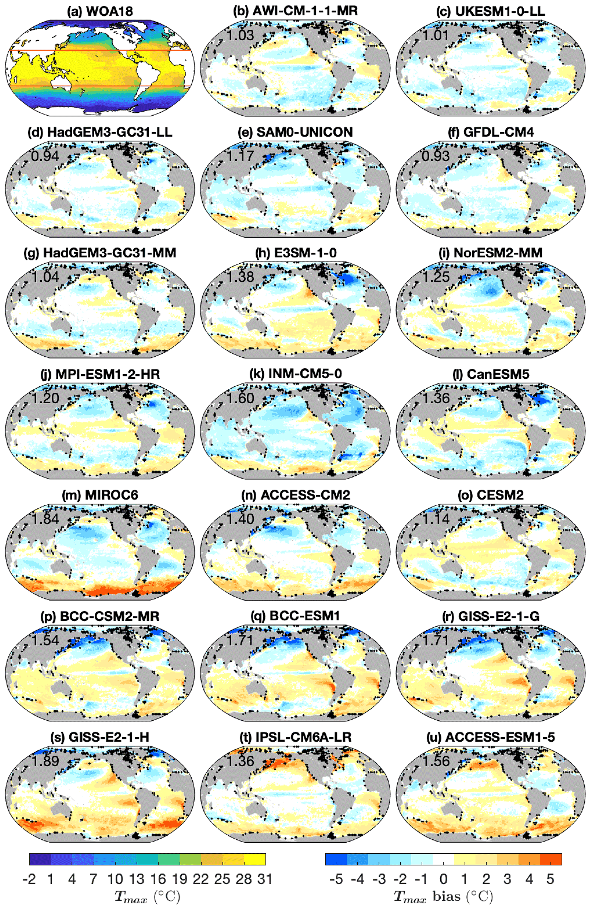
Figure 2(a) Tmax in WOA18 and (b–u) Tmax model biases. Black dots mark grid points excluded from our analysis, as described in Sect. 2. The numbers in (b–u) indicate the global RMSE of Tmax. Red lines in (a) are 30∘ N and 30∘ S. Note that the range of the bias colour bar is twice as much as in Fig. 1.
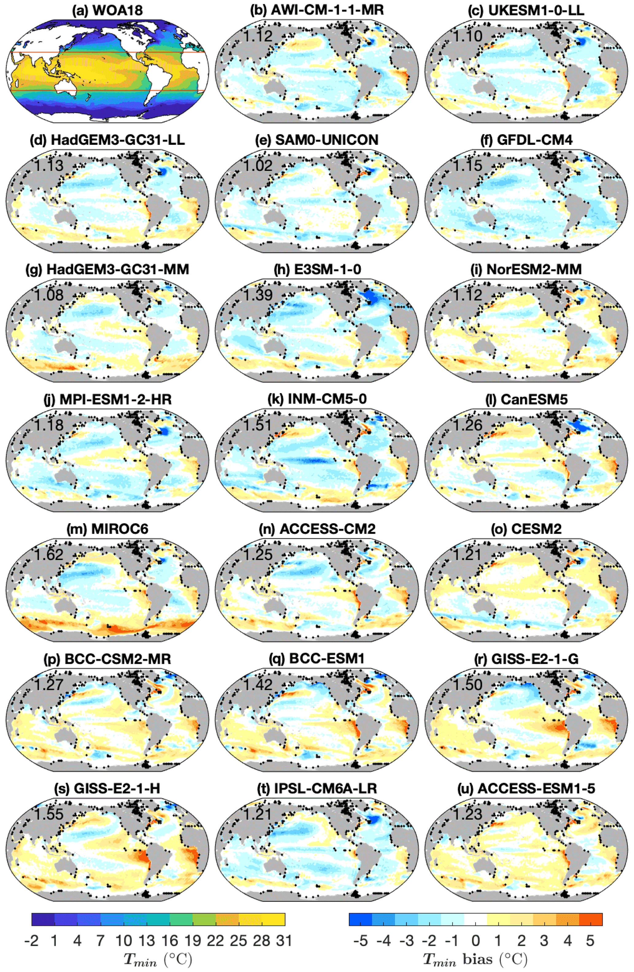
Figure 3As in Fig. 2 but for Tmin.
The magnitudes of biases in Tmax and Tmin vary from model to model (Figs. 2, 3 and 7). The multi-model mean has an RMSE of less than 1 ∘C in both Tmax and Tmin (0.89 and 0.87 ∘C, respectively). Most models have Tmax and Tmin RMSEs between 1 and 2 ∘C. Only HadGEM3-GC31-LL and GFDL-CM4 have a Tmax RMSE of less than 1 ∘C (0.94 and 0.93 ∘C, respectively). GISS-E2-1-H has the largest Tmax RMSE of 1.89 ∘C, and MIROC6 has the largest Tmin RMSE of 1.62 ∘C (Figs. 2 and 3). To test the dependence of the biases found on the realisation of models, we compared the first and second ensemble members (except for SAM0-UNICON and GFDL-CM4 as they have only one ensemble member). The differences between ensemble members are very small compared with the model biases (Figs. S1–S4 in the Supplement), and thus the model biases we report are robust.
In most of the models the global RMSE is larger in Tmax than in Tmin (Fig. 7a). As the bias in Tmax and Tmin is largely consistent with Tmean bias, the Tcycle RMSE is small compared to Tmax and Tmin RMSEs in most models. Different biases in Tmax, Tmin, Tcycle and Tmean suggest that models have different performances in simulating SST seasonal variation and annual mean. The “best” and “worst” models depend on whether you choose SST seasonal extrema or an annual mean as your metric. For example, GFDL-CM4 and HadGEM-GC31-MM have the smallest RMSE in Tmax, and thus they are best for simulating tropical cyclones and heatwaves; SAM0-UNICON has the smallest RMSE in Tmin, and thus it is best for simulating the properties of intermediate and deep waters.
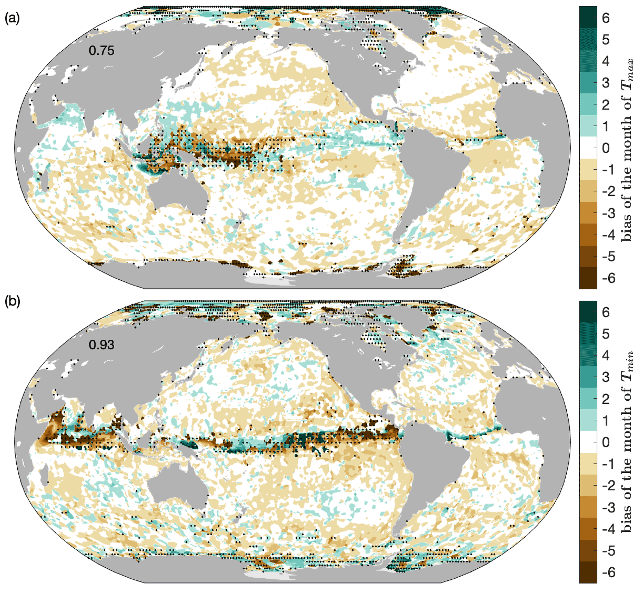
Figure 4Biases in the timing of (a) Tmax and (b) Tmin in the multi-model mean. Black dots mark grid points excluded from our analysis, as described in Sect. 2.
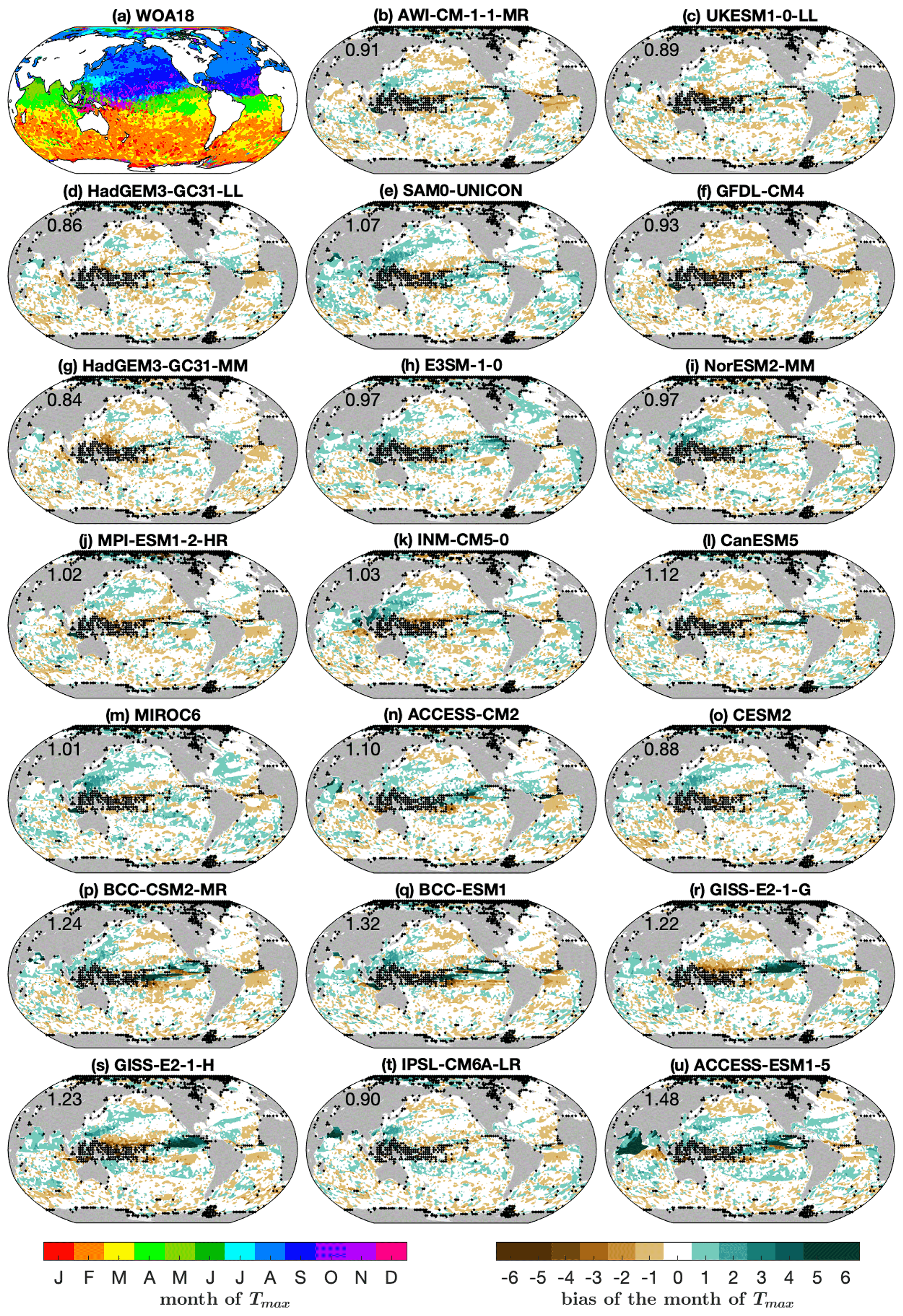
Figure 5(a) Timing of Tmax in WOA18 and (b–u) biases in the timing of Tmax in models. Black dots mark grid points excluded from our analysis, as described in Sect. 2.

Figure 6As in Fig. 5 but for the timing of Tmin.
The bias in the timing of Tmax and Tmin is within 1 month in most of the global ocean in most models (Figs. 4, 5 and 6). In the multi-model mean, Tmax and Tmin occur 1 month earlier than in WOA18 for most of the global ocean, whereas in some parts of the Arabian Sea and equatorial regions, they occur 1 month later (Fig. 4). The bias in the timing of Tmax and Tmin demonstrates that the seasonal cycles in CMIP6 models are out of phase with observations. In regions where monsoon prevails (e.g. the northwestern Indian Ocean), the timing bias suggests a bias in the onset of summer monsoon.
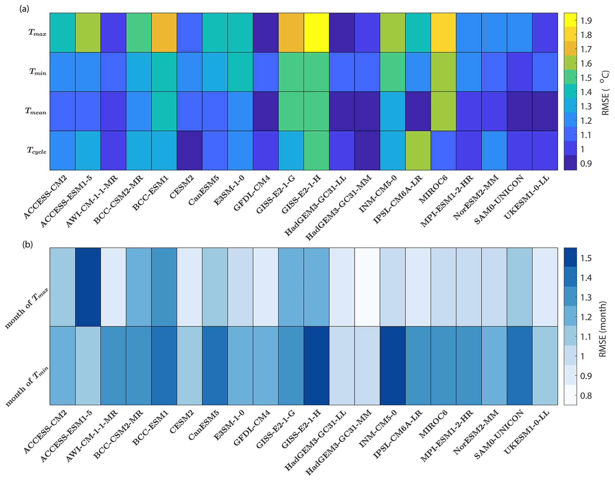
Figure 7The global area-weighted RMSE of the biases in (a) Tmax, Tmin, Tmean and Tcycle and (b) the timing of Tmax and Tmin.
Models have different performance in simulating the timing of Tmax and the timing of Tmin. All the models except ACCESS-ESM1-5 have a smaller global RMSE in the timing of Tmax than in the timing of Tmin (Fig. 7b). HadGEM3-GC31-MM has the smallest global RMSE in the timing of Tmax, whereas HadGEM3-GC31-LL and HadGEM3-GC31-MM have the smallest global RMSE in the timing of Tmin.
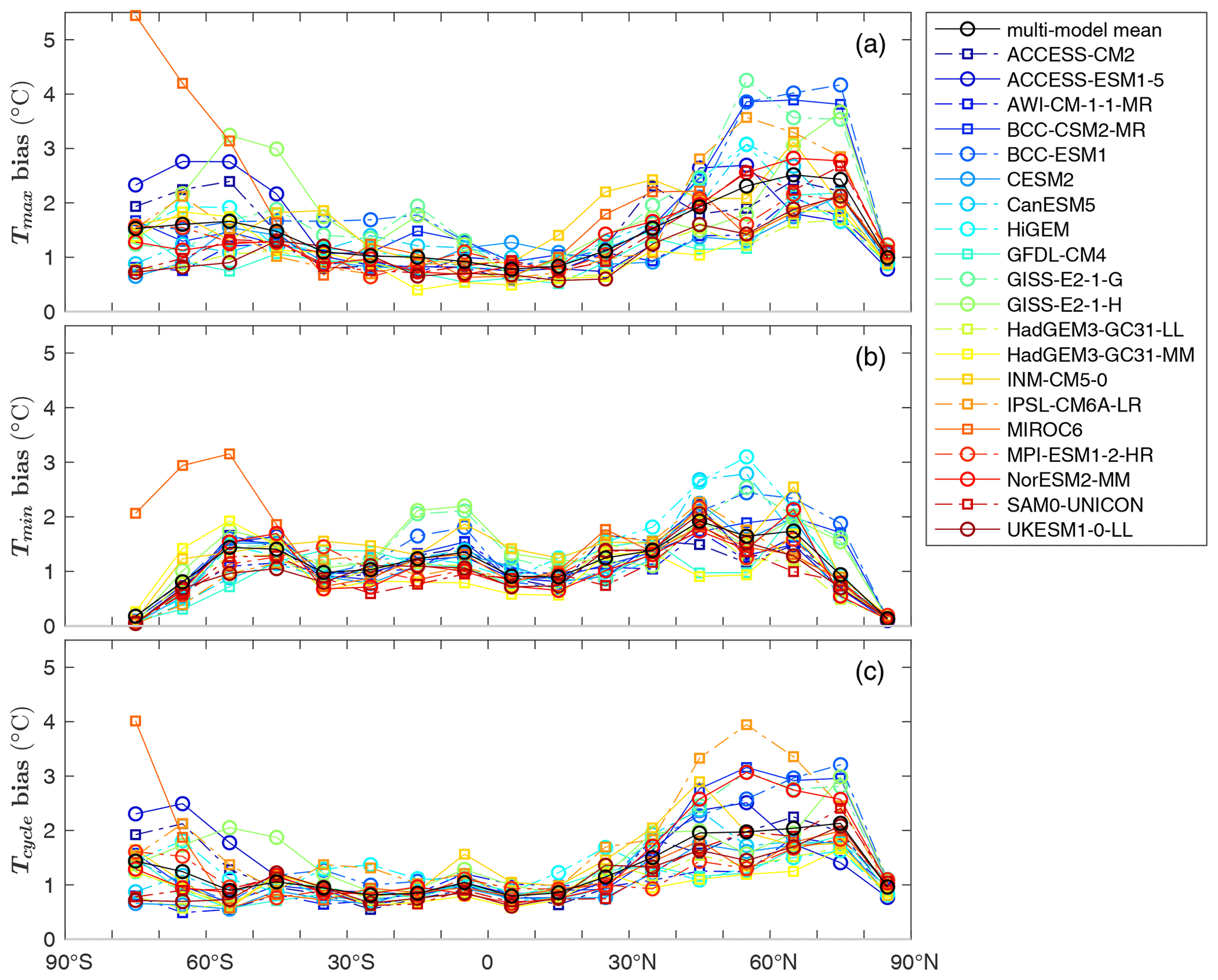
Tmax and Tmin biases vary with latitude (Figs. 1b, c, 2, 3 and 8a, b). High latitudes show larger biases than low latitudes. Typically, the RMSE of Tmax at 30–80∘ is 1–2 ∘C larger than at low latitudes (between 30∘ N and 30∘ S) (Fig. 8a). For GISS-E2-1-H, GISS-E2-1-G, BCC-CSM2-MR, BCC-ESM1 and IPSL-CM6A-LR, Tmax RMSEs at 30–80∘ N are about 3 ∘C larger than at low latitudes. A similar pattern is seen for Tmin, but the variation in biases with latitude is much smaller than for Tmax (Figs. 1c and 8b). Flato et al. (2013) found a similar result for some CMIP5 models, with larger zonal mean biases in Tmean between 30 and 70∘ than at other latitudes. The larger biases, and greater difference between Tmax and Tmin, at mid–high latitudes (greater than 30∘ in both hemispheres) may be explained by the large seasonal cycle of mixed-layer depth there. Shallower summer mixed layers have a smaller heat capacity; thus a small error in heat fluxes or mixing processes can result in a large bias for Tmax, though this will be modulated by any seasonal biases in mixed-layer depth. The larger inter-model biases in Tmax than in Tmin can be explained by the shallower mixed layer in summer, which can amplify SST biases due to biases in surface heat flux. The difference between biases in Tmax and Tmin leads to biases in Tcycle (Fig. 1d). The RMSE of Tcycle at low latitudes is typically 1 ∘C, whereas at mid–high latitudes it is larger, particularly in the Northern Hemisphere (Fig. 8c). The Tcycle RMSE in IPSL-CM6A-LR and MIROC6 reaches 4 ∘C at high latitudes (Fig. 8c).
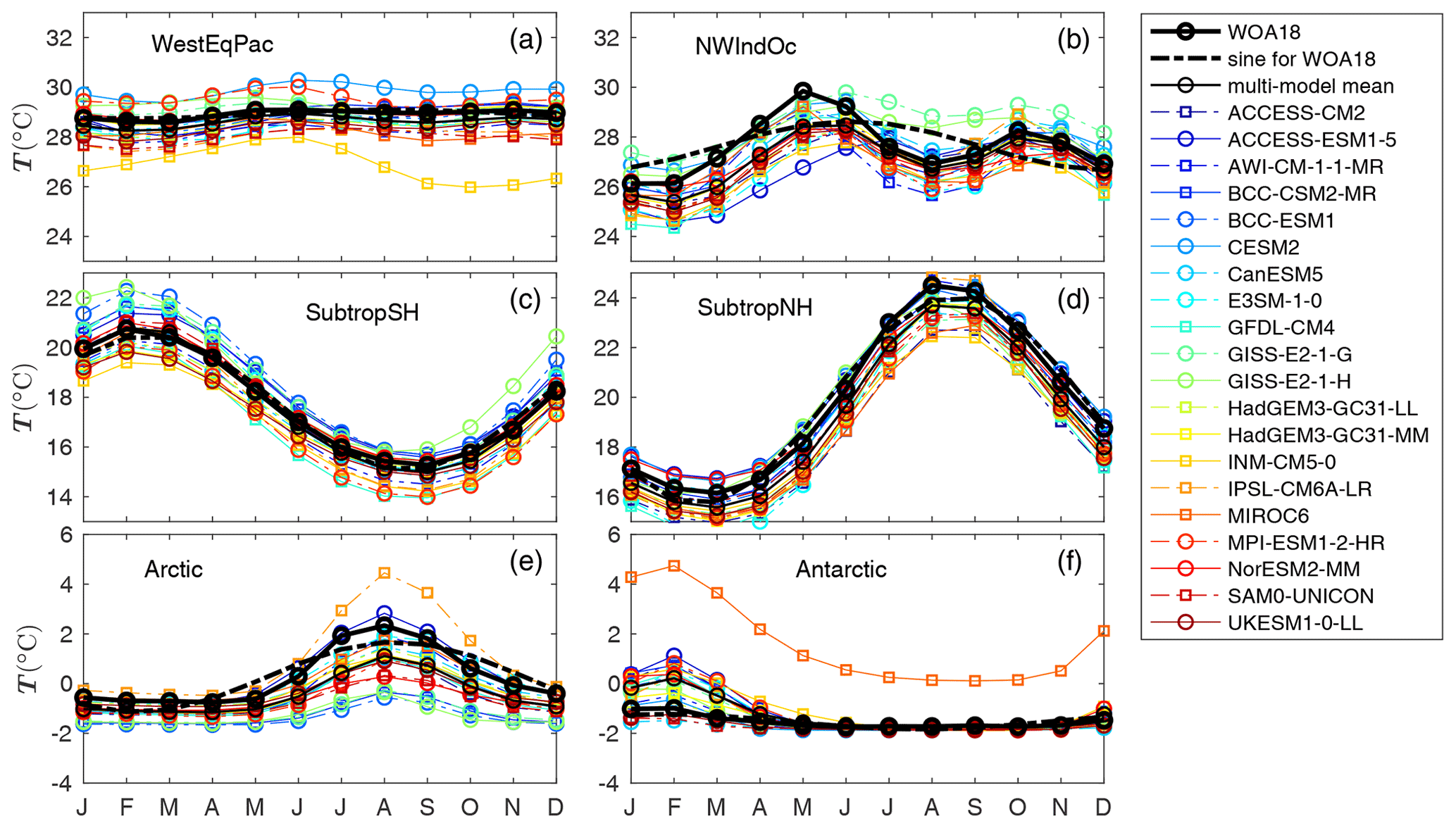
Figure 9Monthly time series of area-weighted mean SST over the (a) western equatorial Pacific (5∘ S–5∘ N, 140∘ E–160∘ W), (b) northwestern Indian Ocean (10–20∘ N, 60–70∘ E), (c) subtropical Southern Hemisphere (30–40∘ S), (d) subtropical Northern Hemisphere (30–40∘ N), (e) Arctic (70–80∘ N) and (f) Antarctic (70–80∘ S). The y-axis range is same for (a–f).
In polar regions, there are very small Tmin biases (Figs. 1c, 3 and 8b) except for MIROC6 in the Antarctic. Winter SSTs are close to freezing but cannot go below freezing because sea ice forms instead. If models have realistic freezing points, Tmin biases will be small. Some models have salinity-dependent freezing points (Beaumet et al., 2019), in which case a salinity bias could cause a bias in temperature. Tmin biases in the Arctic are larger than in the Antarctic (Figs. 1c and 9e, f), which suggests larger salinity biases in the Arctic.
In the subtropical North Pacific, the SST cold bias is typically 0.5–1 ∘C smaller in Tmax than Tmin, which leads to too large a Tcycle (Figs. 1b–d, 2 and 3). Zhu et al. (2020) showed a similar seasonal SST cold bias in the CMIP6 multi-model mean but not in the CMIP5 multi-model mean. Underestimated surface shortwave radiation and too strong westerly winds in the CMIP6 multi-model mean (Lyu et al., 2020; Li et al., 2020) are possible reasons for the year-round cold bias. The shortwave radiation bias is likely related to the bias of low-level cloud in the subtropics (Burls et al., 2017; Li and Xie, 2012), and its associated cold bias is smaller in winter when there is less solar radiation. The westerly winds cool the surface through latent heat flux and southward ocean advection due to Ekman transport. The latent heat loss shows a maximum in summer (Yu, 2007), while the ocean heat advection shows a maximum in winter when meridional SST gradients are greatest.
SST biases are seasonally dependent in the northeastern Pacific Inter Tropical Convergence Zone (ITCZ) (Figs. 1b, c, 2 and 3). For the multi-model mean, there is a warm bias in Tmax which exceeds 2 ∘C and a cold bias in Tmin of 0.5–1.5 ∘C. Similar seasonal biases exist in CMIP5 models and were linked to an easterly wind bias throughout the year there (Song and Zhang, 2020). A coarse atmospheric model resolution smooths out the elevation difference between mountains and oceans, which allows easterly trade winds to cross the mountains, leading to the easterly wind bias (Song and Zhang, 2020). An easterly bias of annual mean wind was found in the CMIP6 multi-model mean (Li et al., 2020; Lyu et al., 2020). If the easterly bias exists throughout the year, it can explain the seasonal SST bias we found. During winter–spring, the northeastern Pacific ITCZ is dominated by easterly winds, so overly strong easterly winds enhance surface evaporation and lead to cold biases. In contrast, during summer–autumn when westerly winds dominate, the simulated wind is too weak, which causes the warm bias. The northeastern Pacific is a region where tropical cyclones and heatwaves occur (Gilford et al., 2017; Frölicher and Laufkötter, 2018), so a warm bias of over 2 ∘C in Tmax may lead to the overprediction of tropical cyclones and heatwaves.
The multi-model mean has a cold bias in Tmax and a warm bias in Tmin over the northwest Pacific, leading to too small a Tcycle (bias of more than 2 ∘C) (Fig. 1b–d). The warm bias in winter can be seen in many models, especially in ACCESS-ESM1-5, BCC-ESM1, CanESM5 and INM-CM5-0 (Fig. 3). The winter warm bias east of Japan was also found in a CMIP5 multi-model mean (Wang et al., 2018), but from our results the warm bias extends further east (Fig. 1c).
The large cold biases at Northern Hemisphere high latitudes in BCC-CSM2-MR, BCC-ESM1, GISS-E2-1-G and GISS-E2-1-H are typically 2–5 ∘C smaller in Tmin than in Tmax (Figs. 2, 3 and 8a, b). These cold biases are likely to be linked to cloud biases due to the cooling radiative effect of low cloud (Myers et al., 2021). The negative cloud radiative forcing is excessive in BCC-CSM2-MR (Wu et al., 2019) and BCC-ESM1 (cloud simulation likely to be similar to BCC-CSM2-MR), while overestimated low-cloud cover in GISS-E2-1-G and GISS-E2-1-H (Kelley et al., 2020) blocks more of the incoming solar radiation. As solar radiation is negligible at high latitudes in winter, the SST cold bias due to cloud bias is much smaller in winter than in summer, consistent with our results. Deep winter mixed-layer depths and SSTs close to freezing likely also contribute to the smaller cold biases in Tmin than in Tmax at high latitudes.
In most models there is a warm Tmean bias in the Southern Ocean, commonly attributed to excessive shortwave radiation linked to cloud process representation deficiencies (Hyder et al., 2018). MIROC6 has an underestimated mid-level cloud cover (Tatebe et al., 2019); GISS-E2-1-G and GISS-E2-1-H have an underestimated shortwave cloud radiative forcing (Kelley et al., 2020), and hence they have pronounced warm biases in the Southern Ocean (Figs. 2, 3). The warm bias is larger for Tmax than Tmin (Figs. 1b, c, 2, 3 and 8a, b) because the lack of incoming solar radiation in winter means cloud biases have minimal effect on surface solar insolation. Shallower mixed-layer depths in summer will also tend to enhance any bias in incoming solar insolation. The larger warm bias in Tmax than Tmin results in a sea ice extent that is too small in most CMIP6 models, especially in summer (Beadling et al., 2020; Shu et al., 2020). As mode and intermediate waters primarily form within the winter mixed layer of the Antarctic Circumpolar Current (Talley, 1999), the Tmin warm bias can influence global ocean stratification.
MIROC6 stands out with the largest warm bias in the Southern Ocean (Figs. 2m and 3m), with a Tmax RMSE between 3 and 5 ∘C and Tmin RMSE between 2 and 3 ∘C at 50–80∘ S (Fig. 8a and b). The largest biases in MIROC6 occur in regions where there should be sea ice and where the deep ocean is ventilated. Beadling et al. (2020) found that MIROC6 has the lowest Southern Ocean sea ice extent among CMIP6 models in both summer and winter, and Tatebe et al. (2019) revealed annual warm biases exceeding 2 ∘C in the intermediate and deep layers of MIROC6.
In eastern boundary upwelling regions (especially the Benguela and Humboldt currents), most models have a seasonal warm bias that is 1–5 ∘C smaller in Tmax than Tmin (Figs. 1b, c, 2 and 3). Richter (2015) suggested that underestimation of stratocumulus cloud and insufficient upwelling due to overly weak winds contribute to the warm bias in eastern boundary upwelling regions. The warm bias we found therefore is likely associated with the underestimated surface shortwave radiation and overly weak, upwelling-favourable winds in CMIP6 models identified by Li et al. (2020). The warm bias may lead to excessive precipitation in the Atlantic Ocean off Angola and Namibia as shown by Rouault et al. (2003). Letelier et al. (2009) showed that in the Humboldt Current coastal region the cooling effect of upwelling is strongest in austral summer, which is consistent with the peak of upwelling-favourable wind in December and January. A poor simulation of the seasonal cloud and upwelling processes will contribute to the seasonality of SST biases in eastern boundary upwelling regions.
Most models have a seasonal warm SST bias in the eastern equatorial Atlantic (Figs. 1b, c, 2 and 3). The Tmin multi-model mean bias can be more than 2 ∘C larger than the Tmax multi-model mean bias. Richter and Tokinaga (2020) showed a similar seasonal warm bias in the CMIP6 multi-model mean, which is about 1–2 ∘C larger during June–July–August than March–April–May. Richter et al. (2012) argued that the warm SST bias in the eastern equatorial Atlantic during June–July–August is linked to overly deep thermoclines caused by overly weak easterlies during March–April–May. Therefore, the warm bias can be attributed to overly weak easterlies in the CMIP6 multi-model mean (Li et al., 2020; Lyu et al., 2020). GISS-E2-1-G and GISS-E2-1-H have the largest seasonality of SST warm bias in the eastern equatorial Atlantic, with Tmin biases up to 5 ∘C. Richter and Tokinaga (2020) illustrated that warmer than observed SSTs in the equatorial Atlantic lead to excessive precipitation. Roxy (2014) quantified the SST–precipitation relationship: a 1 ∘C SST increase corresponds to a 2 mm d−1 precipitation increase. Therefore, the 5 ∘C Tmin warm bias in GISS-E2-1-G and GISS-E2-1-H could cause a 10 mm d−1 increase in precipitation.
Although the amplitudes of biases are different in Tmax and Tmin, the global patterns and signs of Tmax and Tmin biases are similar to each other in most models (Figs. 2 and 3). Wang et al. (2014) indicated that the SST bias of the CMIP5 multi-model mean has a pattern independent of season but did not analyse the seasonality in bias in individual models. Our results show two exceptions: E3SM-1-0 and IPSL-CM6A-LR, which both have an overall warm bias in Tmax but an overall cold bias in Tmin (Figs. 2h, t and 3h, t), which tend to cancel out in the annual means. The Tmax RMSE is 1.38 ∘C for E3SM-1-0 and 1.36 ∘C for IPSL-CM6A-LR, and the Tmin RMSE is 1.39 ∘C for E3SM-1-0 and 1.21 ∘C for IPSL-CM6A-LR, whereas the Tmean RMSE is only 1.17 ∘C for E3SM-1-0 and 0.94 ∘C for IPSL-CM6A-LR. In E3SM-1-0, the global annual average mixed-layer depth is generally too shallow (Golaz et al., 2019), which can contribute to the summer SST warm bias and winter SST cold bias, and a similar process may be affecting IPSL-CM6A-LR. These results illustrate the risks involved in assessing only annual means, as models may have greater biases than assumed, so tropical cyclone formation, for example, may be overpredicted.
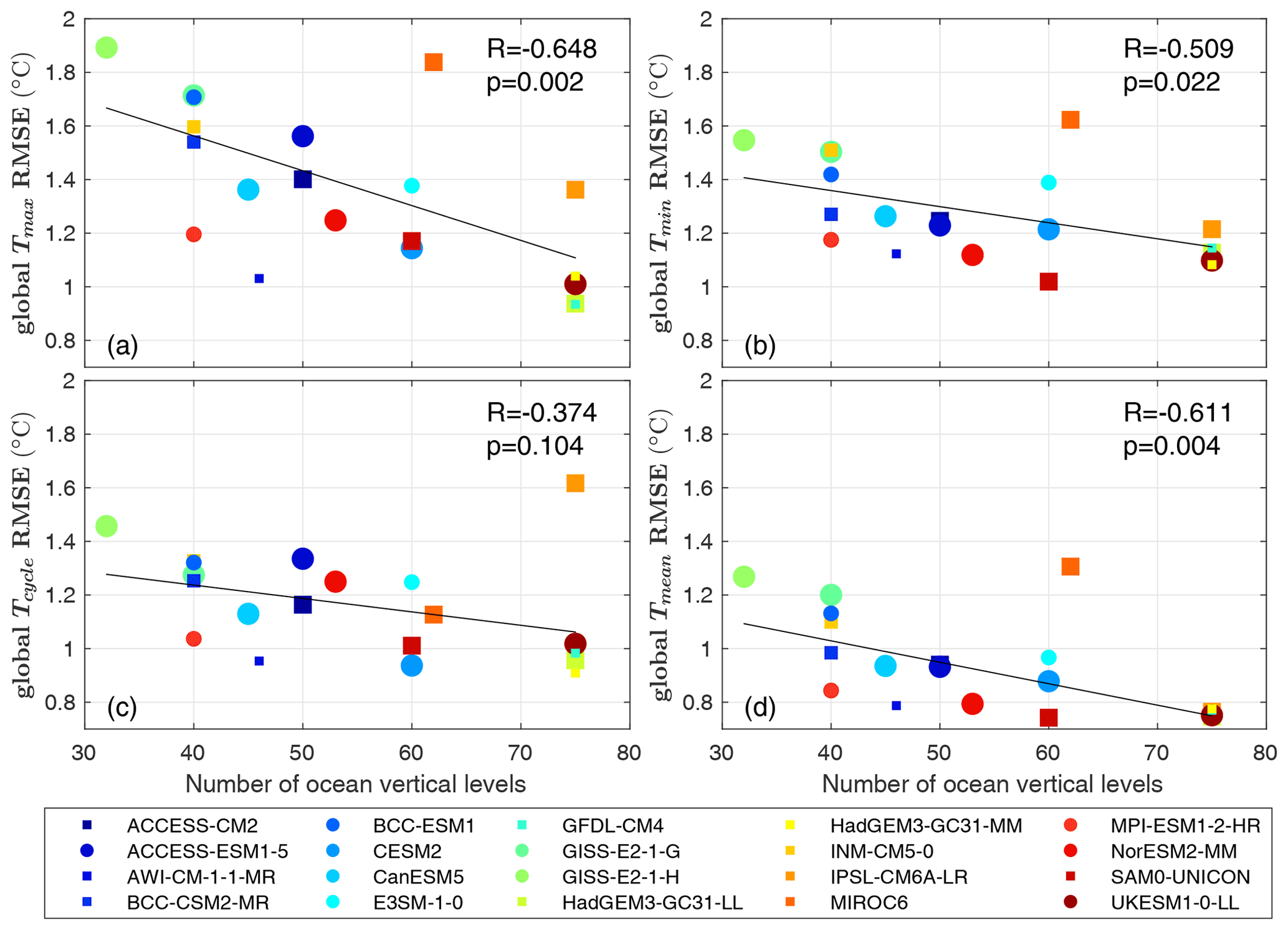
Figure 10Global RMSE of (a) Tmax, (b) Tmin, (c) Tcycle and (d) Tmean, all against the total number of vertical levels in the ocean. Circles represent earth system models, while squares represent non-earth system models. The size of the markers represents the ocean horizontal resolution for that model, with larger markers for models with lower horizontal resolution. The black line is the line of best fit (with the least sum of squared errors). The inter-model correlation R and p value are shown in each panel.
In midlatitudes the SST seasonal cycle is well represented by an annual sinusoid, whereas in equatorial and polar regions an annual sinusoid explains little of the total SST seasonal variance (Trenberth, 1983; Yashayaev and Zveryaev, 2001). In regions with fairly sinusoidal SST annual cycles such as the subtropics (sinusoidal signal explains 87 % of the observed variances in the subtropical Northern Hemisphere and 89 % of the observed variances in the subtropical Southern Hemisphere), models have realistic SST seasonal cycles with well-simulated amplitude and phase of the annual cycle (Fig. 9c and d). Phase biases are mainly within 1 month (Figs. 4, 5 and 6). In subtropical regions, seasonal SST biases are consistent with biases in Tmean. Differences between the Tmax and Tmin biases are smaller than those in non-sinusoidal regions (Fig. 9). In regions with non-sinusoidal SST seasonal cycles such as the western equatorial Pacific, northwestern Indian Ocean, the Arctic and the Antarctic (sinusoidal signal explains 33 %, 23 %, 58 % and 46 % of the observed variances), models tend to have biases in amplitudes or phases of their SST seasonal cycles (Figs. 4, 5, 6 and 9a–b, e–f).
In the western equatorial Pacific, the SST seasonal cycle in WOA18 is modest (less than 1 ∘C), whereas in some models such as MPI-ESM1-2-HR, GISS-E2-1-G, GISS-E2-1-H and especially INM-CM5-0, the seasonal cycle is much larger (Fig. 9a). In INM-CM5-0, the Tcycle is about 2 ∘C and there is a cold SST bias throughout the year, reaching 3 ∘C during September–October–November (Fig. 9a). Similar to our analysis, Volodin et al. (2017) noted that INM-CM5-0 has a cold bias of more than 4 ∘C in annual mean temperature in the upper 700 m of the western equatorial Pacific. The cold bias could limit the skills of models in simulations of the El Niño–Southern Oscillation (ENSO) and ENSO-induced teleconnections. For example, a cold bias in the western equatorial Pacific results in a rising branch of the Walker circulation that is too far west in many coupled climate models leading to too weak an ocean–atmosphere coupling and unrealistic ENSO dynamics (Bayr et al., 2018). The associated convective response along the Equator during ENSO events is too far west leading to a westward shift in the sea level pressure response in the North Pacific and precipitation response in the subtropics (Bayr et al., 2019).
In the northwestern Indian Ocean where the monsoon system prevails, SST has a semi-annual cycle, but most models are unable to reproduce this with the correct amplitude and phase (Figs. 4, 5, 6 and 9b). Most CMIP6 models have SST cold biases in this region throughout the year, while the biases are generally larger during March–April–May than other months and the multi-model mean fails to simulate the primary maximum SST (Fig. 9b). Cold SST biases in the northwestern Indian Ocean lead to a significant reduction in the monsoon rainfall over the Indian subcontinent (Prodhomme et al., 2014; Levine and Turner, 2012). Thus the cold biases in the CMIP6 models are likely to lead to overly weak monsoon precipitation. Consistent with our result, McKenna et al. (2020) found a cold SST bias over the northwestern Indian Ocean in the CMIP6 multi-model mean. Fathrio et al. (2017) showed that the SST cold bias over the western Indian Ocean in the CMIP5 multi-model mean has a seasonal cycle, with the coldest SST bias occurring in April, whereas the coldest SST bias in our CMIP6 multi-model mean occurs in May. GISS-E2-1-G and GISS-E2-1-H fail to simulate a realistic second minimum SST in August (Fig. 9b), which would lead to overly intense tropical cyclones. SST in the northwestern Indian Ocean determines the onset of the summer monsoon (Sijikumar and Rajeev, 2012; Jiang and Li, 2011). The primary maximum SST is 2 months later in ACCESS-ESM1-5 than in WOA18 (Fig. 9b), which suggests a delayed summer monsoon onset in projections using that model.
3.2 Impact of model characteristics on SST seasonal extrema
We have shown that biases in Tmax, Tmin and Tcycle are different between models. We now use the diversity in the 20 CMIP6 models to explore the effects of different model characteristics on the magnitude of these biases as quantified by global area-weighted RMSE for Tmax, Tmin, Tcycle and Tmean.
No significant correlation was found between the models' seasonal biases and horizontal ocean resolution (Fig. S5 in the Supplement). Chassignet et al. (2020) used four pairs of matched low-resolution and high-resolution ocean simulations from FSU-HYCOM, AWI-FESOM, NCAR-POP and IAP-LICOM to isolate the effect of ocean horizontal resolution and compared their representation of global SST. They found that enhanced horizontal resolution does not deliver unambiguous SST bias improvement in all regions for all models, which is consistent with our finding. Nor did we find any correlation of seasonal biases with atmospheric resolution (Figs. S6 and S7 in the Supplement), ocean grid type, ocean vertical coordinate and inclusion (or not) of biogeochemical processes (circles or squares in Figs. 10 and 11).
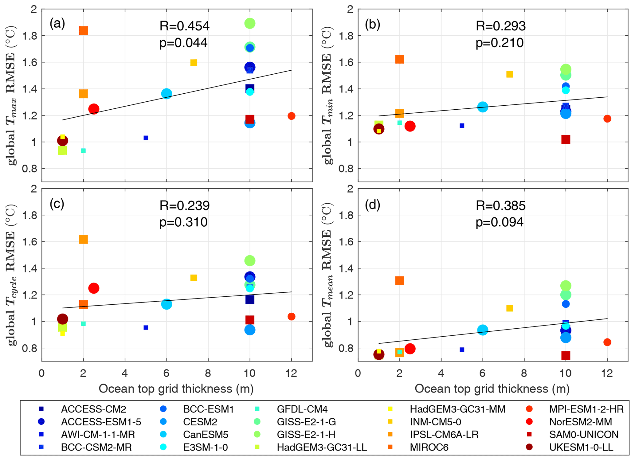
The only characteristic yielding a statistically significant relationship was the ocean vertical resolution (Figs. 10 and 11). The importance of vertical resolution for reducing seasonal biases is not unexpected: SST is influenced by ocean stratification and ocean vertical mixing processes, whose representation depends upon the vertical resolution. It has been found that high resolution in the upper ocean is important for the representation of diurnal and intraseasonal SST variability in ocean general circulation models (Misra et al., 2008; Xavier et al., 2008; Ge et al., 2017). Ideally we would have considered the number of vertical levels in the upper ocean. However, the number of vertical levels in the upper ocean (e.g. upper 200 m) cannot be unambiguously determined for models using an isopycnal or sigma vertical coordinate (6 out of 20 in our study) as their level depths vary with location and time (Bleck, 2002; Shchepetkin and McWilliams, 2005). Excluding the isopycnal and sigma models, the remaining high vertical-resolution models are mainly from the Met Office Hadley Centre family, and hence any relationship between SST biases and vertical resolution in the upper ocean might have been overly influenced by that particular family. Hence we use the total number of vertical levels and top grid cell thickness (Table 1) as proxies for the vertical resolution. Our study emphasises the importance of vertical resolution for simulating seasonal extreme SST and annual mean SST.
For the 20 models, there is a decrease in bias with increasing total number of vertical levels (Fig. 10). We calculated the inter-model correlation between global RMSE and the total number of vertical levels following the method of Wang et al. (2014). The relationship between SST biases and the total number of vertical levels is significant for Tmax, Tmin and Tmean (p values < 0.05), with the largest correlation of −0.648 for Tmax. The higher correlation between the global Tmax RMSE and ocean vertical resolution is likely linked to shallower mixed-layer depths in summer than in winter. RMSE is also correlated with top grid thickness (but with a smaller correlation than the total number of vertical levels): models with a smaller top grid thickness tend to have smaller biases (Fig. 11).
The impact of ocean vertical resolution on SST biases varies with latitude and season. Ocean vertical resolution is most important for Tmax at low latitudes (Figs. S8 and S9 in the Supplement). SST biases decrease with the number of vertical levels in the Benguela, Humboldt and California upwelling regions (Figs. S10–S12 in the Supplement). Only the Canary upwelling region, which has the smallest SST bias among the main four eastern boundary upwelling regions, does not have a good inter-model correlation between SST biases and ocean vertical resolution (Fig. S13 in the Supplement).
Using the newly released CMIP6 models, this study provides a global view of the biases in SST extrema, identifies regions with large seasonal bias and suggests a future direction to reduce these biases. To study the seasonal cycle of SST, we focus on Tmax and Tmin whenever they occur, rather than particular months. Global area-weighted Tmax, Tmin and Tcycle RMSEs are typically 1–2 ∘C. Most models have Tmax and Tmin biases of the same sign at most locations, apart from IPSL-CM6A-LR and E3SM-1-0, which have an overall warm bias in Tmax and an overall cold bias in Tmin. When averaged across the whole globe, the bias in Tmean is typically consistent with Tmax and Tmin biases, but certain regions (eastern boundary upwelling regions, polar regions, the eastern equatorial Atlantic, the North Pacific) show significant differences between winter and summer biases. The seasonal variation in the SST bias demonstrates the importance of evaluating model performance on Tmax and Tmin, not just Tmean. Seasonal processes related to wind and cloud could be the main reasons for seasonal SST biases but depend upon region. Further investigations of wind and cloud biases in CMIP6 models for different seasons could be undertaken to better understand the causes of seasonal SST biases. In regions with non-sinusoidal SST seasonal cycles, models tend to have biases in amplitudes and/or phases of their SST seasonal cycles. If there is a substantial change in the climate, it should be considered that the pattern of biases in Tmax and Tmin may change. For the models we examined, those with increased vertical resolution in the ocean generally had a better representation of SST extrema, particularly Tmax. This is likely related to the ability of the higher-resolution models to better represent the surface mixed layer and particularly shallow mixed layers in summer. For improving the accuracy of future climate projections, we suggest that as much priority (or possibly more) should be given to increasing vertical ocean model resolution as is given to increasing horizontal resolution.
All codes that support the finding of this study are available from Yanxin Wang, upon reasonable request.
The WOA18 climatology was obtained from https://www.ncei.noaa.gov/archive/accession/NCEI-WOA18/ (Boyer et al., 2018) on 14 August 2019. The WAGHC climatology was obtained from https://doi.org/10.1594/WDCC/WAGHC_V1.0 (Gouretski, 2018b) on 15 August 2019. HadISST was obtained from http://www.metoffice.gov.uk/hadobs/hadisst/ (Rayner et al., 2003) on 17 May 2019. CMIP6 data were obtained between 23 July 2020 and 31 July 2020 and can be freely downloaded from the Earth System Grid Federation (e.g. https://esgf-index1.ceda.ac.uk/ CMIP, 2022).
The supplement related to this article is available online at: https://doi.org/10.5194/os-18-839-2022-supplement.
YW performed data analysis and prepared the paper under the supervision of KJH, DPS and GMD.
The contact author has declared that neither they nor their co-authors have any competing interests.
Publisher's note: Copernicus Publications remains neutral with regard to jurisdictional claims in published maps and institutional affiliations.
We thank NOAA (National Oceanic and Atmospheric Administration), the University of Hamburg and the Met Office Hadley Centre for allowing access to the climatology data sets. We thank all modelling centres for carrying out the CMIP6 simulations used here and the Earth System Grid Federation (ESGF) for archiving the data and providing access. This work was supported by the European Research Council under the European Union's Horizon 2020 research and innovation programme (grant agreement no. 741120). YW was supported by the China Scholarship Council (grant agreement no. 201706310146). Computing and data storage resources were provided by JASMIN, the UK collaborative data analysis facility. We thank the anonymous reviewers for their comments and suggestions during the review of this paper.
This research has been supported by the China Scholarship Council (grant no. 201706310146) and the European Research Council, H2020 European Research Council (grant no. COMPASS (741120)).
This paper was edited by Anna Rubio and reviewed by two anonymous referees.
Andrews, M. B., Ridley, J. K., Wood, R. A., Andrews, T., Blockley, E. W., Booth, B., Burke, E., Dittus, A. J., Florek, P., and Gray, L. J.: Historical simulations with HadGEM3-GC3. 1 for CMIP6, J. Adv. Model. Earth Sy., 12, e2019MS001995, https://doi.org/10.1029/2019MS001995, 2020. a, b
Bayr, T., Latif, M., Dommenget, D., Wengel, C., Harlaß, J., and Park, W.: Mean-state dependence of ENSO atmospheric feedbacks in climate models, Clim. Dynam., 50, 3171–3194, https://doi.org/10.1007/s00382-017-3799-2, 2018. a
Bayr, T., Domeisen, D. I., and Wengel, C.: The effect of the equatorial Pacific cold SST bias on simulated ENSO teleconnections to the North Pacific and California, Clim. Dynam., 53, 3771–3789, https://doi.org/10.1007/s00382-019-04746-9, 2019. a
Beadling, R., Russell, J., Stouffer, R., Mazloff, M., Talley, L., Goodman, P., Sallée, J., Hewitt, H., Hyder, P., and Pandde, A.: Representation of Southern Ocean Properties across Coupled Model Intercomparison Project Generations: CMIP3 to CMIP6, J. Climate, 33, 6555–6581, https://doi.org/10.1175/JCLI-D-19-0970.1, 2020. a, b
Beaumet, J., Krinner, G., Déqué, M., Haarsma, R., and Li, L.: Assessing bias corrections of oceanic surface conditions for atmospheric models, Geosci. Model Dev., 12, 321–342, https://doi.org/10.5194/gmd-12-321-2019, 2019. a
Bi, D., Dix, M., Marsland, S., O'Farrell, S., Sullivan, A., Bodman, R., Law, R., Harman, I., Srbinovsky, J., Rashid, H. A., et al.: Configuration and spin-up of ACCESS-CM2, the new generation Australian Community Climate and Earth System Simulator Coupled Model, Journal of Southern Hemisphere Earth Systems Science, 70, 225–251, https://doi.org/10.1071/ES19040, 2020. a
Bleck, R.: An oceanic general circulation model framed in hybrid isopycnic-Cartesian coordinates, Ocean Model., 4, 55–88, https://doi.org/10.1016/S1463-5003(01)00012-9, 2002. a
Boucher, O., Servonnat, J., Albright, A. L., Aumont, O., Balkanski, Y., Bastrikov, V., Bekki, S., Bonnet, R., Bony, S., and Bopp, L.: Presentation and evaluation of the IPSL-CM6A-LR climate model, J. Adv. Model. Earth Sy., 12, e2019MS002010, https://doi.org/10.1029/2019ms002010, 2020. a
Boyer, T. P., Garcia, H. E., Locarnini, R. A., Zweng, M. M., Mishonov, A. V., Reagan, J. R., Weathers, K. A., Baranova, O. K., Seidov, D., and Smolyar, I. V.: World Ocean Atlas 2018. Temperature, NOAA National Centers for Environmental Information [data set], https://www.ncei.noaa.gov/archive/accession/NCEI-WOA18 (last access: 31 May 2022), 2018. a
Burls, N. J., Muir, L., Vincent, E. M., and Fedorov, A.: Extra-tropical origin of equatorial Pacific cold bias in climate models with links to cloud albedo, Clim. Dynam., 49, 2093–2113, https://doi.org/10.1007/s00382-016-3435-6, 2017. a
Chassignet, E. P., Yeager, S. G., Fox-Kemper, B., Bozec, A., Castruccio, F., Danabasoglu, G., Horvat, C., Kim, W. M., Koldunov, N., Li, Y., Lin, P., Liu, H., Sein, D. V., Sidorenko, D., Wang, Q., and Xu, X.: Impact of horizontal resolution on global ocean–sea ice model simulations based on the experimental protocols of the Ocean Model Intercomparison Project phase 2 (OMIP-2), Geosci. Model Dev., 13, 4595–4637, https://doi.org/10.5194/gmd-13-4595-2020, 2020. a
Cheung, W. W. and Frölicher, T. L.: Marine heatwaves exacerbate climate change impacts for fisheries in the northeast Pacific, Sci. Rep.-UK, 10, 1–10, https://doi.org/10.1038/s41598-020-63650-z, 2020. a
CMIP: Coupled Model Intercomparison Project Phase 6 (CMIP6) data, Working Group on Coupled Modeling of the World Climate Research Programme, Earth System Grid Federation [data set], https://esgf-index1.ceda.ac.uk/, last access: 1 June 2022. a
Danabasoglu, G., Lamarque, J.-F., Bacmeister, J., Bailey, D., DuVivier, A., Edwards, J., Emmons, L., Fasullo, J., Garcia, R., and Gettelman, A.: The Community Earth System Model version 2 (CESM2), J. Adv. Model. Earth Sy., 12, e2019MS001916, https://doi.org/10.1029/2019MS001916, 2020. a
Dare, R. A. and McBride, J. L.: The threshold sea surface temperature condition for tropical cyclogenesis, J. Climate, 24, 4570–4576, https://doi.org/10.1175/JCLI-D-10-05006.1, 2011. a
Fathrio, I., Iizuka, S., Manda, A., Kodama, Y.-M., Ishida, S., Moteki, Q., Yamada, H., and Tachibana, Y.: Assessment of western Indian Ocean SST bias of CMIP5 models, J. Geophys. Res.-Oceans, 122, 3123–3140, https://doi.org/10.1002/2016JC012443, 2017. a
Flato, G., Marotzke, J., Abiodun, B., Braconnot, P., Chou, S., Collins, W., Cox, P., Driouech, F., Emori, S., Eyring, V., Forest, C., Gleckler, P., Guilyardi, E., Jakob, C., Kattsov, V., Reason, C., and Rummukainen, M.: Evaluation of Climate Models, Climate Change 2013: The Physical Science Basis. Contribution of Working Group I to the Fifth Assessment Report of the Intergovernmental Panel on Climate Change, Cambridge University Press, Cambridge, United Kingdom and New York, NY, USA, 741–866, https://doi.org/10.1017/CBO9781107415324, 2013. a, b
Frölicher, T. L. and Laufkötter, C.: Emerging risks from marine heat waves, Nat. Commun., 9, 1–4, https://doi.org/10.1038/s41467-018-03163-6, 2018. a
Ge, X., Wang, W., Kumar, A., and Zhang, Y.: Importance of the vertical resolution in simulating SST diurnal and intraseasonal variability in an oceanic general circulation model, J. Climate, 30, 3963–3978, https://doi.org/10.1175/JCLI-D-16-0689.1, 2017. a
Gilford, D. M., Solomon, S., and Emanuel, K. A.: On the seasonal cycles of tropical cyclone potential intensity, J. Climate, 30, 6085–6096, https://doi.org/10.1175/JCLI-D-16-0827.1, 2017. a
Golaz, J.-C., Caldwell, P. M., Van Roekel, L. P., Petersen, M. R., Tang, Q., Wolfe, J. D., Abeshu, G., Anantharaj, V., Asay-Davis, X. S., and Bader, D. C.: The DOE E3SM coupled model version 1: Overview and evaluation at standard resolution, J. Adv. Model. Earth Sy., 11, 2089–2129, https://doi.org/10.1029/2018MS001603, 2019. a, b
Gouretski, V.: World Ocean Circulation Experiment – Argo Global Hydrographic Climatology, Ocean Sci., 14, 1127–1146, https://doi.org/10.5194/os-14-1127-2018, 2018a. a
Gouretski, V.: WOCE-Argo Global Hydrographic Climatology (WAGHC Version 1.0), World Data Center for Climate (WDCC) at DKRZ [data set], https://doi.org/10.1594/WDCC/WAGHC_V1.0, 2018b. a
Held, I., Guo, H., Adcroft, A., Dunne, J., Horowitz, L., Krasting, J., Shevliakova, E., Winton, M., Zhao, M., and Bushuk, M.: Structure and performance of GFDL's CM4. 0 climate model, J. Adv. Model. Earth Sy., 11, 3691–3727, https://doi.org/10.1029/2019MS001829, 2019. a
Holland, G. J.: The maximum potential intensity of tropical cyclones, J. Atmos. Sci., 54, 2519–2541, https://doi.org/10.1175/1520-0469(1997)054%3C2519:TMPIOT%3E2.0.CO;2, 1997. a
Hughes, T. P., Anderson, K. D., Connolly, S. R., Heron, S. F., Kerry, J. T., Lough, J. M., Baird, A. H., Baum, J. K., Berumen, M. L., Bridge, T. C., et al.: Spatial and temporal patterns of mass bleaching of corals in the Anthropocene, Science, 359, 80–83, https://doi.org/10.1126/science.aan8048, 2018. a
Hyder, P., Edwards, J. M., Allan, R. P., Hewitt, H. T., Bracegirdle, T. J., Gregory, J. M., Wood, R. A., Meijers, A. J., Mulcahy, J., and Field, P.: Critical Southern Ocean climate model biases traced to atmospheric model cloud errors, Nat. Commun., 9, 1–17, https://doi.org/10.1038/s41467-018-05634-2, 2018. a
Jiang, X. and Li, J.: Influence of the annual cycle of sea surface temperature on the monsoon onset, J. Geophys. Res-Atmos., 116, D10105, https://doi.org/10.1029/2010JD015236, 2011. a
Jones, T., Parrish, J. K., Peterson, W. T., Bjorkstedt, E. P., Bond, N. A., Ballance, L. T., Bowes, V., Hipfner, J. M., Burgess, H. K., Dolliver, J. E., et al.: Massive mortality of a planktivorous seabird in response to a marine heatwave, Geophys. Res. Lett., 45, 3193–3202, https://doi.org/10.1002/2017GL076164, 2018. a
Kelley, M., Schmidt, G. A., Nazarenko, L. S., Bauer, S. E., Ruedy, R., Russell, G. L., Ackerman, A. S., Aleinov, I., Bauer, M., and Bleck, R.: GISS-E2. 1: Configurations and Climatology, J. Adv. Model. Earth Sy., 12, e2019MS002025, https://doi.org/10.1029/2019MS002025, 2020. a, b, c, d
Law, R. M., Ziehn, T., Matear, R. J., Lenton, A., Chamberlain, M. A., Stevens, L. E., Wang, Y.-P., Srbinovsky, J., Bi, D., Yan, H., and Vohralik, P. F.: The carbon cycle in the Australian Community Climate and Earth System Simulator (ACCESS-ESM1) – Part 1: Model description and pre-industrial simulation, Geosci. Model Dev., 10, 2567–2590, https://doi.org/10.5194/gmd-10-2567-2017, 2017. a
Letelier, J., Pizarro, O., and Nuñez, S.: Seasonal variability of coastal upwelling and the upwelling front off central Chile, J. Geophys. Res.-Oceans, 114, C12009, https://doi.org/10.1029/2008JC005171, 2009. a
Levine, R. C. and Turner, A. G.: Dependence of Indian monsoon rainfall on moisture fluxes across the Arabian Sea and the impact of coupled model sea surface temperature biases, Clim. Dynam., 38, 2167–2190, https://doi.org/10.1007/s00382-011-1096-z, 2012. a
Li, G. and Xie, S.-P.: Origins of tropical-wide SST biases in CMIP multi-model ensembles, Geophys. Res. Lett., 39, L22703, https://doi.org/10.1029/2012gl053777, 2012. a
Li, J.-L., Xu, K.-M., Jiang, J., Lee, W.-L., Wang, L.-C., Yu, J.-Y., Stephens, G., Fetzer, E., and Wang, Y.-H.: An overview of CMIP5 and CMIP6 simulated cloud ice, radiation fields, surface wind stress, sea surface temperatures, and precipitation over tropical and subtropical oceans, J. Geophys. Res-Atmos., 125, e2020JD032848, https://doi.org/10.1029/2020JD032848, 2020. a, b, c, d
Liu, F., Lu, J., Luo, Y., Huang, Y., and Song, F.: On the oceanic origin for the enhanced seasonal cycle of SST in the midlatitudes under global warming, J. Climate, 33, 8401–8413, https://doi.org/10.1175/JCLI-D-20-0114.1, 2020. a
Locarnini, R. A., Mishonov, A. V., Baranova, O. K., Boyer, T. P., Zweng, M. M., Garcia, H. E., Reagan, J. R., Seidov, D., Weathers, K., Paver, C. R., and Smolyar, I.: World Ocean Atlas 2018, Volume 1: Temperature, US government Printing Office, Washington, DC, 2018. a
Lyu, K., Zhang, X., and Church, J. A.: Regional dynamic sea level simulated in the CMIP5 and CMIP6 models: mean biases, future projections, and their linkages, J. Climate, 33, 6377–6398, https://doi.org/10.1175/JCLI-D-19-1029.1, 2020. a, b, c
McKenna, S., Santoso, A., Gupta, A. S., Taschetto, A. S., and Cai, W.: Indian Ocean Dipole in CMIP5 and CMIP6: characteristics, biases, and links to ENSO, Sci. Rep.-UK, 10, 1–13, https://doi.org/10.1038/s41598-020-68268-9, 2020. a
Misra, V., Marx, L., Brunke, M., and Zeng, X.: The equatorial Pacific cold tongue bias in a coupled climate model, J. Climate, 21, 5852–5869, https://doi.org/10.1175/2008JCLI2205.1, 2008. a
Müller, W. A., Jungclaus, J. H., Mauritsen, T., Baehr, J., Bittner, M., Budich, R., Bunzel, F., Esch, M., Ghosh, R., and Haak, H.: A Higher-resolution Version of the Max Planck Institute Earth System Model (MPI-ESM1. 2-HR), J. Adv. Model. Earth Sy., 10, 1383–1413, https://doi.org/10.1029/2017MS001217, 2018. a
Myers, T. A., Scott, R. C., Zelinka, M. D., Klein, S. A., Norris, J. R., and Caldwell, P. M.: Observational constraints on low cloud feedback reduce uncertainty of climate sensitivity, Nat. Clim. Change, 11, 501–507, https://doi.org/10.1038/s41558-021-01039-0, 2021. a
Palmen, E.: On the formation and structure of tropical hurricanes, Geophysica, 3, 26–38, 1948. a
Park, S., Shin, J., Kim, S., Oh, E., and Kim, Y.: Global climate simulated by the Seoul National University atmosphere model version 0 with a unified convection scheme (SAM0-UNICON), J. Climate, 32, 2917–2949, https://doi.org/10.1175/JCLI-D-18-0796.1, 2019. a
Prodhomme, C., Terray, P., Masson, S., Izumo, T., Tozuka, T., and Yamagata, T.: Impacts of Indian Ocean SST biases on the Indian Monsoon: as simulated in a global coupled model, Clim. Dynam., 42, 271–290, https://doi.org/10.1007/s00382-013-1671-6, 2014. a
Prodhomme, C., Voldoire, A., Exarchou, E., Deppenmeier, A.-L., García-Serrano, J., and Guemas, V.: How does the seasonal cycle control equatorial Atlantic interannual variability?, Geophys. Res. Lett., 46, 916–922, https://doi.org/10.1029/2018GL080837, 2019. a
Rayner, N., Parker, D. E., Horton, E., Folland, C. K., Alexander, L. V., Rowell, D., Kent, E., and Kaplan, A.: Global analyses of sea surface temperature, sea ice, and night marine air temperature since the late nineteenth century, J. Geophys. Res-Atmos., 108, https://doi.org/10.1029/2002jd002670, 2003 (data available at: http://www.metoffice.gov.uk/hadobs/hadisst/, last access: 1 June 2022). a, b
Richter, I.: Climate model biases in the eastern tropical oceans: causes, impacts and ways forward, WIREs Clim. Change, 6, 345–358, https://doi.org/10.1002/wcc.338, 2015. a
Richter, I. and Tokinaga, H.: An overview of the performance of CMIP6 models in the tropical Atlantic: mean state, variability, and remote impacts, Clim. Dynam., 55, 2579–2601, https://doi.org/10.1007/s00382-020-05409-w, 2020. a, b, c, d
Richter, I., Xie, S.-P., Wittenberg, A. T., and Masumoto, Y.: Tropical Atlantic biases and their relation to surface wind stress and terrestrial precipitation, Clim. Dynam., 38, 985–1001, https://doi.org/10.1007/s00382-011-1038-9, 2012. a, b
Richter, I., Xie, S.-P., Behera, S. K., Doi, T., and Masumoto, Y.: Equatorial Atlantic variability and its relation to mean state biases in CMIP5, Clim. Dynam., 42, 171–188, https://doi.org/10.1007/s00382-012-1624-5, 2014. a
Rouault, M., Florenchie, P., Fauchereau, N., and Reason, C. J.: South East tropical Atlantic warm events and southern African rainfall, Geophys. Res. Lett., 30, GL014840, https://doi.org/10.1029/2002GL014840, 2003. a
Roxy, M.: Sensitivity of precipitation to sea surface temperature over the tropical summer monsoon region–and its quantification, Clim. Dynam., 43, 1159–1169, https://doi.org/10.1007/s00382-013-1881-y, 2014. a
Seland, Ø., Bentsen, M., Olivié, D., Toniazzo, T., Gjermundsen, A., Graff, L. S., Debernard, J. B., Gupta, A. K., He, Y.-C., Kirkevåg, A., Schwinger, J., Tjiputra, J., Aas, K. S., Bethke, I., Fan, Y., Griesfeller, J., Grini, A., Guo, C., Ilicak, M., Karset, I. H. H., Landgren, O., Liakka, J., Moseid, K. O., Nummelin, A., Spensberger, C., Tang, H., Zhang, Z., Heinze, C., Iversen, T., and Schulz, M.: Overview of the Norwegian Earth System Model (NorESM2) and key climate response of CMIP6 DECK, historical, and scenario simulations, Geosci. Model Dev., 13, 6165–6200, https://doi.org/10.5194/gmd-13-6165-2020, 2020. a
Sellar, A. A., Jones, C. G., Mulcahy, J. P., Tang, Y., Yool, A., Wiltshire, A., O'Connor, F. M., Stringer, M., Hill, R., and Palmieri, J.: UKESM1: Description and evaluation of the UK Earth System Model, J. Adv. Model. Earth Sy., 11, 4513–4558, https://doi.org/10.1029/2019MS001739, 2019. a
Semmler, T., Danilov, S., Gierz, P., Goessling, H., Hegewald, J., Hinrichs, C., Koldunov, N. V., Khosravi, N., Mu, L., and Rackow, T.: Simulations for CMIP6 with the AWI climate model AWI-CM-1-1, J. Adv. Model. Earth Sy., 12, e2019MS002009, https://doi.org/10.1029/2019MS002009, 2020. a
Shchepetkin, A. F. and McWilliams, J. C.: The regional oceanic modeling system (ROMS): a split-explicit, free-surface, topography-following-coordinate oceanic model, Ocean Model., 9, 347–404, https://doi.org/10.1016/j.ocemod.2004.08.002, 2005. a
Shu, Q., Wang, Q., Song, Z., Qiao, F., Zhao, J., Chu, M., and Li, X.: Assessment of sea ice extent in CMIP6 with comparison to observations and CMIP5, Geophys. Res. Lett., 47, e2020GL087965, https://doi.org/10.1029/2020GL087965, 2020. a
Sijikumar, S. and Rajeev, K.: Role of the Arabian Sea warm pool on the precipitation characteristics during the monsoon onset period, J. Climate, 25, 1890–1899, https://doi.org/10.1175/JCLI-D-11-00286.1, 2012. a
Song, F. and Zhang, G. J.: The impacts of horizontal resolution on the seasonally dependent biases of the Northeastern Pacific ITCZ in coupled climate models, J. Climate, 33, 941–957, https://doi.org/10.1175/JCLI-D-19-0399.1, 2020. a, b, c
Sun, Y., Zhong, Z., Li, T., Yi, L., Hu, Y., Wan, H., Chen, H., Liao, Q., Ma, C., and Li, Q.: Impact of ocean warming on tropical cyclone size and its destructiveness, Sci. Rep.-UK, 7, 1–10, https://doi.org/10.1038/s41598-017-08533-6, 2017. a
Swart, N. C., Cole, J. N. S., Kharin, V. V., Lazare, M., Scinocca, J. F., Gillett, N. P., Anstey, J., Arora, V., Christian, J. R., Hanna, S., Jiao, Y., Lee, W. G., Majaess, F., Saenko, O. A., Seiler, C., Seinen, C., Shao, A., Sigmond, M., Solheim, L., von Salzen, K., Yang, D., and Winter, B.: The Canadian Earth System Model version 5 (CanESM5.0.3), Geosci. Model Dev., 12, 4823–4873, https://doi.org/10.5194/gmd-12-4823-2019, 2019. a
Talley, L. D.: Some aspects of ocean heat transport by the shallow, intermediate and deep overturning circulations, Geophysical Monograph-American Geophysical Union, Washington, DC, 112, 1–22, 1999. a
Tatebe, H., Ogura, T., Nitta, T., Komuro, Y., Ogochi, K., Takemura, T., Sudo, K., Sekiguchi, M., Abe, M., Saito, F., Chikira, M., Watanabe, S., Mori, M., Hirota, N., Kawatani, Y., Mochizuki, T., Yoshimura, K., Takata, K., O'ishi, R., Yamazaki, D., Suzuki, T., Kurogi, M., Kataoka, T., Watanabe, M., and Kimoto, M.: Description and basic evaluation of simulated mean state, internal variability, and climate sensitivity in MIROC6, Geosci. Model Dev., 12, 2727–2765, https://doi.org/10.5194/gmd-12-2727-2019, 2019. a, b, c
Trenberth, K. E.: What are the seasons?, B. Am. Meteorol. Soc., 64, 1276–1282, https://doi.org/10.1175/1520-0477(1983)064<1276:WATS>2.0.CO;2, 1983. a
Volodin, E., Mortikov, E., Kostrykin, S., Galin, V. Y., Lykossov, V., Gritsun, A., Diansky, N., Gusev, A., and Iakovlev, N.: Simulation of the present-day climate with the climate model INMCM5, Clim. Dynam., 49, 3715–3734, https://doi.org/10.1007/s00382-017-3539-7, 2017. a, b
Wang, C., Zhang, L., Lee, S.-K., Wu, L., and Mechoso, C. R.: A global perspective on CMIP5 climate model biases, Nat. Clim. Change, 4, 201–205, https://doi.org/10.1038/nclimate2118, 2014. a, b, c, d
Wang, C., Zou, L., and Zhou, T.: SST biases over the Northwest Pacific and possible causes in CMIP5 models, Science China Earth Sciences, 61, 792–803, https://doi.org/10.1007/s11430-017-9171-8, 2018. a
Wu, T., Lu, Y., Fang, Y., Xin, X., Li, L., Li, W., Jie, W., Zhang, J., Liu, Y., Zhang, L., Zhang, F., Zhang, Y., Wu, F., Li, J., Chu, M., Wang, Z., Shi, X., Liu, X., Wei, M., Huang, A., Zhang, Y., and Liu, X.: The Beijing Climate Center Climate System Model (BCC-CSM): the main progress from CMIP5 to CMIP6 , Geosci. Model Dev., 12, 1573–1600, https://doi.org/10.5194/gmd-12-1573-2019, 2019. a, b
Wu, T., Zhang, F., Zhang, J., Jie, W., Zhang, Y., Wu, F., Li, L., Yan, J., Liu, X., Lu, X., Tan, H., Zhang, L., Wang, J., and Hu, A.: Beijing Climate Center Earth System Model version 1 (BCC-ESM1): model description and evaluation of aerosol simulations, Geosci. Model Dev., 13, 977–1005, https://doi.org/10.5194/gmd-13-977-2020, 2020. a
Xavier, P. K., Duvel, J.-P., and Doblas-Reyes, F. J.: Boreal summer intraseasonal variability in coupled seasonal hindcasts, J. Climate, 21, 4477–4497, https://doi.org/10.1175/2008JCLI2216.1, 2008. a
Yashayaev, I. M. and Zveryaev, I. I.: Climate of the seasonal cycle in the North Pacific and the North Atlantic oceans, Int. J. Climatol., 21, 401–417, https://doi.org/10.1002/joc.585, 2001. a
Yu, L.: Global variations in oceanic evaporation (1958–2005): The role of the changing wind speed, J. Climate, 20, 5376–5390, https://doi.org/10.1175/2007JCLI1714.1, 2007. a
Zhang, L. and Zhao, C.: Processes and mechanisms for the model SST biases in the North Atlantic and North Pacific: a link with the Atlantic meridional overturning circulation, J. Adv. Model. Earth Sy., 7, 739–758, https://doi.org/10.1002/2014MS000415, 2015. a
Zhu, Y., Zhang, R.-H., and Sun, J.: North Pacific upper-ocean cold temperature biases in CMIP6 simulations and the role of regional vertical mixing, J. Climate, 33, 7523–7538, https://doi.org/10.1175/jcli-d-19-0654.1, 2020. a, b