Tracer and observationally derived constraints on diapycnal diffusivities in an ocean state estimate

Use of an ocean parameter and state estimation framework – such as the Estimating the Circulation and Climate of the Ocean (ECCO) framework – could provide an opportunity to learn about the spatial distribution of the diapycnal diffusivity parameter (κ_ρ) that observations alone cannot due to gaps in coverage. However, we show that the inclusion of misfits to observed physical variables – such as in situ temperature, salinity, and pressure – currently accounted for in ECCO is not sufficient, as κ_ρ from ECCO does not agree closely with any observationally derived product. These observationally derived κ_ρ products were inferred from microstructure measurements, derived from Argo and conductivity–temperature–depth (CTD) data using a strain-based parameterization of fine-scale hydrographic structure, or calculated from climatological and seafloor data using a parameterization of tidal mixing. The κ_ρ products are in close agreement with one another but have both measurement and structural uncertainties, whereas tracers can have relatively small measurement uncertainties. With the ultimate goal being to jointly improve the ECCO state estimate and representation of κ_ρ in ECCO, we investigate whether adjustments in κ_ρ due to inclusion of misfits to a tracer – dissolved oxygen concentrations from an annual climatology – would be similar to those due to inclusion of misfits to observationally derived κ_ρ products. We do this by performing sensitivity analyses with ECCO. We compare multiple adjoint sensitivity calculations: one configuration uses misfits to observationally derived κ_ρ, and the other uses misfits to observed dissolved oxygen concentrations. We show that adjoint sensitivities of dissolved oxygen concentration misfits to the state estimate's control space typically direct κ_ρ to improve relative to the observationally derived values. These results suggest that the inclusion of oxygen in ECCO's misfits will improve κ_ρ in ECCO, particularly in (sub)tropical regions.

1 Introduction

We consider the challenges with using observational data in the context of a parameter and state estimation framework to infer the global distribution of ocean mixing. Ocean models must parameterize the unresolved, turbulent diffusion of oceanic tracers. Ocean mixing is typically conceptualized in terms of diffusion along and across isopycnal surfaces. Subgrid-scale transport of isopycnal thickness (or bolus) – which is effectively an advective contribution to tracer budgets – must also be parameterized. Ocean models often represent these unresolved processes with three parameters: the across-isopycnal mixing parameter (diapycnal diffusivity; Munk and Wunsch, 1998), the along-isopycnal mixing parameter (Redi coefficient; Redi, 1982), and the eddy isopycnal thickness transport parameter (Gent–McWilliams coefficient; Gent and McWilliams, 1990). Diapycnal mixing is an essential component in explaining the observed oceanic stratification (Munk and Wunsch, 1998; Gnanadesikan, 1999; Scott and Marotzke, 2002). Changes in the background diapycnal diffusivity (Dalan et al., 2005; Krasting et al., 2018; Hieronymus et al., 2019; Sinha et al., 2020), Redi coefficient (Gnanadesikan et al., 2015; Ehlert et al., 2017), and Gent–McWilliams coefficient (Danabasoglu and McWilliams, 1995) are known to have a profound influence on climate simulations through alterations in the response to surface flux perturbations and changes in ventilation rates.

The spatiotemporal variabilities suggested in previous studies of the Redi coefficient (Abernathey and Marshall, 2013; Bates et al., 2014; Forget et al., 2015b; Cole et al., 2015; Busecke and Abernathey, 2019; Groeskamp et al., 2020) and Gent–McWilliams coefficient (Forget et al., 2015b; Katsumata, 2016; Bachman et al., 2020) fields are virtually absent in ocean models. There is also a dearth of independent observations with which to assess their observationally derived values (Cole et al., 2015; Katsumata, 2016; Roach et al., 2018; Groeskamp et al., 2020), and these values cannot be easily compared with those in models. For instance, it is unclear how to compare Redi coefficients derived from observations with those from models because they are expected to vary with horizontal resolution. Also, the formulations of the perpendicular and parallel components of the eddy advection tensor relative to isopycnal surfaces are not the same in many models as in the observationally derived Gent–McWilliams coefficient product (Katsumata, 2016). To gain deeper insight into the issues with model representation of ocean mixing, we focus on the diapycnal diffusivity field – κ_ρ hereafter – in this study.

Parameterizations for κ_ρ (Gaspar et al., 1990; Large et al., 1994; Reichl and Hallberg, 2018) have allowed for a spatiotemporally varying κ_ρ field, but assessing the performance of these parameterizations has been challenging due to a profound lack of observations. Until recently, the only available observational information about κ_ρ came from tracer release experiments (Ledwell and Watson, 1991; Polzin et al., 1997; Messias et al., 2008) and microstructure (i.e., the scales over which molecular viscosity and diffusion are important) measurements of velocity shear (e.g., Waterhouse et al., 2014) or temperature variability (e.g., Gregg, 1987). These data are infrequently sampled and cover a relatively small portion of the ocean but are independent observations with which to compare the more recent global mixing data products calculated from Argo (Whalen et al., 2015), conductivity–temperature–depth (CTD) (Kunze, 2017), and climatological and seafloor (de Lavergne et al., 2020) observations. While our understanding of the global distribution of κ_ρ has been transformed by the use of theories to derive κ_ρ from limited observations (MacKinnon et al., 2017; Whalen et al., 2020), none of the observationally derived κ_ρ products have been used to date in ocean models to assess whether corresponding simulations would be improved over globally uniform values or those based on theory. (Here, by “constrain,” we refer to using new data to change the level of agreement between the model and an observational product – not necessarily to achieve a perfect match.)

Currently, the only information about κ_ρ comes from temperature, salinity, and pressure observations in ocean parameter and state estimation or data assimilation systems. If these observations were collected at every location and depth of the ocean, there could be sufficient information to accurately derive κ_ρ (Groeskamp et al., 2017), but there are spatiotemporal gaps. This work explores the use of a parameter and state estimation framework to invert for global fields of κ_ρ using incomplete observations and theories.

We use the Estimating the Circulation and Climate of the Ocean (ECCO) parameter and state estimation framework to evaluate how nearly global, observationally derived κ_ρ can be used to inform ocean models. The aim of the ECCO framework is to reconstruct the recent history of the ocean (the “state estimate”) by filling in the gaps between incomplete observations, which are often sparse and aliased, through dynamical techniques. The state estimate is related to a reanalysis product (Heimbach et al., 2019), but the state estimation framework overcomes some serious shortcomings (see the Appendix) by requiring dynamical and kinematical consistency (Stammer et al., 2016) of the estimated state throughout its full period of estimation (here, 1992 to 2015). Version 4 release 3 of the ECCO (ECCOv4r3; Fukumori et al., 2017) state estimate – like previous versions and releases – is achieved by fitting a general circulation model to available observations in a weighted least-squares sense (Wunsch, 2006; Forget et al., 2015a). The model–data misfit (objective or “cost function”) is minimized by varying (i.e., inverting for) a set of uncertain control variables, all of which are independent inputs to the model equations being solved. These control variables can be iteratively improved by running the model in forward plus backward – its “adjoint” – mode, which enables the calculation of gradients in the cost function. Each of these runs maintains dynamical and kinematical consistency because, in contrast to filter-based data assimilation systems (see the Appendix for an example), the only ocean variables that get adjusted are the control variables – not the dynamically active – or prognostic – variables. These control variables are determined using the entire length of the state estimate – as opposed to introducing temporal discontinuities by periodically adjusting them. Importantly for our goal of parameter estimation, the set of control variables may consist not only of initial and boundary conditions, but also of (spatially varying) model parameters, such as the three used to represent ocean subgrid-scale transport or mixing (Liu et al., 2012; Forget et al., 2015a). Inaccuracies in variables such as κ_ρ in any ocean model can make physical inference less grounded in reality – e.g., the differences in the importance of diapycnal mixing in steric sea level budgets of models used in this study (Piecuch and Ponte, 2011; Palter et al., 2014) – and could make the ECCO state estimate itself less accurate – e.g., errors in κ_ρ will influence vertical tracer transport and mixed layer depths. Since it remains underexplored how well κ_ρ, in particular, is estimated with ECCOv4r3, this is one subject of the current study.

The other goal of the present study is to examine how we can provide additional information about κ_ρ using either observational estimates of κ_ρ itself or a tracer – e.g., oxygen – from observations in ECCO's misfits. κ_ρ products have been shown to agree well with each other (Whalen et al., 2015; de Lavergne et al., 2020). However, because κ_ρ is derived and not measured, a parameter and state estimation system would need to account for both their structural and measurement errors, and their structural uncertainties are not yet well-understood. This is a potential problem because it is not clear how to weight these data when constraining the model, and conservatively large uncertainties would place little to no constraints on the model. An alternative approach to constraining κ_ρ is to find a quantity measured with in situ observations – e.g., a tracer, as proposed here – that provides information about κ_ρ. Passive transient tracers are known to provide information about ocean mixing (Mecking et al., 2004; Trossman et al., 2014; Shao et al., 2016). However, their concentrations tend to be difficult to detect below a couple thousand meters of depth and are not monitored, in addition to biogeochemical tracers such as dissolved oxygen. Dissolved oxygen has vertical gradients that can be resolved by most ocean models in the open ocean. Through altering oxygen saturation and ventilation rates, mixing likely plays an important role in controlling the dissolved oxygen concentrations and volumes of tropical oxygen minimum zones (OMZs) (Brandt et al., 2015; Lévy et al., 2021; Ito et al., 2022), the rate of future global deoxygenation (Duteil and Oschlies, 2011; Palter and Trossman, 2018; Couespel et al., 2019), the abyssal–shadow zone overturning connectivity (Holzer et al., 2021), and the upwelling of low-latitude waters as part of the meridional overturning circulation (Talley, 2013). Oxygen utilization rates within subtropical mode water in the North Atlantic Ocean strongly depend upon vertical mixing (Billheimer et al., 2021). Along with temperature and salinity observations, oxygen concentrations help identify particular water masses because oxygen utilization often reflects how recently water has been ventilated by the thermocline (Jenkins, 1987). Oxygen concentrations are less numerous than temperature and salinity observations, but tracers have different sources and sinks, are in varying degrees of disequilibrium, and require different amounts of time to equilibrate – similar in argument to why multiple tracers are needed to best constrain transit-time distributions (Waugh et al., 2003). Thus, we assess the information that dissolved oxygen concentrations provide about κ_ρ with ECCOv4r3 – which has already incorporated information about temperature and salinity – in the present study.

Our two primary objectives are (1) to test whether κ_ρ calculated using ECCO agrees with κ_ρ from observations given incomplete temperature, salinity, and pressure observations and (2) to assess whether dissolved oxygen concentrations and κ_ρ from observations provide similar information about how to improve the agreement between κ_ρ from ECCO and observations. In the Appendix, we present κ_ρ from one example sequential data assimilation framework in order to contrast its potential issues with those of ECCO. We use κ_ρ inferred from microstructure (Waterhouse et al., 2014), derived from Argo floats (Whalen et al., 2015) and CTD profiles (Kunze, 2017), and calculated from climatological and seafloor data (de Lavergne et al., 2020) to determine whether the ECCO framework needs to improve its κ_ρ using observational constraints (Sects. 3.1 and 3.2). We then perform model experiments in forward plus adjoint mode to determine whether dissolved oxygen concentration data and observationally derived κ_ρ provide similar information about how to adjust κ_ρ (Sect. 3.3). This will help determine whether κ_ρ could be improved by including tracer data in the misfits of a future iterative ocean parameter and state estimation procedure.

2 Methods

2.1 Observationally derived data products and measured data

2.1.1 Diapycnal diffusivities

κ_ρ is routinely inferred from the velocity shear measured using microstructure profilers (Waterhouse et al., 2014). We use microstructure-inferred κ_ρ – referred to as κ_ρ,micro hereafter (Osborn, 1980; Lueck et al., 1997; Gregg, 1989; Moum et al., 2002; Waterhouse et al., 2014) – to evaluate a model's κ_ρ. (We distinguish between “observations” that are measured quantities using in situ instruments and observationally derived values, which use measured quantities and a theory to derive values. The former data have only measurement uncertainties, while the latter data have both measurement and structural uncertainties. We further distinguish “observationally inferred” values, which are from the currently accepted method of observing a quantity such as κ_ρ but are not measured, and “observationally derived” values because the latter data depend on a method that requires additional assumptions. These terms only apply to values calculated making use of observations.) κ_ρ,micro is based on an expression for the isotropic turbulence field, which is proportional to the viscosity of water and the velocity shear resolved to dissipative scales (Thorpe, 2007, and references therein). The depth ranges of the data collected by Waterhouse et al. (2014) go from the upper several hundred meters to the full water column. The profiles are seasonally biased at higher latitudes and span decades. There are thousands of vertical profiles from 24 different campaigns that comprise this dataset, with samples being taken in North Pacific Ocean, North Atlantic Ocean, tropical Pacific, near Drake Passage, near the Kerguelen Plateau, and in the South Atlantic Ocean. Many of the profiles were taken in regions with both smooth and rough bottom topography. To compare the microstructure profiles with model output, the nearest neighbors to each model's grid are selected. A geometric average is taken for each profile because this is more representative than an arithmetic average for a small sample size and when the data are not normally distributed (Manikandan, 2011), like the lognormal distribution of κ_ρ (Whalen, 2021).

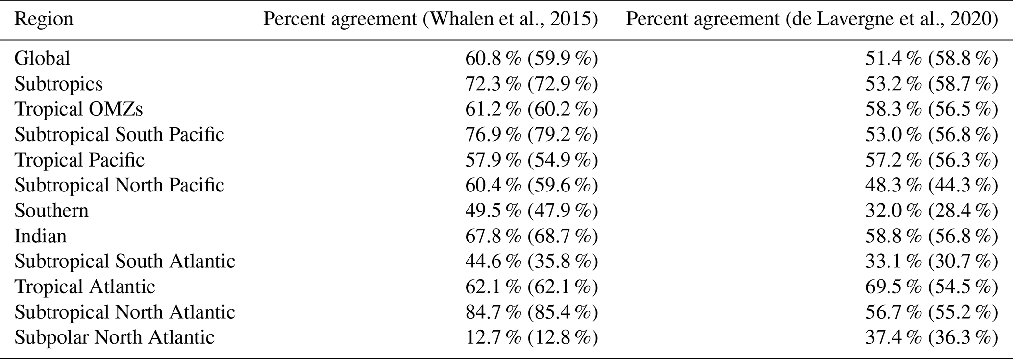
We make use of multiple datasets for κ_ρ derived from observations. Two of these datasets – listed in Table 1 – are derived using a fine-scale parameterization; they contain values equatorwards of 75^∘ S and 75^∘ N and deeper than about 250 m because the theory does not yield accurate results in the presence of strong upper-ocean density variability (e.g., D'Asaro, 2014). κ_ρ values are derived from fine-structure observations of temperature, salinity, and pressure using a strain-based fine-scale parameterization, which has been developed and implemented in different ways (Henyey et al., 1986; Gregg, 1989; Polzin et al., 1995, 2014) but typically assumes a mixing efficiency of 0.2 (St. Laurent and Schmitt, 1999; Gregg et al., 2018). The fine-scale parameterization assumes that (1) the production of turbulent energy at small scales is due to an energy transfer driven by wave–wave interactions down to a wave breaking scale; (2) nonlinearities in the equation of state, double diffusion, downscale energy transports, and mixing associated with boundary layer physics and hydraulic jumps are neglected; and (3) stationary turbulent energy balance exists where production is matched by dissipation and a buoyancy flux in fixed proportions (Polzin et al., 2014). The implementation by Whalen et al. (2015) uses Argo data, assumes a shear-to-strain variance ratio of 3 and a flux Richardson number of Ri_f=0.17, and determines the fraction of turbulent production that goes into the buoyancy flux (and the rest for dissipation). The fine-structure method is not expected to be valid in equatorial regions of the ocean, but nevertheless, the κ_ρ product compares well with microstructure near the Equator (Whalen et al., 2015). We use the 2006–2014 climatology of Whalen et al. (2015) – referred to as κ_ρ,Argo hereafter – which is a gridded product on an approximately $\mathrm{1}{}^{\circ }\times \mathrm{1}{}^{\circ }$ horizontal grid and has three vertical levels: 250–500, 500–1000, and 1000–2000 m depth. Whalen et al. (2015) found that 81 % (96 %) of their κ_ρ,Argo product is within a factor of 2 (3) of the microstructure measurements. We use this as the basis for the factor of 2–3 uncertainty we cite hereafter.

Table 1 The latitude and depth ranges of each observationally derived product from a parameterization used in this study. The longitude range for each dataset spans (180^∘ E, 180^∘ W). Also listed are the time period of the observations each product is based on and the range of values in each product (to the nearest order of magnitude in units of m² s⁻¹).

In addition to the Argo-derived κ_ρ,Argo product, there is ship-based CTD hydrography-derived κ_ρ (Kunze, 2017) – referred to as κ_ρ,CTD hereafter – that uses the same fine-structure parameterization as in the calculation of the κ_ρ,Argo product (see Sect. 2.2). The vertical resolution of the κ_ρ,CTD product is 256 m, and the horizontal resolution is the spacing between each CTD profile. Data are only included in the κ_ρ,CTD product when the square of the buoyancy frequency is greater than 10⁻⁷ rad² s⁻² and greater than the square of the Coriolis frequency, ${\mathit{\kappa }}_{\mathit{\rho },\text{CTD}}<\mathrm{3}\times {\mathrm{10}}^{-\mathrm{3}}$ m² s⁻¹ is positive, and the depth is deeper than 400 m.

One last product we use for observationally derived κ_ρ – referred to as κ_ρ,tides hereafter – is based on theory, a spectral parameterization for abyssal hills, and climatological products (de Lavergne et al., 2020). This scheme accounts for the local breaking of high-mode internal tides and remote dissipation of low-mode internal tides. The four processes contributing to the mixing from this scheme include wave–wave interactions that attenuate low-mode internal tides, shoaling that breaks low-mode internal tides, dissipation of low-mode internal tides at critical slopes, and scattering of low-mode internal tides combined with generation of high-mode internal tides via abyssal hills. Note that these tidally induced mixing process are not equivalent to the suite of internal wave-induced mixing processes that κ_ρ,Argo and κ_ρ,CTD account for. The gridded κ_ρ,tides product is global, nominally $\mathrm{1}/\mathrm{2}{}^{\circ }$ horizontal resolution, and ranges from 10 to 250 m in vertical resolution. A stratification field is provided in this product, which is the one we use for the remainder of this study (Sect. 2.1.3).

2.1.2 Dissolved oxygen

Because we have annual mean κ_ρ products, we use the annual mean dissolved oxygen concentration climatology from the World Ocean Atlas (Garcia et al., 2013) for the remainder of our analysis. Any potential information that oxygen concentrations provide about κ_ρ is likely through oxygen's vertical gradients because water masses – which tend to be relatively homogenous in oxygen concentrations – are eroded via diapycnal mixing along their peripheries. Thus, we show oxygen's vertical gradients, $\partial {\mathrm{O}}_{\mathrm{2}}/\partial z$, here. We compare $\partial {\mathrm{O}}_{\mathrm{2}}/\partial z$ (Fig. 1a, c, and e) with the dissipation rates, $\mathit{ϵ}=N^{\mathrm{2}}{\mathit{\kappa }}_{\mathit{\rho }}/\mathrm{0.2}$, for stratification N² through the Osborn (1980) relationship from the Whalen et al. (2015) product (Fig. 1b, d, and f) at the same depth-averaged bins. $\partial {\mathrm{O}}_{\mathrm{2}}/\partial z$ is generally smaller in magnitude in many high-latitude and tropical regions (Fig. 1a, c, and e), whereas the Argo-derived dissipation rates can be relatively large in these regions, with the exception of locations in the Southern Ocean (Fig. 1b, d, and f). $\partial {\mathrm{O}}_{\mathrm{2}}/\partial z$ is relatively large and positive landward of the Gulf Stream, in the Chukchi Sea and Beaufort Sea, near the Norwegian coast, off the southern coast of India, near the Equator in the Atlantic Ocean and western Pacific Ocean, and in the Southern Hemisphere's subtropical gyres of the Pacific Ocean and Indian Ocean between 250 and 500 m depth (Fig. 1a). The largest positive $\partial {\mathrm{O}}_{\mathrm{2}}/\partial z$ values are between the subpolar regions and the Equator at deeper depths (Fig. 1c and e). The dissipation rates are relatively small in many of these regions (Fig. 1b, d, and f). Exceptions to the inverse relationship between $\partial {\mathrm{O}}_{\mathrm{2}}/\partial z$ and the dissipation rates tend to be in the vicinity of intensified jets, likely because lateral exchanges of oxygen concentrations become more important in these regions. Where data exist for both data products, the spatial correlation between $\partial {\mathrm{O}}_{\mathrm{2}}/\partial z$ and the dissipation rates is about −0.2 and increases in magnitude on coarser grids. This indicates a possibly nonlocal relationship between $\partial {\mathrm{O}}_{\mathrm{2}}/\partial z$ and dissipation rates. The spatial correlation between $\partial {\mathrm{O}}_{\mathrm{2}}/\partial z$ and κ_ρ,Argo is smaller in magnitude – about −0.1 – which motivates further consideration of the information provided by N².

Figure 1 Shown are the vertical gradients of oxygen concentrations (units in $\mathrm{mL}{\mathrm{L}}^{-\mathrm{1}}{\mathrm{m}}^{-\mathrm{1}}$) from the World Ocean Atlas (2013) (panels a, c, and e) and the base-10 logarithms of the dissipation rates (units in W kg⁻¹) from Whalen et al. (2015) (panels b, d, and f). Panels (a) and (b) show an average over 250–500 m depth. Panels (c) and (d) show an average over 500–1000 m depth. Panels (e) and (f) show an average over 1000–2000 m depth. White areas in the ocean indicate insufficient data.

2.1.3 Stratification

We use an observational climatology for N², as provided by the de Lavergne et al. (2020) dataset. N² is generally about 10⁻⁷–10⁻⁵ s⁻², with lower values in high-latitude and deeper regions and higher values in the thermocline and in shallow water areas – which skew its global average (standard deviation) below the mixed layer to about $\mathrm{1.2}\times {\mathrm{10}}^{-\mathrm{4}}$ ($\mathrm{3}\times {\mathrm{10}}^{-\mathrm{3}}$) s⁻². The vertical gradients in N² are typically between $-{\mathrm{10}}^{-\mathrm{5}}$ and 10⁻⁵ ${\mathrm{m}}^{-\mathrm{1}}{\mathrm{s}}^{-\mathrm{2}}$ and have an average value (standard deviation) of about $-{\mathrm{10}}^{-\mathrm{7}}$ ($\mathrm{4}\times {\mathrm{10}}^{-\mathrm{6}}$) ${\mathrm{m}}^{-\mathrm{1}}{\mathrm{s}}^{-\mathrm{2}}$, with its largest magnitudes on continental shelves – high-latitude ones in particular – and in the eastern equatorial Pacific Ocean. The spatial correlation between the annual mean vertical gradients in oxygen (Fig. 1a, c, and e) and the annual mean vertical gradients in N² is about 0.25, which suggests that stratification is one candidate factor in explaining why oxygen concentrations are correlated with κ_ρ and ϵ. However, we do not test this with model experiments that incorporate information about N² – which directly compare N² from our model and observations – because the vertical resolution of our ocean model is so much coarser than that of observations. Instead, we run a set of model experiments that compare oxygen concentrations, κ_ρ, or ϵ. We perform these model experiments to further explore the potential information that oxygen concentrations provide about κ_ρ and indirectly infer – via the Osborn (1980) relation – the possible role of stratification.

2.2 Modeling system

We use the Estimating the Circulation and Climate of the Ocean (ECCO) framework in our analysis. ECCO uses a time-invariant but spatially varying background κ_ρ field – κ_ρ,bg hereafter – calculated with a parameter and state estimation procedure, and κ_ρ associated with temperature and salinity are assumed to be identical. Details about the model simulations we perform are summarized in Table 2.

Table 2 Listed are the ECCO simulations performed and analyzed in the present study as well as the observationally derived data or measured data included in each simulation. Either observationally derived data or measured data are included in the experiments through a misfit calculation (Eq. 1). Here, κ_ρ,obs denotes an observationally derived κ_ρ product derived from a parameterization (κ_ρ,Argo and κ_ρ,CTD or κ_ρ,tides) or inferred from microstructure (κ_ρ,micro), $\mathit{ϵ}={\mathit{\kappa }}_{\mathit{\rho }}{N}^{\mathrm{2}}/\mathrm{0.2}$ indicates an observationally derived dissipation rate (N² is the stratification from the World Ocean Atlas or WOA, 2013), and O₂ is the climatology of measured oxygen concentrations from WOA (2013). The misfits for the experiments with κ_ρ and ϵ are calculated using Eq. (2).

2.2.1 ECCO

The modeling system used here is ECCOv4r3 (Fukumori et al., 2017). The underlying ocean–sea ice model is based on the Massachusetts Institute of Technology general circulation model (MITgcm), which is a global finite-volume model. The ECCOv4r3 global configuration uses curvilinear Cartesian coordinates (Forget et al., 2015a – see their Figs. 1–3) at a nominal 1^∘ (0.4^∘ at the Equator) resolution and rescaled height coordinates (Adcroft and Campin, 2004) with 50 vertical levels and a partial cell representation of bottom topography (Adcroft et al., 1997). The MITgcm uses a dynamic–thermodynamic sea ice component (Menemenlis et al., 2005; Losch et al., 2010; Heimbach et al., 2010) and a nonlinear free surface with freshwater flux boundary conditions (Campin et al., 2004). The wind speed and wind stress are specified as 6-hourly varying input fields over 24 years (1992–2015). Average adjustments to the wind stress, wind speed, specific humidity, shortwave downwelling radiation, and surface air temperature are re-estimated and then applied over 14 d periods. These adjustments are based on estimated prior uncertainties for the chosen atmospheric reanalysis (Chaudhuri et al., 2013), which is ERA-Interim (Dee et al., 2011). The net heat flux is then computed via a bulk formula (Large and Yeager, 2009). The ocean variables, on the other hand, do not get periodically adjusted. A parameterization of the effects of geostrophic eddies (Gent and McWilliams, 1990) is used. Mixing along isopycnals is accounted for according to the framework provided by Redi (1982). Vertical mixing is the sum of diapycnal mixing and the vertical component of the along-isopycnal tensor, with diapycnal mixing determined according to the Gaspar et al. (1990) mixed layer turbulence closure and estimated κ_ρ,bg. Convective adjustment does not act through κ_ρ in the MITgcm. Here, κ_ρ represents a combination of processes, including – but potentially not limited to – internal wave-induced mixing. κ_ρ,bg, the Redi coefficient, and the Gent–McWilliams coefficient are time-independent because of the underdetermined problem of inverting for initial conditions, and model parameters would be even more underdetermined if they were allowed to vary in time – explained below. In order to simulate oxygen concentrations, tracers are carried using the Biogeochemistry with Light, Iron, Nutrients and Gases (BLING) model (Galbraith et al., 2015). BLING is an intermediate-complexity biogeochemistry model that uses eight prognostic tracers and parameterized, implicit representations of iron, macronutrients, and light limitation and photoadaptation. BLING has been shown to compare well with the Geophysical Fluid Dynamics Laboratory's full-complexity biogeochemical model, TOPAZ (Galbraith et al., 2015), and has been adapted for use in the MITgcm with its adjoint (Verdy and Mazloff, 2017).

Initial conditions and model parameters for the runs performed here are from ECCOv4r3. The least-squares problem solved by the ECCO model uses the method of Lagrange multipliers through iterative improvement, which relies upon a quasi-Newton gradient search (Nocedal, 1980; Gilbert and Lemarechal, 1989). Algorithmic (or automatic) differentiation tools (Griewank, 1992; Giering and Kaminski, 1998) have allowed for the practical use of Lagrange multipliers in a time-varying nonlinear inverse problem such as ocean modeling, eliminating the need for discretized adjoint equations to be explicitly hand-coded. Contributions of observations to the model–data misfit function are weighted by the best available estimated data and model representation error variance (Wunsch and Heimbach, 2007). The observational data included in the ECCO state estimation procedure are discussed in Forget et al. (2015a) and Fukumori et al. (2017). These data include satellite-derived ocean bottom pressure anomalies, sea ice concentrations, sea surface temperatures, sea surface salinities, sea surface height anomalies, and mean dynamic topography, as well as profiler- and mooring-derived temperatures and salinities (Fukumori et al., 2017). No ocean subgrid-scale transport parameter, mixing parameter, or biogeochemical tracer data are included in the model's misfits during the parameter and state estimation procedure. The control variables that are inverted for iteratively by ECCO are listed in Table 3, which include the ocean subgrid-scale transport and mixing parameters – e.g., κ_ρ,bg. The error covariances for each of the ocean subgrid-scale transport and mixing parameters are specified by imposing a smoothness operator (Weaver and Courtier, 2001) at the scale of three grid points – which corresponds to a decorrelation length scale diameter of ∼100 km – which allows the dynamical model to regionally adjust from the information provided by observations (Forget et al., 2015b). A total of 59 iterations of the parameter and state estimation procedure – referred to as the “optimization” run hereafter – were performed to arrive at the ECCOv4r3 solution we start from for our experiments. The resulting κ_ρ,bg field in the ECCOv4r3 solution – plus the Gaspar et al. (1990) contribution – will be referred to as κ_ρ,ECCO hereafter and is shown in Fig. 2 depth-averaged below the model's average mixed layer depth. Note that the initial guess for κ_ρ,bg in ECCO is 10⁻⁵ m² s⁻¹, and in the absence of observation-driven adjustments, κ_ρ,bg in ECCO remains at or is close to its initial value in the ECCOv4r3 solution, at least in its depth average. Also note that in regions away from ocean boundary layers, κ_ρ,ECCO is approximately κ_ρ,bg in ECCO. κ_ρ,ECCO is elevated in regions that undergo deep convection, near the margins of continental shelves and intensified jets, and in the Indonesian Throughflow. We will later compare κ_ρ,ECCO with κ_ρ from the first iteration of the same optimization run with ECCO, which will be referred to as ${\mathit{\kappa }}_{\mathit{\rho },\text{ECCO},\mathrm{0}}$ hereafter. If ${\mathit{\kappa }}_{\mathit{\rho },\text{ECCO},\mathrm{0}}$ is in closer agreement with κ_ρ from observational products than κ_ρ,ECCO, then errors in κ_ρ,ECCO are likely being compensated for by errors in other control variables beyond the first iteration of the model's optimization run.

(Redi, 1982)(Gent and McWilliams, 1990)

Table 3 The control variables that ECCO inverts for and optimizes. Some of these control variables are initial conditions only (indicated in the “initial condition” column). Other control variables are time-varying (indicated in the “time-varying” column). The rest are not initial conditions but also are time-independent. Also noted is whether the control variable's field is two-dimensional or three-dimensional – there are no control variables that vary in both time and over all locations and depths of the ocean.

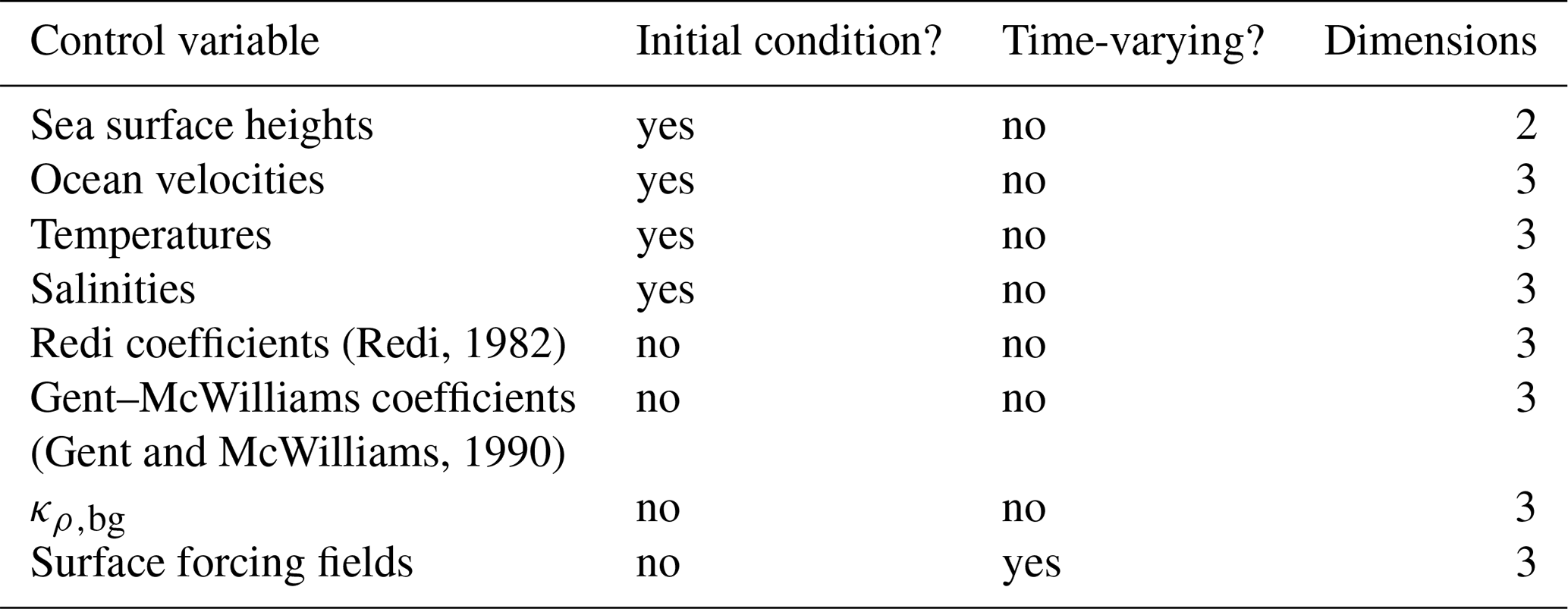
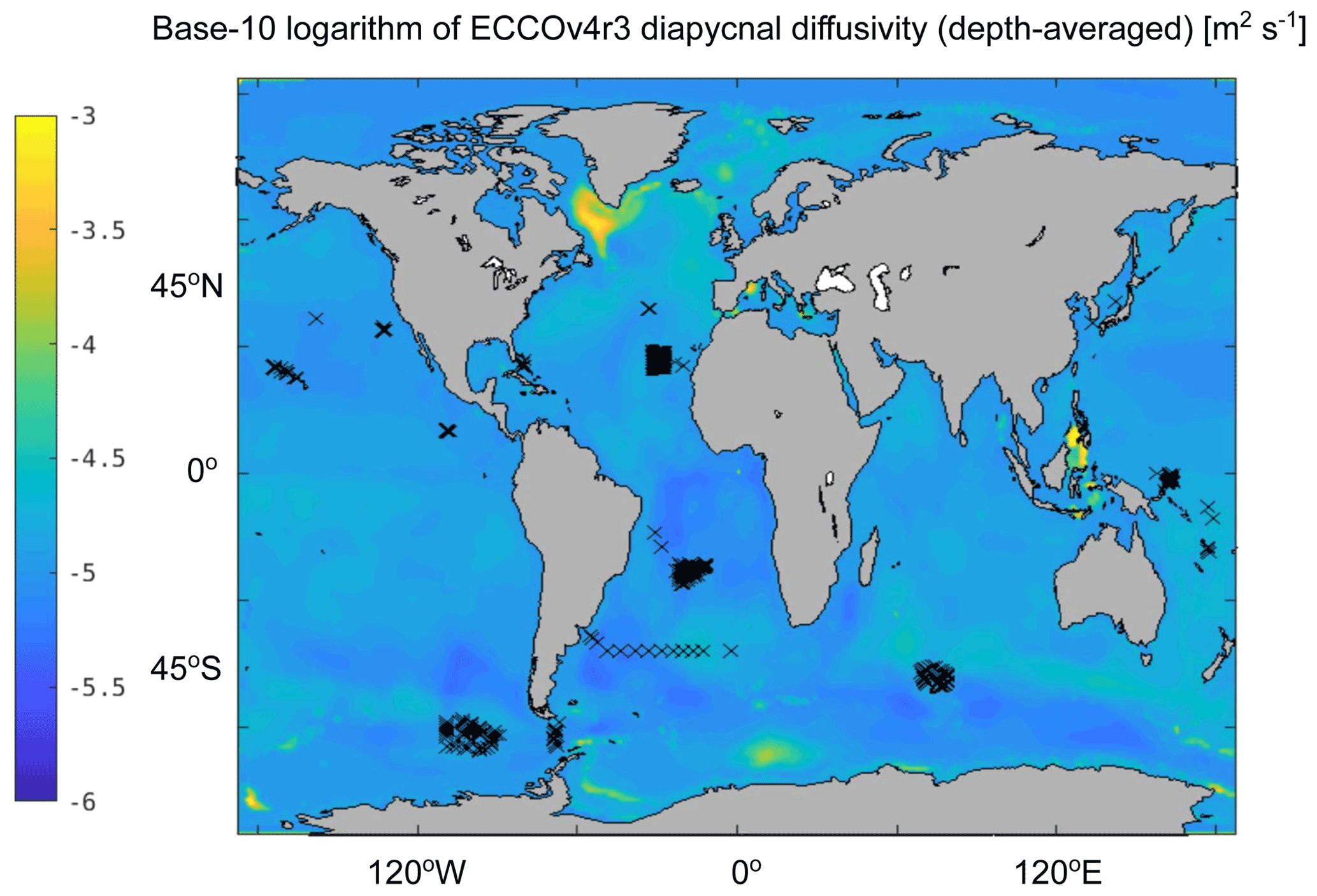
Figure 2 Shown is the base-10 logarithm of κ_ρ,ECCO (units in m² s⁻¹), depth-averaged over all depths below the average mixed layer depth to exclude very large values within the mixed layer. Black X marks indicate locations where there are microstructure measurements used in this study.

We run ECCO in two configurations: (1) a “re-run,” wherein all control variables are set to their estimated values from ECCOv4r3 in forward mode – sometimes referred to as an ocean-only free run – and (2) an “adjoint sensitivity” run of the parameter and state estimate in forward plus adjoint modes, wherein data are included in the model's misfits but not technically “assimilated” because the model input parameters do not change as the model runs. An adjoint sensitivity is essentially the sensitivity of one variable to another, computed by making use of the model's adjoint. Formally, an adjoint sensitivity is $\partial J/\partial X$, where the cost function J is a sum of weighted misfits to observations and a control variable X is a variable that the model estimates by making use of its adjoint and observations – see Sect. 2.2.2. The adjoint sensitivities provide information about which directions the model's input parameters should change X in order to minimize J. Masuda and Osafune (2021) showed some examples of adjoint sensitivities of several model parameters in their ocean state estimate to a vertical mixing parameter (slightly different from κ_ρ). We also compute adjoint sensitivities in the present study, but using ECCO with respect to X=κ_ρ.

The following is a summary of the ECCO experiments we run (Table 2).

• E-CTRL is a forward ECCOv4 simulation that uses the parameters from ECCOv4r3; this simulation can be referred to as a re-run.

• E_O is an adjoint sensitivity (with respect to X=κ_ρ) experiment in which only oxygen concentrations from the World Ocean Atlas (2013) climatology are included in the misfit function J.

• E_κ is an adjoint sensitivity (with respect to X=κ_ρ) experiment in which only the base-10 logarithm of the κ_ρ,micro dataset, κ_ρ,Argo and κ_ρ,CTD products, or κ_ρ,tides product is included in the misfit function J.

• E_ϵ is an adjoint sensitivity (with respect to X=ϵ) experiment in which only the base-10 logarithm of the ${\mathit{ϵ}}_{\text{Argo}}={\mathit{\kappa }}_{\mathit{\rho },\text{Argo}}{N}^{\mathrm{2}}/\mathrm{0.2}$ and ${\mathit{ϵ}}_{\text{CTD}}={\mathit{\kappa }}_{\mathit{\rho },\text{CTD}}{N}^{\mathrm{2}}/\mathrm{0.2}$ products or the ${\mathit{ϵ}}_{\text{tides}}={\mathit{\kappa }}_{\mathit{\rho },\text{tides}}{N}^{\mathrm{2}}/\mathrm{0.2}$ product is included in the misfit function J.

The difference between experiment E_κ and E_ϵ is that the latter uses observationally derived dissipation rates, $\mathit{ϵ}=N^{\mathrm{2}}{\mathit{\kappa }}_{\mathit{\rho }}/\mathrm{0.2}$ instead of κ_ρ, in the misfit function via Eq. (2). We do not perform experiment E_ϵ with microstructure data included in the model's misfit function because of the sparsity of those data. We analyze the adjoint sensitivities with dissipation rates in the misfit function (E_ϵ in Table 2) in order to assess whether the stratification – a multiplying factor between κ_ρ and the dissipation rates according to Osborn (1980) – provides information about κ_ρ. Due to the relatively coarse vertical resolution of ECCO compared with observations, we do not directly compare N² from ECCO with N² from observations in another adjoint sensitivity experiment.

We take the ECCOv4r3 solution as the reference state for each of our simulations. We perform an adjoint calculation in each experiment, except for E-CTRL. The adjoint sensitivities are accumulated and averaged over the full integration period. Only 1 year was run for each of the adjoint simulations, but our results are not qualitatively sensitive to the run length – which is at least partially because we use time-invariant climatologies. The time dependence of the κ_ρ sensitivities from E_κ is weak due to the lack of time dependence of the observations included in the misfits – κ_ρ and oxygen concentrations; initial condition sensitivities are stronger. Thus, our simulations will suffice to demonstrate whether the inclusion of a biogeochemical tracer in the model's misfits can reduce the bias in κ_ρ.

We begin E_O from a previously derived product that has been spun up from an initial climatology (Fig. 3a) derived from World Ocean Atlas (2013). Thus, disagreements with the World Ocean Atlas (2013) are due to model drift. The depth-averaged differences between the uninterpolated World Ocean Atlas (2013) product and the initial conditions for oxygen concentrations in our ECCO run using BLING are shown in Fig. 3b. The differences are largest in the Arctic Ocean, northeastern Pacific Ocean, and near the coasts, particularly on the eastern side of the American continent, the southwestern side of the African continent, around the Kuroshio and Sea of Japan region, along almost every coastline of Oceania, and in the Mediterranean Sea (Fig. 3b). Pointwise differences between the initial conditions for oxygen concentrations in ECCO and the World Ocean Atlas (2013) product are shown in Fig. 3c, which suggests that there is strong agreement between the two fields. Where there are disagreements, the initial conditions for oxygen concentrations in ECCO are more often too small (particularly in the Atlantic Ocean, as shown in Fig. 3b) than too large. These differences are likely due to the deficiencies in model resolution, the sparse observations in regions such as the Arctic Ocean, the locations of sea ice (Bigdeli et al., 2017), and the parameterization of the tracer air–sea fluxes (e.g., Atamanchuk et al., 2020). We need to consider the spatial patterns shown in Fig. 3b when interpreting the signs of the adjoint sensitivities.

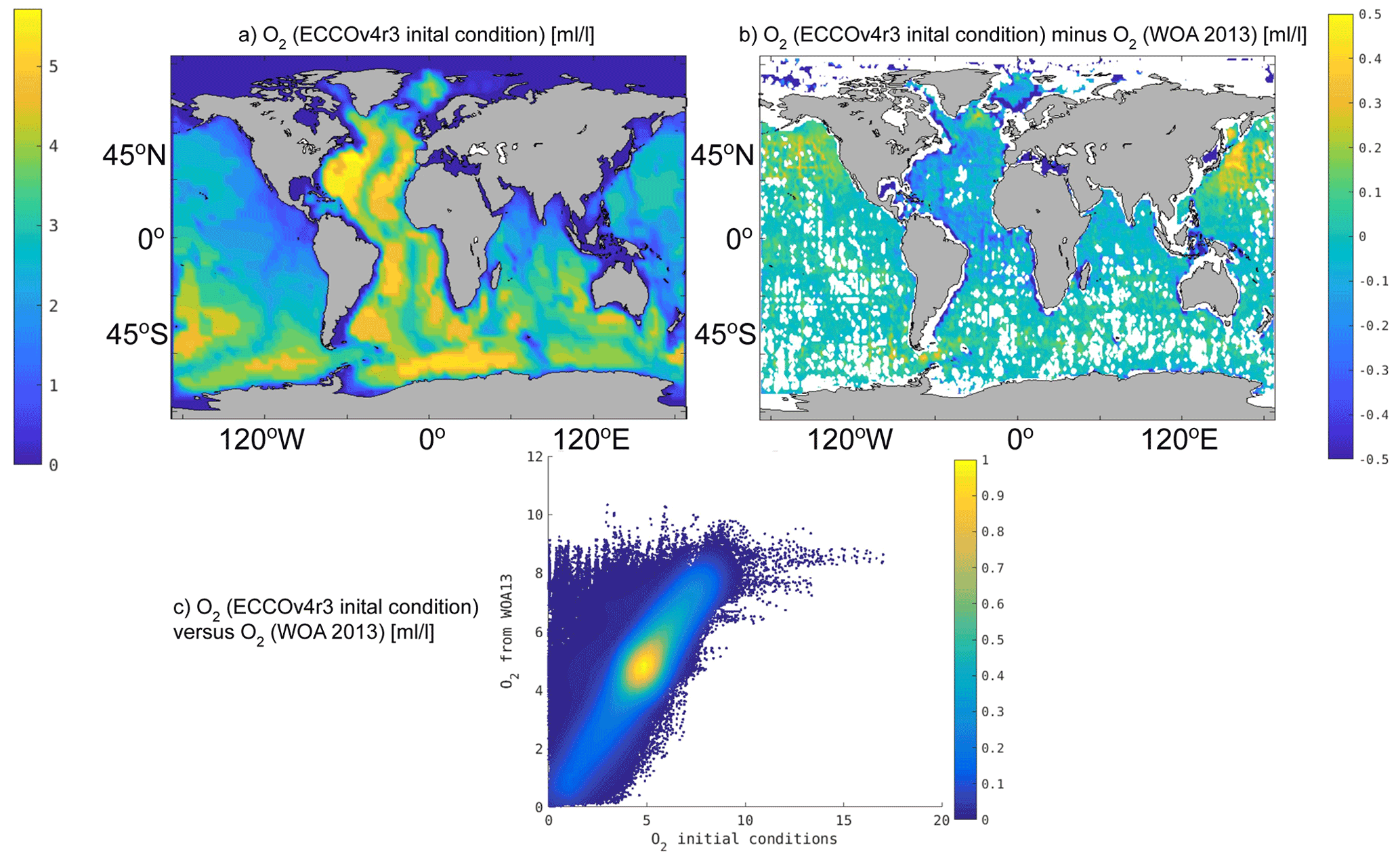
Figure 3 Shown are (a) the depth-averaged oxygen concentrations' initial conditions in ECCO (units in mL L⁻¹), (b) the depth-averaged oxygen concentrations' initial conditions in ECCO minus the depth-averaged observational climatologies from the World Ocean Atlas (2013) (units in mL L⁻¹) at locations where observations were sampled, and (c) the pointwise comparisons between the oxygen concentrations' initial conditions and the observational climatologies from the World Ocean Atlas (2013) (units in mL L⁻¹), which are used for the ECCO adjoint sensitivity experiments in the model's cost function. White areas in panel (b) in the ocean indicate insufficient data to calculate a depth average.

2.2.2 ECCO adjoint sensitivity analyses

Short of including a particular dataset (e.g., dissolved oxygen concentrations) in the misfits of a new optimization run of ECCO, we assess whether the inclusion of a particular dataset in the model's misfits could lead to a more accurate estimate of a control variable that can be observed (e.g., κ_ρ). In order to understand whether κ_ρ could be estimated more accurately through the inclusion of oxygen concentrations in the model's misfit, we need to further explain the details of our adjoint sensitivity experiments with ECCO. We define the objective (or cost) function here to more formally explain what the adjoint sensitivity is. ECCO calculates the cost function to be minimized, J (Stammer et al., 2002) – focusing here only on the observational misfit terms while omitting regularization terms for the control variables – as

$$\begin{array}{}\text{(1)}& J=\sum _{t=\mathrm{1}}^{t_{\mathrm{f}}}{\left[\mathit{y}\left(t\right)-\mathbf{S}\stackrel{\mathrm{̃}}{\mathit{x}}\left(t\right)\right]}^T\mathbf{W}\left(t\right)\left[\mathit{y}\left(t\right)-\mathbf{S}\stackrel{\mathrm{̃}}{\mathit{x}}\left(t\right)\right]\end{array}$$

where t_f is the final time step, $\stackrel{\mathrm{̃}}{\mathit{x}}$ is the model-based estimate of the state vector x, S is the observation matrix that relates the model state vector to observed variables y (such that $\mathbf{S}\stackrel{\mathrm{̃}}{\mathit{x}}$ is the model-based estimate of the observables y), and W is the weight (inverse square of approximate uncertainties accounting for measurement and representation errors) of the observations. In each of our adjoint sensitivity experiments, the data vector y only contains the dataset specific to the experiment (see Table 2), so we emphasize here that J is different for each of our experiments. The uncertainties in κ_ρ,ECCO in E_κ are set to be 3 times the values of the observationally derived κ_ρ because of the level of agreement between κ_ρ,Argo and κ_ρ,micro (Whalen et al., 2015). The uncertainties in oxygen concentrations in E_O are set to be 2 % of the values of the measured dissolved oxygen concentrations.

The adjoint sensitivities computed in this study are the derivatives of J in Eq. (1) with respect to κ_ρ. We consider evaluating directions in the control space in which to improve κ_ρ through improvement of κ_ρ,bg, given the control vector from the ECCOv4r3 solution. While the adjoint sensitivities of J to the control space in experiment E_O must be computed online, those in E_κ can either be computed online or offline using an analytical equation (see below). The adjoint sensitivity run with κ_ρ included in the misfit calculation of experiment E_κ can be calculated offline using output from the E-CTRL run instead of being calculated online as follows:

$$\begin{array}{}\text{(2)}& {\displaystyle \frac{\partial J}{\partial X}}=-\mathrm{2}{\displaystyle \frac{\left(X_{\text{obs}}-X_{\text{model}}\right)}{{\mathit{\sigma }}_X^{\mathrm{2}}}}.\end{array}$$

Here, X=κ_ρ is the control variable, X_obs is the observationally derived value of X described in the previous section, X_model is the value that ECCO estimates for X, and σ_X is taken to be $\mathrm{3}{X}_{\text{obs}}/\mathrm{1.96}$ (or the base-10 logarithm of this in the case of κ_ρ) due to the factor of 3 uncertainty corresponding to an approximate 95 % confidence interval in Whalen et al. (2015). For X_model, we use the offline values calculated from the E-CTRL run following Eq. (2). While this assumes a diagonal W and minimal impact of the smoothing operator applied over a decorrelation length scale diameter of ∼100 km, the offline Eq. (2) and online sensitivities have been verified to be in agreement.

Because the observations of κ_ρ here are not direct measurements, we first need to show that observationally derived κ_ρ has a smaller bias with respect to independent observations than the model's estimate of κ_ρ. We devote the first portion of our study to determining whether $|{\mathit{\kappa }}_{\mathit{\rho },\text{Argo}}-{\mathit{\kappa }}_{\mathit{\rho },\text{micro}}|<|{\mathit{\kappa }}_{\mathit{\rho },\text{ECCO}}-{\mathit{\kappa }}_{\mathit{\rho },\text{micro}}|$ (and, by extension, κ_ρ,CTD in place of κ_ρ,Argo) is true. We do this because κ_ρ,micro is limited in its spatial coverage compared to κ_ρ,Argo, κ_ρ,CTD, and κ_ρ,tides. Also, κ_ρ,Argo and κ_ρ,CTD are still limited in spatial coverage relative to dissolved oxygen concentrations. While κ_ρ,tides has global spatial coverage, its measurement and structural uncertainties are not well-known compared to dissolved oxygen concentrations. The data product with higher accuracy (dissolved oxygen concentrations) will have larger weights (W in Eq. 1) and will thus exert more influence in constraining κ_ρ,ECCO – bringing it closer to microstructure values. So if we can show that the adjustments to κ_ρ in ECCO are similar, whether we provide information from observationally derived κ_ρ or a measured tracer with relatively small uncertainties (dissolved oxygen concentrations), then we would include the tracer in the misfits.

One problem with doing a direct comparison of the adjustments is that the uncertainties in observationally derived κ_ρ products are large, so we first quantify the extent to which the adjoint sensitivities from two runs (here, E_κ and E_O) have the same sign at each location and depth. Specifically, we inspect whether $\partial J/\partial {\mathit{\kappa }}_{\mathit{\rho }}$ has the same sign in E_κ and E_O, where $|{\mathit{\kappa }}_{\mathit{\rho },\text{Argo}}-{\mathit{\kappa }}_{\mathit{\rho },\text{ECCO}}|$ is significantly different from zero (i.e., κ_ρ,Argo is more than a factor of 3 greater or less than a factor of 3 smaller than κ_ρ,ECCO). We are interested in regions where κ_ρ is significantly erroneous and where the errors in oxygen are due to errors in the physics (e.g., κ_ρ), not initial conditions: hence, these choices. We perform these comparisons in regions where the difference between the observationally derived κ_ρ products and κ_ρ,ECCO exceeds 3 times the observational products' magnitudes (i.e., statistically distinguishable from zero). Because model errors unrelated to κ_ρ can confound the correlations between the adjoint sensitivities from E_κ and E_O, we additionally look at regions where the difference between oxygen concentrations from the model and the World Ocean Atlas (2013) is relatively small to determine whether oxygen concentrations guide the state estimate's control space to improve the magnitude of κ_ρ. In this subset of regions, we calculate the correlations between the adjoint sensitivities from E_κ and E_O – despite the difficulty with determining their significance.

To investigate whether the results are sensitive to our assumptions about the signal-to-noise ratio of our data – through W in Eq. (1) – we additionally perform Monte Carlo simulations for the adjoint sensitivities from E_κ – using three different datasets for κ_ρ: κ_ρ,micro, κ_ρ,Argo together with κ_ρ,CTD, and κ_ρ,tides. In the Monte Carlo simulations, at each location and depth, we randomly sample κ_ρ values within its uncertainty – σ_κ – simultaneously with randomly sampled values of σ_κ between a factor of 2–3 of κ_ρ. This accounts for the uncertainties in the κ_ρ products in both the numerator – corresponding to uncertainties in the observationally derived estimates – and denominator of Eq. (2) – corresponding to the weights. With each of the 10 000 samples of κ_ρ and σ_κ, we recompute the adjoint sensitivity for E_κ and then its correlation with that for E_O. With these Monte Carlo simulations, we report the maximum possible correlation between each experiment's adjoint sensitivities.

3 Results

We first show that the disagreements between κ_ρ from ECCO and κ_ρ from various observations are larger than the observations' approximate 95 % confidence intervals. Then we analyze results from pairs of adjoint sensitivity runs: one with misfits to observed κ_ρ derived from the fine-scale parameterization and the other with misfits to observed O₂. We use these results to investigate the potential to use O₂ as a constraint for improving κ_ρ,ECCO in a future optimization. We then compare the results of the adjoint sensitivity runs using misfits in κ_ρ with ones using misfits in ϵ to infer a potential role of stratification in any information that O₂ provides about κ_ρ. In the Appendix, we show there is general agreement between κ_ρ from observations and a free-running Earth system model that calculates a physically motivated parameterization for κ_ρ, but there is poor agreement between κ_ρ from observations and a sequential ocean data assimilation system based on the same Earth system model (Fig. A1a).

3.1 Model-inverted vs. microstructure-inferred κ_ρ comparisons

We compare the average κ_ρ,micro profile that is comprised of 24 campaigns' worth of data (Waterhouse et al., 2014) (see their Fig. 6; black curves in Figs. 4a and 5) with average κ_ρ,ECCO profiles from two different iterations and the κ_ρ,Argo product (Whalen et al., 2015). The locations of the microstructure measurements are shown in Fig. 2 (black X marks). We also compare the average κ_ρ,tides profile (de Lavergne et al., 2020) (see their Fig. 2e; black curve in Fig. 4b) with the average κ_ρ,ECCO profile from the final iteration.

Figure 4 (a) κ_ρ profiles averaged over all microstructure observation locations (shown in Fig. 2) from the first iteration of the optimization (E-CTRL₀ – grey curve) and from the (final) 59th iteration of the optimization (E-CTRL – blue curve). Also shown is the average of κ_ρ profiles from the full-depth microstructure observations (black curve) presented in Waterhouse et al. (2014) (see their Fig. 6; also see Fig. 5 of the present study) with 1 spatial standard deviation flanking the average (dashed black curves) and an approximate factor of 3 uncertainty flanking the average (dotted black curves), as well as the average of κ_ρ (magenta X marks) at each of the depth bins in the Whalen et al. (2015) product. At each location, the simulated profiles are extracted and the base-10 logarithms of the geometric averages of the observed and ECCO-estimated κ_ρ (units in m² s⁻¹) are shown. (b) κ_ρ profiles averaged over the entire ocean from the 59th iteration of the optimization (E-CTRL – blue curve) and from the de Lavergne et al. (2020) tidal mixing product (black curve).

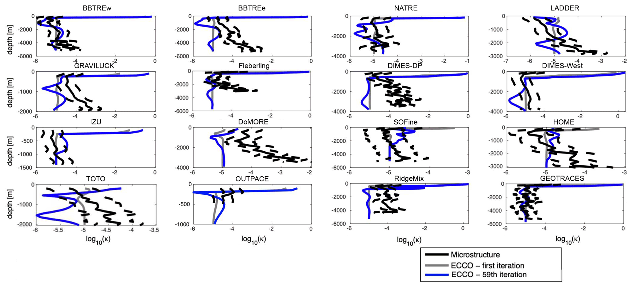
Figure 5 In each panel, κ_ρ profiles are shown averaged over 16 example microstructure observation campaigns (see Fig. 2): from the first iteration of the optimization (E-CTRL₀ – grey curve), from the (final) 59th iteration of the optimization (E-CTRL – blue curve), and from the full-depth microstructure observations (black curve) presented in Waterhouse et al. (2014) (see their Fig. 6). Approximate factor of 3 uncertainties flanking the κ_ρ profiles from microstructure are shown with dashed black curves.

The average ${\mathit{\kappa }}_{\mathit{\rho },\text{ECCO},\mathrm{0}}$ profile – i.e., the first adjusted initial guess of κ_ρ,ECCO – is typically smaller than the microstructure profile, particularly at 1000 m where the difference is approximately an order of magnitude (Fig. 4a). At iteration 59 (which is the ECCOv4r3 solution), the difference between κ_ρ,ECCO and κ_ρ,micro decreases. However, agreement between the average profiles of κ_ρ,ECCO and κ_ρ,micro is still worse than the agreement between κ_ρ,Argo and κ_ρ,micro. The agreement between κ_ρ,Argo and κ_ρ,micro at each of the three depth bins is well within a factor of 3 (dotted black curves in Fig. 4a) and the spatial standard deviation of κ_ρ,micro (dashed black curves in Fig. 4a). The agreement between the average profiles of κ_ρ,ECCO and κ_ρ,tides is poor, with κ_ρ,ECCO typically too small, notably so at deeper depths (Fig. 4b). κ_ρ,ECCO includes internal-wave-induced mixing as well as potentially numerical diffusion. However, numerical diffusion cannot explain the errors in κ_ρ,ECCO, where κ_ρ is too small in the model relative to the observationally derived products because numerical diffusion would increase κ_ρ,ECCO. In these regions, one likely explanation is that errors in other model parameters (e.g., the Redi coefficients) compensate for the errors in κ_ρ,bg.

We also compare κ_ρ,ECCO and ${\mathit{\kappa }}_{\mathit{\rho },\text{ECCO},\mathrm{0}}$ profiles with κ_ρ,micro from 16 example campaigns in Fig. 5. In some regions, the κ_ρ,ECCO and ${\mathit{\kappa }}_{\mathit{\rho },\text{ECCO},\mathrm{0}}$ profiles are constant (10⁻⁵ m² s⁻¹, the default background value) because ECCO does not sufficiently resolve the bathymetry, so we exclude those from Fig. 5. We also exclude some others, for example, in the subpolar North Atlantic Ocean because temporal variations in κ_ρ can be large there (Fig. A1b). The κ_ρ,ECCO profiles (blue curves in Fig. 5) and ${\mathit{\kappa }}_{\mathit{\rho },\text{ECCO},\mathrm{0}}$ profiles (grey curves in Fig. 5) are often within the approximate (factor of 3) uncertainties in the κ_ρ,micro profiles (dashed black curves in Fig. 5), but not always. Without taking an average over all of the campaigns, there can be large regional disagreements between the model and observations. Also, the κ_ρ,ECCO profiles are not always closer to the κ_ρ,micro profiles than the ${\mathit{\kappa }}_{\mathit{\rho },\text{ECCO},\mathrm{0}}$ profiles. This suggests that performing more iterations of the optimization of ECCO is not necessarily going to lead to more accurate representation of κ_ρ with the current data constraints.

3.2 Model-inverted vs. fine-scale parameterization-derived κ_ρ comparisons

We next show κ_ρ,Argo and κ_ρ,tides as well as how they contrast with κ_ρ,ECCO because this highlights the spatial patterns of the adjoint sensitivities in E_κ (see later). The ratio between the κ_ρ,Argo product (Fig. 6a, c, and e) and κ_ρ,ECCO varies throughout the globe (Fig. 6b, d, and f). Red (blue) areas in Fig. 6b, d, and f indicate locations where Argo-derived κ_ρ,Argo is smaller (larger) than κ_ρ,ECCO. The percent of volume for which κ_ρ,ECCO is at least an order of magnitude different from κ_ρ,Argo is 43.8 %. The values of κ_ρ,ECCO are smaller than those in the Argo- and hydrography-derived observational product in the Kuroshio Extension (500–1000 m depth), subpolar North Atlantic Ocean (500–1000 m depth), Southern Ocean, equatorial regions in the Atlantic Ocean, and shallow (250–500 m depth) Indian Ocean and eastern Pacific Ocean (Fig. 6b, d, and f). In contrast, κ_ρ,ECCO tends to be too large relative to the κ_ρ,tides product (Fig. 7a, c, and e) in the Atlantic Ocean below 500 m depth as well as in many near-equatorial and subpolar regions, and κ_ρ,ECCO tends to be too small everywhere else (Fig. 7b, d, and f). Regardless of the observational product, the κ_ρ,ECCO field is comparatively large in many of the model's near-equatorial regions, where the intermittency of strong mixing events is likely not captured – even in a time-mean sense – because the ECCO framework uses a smoother. However, the fidelity of each observational product is unknown near the Equator. The fact that κ_ρ,ECCO and each observational product disagree within the deep mixed layers at high latitudes is not consequential for tracer transport. The errors in κ_ρ,bg could be partially compensating for errors in the vertical component of the along-isopycnal diffusivity tensor, erroneous air–sea fluxes due to inconsistencies between the sea surface and atmospheric forcing fields, and/or the presence of numerical diffusion.

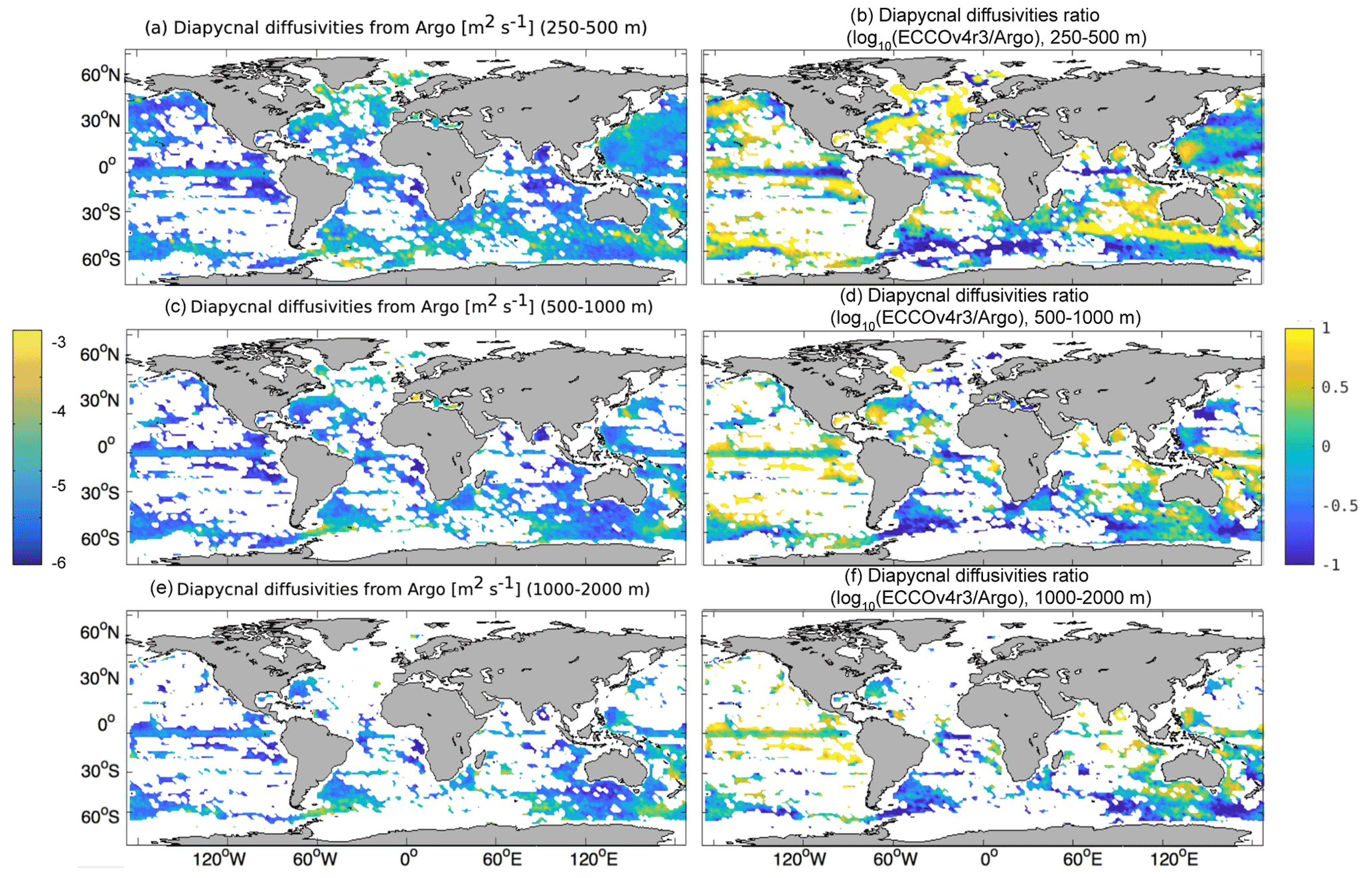
Figure 6 Shown are (a, c, and e) the base-10 logarithms of κ_ρ,Argo (units in m² s⁻¹) and (b, d, and f) the base-10 logarithms of the ratios of the time-averaged κ_ρ,ECCO to κ_ρ,Argo. Panels (a) and (b) show an average over 250–500 m depth. Panels (c) and (d) show an average over 500–1000 m depth. Panels (e) and (f) show an average over 1000–2000 m depth. White areas in the ocean indicate insufficient Argo data to derive κ_ρ,Argo.

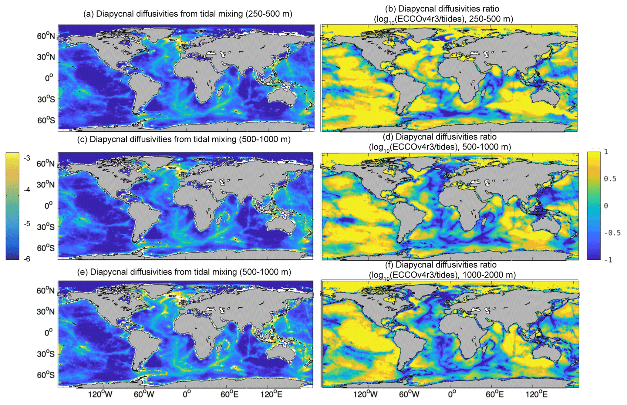
Figure 7 Shown are (a, c, and e) the base-10 logarithms of κ_ρ,tides (units in m² s⁻¹) and (b, d, and f) the base-10 logarithms of the ratios of the time-averaged κ_ρ,ECCO to κ_ρ,tides. Panels (a) and (b) show an average over 250–500 m depth. Panels (c) and (d) show an average over 500–1000 m depth. Panels (e) and (f) show an average over 1000–2000 m depth.

Incomplete historical observations – of temperature, salinity, and pressure – are currently insufficient to accurately estimate κ_ρ,bg – approximately κ_ρ,ECCO away from the boundary layers, where we compare with observational products. Even the abundance of Argo data in the upper 2000 m has not been enough to calculate a realistic κ_ρ,ECCO in the upper 2000 m. The sparsity of the observations below 2000 m depth, in high-latitude regions, and in some near-coastal areas – where internal wave-induced mixing can be important – is relevant because complete observational coverage of the ocean's temperature, salinity, and pressure could, in principle, better constrain κ_ρ,bg using inverse modeling (Groeskamp et al., 2017). However, the lack of time dependence of κ_ρ,bg, the presence of numerical mixing, and joint estimation of many underdetermined parameters in ECCO could also lead to erroneous κ_ρ,ECCO. These are some reasons why values of κ_ρ,ECCO do not agree well with κ_ρ from observations – κ_ρ,micro, κ_ρ,Argo, κ_ρ,CTD, or κ_ρ,tides.

3.3 Adjoint sensitivities in ECCO

Because the data that are currently included in ECCO's misfits are insufficient for κ_ρ,ECCO to match κ_ρ,micro, κ_ρ,Argo, κ_ρ,CTD, or κ_ρ,tides, including additional variables controlled by mixing in the model's misfits may assist in further improving the modeled mixing parameters. Oxygen is a candidate since its distribution is, in part, determined by the local κ_ρ. To test this, we run multiple adjoint sensitivity experiments in which either observationally derived κ_ρ or oxygen is included in the misfit calculation to guide constraints on κ_ρ. We expect the signs of sensitivities to agree most in regions away from where air–sea fluxes and transport of oxygen – e.g., by intensified jets – are large. One of these regions is the subtropical North Atlantic Ocean, away from the Gulf Stream Extension. Further, we expect to find more agreement between the signs of sensitivities in tropical OMZs and other (sub)tropical regions because of the known importance of diapycnal mixing in these regions.

We show the adjoint sensitivity calculations using Eq. (2) for κ_ρ misfits (experiment E_κ in Table 2) in Fig. 8 using κ_ρ,Argo and κ_ρ,CTD; these are later compared with the sensitivities for oxygen concentration misfits in experiment E_O. A positive adjoint sensitivity implies that the misfit can be reduced by decreasing κ_ρ,ECCO. The signs of $\partial J/\partial {\mathit{\kappa }}_{\mathit{\rho }}$ using κ_ρ,Argo and κ_ρ,CTD (Fig. 8a) are consistent with the signs of local disagreement with microstructure (Figs. 4a and 5) and Argo-derived observations (Fig. 6b, d, and f) by construction. Because κ_ρ,ECCO tends to be very large inside mixed layers, $\partial J/\partial {\mathit{\kappa }}_{\mathit{\rho }}$ tends to be positive and larger at many locations in the subpolar latitudes where there are deep mixed layers in the model but possibly not in the real ocean; conversely, $\partial J/\partial {\mathit{\kappa }}_{\mathit{\rho }}$ can be negative where the mixed layer depth is too shallow in ECCO, but this is not the only reason for $\partial J/\partial {\mathit{\kappa }}_{\mathit{\rho }}<\mathrm{0}$. The large positive values of $\partial J/\partial {\mathit{\kappa }}_{\mathit{\rho }}$ within the mixed layer and some other regions overwhelm the zonal averages in favor of positive values (Fig. 8c). κ_ρ,ECCO needs to be decreased in many regions at depths shallower than 500 m to agree better with κ_ρ,Argo and κ_ρ,CTD (yellow regions in Fig. 6b, d, and f), but microstructure measurements (X marks in Fig. 2) were often taken in locations where κ_ρ,ECCO should be increased (blue regions in Fig. 6b, d, and f) or stay the same. Microstructure measurements tend to be regions where there are prominent topographic features and where the centers of subtropical gyres are found, which – judging from the predominant signs of disagreement in Figs. 4a and 5 versus Fig. 6b, d, and f – are not representative of the ocean where Argo measurements were taken.

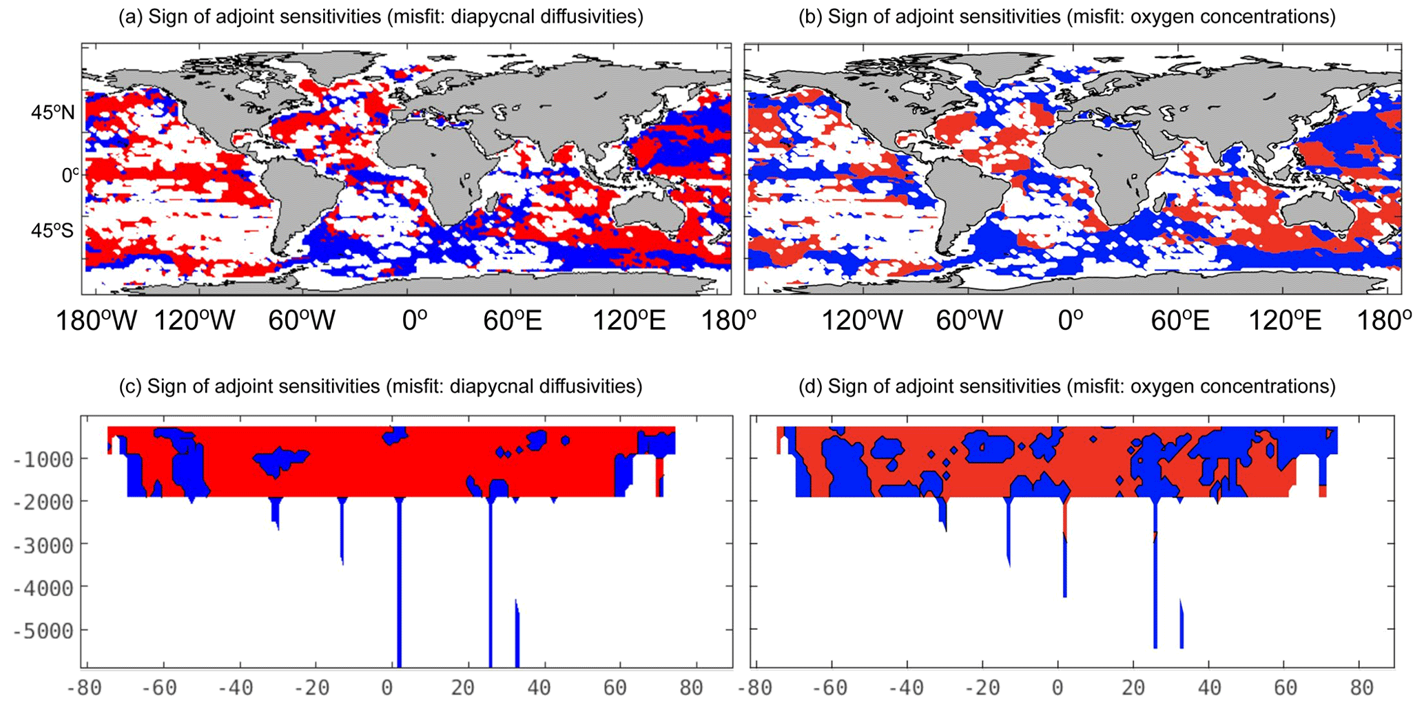
Figure 8 Adjoint sensitivity sign comparisons: results from E_κ – using the Whalen et al. (2015) and Kunze (2017) products – (panels a and c) and E_O (panels b and d) are shown for the adjoint sensitivities (units in s m⁻²) with respect to κ_ρ averaged over 250–2000 m depth (panels a and b) and zonally averaged (panels c and d). The red regions indicate that the adjoint sensitivities are positive ($\partial J/\partial {\mathit{\kappa }}_{\mathit{\rho }}>\mathrm{0}$), and blue regions indicate negative adjoint sensitivities. κ_ρ,Argo and κ_ρ,CTD are the only quantities used in the misfit calculation of an adjoint run shown in panels (a) and (c). The climatological oxygen concentrations from the World Ocean Atlas (2013) are the only observations used in the misfit calculation of a separate adjoint run shown in panels (b) and (d). The adjoint sensitivities in panels (a) and (c) are computed offline (i.e., not using ECCO, but by plugging in the value the model reads in for the base-10 logarithm of κ_ρ and comparing that with the above observationally derived base-10 logarithm of the κ_ρ products using the fine-scale parameterization via Eq. 2). The adjoint sensitivities in panels (b) and (d) are computed online (i.e., using ECCO, which uses the base-10 logarithm of κ_ρ as a control variable). The white regions are locations with bathymetry or insufficient observations. The adjoint sensitivities are calculated over just 1 year (1992).

We next compare $\partial J/\partial {\mathit{\kappa }}_{\mathit{\rho }}$ from E_κ using κ_ρ,Argo and κ_ρ,CTD with $\partial J/\partial {\mathit{\kappa }}_{\mathit{\rho }}$ from E_O. In E_O, $\partial J/\partial {\mathit{\kappa }}_{\mathit{\rho }}$ is generally negative in subtropical regions (Fig. 8b and d). Overall, the locations of the positive and negative signs of $\partial J/\partial {\mathit{\kappa }}_{\mathit{\rho }}$ are not the same everywhere between the E_κ and E_O experiments, but they agree in many regions (Fig. 8a and c and Fig. 8b and d) using κ_ρ,Argo and κ_ρ,CTD, which account for nearly two-thirds (three-fourths) of the ocean's volume where they can be compared (in the subtropics, between 20 and 50^∘ N and S; Fig. 9 and Table 4). The ocean basin with the highest percent volume of agreement in adjoint sensitivity signs between E_κ and E_O is the subtropical North Atlantic Ocean, with nearly 85 % volume agreement. The subtropical South Atlantic Ocean is the only subtropical basin with less than half of its volume in agreement in adjoint sensitivity sign. In general, the tropical regions (between 20^∘ S and 20^∘ N) have adjoint sensitivity signs in lesser agreement than the subtropical regions, and the subpolar regions (poleward of 50^∘ N and S) are the regions with the lowest percent volume agreements in adjoint sensitivity signs.

Figure 9 Adjoint sensitivity sign comparisons: shown are the percents of volume over the water column for each horizontal location (panel a) and percent of volume over all longitudes for each depth and latitude (panel b) where the sign of $\partial J/\partial {\mathit{\kappa }}_{\mathit{\rho }}$ agrees between E_κ – using the Whalen et al. (2015) and Kunze (2017) products – and E_O. The white areas are locations where the disagreements between κ_ρ,ECCO and κ_ρ,Argo supplemented with κ_ρ,CTD are within 3 times the value of the observationally derived κ_ρ, so these were excluded.

(Whalen et al., 2015)(de Lavergne et al., 2020)

Table 4 Listed are the percent volumes for which the signs of the adjoint sensitivities agree between E_κ – for both the Whalen et al. (2015) and de Lavergne et al. (2020) products – and E_O for different regions of the ocean. The boundaries of subtropical–equatorial regions are set to be at 20^∘ N and S. The boundaries of subtropical–subpolar and subtropical–Southern Ocean regions are set to be 50^∘ N and S. The tropical oxygen minimum zones (OMZs) are where oxygen concentrations are less than 2 mL L⁻¹ between 20^∘ S and 20^∘ N. The percentages are only calculated when sufficient observations are available to derive κ_ρ and when the difference between the model-calculated and observationally derived κ_ρ is greater than the uncertainty (i.e., 3 times the observationally derived κ_ρ). In parentheses are the same, except for the dissipation rates, ${\mathit{ϵ}}_{\mathit{\rho }}=N^{\mathrm{2}}{\mathit{\kappa }}_{\mathit{\rho }}/\mathrm{0.2}$, where N² is the stratification and 0.2 is an empirical coefficient (see, e.g., Gregg et al., 2018).

We also show the adjoint sensitivity calculations using Eq. (2) for κ_ρ misfits (experiment E_κ in Table 2) in Fig. 10 using κ_ρ,tides and compare $\partial J/\partial {\mathit{\kappa }}_{\mathit{\rho }}$ from E_κ using κ_ρ,tides with $\partial J/\partial {\mathit{\kappa }}_{\mathit{\rho }}$ from E_O. The signs of $\partial J/\partial {\mathit{\kappa }}_{\mathit{\rho }}$ using κ_ρ,tides (Fig. 10a) are consistent with the signs of local disagreement with the de Lavergne et al. (2020) product (Figs. 4b and 7b, d, and f) by construction. The positive values of $\partial J/\partial {\mathit{\kappa }}_{\mathit{\rho }}$ outside the Atlantic Ocean and in the vicinity of intensified jets overwhelm the zonal averages in favor of positive values at most depths (Fig. 10c). κ_ρ,ECCO needs to be decreased in many regions at depths shallower than about 2500 m to agree better with κ_ρ,tides (Fig. 4b; yellow regions in Fig. 7b, d, and f). The regions where κ_ρ,ECCO needs to be increased become dominant closer to the seafloor, particularly in the Atlantic Ocean. The signs of $\partial J/\partial {\mathit{\kappa }}_{\mathit{\rho }}$ from E_κ agree with $\partial J/\partial {\mathit{\kappa }}_{\mathit{\rho }}$ from E_O in fewer regions (Fig. 10a and c and Fig. 10b and d) using κ_ρ,tides instead of κ_ρ,Argo and κ_ρ,CTD. The regions with agreement in signs of sensitivities using κ_ρ,tides account for just over half of the ocean's volume where they can be compared globally (Fig. 11 and Table 4); this is also true for the subtropics. The equatorial regions have the highest percent volume of agreement in signs of sensitivities using κ_ρ,tides over all depths, but the North Atlantic Ocean also has fairly high agreement (Fig. 11a). There is high agreement in the regions of the Arctic Ocean that are north of the Greenland and Barents seas too. Compared with shallower depths, regions below 3000 m depth tend to be derived from Antarctic Bottom Water (Marshall and Speer, 2012 – see their Fig. 1) and therefore have different oxygen concentration characteristics such as weaker vertical gradients. They also have differences between κ_ρ,ECCO and observationally derived κ_ρ that are more commonly statistically indistinguishable and have less overwhelmingly positive adjoint sensitivities from E_κ using κ_ρ,tides (Fig. 10c). As a result, all of the depths with the highest levels of agreement in signs of sensitivities using κ_ρ,tides are between the mixed layer depth and 3000 m depth (Fig. 11b). Most differences in the spatial distribution of agreements between the signs of sensitivities across different observationally derived products (Figs. 9 and 11) are at least partially due to their spatial coverage – Argo versus global – and the <100 % overlap in processes accounted for by the various κ_ρ products. Thus, the level of agreement in signs of sensitivities from E_κ and E_O is high over many regions and is qualitatively consistent in its spatial distribution across the different observationally derived products for κ_ρ.

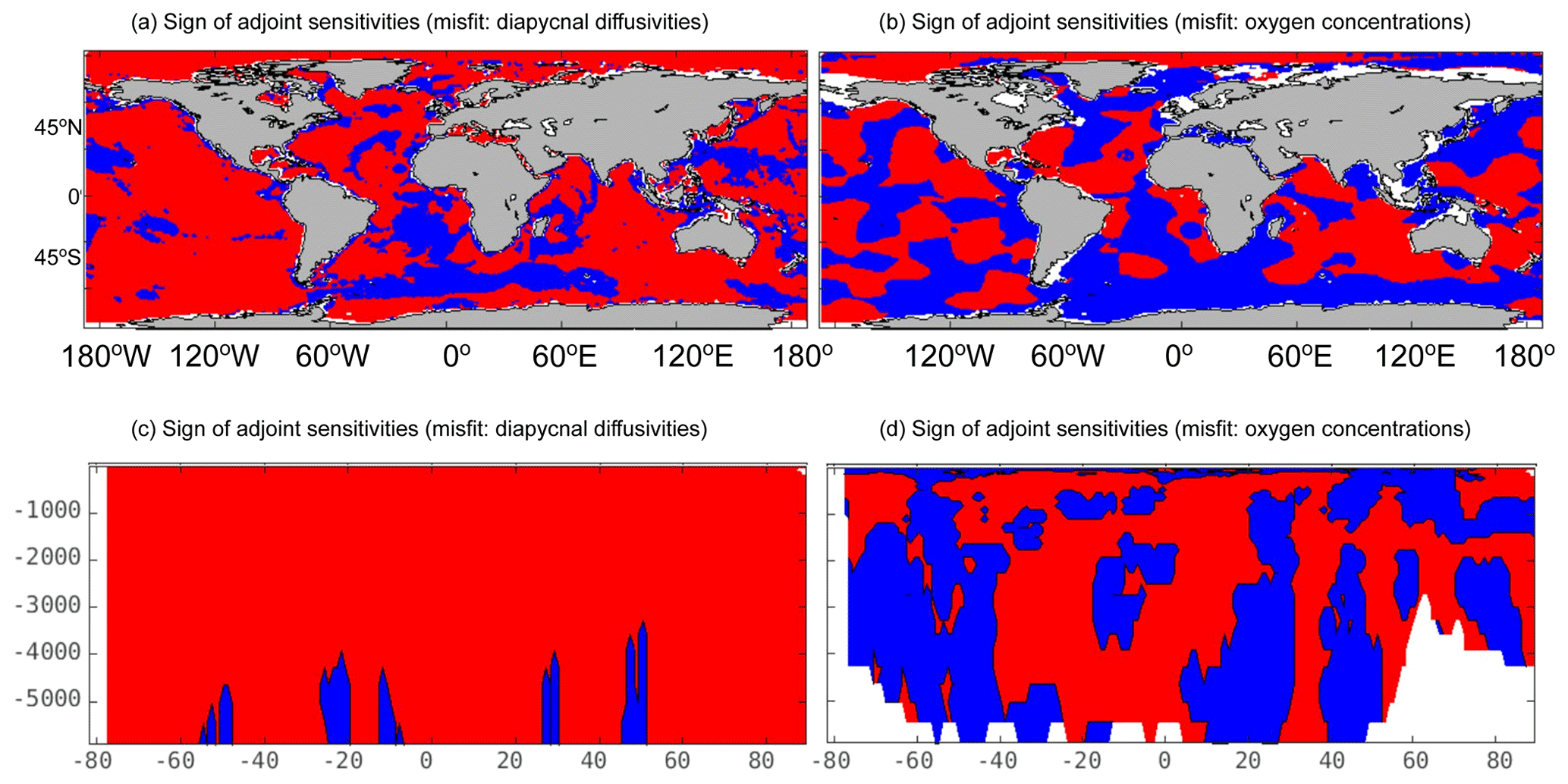
Figure 10 Adjoint sensitivity sign comparisons: same as Fig. 8, but with the de Lavergne et al. (2020) product, κ_ρ,tides.

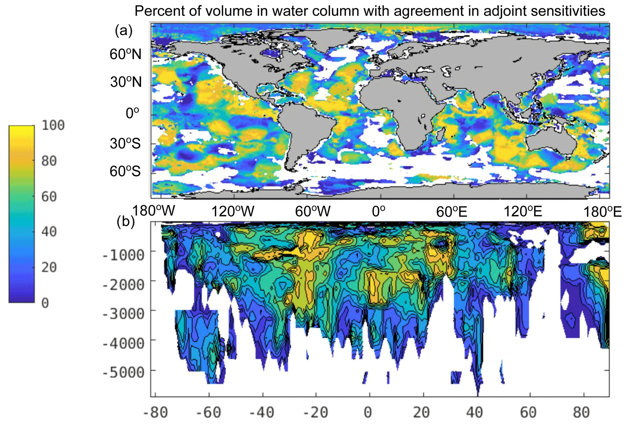
Figure 11 Adjoint sensitivity sign comparisons: same as Fig. 10, except using the de Lavergne et al. (2020) product, κ_ρ,tides.

We need to address whether any of the agreement in signs of sensitivities is random – as their correlation is due to the large uncertainties in observationally derived κ_ρ – or underpinned by physical reasons. We first focus on the locations with statistically indistinguishable errors in κ_ρ,ECCO. These regions and those where there can be significant differences between oxygen concentrations in ECCO and the World Ocean Atlas (2013) product correspond to the white regions in Fig. 9 that are red or blue in Fig. 8 – likewise for Fig. 11 versus Fig. 10. The vast majority of the locations where disagreements occur in sensitivity signs are in places with statistically indistinguishable differences between κ_ρ,ECCO and observationally derived κ_ρ. The regions with statistically indistinguishable differences in κ_ρ account for 56.2 % (24.1 %) of the volume of the ocean where the adjoint sensitivities from E_O and E_κ can be compared using κ_ρ,Argo and κ_ρ,CTD (κ_ρ,tides). Thus, we exclude a large portion of the ocean from the remainder of our analysis because we cannot determine whether agreements in signs of sensitivities are by random chance in these regions.

We next inspect the sensitivity sign patterns in regions with statistically significant κ_ρ misfits. The regions where the signs of $\partial J/\partial {\mathit{\kappa }}_{\mathit{\rho }}$ agree from the two experiments and have large differences between κ_ρ,ECCO and the combined κ_ρ,Argo and κ_ρ,CTD product tend to have relatively small oxygen concentration misfits (Fig. 3b). This is also true when using the κ_ρ,tides product. For example, when only regions with less than 1 standard deviation above the average oxygen concentration misfits are selected, the signs of the adjoint sensitivities agree between E_O and E_κ over 60.8 % (50.5 %) of the volume with sufficient data using κ_ρ,Argo and κ_ρ,CTD (κ_ρ,tides). However, the larger the oxygen concentration misfits, the more often the signs of the sensitivities agree. When only regions with more than 3 standard deviations above the average oxygen concentration misfits are selected, the signs of the sensitivities always agree. Thus, the regions with the largest disagreements in oxygen concentrations can always decrease their oxygen misfits by changing κ_ρ,ECCO with a sign consistent with decreasing its disagreement with observationally derived κ_ρ, wherever differences in κ_ρ are detectable.

Where there are statistically significant differences in κ_ρ, we still need to determine whether there is a physical basis for the agreements in signs of sensitivities. We next show results that are consistent with our hypothesis that tropical OMZs and other (sub)tropical regions are where oxygen concentrations can inform κ_ρ in the model such that there is better agreement with observationally derived κ_ρ products. The regions with the highest percent volume agreement in sensitivity signs, regardless of which observationally derived κ_ρ product is used, include tropical OMZs and other (sub)tropical regions below several hundred meters of depth (Figs. 9b and 11b). Differences between the signs of the sensitivities tend to be more common in locations where κ_ρ is not expected to dominate the variability in oxygen. These regions include, for example, the open subpolar North Atlantic Ocean (e.g., the Labrador Sea in Figs. 9a and 11a), where Atamanchuk et al. (2020) present observational evidence that air–sea fluxes mediated by bubble injection – not represented by ECCO – dominate the variability in oxygen down to 1000 m depth. While there can be a high percent volume agreement in sensitivity signs in the equatorial Pacific Ocean and Atlantic Ocean, these are also regions where Palter and Trossman (2018) and Brandt et al. (2021) point out that ocean circulation changes significantly influence long-term changes in oxygen. This suggests that changes in both ocean circulation and κ_ρ could be important in explaining oxygen concentration variations in the tropics. When the tropical and subpolar regions (outside the 20–50^∘ N and S bands) are excluded, the percent volume of the ocean where the signs of the adjoint sensitivities agree between E_κ and E_O increases, regardless of which observationally derived κ_ρ product we use. Given that there are known physical processes not dominated by κ_ρ causing variations in oxygen concentrations in regions outside tropical OMZs and other (sub)tropical regions, our interpretation of the patterns shown in Figs. 8–11 is that κ_ρ controls much of the variability in oxygen concentrations in large portions of tropical OMZs and other (sub)tropical regions. This is one indication that dissolved oxygen concentrations could provide information about κ_ρ, at least for some regions of the ocean.

We further address whether the potential information dissolved oxygen concentrations provide about κ_ρ is due to the information oxygen contains about stratification. To determine whether oxygen provides information about stratification – and through stratification, about κ_ρ – we use the adjoint sensitivity results obtained from experiment E_ϵ with observationally derived dissipation rates, $\mathit{ϵ}=N^{\mathrm{2}}{\mathit{\kappa }}_{\mathit{\rho }}/\mathrm{0.2}$ (e.g., Fig. 1b, d, and f) instead of κ_ρ (e.g., Fig. 6b, d, and f), in the misfit function via Eq. (2) and multiply the adjoint sensitivity of E_O by $\mathrm{0.2}/N^{\mathrm{2}}$ so that their sensitivities are each taken with respect to ϵ (parentheses in Table 4). We find approximately equal agreement between the signs of the adjoint sensitivities from E_O (scaled by $\mathrm{0.2}/N^{\mathrm{2}}$) and E_ϵ as we do between those from E_O and E_κ in every region, regardless of which observationally derived product we use. Because ϵ is related to κ_ρ through the stratification, we suggest that the information oxygen concentrations provide about κ_ρ is likely independent of the stratification field.

Lastly, given that the general agreement in signs of sensitivities between E_κ and E_O is likely underpinned by physical reasons unrelated to stratification, we pursue whether there is a statistically significant relationship between the adjoint sensitivities from E_κ and E_O. We again focus on the regions where the difference between κ_ρ,ECCO and observational κ_ρ products (from tides, Argo/CTD, and microstructure) is statistically significant (greater than a factor of 3), but also filter out the adjoint sensitivities when the differences between oxygen concentrations from ECCO and those from the World Ocean Atlas (2013) are statistically significant. The simple correlations between the adjoint sensitivities from E_κ and E_O in the remaining regions tend to be small but positive (Fig. 12). In addition to taking simple correlations, we performed Monte Carlo simulations to get a maximum possible correlation between each experiment's adjoint sensitivities. The maximum correlations from the Monte Carlo simulations are larger than the simple correlations. This is particularly the case when the adjoint sensitivities are both negative (Fig. 12a, c, and e) but is also true when the adjoint sensitivities are both positive (Fig. 12b, d, and f). If we only consider comparing locations where we have both observationally derived κ_ρ data and oxygen data, our results are qualitatively the same and the correlations increase to as much as 0.47 in the case of the κ_ρ,tides product using a Monte Carlo approach. If we further only consider regions where the vertical gradients in stratification are less than their global mean and where the vertical gradients in oxygen concentrations are greater than their global mean, the correlations are approximately the same, indicating that the information oxygen provides about κ_ρ is not conditional on the stratification. This suggests that κ_ρ,ECCO may be constrained by the information provided by oxygen concentrations. That is, oxygen concentrations inform adjoint sensitivities that typically direct κ_ρ,ECCO to improve relative to observationally derived κ_ρ. However, inclusion of accurately known oxygen concentrations in the model's misfits is not a perfect substitute for the inclusion of accurately known κ_ρ itself in the model's misfits.

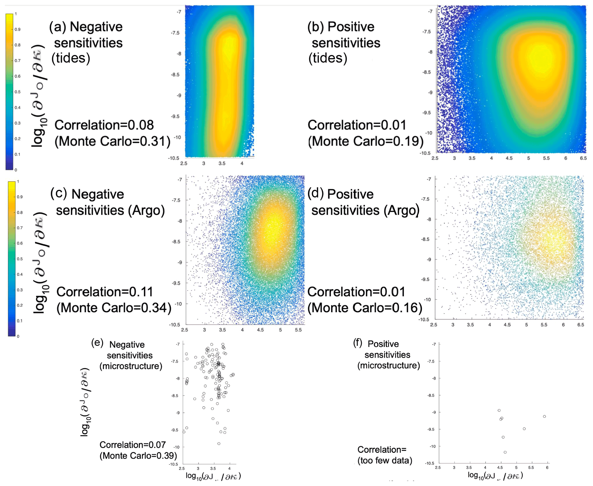
Figure 12 Shown are scatterplots between the adjoint sensitivities from E_O and E_κ where they are both negative (panels a, c, and e) and where they are both positive (panels b, d, and f). E_κ has its adjoint sensitivities calculated with the tidal mixing product κ_ρ,tides (panels a and b), Argo-derived κ_ρ (κ_ρ,Argo and κ_ρ,CTD; panels c and d), or microstructure-inferred κ_ρ (panels e and f). Only the adjoint sensitivities for which the differences between κ_ρ,ECCO and observational κ_ρ products are statistically significant (greater than a factor of 3) and when the differences between oxygen concentrations from ECCO and those from the World Ocean Atlas (2013) are statistically insignificant (within 2 % of the latter) are included. The correlations for all of the data points shown in each panel are listed. Also listed below each panel are the maximum possible correlations from a Monte Carlo-based approach in which 10 000 random samples of κ_ρ within the uncertainties of the observational κ_ρ products are used to recompute the adjoint sensitivities for E_κ.

4 Discussion and concluding remarks

4.1 Discussion

This study evaluated the potential to improve the diapycnal diffusivities (κ_ρ) in the ECCOv4 ocean parameter and state estimation framework. We assessed the fidelity of κ_ρ,ECCO by first comparing the average vertical profiles of κ_ρ,ECCO with those inferred from microstructure. The comparison was not favorable. In regions where we compare with observational products, κ_ρ,ECCO is approximately κ_ρ,bg in ECCO, which is inverted for through constraints of vertical profiles of temperature and salinity – e.g., from Argo profiles. Model choices – e.g., the initial guess of background ${\mathit{\kappa }}_{\mathit{\rho }}={\mathrm{10}}^{-\mathrm{5}}$ m² s⁻¹ everywhere – can lead to errors in κ_ρ,ECCO even in the presence of globally complete hydrographic observations (see Sect. 4.2), but we investigated whether κ_ρ,ECCO can benefit from new information.

We then investigated which additional observations can be used as new constraints to improve the fidelity of the inverted κ_ρ,ECCO. The products we used were observationally derived κ_ρ based on Argo and ship-based CTD hydrographic data, observationally derived κ_ρ based on climatological and seafloor data, and climatological oxygen concentrations. To justify the use of the observationally derived κ_ρ products, we also evaluated them by comparing them with the microstructure-inferred product. κ_ρ,Argo and κ_ρ,CTD have better agreement with the microstructure-inferred data than κ_ρ,ECCO does.

We inspected the misfit of the model parameter κ_ρ,ECCO with respect to κ_ρ,Argo and κ_ρ,CTD as well as to κ_ρ,tides and motivated the use of dissolved oxygen concentration data as a potential constraint in ECCO. One drawback of the observationally derived data products for κ_ρ is that they have large uncertainties – here approximated by a factor of 3. Observed oxygen concentrations, on the other hand, have relatively small uncertainties. More importantly, we showed that vertical oxygen gradients have geographical patterns similar to energy dissipation rates. We therefore performed an additional adjoint sensitivity experiment with oxygen concentration data as the only data in the misfit function. Adjoint sensitivity results were compared between the experiment with measured oxygen in the misfit function and observationally derived κ_ρ in the misfit function. Regions where the sensitivities agree in signs between the two experiments are locations where adjustments in κ_ρ, as informed by these data, can potentially help improve κ_ρ,ECCO. These regions include well over half of the volume of comparable seawater in the (sub)tropical regions – including tropical OMZs. These spatial patterns are consistent with where we expected κ_ρ to explain much of the variability in oxygen concentrations. Correlations between adjoint sensitivities from each experiment are positive when differences between the oxygen concentrations in the model and observations are relatively small. These findings suggest that dissolved oxygen concentrations could be used to more accurately estimate κ_ρ through κ_ρ,bg in a newly optimized ECCO solution. However, given the magnitudes of the correlations between the adjoint sensitivities, inclusion of observationally derived κ_ρ in the model's misfits could (additionally) be necessary, especially if their uncertainties are reduced.

4.2 Caveats and future directions

Many factors – including a significant absence of independent observations for assessment, a combination of measurement and structural errors, numerical diffusion in our simulations, and unconstrained parameters in the biogeochemical modules – have stymied progress in state estimation of ocean subgrid-scale transport and mixing parameters. First, the observational measurement errors used here are only approximate. We assumed uncertainties equal to a factor of 3 of the observationally derived κ_ρ and 2 % of the oxygen concentrations. These do not account for interpolation and/or averaging errors that entered the data prior to our calculations but are conservative estimates nonetheless. The observational uncertainties affect the weights given in the misfits that enter the adjoint sensitivity calculations, and our Monte Carlo simulations of the correlations between the adjoint sensitivities account for the possibility that these weights are misspecified. Second, only one ocean subgrid-scale transport or mixing parameter – namely, κ_ρ – has been compared with independent observational data microstructure. This is the primary reason why we focused on κ_ρ in our study. Third, the ECCO-estimated κ_ρ,bg accounts for other model errors – e.g., structural ones suggested by Polzin et al. (2014) – which explains some of the model biases relative to microstructure observations. For instance, the ECCO-estimated κ_ρ,bg should be time-dependent as well as spatially varying, but it is only spatially varying. In the presence of other estimated model parameters and initial conditions, some parameters could be compensating for errors in κ_ρ,bg. The ECCO-estimated κ_ρ,bg can also be sensitive to the a priori estimate of κ_ρ,bg, and we showed how one particular initial guess – 10⁻⁵ m² s⁻¹ everywhere – can evolve from the first optimization iteration to the final one. Additionally, there is numerical diffusion in the model, which could confound some physical inferences about the model – e.g., regarding how sensitive the model's state is to κ_ρ,bg relative to along-isopycnal diffusion. Numerical errors could remain and result in the primary source of error in the ocean state estimate even if additional constraints are placed on κ_ρ,bg in ECCO. Retaining a parameter which absorbs structural model errors that are not expressed in the model's functional form may be necessary to improve the ECCO state estimate itself, but minimizing numerical errors would be beneficial to improve the ECCO-estimated κ_ρ,bg. Lastly, there are several unconstrained parameters in biogeochemical modules used to calculate biogeochemical tracers (Verdy and Mazloff, 2017), so some of the disagreements in signs of the adjoint sensitivities found here could be associated with other inaccurate parameters.

These challenges can continue to be overcome by allowing models and observations to inform each other. First, the observationally derived κ_ρ from the fine-scale parameterization could be further scrutinized using ship-based CTD data taken concurrently with microstructure velocity shear data. A preliminary analysis suggests that the percent difference between the full depth-averaged CTD-derived κ_ρ from the fine-scale parameterization and the microstructure-inferred κ_ρ at the same locations is 1.68 %, which is indistinguishable from zero, but the quality of the CTD data taken concomitantly with microstructure has not been fully assessed. Second, we can potentially overcome several computational challenges to improve κ_ρ,bg. One example of this is to account for the time dependence of κ_ρ,bg in a future ocean state estimate, but the underdetermined nature of the parameter estimation procedure makes this difficult. These efforts would also benefit from minimizing spurious mixing due to numerical diffusion (e.g., Holmes et al., 2021) through choosing a different advection scheme, but this would add computational expense. If the goal is to improve the other control variables and the state estimate itself – instead of estimating κ_ρ,bg with ECCO – then we could potentially reduce the influence of numerical diffusion and other confounding factors in the estimation of κ_ρ,bg by no longer treating κ_ρ,bg as a control variable. Using an observationally derived κ_ρ, such as the de Lavergne et al. (2020) product, would make the estimation of other control variables less underdetermined, but this would not resolve the problem with a lack of time dependence of κ_ρ,bg nor would it assuage potential problems with model drift. One potential solution to this is to use the de Lavergne et al. (2020) product for κ_ρ,bg and use the Prandtl number as a control variable to help determine the vertical viscosities. This would help with the problem of neither the estimation of underdetermined parameters nor time dependence of κ_ρ,bg, but it could help with numerical issues. Third, we could potentially circumvent the issue of unconstrained parameters in the biogeochemical modules. One potential way to do this is by including preformed oxygen – i.e., oxygen without any biological influence, making it a passive tracer – in the model's misfits instead of oxygen concentrations. Observationally derived transit-time distributions with a maximum entropy-based method from previous studies (e.g., Khatiwala et al., 2009; Zanna et al., 2019) or from a tracer-informed ocean state estimate (DeVries and Holzer, 2019) can help derive preformed oxygen from oxygen concentration observations. Fourth, we could optimize the information from existing oxygen observations with the purpose of constraining κ_ρ. One way to do this is to run observing system experiments. A complementary approach that uses the effective proxy potential framework of Loose and Heimbach (2021) could also help indicate whether measurements of oxygen concentrations in particular locations are redundant or more informative of κ_ρ than in other locations. We did not pursue this in the present study because our adjoint runs use a global misfit. If we perform an ensemble of adjoint sensitivity runs with a single observation in each run, then we could calculate the effective proxy potential at each of these observation locations. Lastly, the (imperfectly known) initial conditions of biogeochemical tracers will also need to be included in the input control vector during optimization of the ocean state estimate. If biogeochemical tracers are included in the misfit calculation in an optimization run, their impact on variables such as κ_ρ would depend upon how they are weighted relative to the physical variables – e.g., temperature, salinity, and pressure. A more complete representation and understanding of κ_ρ are possible through these analyses and methods.

Appendix A: Model with a sequential data assimilation framework

A1 GEOS-5 and the GMAO S2S Ocean Analysis

To demonstrate a problem with κ_ρ in a sequential data assimilation framework, we present example output from a reanalysis product and output from an identical ocean model hindcast without any data assimilation. GEOS-5 includes a global, finite-volume atmospheric general circulation model that is used for numerical weather prediction, seasonal to decadal forecasts, and as the background field for atmospheric reanalyses (Molod et al., 2015). The ocean is represented by the GFDL Modular Ocean Model (Griffies et al., 2015) version 5 (MOM5) and the Los Alamos Community Ice CodE sea ice model (Hunke et al., 2013) version 4.1 (CICE4.1). We use a configuration of the GEOS-5 modeling system with a 1^∘ (0.5^∘ at the Equator) resolution on a tripolar (Murray, 1996) staggered Arakawa B-grid (Mesinger and Arakawa, 1976) and 50 geopotential levels for MOM5, 2^∘ resolution and 24 pressure levels for the atmospheric model, and 1^∘ resolution and three layers for CICE4.1. Historical aerosols (sulfate, dust, and sea salt) and biomass burning emissions (black and organic carbon) updated from the Goddard Chemistry Aerosol Radiation and Transport (GOCART) model (Chin et al., 2002) are used over the time period 1992 through 2016. Initial conditions are based on a long spin-up that used MOM4 coupled to one version of the GEOS-5 atmosphere model (Molod et al., 2012) and hundreds of additional years of spin-up that used MOM4 coupled to a slightly different version of the GEOS-5 atmosphere model. The differences between the two versions of the GEOS-5 atmospheric model used in the two phases of spin-up include developments in cloud microphysics and atmospheric chemistry.

κ_ρ, Redi coefficients, and Gent–McWilliams coefficients are determined in MOM5 as follows. κ_ρ in MOM5 – κ_ρ,GEOS5 hereafter – is represented by the K-Profile Parameterization (KPP; Large et al., 1994) and a parameterization for mixing due to internal tides (Simmons et al., 2004). Shear-driven mixing, gravitational instabilities that can cause vertical convection, and double-diffusive processes, which can cause the temperature diffusivity to be different from the salinity diffusivity, are accounted for in the interior (Large et al., 1994). The resulting κ_ρ,GEOS5 field spatiotemporally varies. However, this combination of parameterizations does not make use of an explicit energy budget that accounts for conversion between kinetic and potential energy when determining κ_ρ,GEOS5. The Redi coefficients (Redi, 1982) and Gent–McWilliams coefficients of the (Gent and McWilliams, 1990) parameterization for mesoscale eddies are, by default, prescribed to be 600 m² s⁻¹ everywhere, except for some variation in western boundary current regions for the Gent–McWilliams coefficients. The Redi coefficients and Gent–McWilliams coefficients are thus constant in time and in most locations. A mixed layer instability scheme for the submesoscale transport by Fox-Kemper et al. (2011) is used.

We use a reanalysis product, which uses the same underlying modeling system as the GEOS-5 coupled Earth system model, called the Global Modeling and Assimilation Office sub-seasonal to seasonal (GMAO S2S) Ocean Analysis. The output of the GMAO S2S Ocean Analysis highlights how κ_ρ can behave due to the disruption of dynamical balance that can be the result of the use of a sequential data assimilation system (Stammer et al., 2016; Pilo et al., 2018). The GMAO S2S Ocean Analysis only assimilates hydrographic information to constrain κ_ρ and relies on the same parameterizations as GEOS-5's ocean component to calculate κ_ρ.

The NASA GMAO has recently updated their GEOS-5 sub-seasonal to seasonal forecast system (S2S-v2.1; https://gmao.gsfc.nasa.gov/cgi-bin/products/climateforecasts/geos5/S2S_2/index.cgi, last access: 23 August 2019). This new system is the current contribution of the GMAO to the North American Multi-Model project (http://www.cpc.ncep.noaa.gov/products/NMME/about.html, last access: 23 August 2019) and NOAA's experimental sub-seasonal ensemble project (http://cola.gmu.edu/kpegion/subx/index.html, last access: 23 August 2019). A configuration of the modeling system is used that is nominally 0.5^∘ resolution on a tripolar (Murray, 1996) staggered Arakawa B-grid (Mesinger and Arakawa, 1976) with 40 geopotential levels for MOM5 as well as 0.5^∘ resolution and five layers for CICE4.1 with atmospheric forcing from the MERRA-2 (Modern-Era Retrospective analysis for Research and Applications version 2) reanalysis (Gelaro et al., 2017). The GMAO S2S Ocean Analysis (Molod et al., 2020) is a reanalysis product that uses a system similar to the local ensemble transform Kalman filter (LETKF) data assimilation procedure described by Penny et al. (2013), but the background error is calculated offline using ensemble members of freely coupled simulations. The background error does not explicitly account for uncertainties in any of the ocean subgrid-scale transport or mixing parameters, as it is only a function of the observed and background temperatures and salinities. The temperature and salinity would change and so would the calculated covariances if the mixing parameterizations were changed, but each of the 21 background free-running simulations have the same mixing parameterization, as they only differ in their initialization.

The following datasets were used by the GMAO S2S data assimilation modeling system. A relaxation procedure, or update, is applied to the MERRA-2 sea surface temperatures and sea ice fraction from the NASA TEAM-2 product (Markus and Cavalieri, 2009) at a 5 d assimilation cycle. No ocean subgrid-scale transport or mixing parameter data are assimilated. Assimilated in situ observational data that provide temperatures and salinities come from TAO, PIRATA, RAMA, XBT, CTD, and Argo instruments. Satellite altimetry data that provide sea level anomalies come from TOPEX, ERS-1+2, Geosat FO, Jason-1, Jason-2, Jason-3, Envisat, Cryosat-2, Saral, HY-2A, and Sentinel 3A. The absolute dynamic topography is calculated as the sum of the sea level anomaly and the mean dynamic topography, which is estimated using GOCE and GRACE data, all available altimetry, and in situ data. Absolute dynamic topography data are assimilated into the model system using the same method as for the in situ data, except these data are thinned along-track and a Gaussian-weighted mean using a decorrelation scale of 1000 km is calculated prior to assimilation. In addition, the global trend was removed from the absolute dynamic topography before assimilation and zero net input of water was applied. Precipitation is corrected using the Global Precipitation Climatology Project version 2.1 (GPCPv2.1, provided by the NASA/Goddard Space Flight Center's Laboratory for Atmospheres, which calculates the dataset as a contribution to the GEWEX Global Precipitation Climatology Project) and Climate Prediction Center (CPC) Merged Analysis of Precipitation (CMAP, provided by the NOAA/OAR/ESRL PSD, Boulder, Colorado, USA, from their website at http://www.esrl.noaa.gov/psd/, last access: 22 April 2019), as described by Reichle et al. (2011) except for MERRA-2 instead of MERRA data. All other atmospheric forcing fields used in the construction of the reanalysis came from MERRA-2. The GMAO S2S modeling system is an update to the one described in Borovikov et al. (2019). As such, the model only ran for the period May 2012 to March 2019.

A2 Steric sea level budget framework

In order to examine whether the analysis increments can dynamically impact κ_ρ, we analyze a model's buoyancy budget, which is broken down into heat and salt budgets and used to calculate the steric sea level budget. The tracer tendency equation terms required for the heat and salt budgets were computed online and saved as the reanalysis was running. The tracer equations can be broken down into individual contributions (Palter et al., 2014),

$$\begin{array}{c}\text{(A1)}& {\displaystyle }\mathit{\rho }{\displaystyle \frac{\mathrm{d}\mathrm{\Theta }}{\mathrm{d}t}}+\mathit{\rho }{A}^{\mathrm{\Theta }}=-\mathrm{\nabla }\cdot {\mathbf{J}}^{\mathrm{\Theta }}+\mathit{\rho }{Q}^{\mathrm{\Theta }}{\displaystyle }\mathit{\rho }{\displaystyle \frac{\mathrm{d}S}{\mathrm{d}t}}+\mathit{\rho }{A}^S=-\mathrm{\nabla }\cdot {\mathbf{J}}^S+\mathit{\rho }{Q}^S,\end{array}$$

where $\mathrm{d}/\mathrm{d}t=\partial /\partial t+(\mathbf{v}+{\mathbf{v}}^{*})\cdot \mathrm{\nabla }$ is the material derivative, v is the resolved velocity field, v^* is the eddy-induced or quasi-Stokes velocity field that represents parameterized motions, Θ is the potential temperature, S is the salinity, ρ is the locally referenced potential density, J^Θ and J^S are the parameterized along-isopycnal and diapycnal mixing fluxes associated with potential temperature and salinity, Q^Θ and Q^S are the sums of sources and sinks of potential temperature and salinity, and A^Θ and A^S are the analysis increments for potential temperature and salinity due to the assimilation of data by a sequential filter-based data assimilation ocean modeling system. The analysis increments in a sequential filter-based data assimilation system can obscure the physics, as A^Θ and A^S effectively correspond to unphysical, time-varying, three-dimensional fluxes of heat and salt.

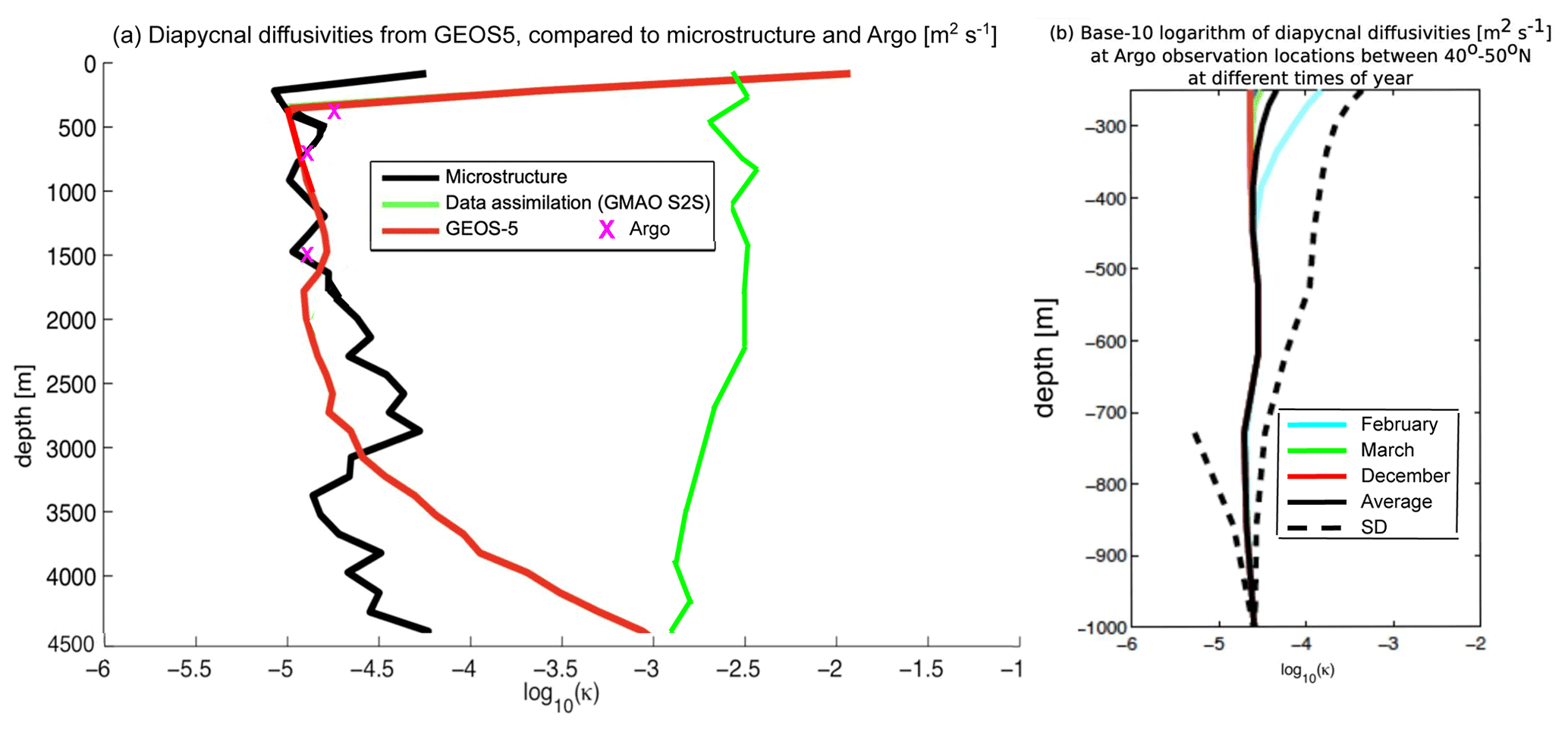
Figure A1 κ_ρ profiles (panel a; units in m² s⁻¹) averaged over the full-depth microstructure locations from the observations (black curve) presented in Waterhouse et al. (2014) (see their Fig. 6), the Whalen et al. (2015) Argo-derived product for three depth bins (magenta X marks), the temporally averaged output of a free-running coupled Earth system model simulation (GEOS-5 – red curve), and the temporally averaged output of an equivalent run with data assimilation (GMAO S2S – green curve). Also shown are (panel b) κ_ρ profiles from the free-running GEOS-5 simulation averaged over 40–50^∘ N in the North Atlantic Ocean and averaged over all January months (lighter colors) and all December months (darker colors). The base-10 logarithms of the geometric averages are shown in each panel.

Figure A2 Shown are (a) the base-10 logarithms of the ratios of the time-averaged κ_ρ,GMAO to κ_ρ,Argo and (b) the base-10 logarithms of the ratios of the time-averaged κ_ρ,GEOS5 to κ_ρ,Argo. Each panels shows an average over 250–2000 m depth. White areas in the ocean indicate insufficient Argo data to derive κ_ρ,Argo. The green X marks indicate regions where the disagreement between κ_ρ,GMAO or κ_ρ,GEOS5 and κ_ρ,Argo is greater than a factor of 3.

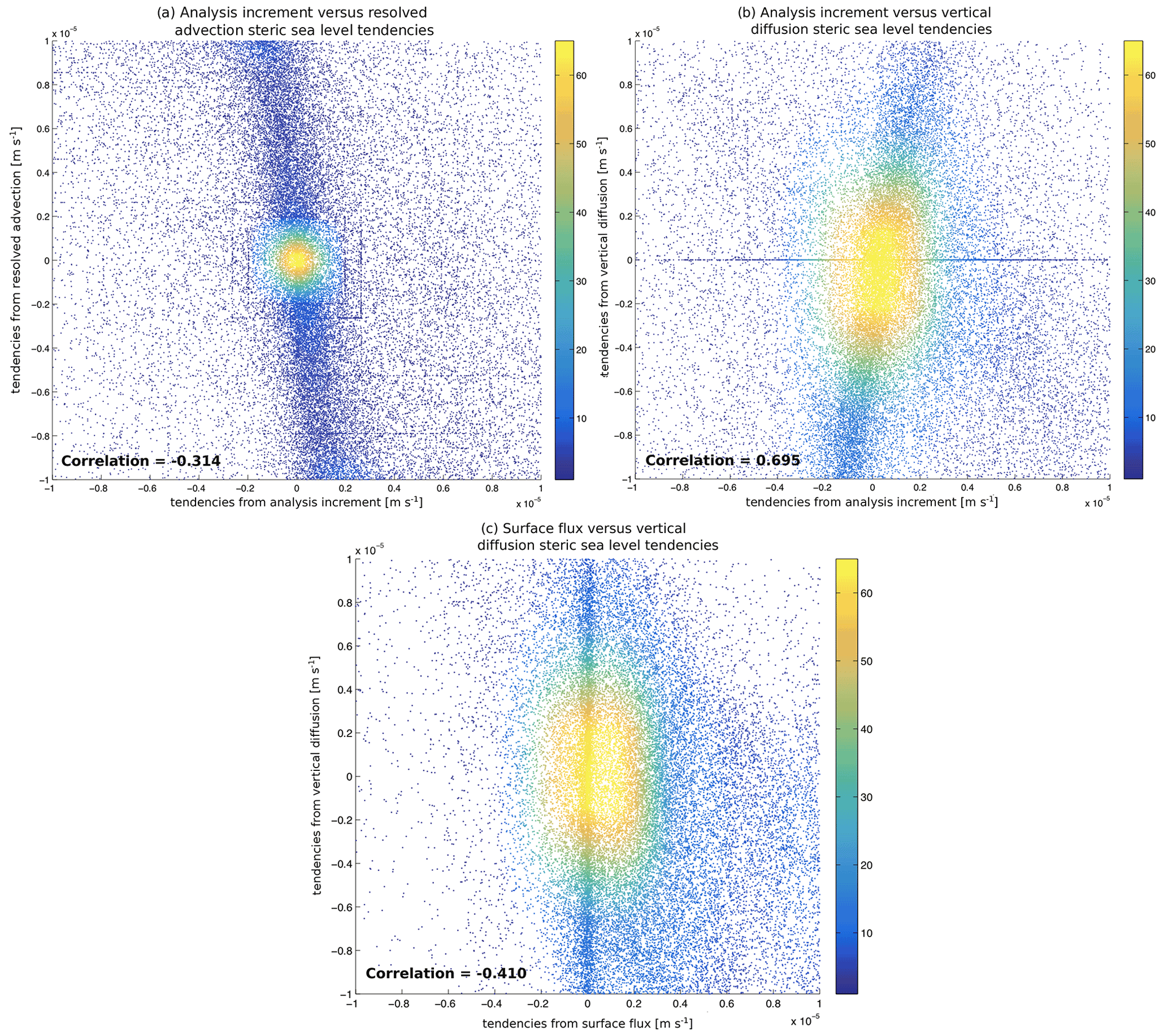
Figure A3 Scatterplots between several of the most locally dominant tendency terms in the steric sea level budget of the GMAO S2S Ocean Analysis, averaged over the entire runtime period (2012–2017): shown are (panel a) the analysis increment (abscissa) versus the resolved advection (ordinate) terms, (panel b) the analysis increment (abscissa) versus the vertical diffusion (ordinate) terms, and (panel c) the surface flux (abscissa) versus the vertical diffusion (ordinate) terms. The more yellow colors indicate a greater density of dots in the scatterplots. The more blue colors indicate a lower density of dots in the scatterplots. Also listed in each panel are the correlations between each of the comparisons.

The heat and salt budget terms summarized by Eq. (A1) are computed as follows. The resolved, mesoscale, and submesoscale transports are accounted for in the material derivatives Θ and S, the neutral and diapycnal diffusion of Θ and S is accounted for by J^Θ and J^S, and the analysis increments of Θ and S are accounted for by A^Θ and A^S. The neutral diffusion term includes cabbeling, thermobaricity, and a dianeutral contribution that mixes properties by providing for the exponential transition to horizontal diffusion in regions of steep isoneutral slopes according to Treguier (1992) and Ferrari et al. (2008, 2010) where the surface boundary layer is encountered and following Gerdes et al. (1990) next to solid walls. The diapycnal diffusion term is not added to the vertical component of the along-isopycnal diffusion term but because of convention (e.g., Palter et al., 2014) is nevertheless referred to as the vertical diffusion term hereafter. The vertical diffusion term also includes penetrating shortwave radiation flux. The sources and sinks of Θ and S accounted for by Q^Θ and Q^S include nonlocal convection (the transport for which turbulent fluxes do not depend upon local gradients in Θ or S because buoyant water gets entrained into the mixed layer when the surface buoyancy forcing drives convection above a stratified water column), surface buoyancy fluxes (latent, sensible, shortwave, longwave, and frazil heat fluxes), precipitation minus evaporation, runoff mixing (mixes properties associated with river outflows); downslope mixing (mixes properties downslope to represent the overflow of dense waters from marginal seas), sigma diffusion (mixing properties along terrain-following coordinates in regions with partial bottom cells), numerical smoothing of the free surface (intended to reduce B-grid checkerboard noise), numerical sponge (intended to absorb the Kelvin waves set off by the assimilation of some data), calving of land ice, and frazil ice formation. The runoff mixing, downslope mixing, and sigma diffusion terms are considered sources or sinks here because they are associated with numerical schemes that aim to resolve problems created by coarse model resolution, the vertical coordinate system used near boundary layers, and imperfect bathymetry. There is no geothermal heating included in the GMAO S2S Ocean Analysis. The vertical diffusion term includes a subsurface shortwave heating contribution to a function of the κ_ρ field, the mesoscale transport term assumes constant Gent–McWilliams coefficients, and the neutral diffusion term assumes constant Redi coefficients.

At each time step, the model evaluates a tendency term for every process that contributes to Eq. (A1) from their parameterized or dynamically calculated values, their units are converted to W m⁻² and $\mathrm{kg}{\mathrm{m}}^{-\mathrm{2}}{\mathrm{s}}^{-\mathrm{1}}$ for Θ and S, and their monthly averages are saved to the output files used in this analysis. Implicit in these output tendency terms is that each term is weighted by the thicknesses of each layer as the model runs and writes the output to file. The heat and salt budget terms saved to file are used to calculate the steric sea level budget as follows. The steric sea level budget terms are computed by scaling the heat tendency terms by $\mathit{\alpha }/C_p$ and the salt tendency terms by −1000β, where C_p (units in $\mathrm{J}{\mathrm{kg}}^{-\mathrm{1}}{\mathrm{K}}^{-\mathrm{1}}$) is the specific heat of seawater, $\mathit{\alpha }=-[\mathrm{1}/\mathit{\rho }](\partial \mathit{\rho }/\partial T)$ (units in K⁻¹) is the thermal expansion coefficient, and $\mathit{\beta }=[\mathrm{1}/\mathit{\rho }](\partial \mathit{\rho }/\partial S)$ (units in kg g⁻¹) is the haline contraction coefficient. In order to get a longitude–latitude map of the terms that depend upon depth shown here, we integrate over depth by summing over the depth dimension. We analyze part of the steric sea level budget of the GMAO S2S Ocean Analysis to examine the relationships between different terms.

Appendix B: Results for the sequential data assimilation framework

B1 Assessments of κ_ρ from models

First, we compare the average κ_ρ,micro profile that is comprised of data from 24 campaigns (Waterhouse et al., 2014) (see their Fig. 6; black curve in Fig. A1a) with the average model-calculated κ_ρ profiles and κ_ρ,Argo. A geometric average is taken for each profile because a geometric average is more representative than an arithmetic average for a small sample size and when the data are not normally distributed (Manikandan, 2011), like the lognormal distribution of κ_ρ (Whalen, 2021).

We compare microstructure (black curve in Fig. A1a) with GEOS-5 (red curve in Fig. A1a). κ_ρ,GEOS5, on average, is in close agreement with microstructure over the upper 250–2000 m. On average, the disagreement with microstructure and Argo is approximately the same as the disagreement between microstructure and GEOS-5. All three κ_ρ values are well within the uncertainty of the Argo product. The profiles are also within the temporal variability in κ_ρ,GEOS5 below the mixed layer depths (Fig. A1b; also see Fig. 9 in Whalen et al., 2015). The temporal variability in κ_ρ is only large near regions with active deep convection (e.g., between 40 and 50^∘ N in the North Atlantic Ocean, as shown in Fig. A1b). The blue and green diamonds in Fig. 1c of Waterhouse et al. (2014) show that there are only a few microstructure profiles are within the 40–50^∘ N band in the North Atlantic Ocean. These are all near the east coast of North America and not in regions that experience deep convection, so the temporal variability in microstructure is not expected to be large enough that the disagreements in κ_ρ can be explain by temporal sampling and/or aliasing.

While the average κ_ρ,GEOS5 profile is fairly accurate, particularly below 500 m depth (red curve in Fig. A1), κ_ρ,GMAO is in much worse agreement with microstructure (green curves in Fig. A1). The large values of κ_ρ,GMAO are not due to a few isolated locations. κ_ρ,GMAO is too large below about 250 m depth (solid green curve in Fig. A1). The average profile of κ_ρ,GMAO is generally constant or decreases with depth, as opposed to the average profiles of κ_ρ,GEOS5 and microstructure, which generally increase with depth. Potential reasons for the large disagreements between κ_ρ,GMAO and microstructure include dynamical adjustments due to the GMAO S2S Ocean Analysis increments, inconsistencies between the model's atmosphere and ocean due to the strong relaxation to sea surface temperatures, fixed zero net water input for global sea level, and numerics such as the techniques applied to damp the waves created from assimilating some observations.

B2 Model- vs. fine-scale parameterization-derived κ_ρ comparisons

While comparisons with microstructure reveal general agreement with the average profile of κ_ρ,GEOS5 – except near the surface and at deep depths – we also want to assess whether there are deficiencies in the average geographic distribution of κ_ρ,GEOS5 by comparing the output of GEOS-5 with the κ_ρ,Argo product. Comparing the κ_ρ,GEOS5 field with the κ_ρ,Argo product results in better agreement than the similar comparisons between κ_ρ,GMAO and κ_ρ,Argo. For example, κ_ρ,GEOS5 only disagrees with κ_ρ,Argo by more than a factor of 3 over 36.6 % of grid points with available data (Fig. A2b), while the disagreement doubles in percentage (79.1 %) for κ_ρ,GMAO (Fig. A2a). The errors in κ_ρ,GEOS5 are smaller than κ_ρ,GMAO. Thus, when the objective of the GMAO S2S Ocean Analysis is to minimize the misfit between the model and observations of temperature, salinity, and some surface characteristics, κ_ρ can be better represented without any observational constraints; i.e., the GMAO S2S Ocean Analysis improves temperature and salinity misfits for the wrong reasons.

The regions with the largest disagreement between κ_ρ,GEOS5 and κ_ρ,Argo are along the Equator, in the Southern Ocean, in the Labrador and Irminger seas, and in the Gulf Stream and Kuroshio extensions (Fig. A2b). Along the Equator the values of κ_ρ,GEOS5 tend to be larger than the observational product, but the discrepancy changes sign slightly poleward in the tropics near the Equator. Inadequate resolution and parameterization of diapycnal mixing can cause too little mixing to occur in these regions as well as in the Southern Ocean and along mid-ocean ridges (MacKinnon et al., 2017). The values of κ_ρ,GEOS5 are smaller than the observations both in regions where deep convection is prevalent and in the vicinity of the Antarctic Circumpolar Current (ACC). In the Gulf Stream Extension region, the Malvinas Current region, part of the Kuroshio Extension region, and the Indian Ocean sector of the ACC above 500 m depth, the values of κ_ρ,GEOS5 are too large. This is because κ_ρ,GEOS5 can be greatly increased inside the mixed layer depth, which can be deeper than 250 m due to vertical convection. One possible source of these errors in the abyssal κ_ρ is the improper treatment of remote internal tide-induced mixing, discussed in Melet et al. (2016), but several other processes can impact κ_ρ in the upper water column. For example, the wind-driven nearly inertial waves (Alford et al., 2016) can be important near the surface in many locations, and internal tide breaking is important near the seafloor at low latitudes in the Northern Hemisphere (Arbic et al., 2004; Nycander, 2005; Melet et al., 2013; MacKinnon et al., 2017) and beneath the ACC, where lee wave breaking is important (Nikurashin and Ferrari, 2011; Scott et al., 2011; Naveira Garabato et al., 2013; Melet et al., 2014; Wright et al., 2014; Trossman et al., 2013, 2016; Yang et al., 2018). MacKinnon et al. (2017) discuss other candidates for more accurate representation of κ_ρ. Identifying the sources of errors in κ_ρ,GEOS5, particularly in the abyss, is beyond the scope of the present study. We emphasize the much greater errors in κ_ρ,GMAO and next examine whether the analysis increments could be one source of these larger errors (either directly or by way of altering the velocity field).

B3 Relationships between steric sea level budget terms

There are distortions in temperature and salinity fields from applying analysis increments, violating conservation principles and potentially causing the model to undergo baroclinic adjustment (Stammer et al., 2016). Thus, we examine whether the velocity field itself changes because of the analysis increments. To do this, we show the relationship between the analysis increments and resolved advection terms in the steric sea level budget for the GMAO S2S Ocean Analysis in Fig. A3a. The Pearson correlation coefficient between the analysis increments and resolved advection terms in the steric sea level budget is about −0.3. The magnitudes of the analysis increments are determined by the temperature, salinity, and sea surface height fields, and the analysis increments and the resolved advection term in the GMAO S2S Ocean Analysis are comparable in size for both heat and salt tendencies – the largest terms in each budget in their zonal averages at most latitudes. However, previous studies have shown that analysis increments induce changes in the velocity field via dynamic adjustment (Stammer et al., 2016; Pilo et al., 2018). The correlation between the analysis increments and resolved advection terms shown in Fig. A3a is consistent with the findings of these previous studies. The analysis increments, by a similar argument, could induce physically inconsistent air–sea exchanges through changing the temperature and salinity fields in the top model layer. We next show that these factors at least partially cause errors in κ_ρ,GMAO. The Pearson correlation coefficients between the diapycnal diffusion terms and the analysis increment terms in the heat and salt budgets over all locations are about 0.7 (Fig. A3b), suggesting that the analysis increments are associated with errors in κ_ρ,GMAO. Problems with the physical consistency of air–sea exchanges – due to relaxation of sea surface temperatures and requiring net zero water input – could also contribute to the errors in κ_ρ,GMAO. However, it is possible that instead of the air–sea exchanges impacting the diapycnal diffusivities directly, the analysis increments affect both the air–sea exchanges and diapycnal diffusivities, as the changes in temperature and salinity at depth also change the mixed layer depths, which perturb the diapycnal diffusivity profiles and therefore their contribution to steric sea level through the altered thermal expansion and/or haline contraction coefficients. The surface flux and diapycnal diffusion terms in the heat and salt tendency budgets are fairly well-correlated with a Pearson correlation coefficient of about −0.4 (Fig. A3c), suggesting that there is an association between the surface flux errors and errors in κ_ρ,GMAO. Given these correlations and the way analysis increments and physical inconsistencies of air–sea exchanges are implemented in the GMAO S2S Ocean Analysis, errors in κ_ρ,GMAO must be caused by analysis increments (and possibly adjustments of air–sea exchanges) rather than the other way around.