Currents generated by the sea breeze in the southern Caspian Sea

The sea breeze system is the dominant atmospheric forcing at high frequency in the southern Caspian Sea. Here, we describe and interpret current meter observations on the continental margins of the southern Caspian from 2012 to 2013 to identify and characterize the water column's response to the sea breeze system. Time series analysis provides evidence for diurnal baroclinic current signals of O(0.02 m s⁻¹) and surface height changes of O(0.03 m). A two-layer model, including interfacial and bottom friction, is developed to further investigate the sea breeze response. This model is able to reproduce the structure, amplitudes, and phases of observed diurnal current fluctuations, explaining half of the variance in observational current response at frequencies at 1 cpd and higher. The sea breeze response thus results in a “tide-like” daily cycle, which is actually linked to the local forcing all along the southern Caspian coast.

1 Introduction

Diurnal-period onshore to offshore wind variability is a persistent feature of many coastal areas, especially in tropical and subtropical areas, but also in temperate zones (Sonu et al., 1973; Simpson, 1994; Steyn, 1998). Due to the smaller thermal heat capacity of land, it heats more rapidly in the day and cools more rapidly at night relative to the sea, resulting in land–sea thermal gradients with a daily cycle. This leads to cross-shore pressure gradients which generate onshore to offshore wind flows, called sea breeze systems, with the same daily periodicity. The diurnal sea breeze system can have a significant impact on the incident wave climate, nearshore processes, and morphology in tropical and subtropical regions (Sonu et al., 1973; Masselink and Pattiaratchi, 2001). Coastal currents can also be generated (Hyder et al., 2002; Zhang et al., 2009; Sobarzo et al., 2010; Gallop et al., 2012). These coastal currents can dominate the high-frequency variability over continental shelves (DiMarco et al., 2000; Rippeth et al., 2002; Hyder et al., 2002; Simpson et al., 2002). However, it is often difficult to separate tidal, inertial, and sea breeze effects in the coastal ocean response, since the timescales are very similar.

Recently, it was found that the variability of shelf currents in the southern Caspian Sea (Fig. 1a) is mostly dominated by coastally trapped waves with timescales of several days or longer (Masoud et al., 2019) but a significant daily signal is also present. The Caspian Sea, about 1030 km long and 310 km wide, is the largest enclosed basin in the world, and the southern coast, which is characterized by a shallow shelf of width 10–30 km with a deeper basin offshore, has a very persistent sea breeze pattern that is present through most of the year. Meteorological aspects of this pattern have been well-studied (Khoshhal, 1997; Azizi et al., 2010; Karimi et al., 2016), and analysis of a short current record at one station suggested that this sea breeze was linked to high-frequency variations in water column currents (Ghaffari and Chegini, 2010). Further, since tides in the Caspian Sea are very weak (Medvedev et al., 2016, 2017, 2020), it is possible that most of the higher-frequency variations in coastal currents may be a response to the sea breeze system.

Figure 1 (a) Southern Caspian Sea with the location of current meter moorings. Topography above and below the levels of the Caspian is derived from the ETOPO2 dataset (National Geophysical Data Center, 2001); the water level in the Caspian Sea is 28 m b.m.s.l. (below mean sea level). (b) Wind roses for total winds at mooring locations (Anzali and Noshahr roses are shifted southwards for clarity). (c) Wind roses for diurnal band-passed winds. Rings appear at 2 %, 4 %, and 6%.

Here, we take advantage of the strong and persistent sea breeze forcing in the southern Caspian Sea and the lack of confounding tidal effects, as well as the availability of measured current records at five well-separated locations along the southern Caspian shelf obtained between late 2012 and late 2013, to investigate the nature of a geophysical water column response on a shelf to periodic sea breezes. We find that the water column response to the sea breeze is measurable and widespread, occurring over the entire southern Caspian shelf year-round. However, the coupling between the atmosphere and ocean is a strongly local phenomenon, with changes in the timing of the daily cycle of currents responding to changes in the timing of the cycle of winds directly overhead, with no sign of propagation effects alongshore (unlike the case for lower-frequency current variations). Analytical solutions to a new coupled two-layer rotating wind-driven shallow-water model are compared with observations and show good agreement. Model dynamics also explain the nature of the local response.

1.1 The study area

The Caspian Sea (Fig. 1a) is a terminal basin into which rivers flow but water is only lost by evaporation; its surface is about 28 m below mean ocean level. Although the northern Caspian Sea is very shallow, with depths of less than 50 m, the southern part is characterized by a central region with depths of more than 800 m, bordered on the south and west by a narrow shelf area (Fig. 1) extending 10–30 km offshore to the 100 m isobath. Inshore of this is a coastal plain of varying width, backed up by the Alborz mountains with heights of up to 5610 m. On the southeastern coast, the shelf extends offshore more than 100 km; the coastal plain there is similarly flat and extends well inland.

Most of the fresh water enters from the Volga River in Russia to the north. There are many small rivers on the southern (Iranian) coast, but together they supply only 5 % of the freshwater input (Alizadeh et al., 2008). The large-scale stratification in the Caspian's water column varies seasonally, with warm salty (20–30 ^∘C, 12 PSU) waters in a relatively well-mixed layer about 40–100 m deep in summer and fresher, less warm (10 ^∘C, 11 PSU) surface waters in winter (Zaker et al., 2007) above more stratified waters at depth. However, even within this mixed layer there is often a weak stratification.

Atmospheric forcing governs the mostly cyclonic mean circulation of the Caspian Sea, but winds are generally weak in the southern Caspian with mean speeds of only 3–4 m s⁻¹; wind speeds are less than 5 m s⁻¹ more than 90 % of the time (Kosarev, 2005). The occasional strong winds along the southern Caspian coast result in the formation of baroclinic coastally trapped waves along the shelf edge (Masoud et al., 2019). These waves propagate from west to east at speeds of 1–3 m s⁻¹ and explain most of the variance in currents at frequencies less than 1 cpd.

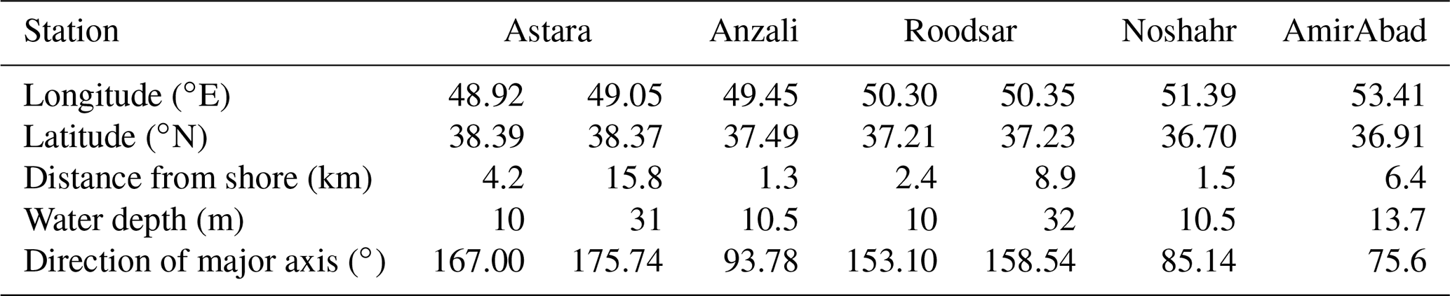
Table 1 Location, water depth, and distance to shore for all mooring locations. Also given is the direction of the principal axis of current variations. The details of ADCPs located in deeper water are presented in the second column for Astara and Roodsar.

The southern Caspian has a humid subtropical climate characterized by warm summers and mild winters, and it receives a significant amount of solar radiation (Kosarev, 2005). At higher frequencies the sea breeze is then an important phenomenon which exists throughout the year but is most widespread in spring and summer months (Khoshhal, 1997; Azizi et al., 2010; Ghaffari and Chegini, 2010; Karimi et al., 2016). A typical sea breeze in warm months is generated by solar radiation. However, in other months when the temperature gradient between the sea and land surfaces is low, other mechanisms, for example outflows from the Alborz mountains in winter known as Garmesh winds, can also increase temperatures in the coastal plain, generating a sea breeze (Khoshhal, 1997; Karimi et al., 2016).

A typical sea breeze cycle in the southern Caspian is characterized by onshore winds (the “sea breeze”) generally starting more than 2 h after sunrise at around 9:00–noon (see, e.g., Azizi et al., 2010; Ghaffari and Chegini, 2010; Karimi et al., 2016, all times referred to here are in local summer time, which is known as Iran Daylight Time – IRDT – or UTC+4:30). The wind direction changes to offshore (the “land breeze”) around 16:00–21:00. The maximum wind speed of about 4 m s⁻¹ occurs during the sea breeze between noon and 16:00 after the time of maximum temperature gradient between sea and land. The strongest and most frequent sea breeze days occur in areas around AmirAbad and Anzali where the coastal plain is widest, and the fewest sea breeze days are observed around Noshahr and Astara (Azizi et al., 2010; Karimi et al., 2016).

1.1.1 Data and data processing

The wind and current meter datasets used here were fully described in Masoud et al. (2019), and only brief details are given here. Over a period of about 16 months from late 2012 to early 2014, current velocity measurements using 600 kHz Nortek AWAC acoustic Doppler current profilers (ADCPs) were collected at five locations a few kilometers offshore in depths of about 10 m over the southern Caspian shelf in successive monthly deployments (Fig. 1 and Table 1). Measurements for the period of December 2012 to December 2013, when spatial and temporal coverage was most complete, are used here. More sparse information is also available at two locations further offshore near the 30 m isobath at Astara and Roodsar. The instruments used collected data every 10 min with a vertical bin resolution of 0.5 m; the lowest useful bin, which we use to show bottom currents, is 2 m above the bottom.

Some local observations of surface winds are available at three stations (Anzali, Noshahr, and AmirAbad) out of our five stations during 2013, but even these data contain gaps. So for consistency we use winds at 10 m above the water surface, which are extracted from a Weather Research and Forecasting (WRF) model configured for the Caspian Sea region, interpolated to the location of ADCP measurement stations. The WRF model, described at length in Bohluly et al. (2018), is configured with two nests. The 42×52 outer domain has a resolution of 0.3^∘, and the 94×124 inner domain grid has a resolution of 0.1^∘. The 6-hourly ERA-Interim reanalysis data from the European Centre for Medium-Range Weather Forecasts (ECMWF) are used as initial and boundary conditions. The model is run daily starting at 18:00 for 1.25 d with 6 h of spin-up time that is discarded. The accuracy of modeled winds has been evaluated by Bohluly et al. (2018) and Ghader et al. (2014). The latter compared model winds with a variety of observed wind products over the Caspian Sea including one offshore buoy, three nearshore buoys, and also data from the QuikSCAT satellite product. Qualitative and quantitative assessment of these comparisons showed that the simulated surface wind fields are in good agreement with the observational data and QuikSCAT satellite data. We also evaluated the accuracy of the WRF wind data ourselves by comparing with available wind buoy data at three locations during 2013 (the wind data are available mostly between May and September). The root mean square error (RMSE) between WRF wind and observed wind is less than 0.1, 0.11, and 0.2 m s⁻¹ at Anzali, Noshahr, and AmirAbad, respectively. The wind stress is calculated from the 10 m elevation wind velocity from the WRF model using drag coefficients from Large and Pond (1981). Since the WRF model is run on a daily cycle, the diurnal peaks in the spectra that we describe later could be numerical artifacts. However, similarly strong diurnal peaks are observed in spectra of observed wind from buoy data at Anzali and AmirAbad and from land stations located near Astara, Anzali, Noshahr, and AmirAbad stations (not shown), so we believe the WRF outputs reflect real conditions. In addition, the daily analysis we perform in this paper starts at midnight, and hence any systematic forecast-to-forecast step would occur at figure boundaries.

Finally, water levels in the southern Caspian are measured by tide gauges at Anzali (37.48^∘ N, 49.46^∘ E) and at AmirAbad (36.85^∘ N, 53.37^∘ E). For our purposes (to see daily variations) we subtract the daily mean from each day. This removes any biases resulting from a seasonal cycle with a range of about 0.4 m, as well as long-term trends.

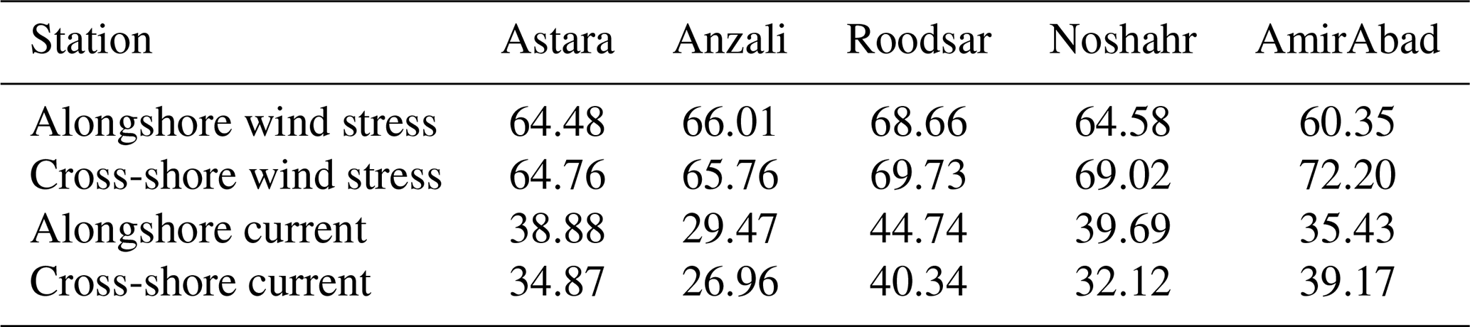
Table 2 Ratio of diurnal variance (band-passed filter with removing periods less than 6 h and more than 30 h) to high-frequency variance (frequencies higher than 1 cpd) for alongshore and cross-shore wind stress and bottom current. Ratios are in percentage.

2 Results

2.1 Total and diurnal-period winds

Wind roses at our five study sites (Fig. 1b) show that winds are generally aligned along the coast, with maximum wind speeds of about 10 m s⁻¹. However, if we separate out the diurnal variability using a Butterworth fourth-order band-pass filter to remove periods less than 6 h and more than 30 h, wind roses for this band-limited time series show mostly cross-shelf variation with speeds of up to 4 m s⁻¹ at three stations. Diurnal winds at the other two (Astara and Noshahr) still have a significant alongshore component (Fig. 1c). Astara is at the southern end of a large inland plain from which sea breezes are generated, so the sea breeze will align with the coast, and the coastal plain is also very narrow at Noshahr, making it difficult to generate a large cross-shore wind.

Subtracting the mean, the wind stress and current data are then rotated based on principal axes of the currents at 4 m to align with the local bathymetry so that vectors are decomposed into alongshore and cross-shore components (Table 1, Fig. 2). The diurnal wind stress represents about 60 %–72 % of the high-frequency wind stress variability, depending on location (Table 2), and the diurnal current variability represents about 27 %–45 % of the high-frequency current variability near the bottom.

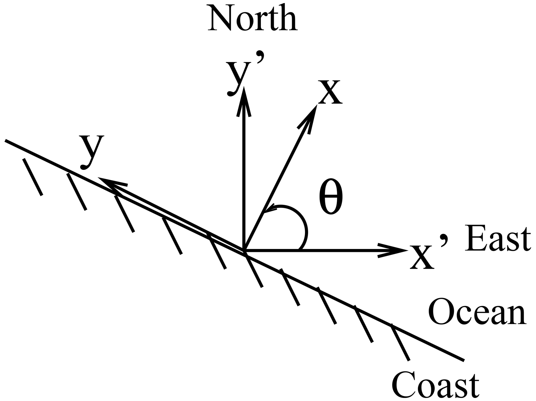
Figure 2 Definition of axes. Offshore direction is the positive x axis; θ is the rotation angle between geographic and coastal axes.

2.1.1 Wind and current spectra

Wind stress spectra have a narrow, statistically significant spectral peak at 1 cpd at all stations (Fig. 3a and c); it is strongest at Roodsar. There is both clockwise and anticlockwise motion in diurnal frequencies, although the clockwise motion is stronger everywhere except at AmirAbad, consistent with the strong directionality of the daily wind rose there (Fig. 1c) and generally clockwise rotations elsewhere. Smaller spectral peaks also occur at the first harmonic of the diurnal frequency (frequencies of ±2 cpd) at many stations and sometimes (e.g., at AmirAbad) at higher harmonics as well.

Rotary spectra for bottom currents also have narrow, statistically significant peaks at 1 cpd and small peaks at the first harmonic frequencies (Fig. 3b and d). Spectra for wind and currents computed for each season rather than for the whole year (not shown here) also contain the 1 cpd peak. Although these peaks are always present they are largest in the summer and spring. At frequencies higher than about 2 cpd, wind stress spectra continue to slope downwards, whereas bottom current spectra begin to flatten. This suggests that the current time series is mostly dominated by instrument white noise at these high frequencies. We shall then restrict our analysis to frequencies less than 2 cpd.

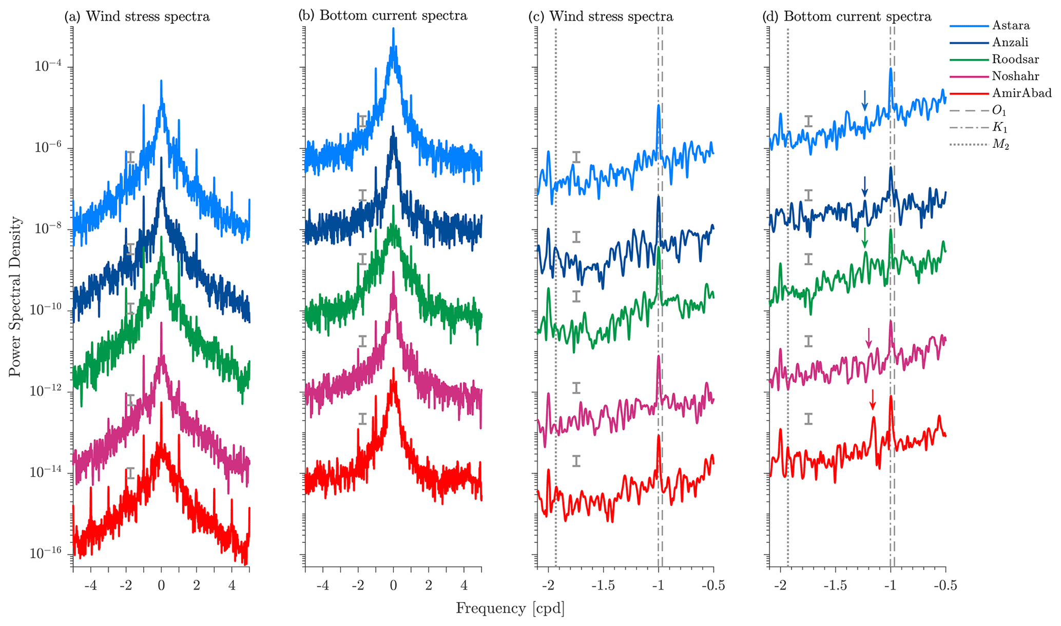
Figure 3 Rotary power spectral density estimates of (a) wind stress and (b) bottom current at Astara, Anzali, Roodsar, Noshahr, and AmirAbad stations using the Welch method. Successive spectra are offset downwards by 100 N m² cpd⁻¹ for wind stress and 100 m² s⁻² cpd⁻¹ for currents. Negative and positive frequencies correspond to clockwise and counterclockwise rotation, respectively. The grey error bars indicate 95% confidence intervals. (c) A magnification of the wind stress spectra for clockwise diurnal frequencies. (d) The same for bottom currents. The arrows indicate the inertial frequency (at approximately 1.2 cpd) at each station, and other vertical grey lines mark the location of the O₁ (0.9295 cpd), K₁ (1.0027 cpd), and M₂ (1.9323 cpd) tidal frequencies.

Inertial frequencies, which at around 1.2 cpd at these latitudes are well-separated from the diurnal frequency, are associated with a very weak peak in bottom currents at most locations (Fig. 3d). Although we cannot separate the diurnal peak from any that might be associated with the dominant diurnal tidal constituent (K₁), there is clearly no visible peak at the frequency of the next most important diurnal constituent (O₁) or at the frequency of the dominant semi-diurnal constituent (M₂), strongly suggesting that the diurnal and semi-diurnal peaks represent a response to wind stress forcing at those frequencies and not tidal variability.

2.1.2 The sea breeze

In order to concentrate our attention on the sea breeze forcing and response, ignoring the low-frequency variability which was discussed in Masoud et al. (2019), we will analyze only band-passed data (removing data with periods less than 6 h and more than 30 h) from now on. Examining a 4 d period typical of the summer (Fig. 4i), the daily cycle of the sea breeze system is obvious, with onshore wind (the sea breeze) in the late morning–early afternoon and offshore wind (the land breeze) in the night–early morning. Winds rotate in the clockwise direction. The daily cycle of band-passed wind directions for the whole study period demonstrates the predominance of this daily change from onshore to offshore wind (Fig. 5) over the whole year. At all locations the wind blows onshore in the early afternoon, starting at about 5 h after sunrise (even as the time of sunrise varies over the year), and the onshore direction changes to offshore around sunset, remaining in that direction until late morning (Figs. 4i and 5).

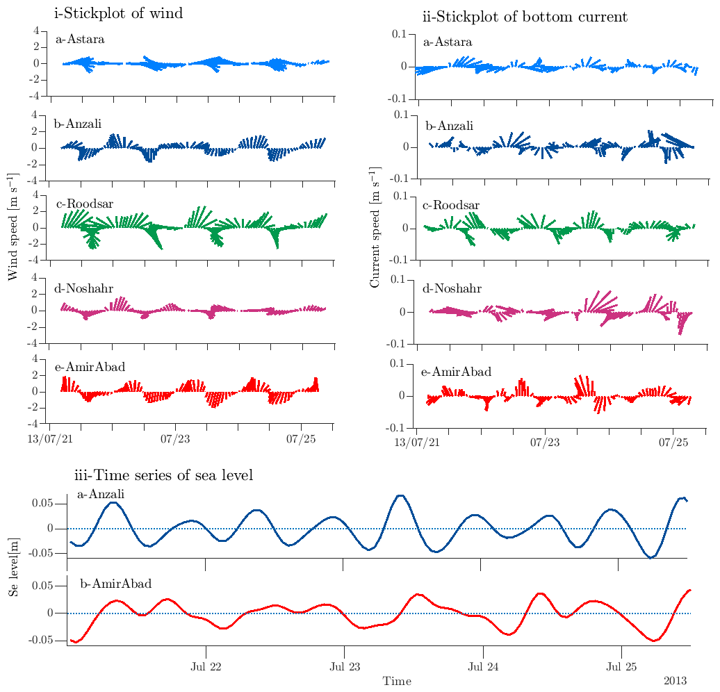
Figure 4 An example of summer daily variability from 21–25 July 2013. (i) Stick plot of hourly band-passed alongshore and cross-shore winds at (a) Astara, (b) Anzali, (c) Roodsar, (d) Noshahr, and (e) AmirAbad. In this figure the coastline is horizontal with water above and land below; positive upwards (positive y) winds in the morning are offshore, and negative downward (negative y) winds in the afternoon are onshore. (ii) Stick plot of band-passed alongshore and cross-shore current at (a) Astara, (b) Anzali, (c) Roodsar, (d) Noshahr, and (e) AmirAbad. (iii) Time series of sea level at (a) Anzali and (b) AmirAbad.

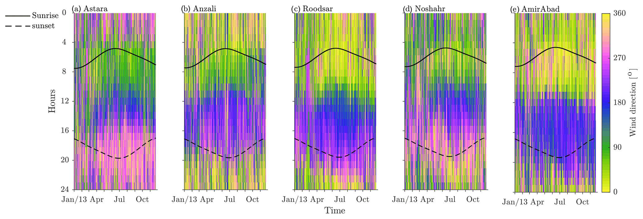
Figure 5 Wind direction at (a) Astara, (b) Anzali, (c) Roodsar, (d) Noshahr, and (e) AmirAbad. Angles increase clockwise from the offshore direction so that a wind direction of $\mathrm{0}/\mathrm{360}$^∘ is pure offshore wind and 180^∘ is pure onshore wind. The black solid and dashed lines are sunrise time and sunset times, respectively (Beauducel, 2021).

The diurnal bottom currents are slightly less consistent from day to day (Fig. 4ii) but show an onshore current in the mornings and offshore currents in the evenings. Although these currents also mostly turn clockwise, they are not in phase with the winds, and their magnitude varies over the whole year (not shown) from less than 0.01 m s⁻¹ to as much as 0.2 m s⁻¹ on occasion.

More quantitatively, we count the number of sea breeze days at all locations using a standard algorithm applied to our band-passed datasets. In most selection methods for sea breeze days, the diurnal reversal of wind direction from offshore to onshore is used as an identifier for a sea breeze day (Masselink and Pattiaratchi, 2001; Furberg et al., 2002; Miller and Keim, 2003; Azorin-Molina and Chen, 2009). Additionally, a rapid change in the intensity of wind is considered in some cases. Here, a sea breeze day is counted when (1) the wind direction during the day (from 10:00 to 23:00) is from the sea breeze direction (onshore) but the wind overnight (from 23:00 to 10:00) is not from the same direction (greater than 60^∘ wind direction difference) and (2) the wind directions in the afternoon and morning are both from the sea breeze direction (onshore) but afternoon (noon to 23:00) wind speed is larger than wind speed in the morning (10:00 to noon).

Using these selection criteria, about 220–280 sea breeze days occur in 2013 depending on the location, with a mean wind speed of 1.5 m s⁻¹ (Fig. 6). The most are seen at Roodsar (which also has the strongest winds) and the fewest at Astara. However, sea breeze activity is subject to a slight seasonal variability. In spring and summer (April–September), approximately 20–30 sea breeze days are experienced every month. However, closer to 10–25 sea breeze days occur per month in fall and winter seasons (October–March).

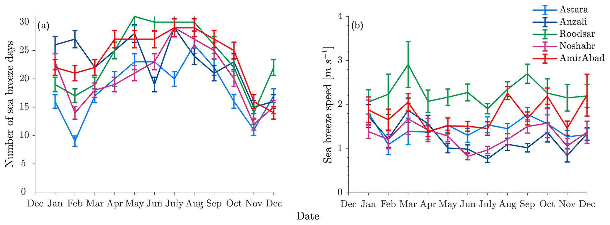
Figure 6 (a) Number of sea breeze days and (b) sea breeze speed at Astara, Anzali, Roodsar, Noshahr, and AmirAbad stations for each month from December 2012 to December 2013.

Water level measurements (Fig. 4iii) are available at two locations. The daily range is about 0.1 m at both. At AmirAbad there is a “low” water level around noon and a high water level a few hours after midnight. There is additionally a larger twice-a-day signal at Anzali. If we perform a tidal harmonic analysis using T_Tide (Pawlowicz et al., 2002), we find M₂ tidal amplitudes of 0.02 and 0.007 m for Anzali and AmirAbad stations, respectively. O₁ amplitudes are below the noise level, but S₁ amplitudes, at 0.01 and 0.03 m for Anzali and AmirAbad, respectively, are significantly larger than their close neighbors P₁ and K₁. S₂ is also substantial. However, Medvedev et al. (2016), examining water level records in the central Caspian, suggest that the anomalously large S₁ and S₂ constituents actually represent “radiational” tides, probably resulting from the sea breeze. The narrowness of these spectral peaks is then a result of the extremely consistent sea breeze pattern over the whole year.

2.1.3 The mean diurnal cycle

Now we consider an “average” day. Although the annual changes in sunrise and sunset times result in a slight annual modulation in the timing of the sea breeze (Fig. 5), we ignore this variation and average by hour of the day over the whole year. We also processed the data using only the deduced “sea breeze” days, but find the smaller number of days in the mean gave more variable results than averaging over the whole year; the sea breeze day selection algorithm appears to be overly conservative.

The resulting time series of daily wind stress (Fig. 7) again shows the same general pattern at all stations, but demonstrates a little more clearly how the magnitude of the signal, and the relative strengths of cross-shore and alongshore wind stresses, varies from place. Alongshore winds are to the right in the morning and to the left (when facing offshore) in the afternoon and evening. These winds are strongest at Roodsar and weakest at Anzali. The daily cycle is not a pure sinusoid but contains distortions associated with higher harmonics. These are greatest at AmirAbad, consistent with the appearance of wind spectra (Fig.  3). In addition, there are more subtle differences in the timing of peaks and transitions. For example, the transition from offshore to onshore flow occurs as early as 9:00 at Noshahr but as late as 11:00 at Roodsar. The transition back to offshore flow occurs at 16:00 at Noshahr and Astara but as late as 23:00 at Roodsar and AmirAbad.

Figure 7 The 24 h averaged daily cycle of band-passed alongshore and cross-shore wind stress (first panel), as well as the alongshore current (second panel) and cross-shore current (third panel) at (a) Astara, (b) Anzali, (c) Roodsar, (d) Noshahr, and (e) AmirAbad stations from December 2012 to December 2013. The current data are band-passed and then averaged by hours; we remove values from bins that are too close to the surface and (at AmirAbad) bins with unstable averages.

In the water column, the average diurnal cycle is similarly uniform in its patterns at all locations, although the magnitude and exact timing of the cycle also vary from place to place (Fig. 7). The cross-shore currents are almost entirely baroclinic, with a node at a height above bottom of around 6 to 7.7 m, a short distance above the middle of the water column (Fig. 7iii). Although we do not have measurements close to the bottom or surface due to limitations imposed by the ADCP design, it seems likely that this pattern consists of the first baroclinic mode and that surface currents are coherent with, but even larger than, those seen in the topmost bin for which reasonable averages can be obtained. After midnight, there is an offshore flow in the surface layer, apparently matching the offshore wind stress, and onshore flow at the bottom layer. An opposite pattern with an onshore flow in the surface layer (and an onshore wind stress) and offshore flow at the bottom layer can be observed during daylight hours. The magnitude of the average cycle is O(0.01 m s⁻¹), which is largest at Roodsar and Astara and smaller at the other three locations. Oscillation peaks, as well as peaks in the offshore wind stress, occur slightly later at Roodsar and AmirAbad relative to the other stations. These delays do not consistently trend eastwards or westwards and hence do not suggest alongshore propagation of wave-like features.

The alongshore cycle is also quite similar at all stations (Fig. 7). Here, however, a noticeable barotropic flow can be seen, in addition to a baroclinic pattern. Current maximums and minimums of O(0.01 m s⁻¹) near the bottom lag those at the surface by about $\mathrm{1}/\mathrm{4}$ wave period so that they reach a maximum while surface values approach zero (and vice versa). In the diurnal alongshore current pattern, there is a negative (rightward) flow in the daytime and positive (leftward) flow in the nighttime.

The stronger winds at Roodsar and Astara are correlated with stronger currents, and weaker winds at Anzali and Noshahr are associated with weaker currents. The timing of changes in the direction of winds and the timing of changes in the direction of currents, which do vary slightly from location to location, are also linked; locations with later peaks and zero crossings in wind stress time series also have later peaks and zero crossings in current time series. There is therefore a high (local) correlation between the sea breeze system and the diurnal currents all along the southern Caspian coast.

In addition to the moorings at depths of ∼10 m, two additional current meter moorings at Astara and Roodsar were also located further offshore at the 31 and 32 m isobath (Table 1). Although no useful data were returned from the upper half of the water column there, the daily cycles of currents in the lower half (Fig. 8) are similar in direction, magnitude, and timing to those seen at the bottom in the shallower locations, and there also weak indications at the shallowest depth for which reliable measurements can be obtained that an upper layer is present with flows similar to the upper layer flow in shallower waters. Thus, daily oscillations in both surface and bottom waters, with similar pattern and timing, are probably present in the water column over wide areas of the shelf.

Figure 8 The 24 h averaged daily cycle of band-passed alongshore wind stress and cross-shore wind stress (first panel), as well as the alongshore current (second panel) and cross-shore current (third panel) for (a) Astara at 31 m and (b) Roodsar at 32 m (Table 1).

2.2 Theoretical water column response to the sea breeze

To further understand the linkages between the diurnal surface wind stress and the diurnal currents, we now attempt to model the dynamics. Instead of following the depth-dependent “oscillating Ekman layer” approach of Craig (1989b) with a vertical eddy viscosity coupled to a barotropic mode, which has been used by many authors, we restrict ourselves to a mathematically simpler coupled two-layer system, as suggested by our observations, for which analytical solutions are more straightforward to obtain.

Thus, consider a linearized two-layer shallow-water model on the semi-infinite plane bounded by a coastline on the y axis, with the positive x axis pointed offshore (Fig. 2) into shelf waters of depth H_T≈10 m (numerical values for these and other parameters are presented here without comment to justify the mathematical development; we shall discuss their origin in the next section). Since we are considering a local response over scales of the shelf width, we will filter out long shelf waves (which in any case are not suggested by our observations at daily frequencies) by assuming negligible variation in the alongshore direction, but we retain the possibility of an alongshore wind stress. Also, since the mooring locations are well inshore of the shelf break and energy that propagates across the shelf break will not return, we can neglect the increase in depth past the shelf break. The upper layer of undisturbed depth H₁≈3.5–6 m is then governed by

$$\begin{array}{}\text{(1)}& {\displaystyle }& {\displaystyle }{u}_{\mathrm{1}t}-f{v}_{\mathrm{1}}=-g{\mathit{\eta }}_{\mathrm{1}x}+{\displaystyle \frac{{\mathit{\tau }}^{\left(x\right)}}{\mathit{\rho }{H}_{\mathrm{1}}}}-{\displaystyle \frac{r}{H_{\mathrm{1}}}}\left(u_{\mathrm{1}}-u_{\mathrm{2}}\right)-R{u}_{\mathrm{1}},\text{(2)}& {\displaystyle }& {\displaystyle }{v}_{\mathrm{1}t}+f{u}_{\mathrm{1}}={\displaystyle \frac{{\mathit{\tau }}^{\left(y\right)}}{\mathit{\rho }{H}_{\mathrm{1}}}}-{\displaystyle \frac{r}{H_{\mathrm{1}}}}\left(v_{\mathrm{1}}-v_{\mathrm{2}}\right)-R{v}_{\mathrm{1}},\text{(3)}& {\displaystyle }& {\displaystyle }{\left({\mathit{\eta }}_{\mathrm{1}}-{\mathit{\eta }}_{\mathrm{2}}\right)}_t+H_{\mathrm{1}}{u}_{\mathrm{1}x}=\mathrm{0},\end{array}$$

and the lower layer of undisturbed depth H₂≈6.5 m is governed by

$$\begin{array}{}\text{(4)}& {\displaystyle }& {\displaystyle }{u}_{\mathrm{2}t}-f{v}_{\mathrm{2}}=-g{\left[(\mathrm{1}-\mathit{\epsilon }){\mathit{\eta }}_{\mathrm{1}}+\mathit{\epsilon }{\mathit{\eta }}_{\mathrm{2}}\right]}_x-{\displaystyle \frac{r}{H_{\mathrm{2}}}}\left(u_{\mathrm{2}}-u_{\mathrm{1}}\right)-R{u}_{\mathrm{2}},\text{(5)}& {\displaystyle }& {\displaystyle }{v}_{\mathrm{2}t}+f{u}_{\mathrm{2}}=-{\displaystyle \frac{r}{H_{\mathrm{2}}}}\left(v_{\mathrm{2}}-v_{\mathrm{1}}\right)-R{v}_{\mathrm{2}},\text{(6)}& {\displaystyle }& {\displaystyle }{\mathit{\eta }}_{\mathrm{2}t}+H_{\mathrm{2}}{u}_{\mathrm{2}x}=\mathrm{0},\end{array}$$

with g the gravitational acceleration, (u_i, v_i) velocities and H_i layer depths for the upper (i=1) and lower (i=2) layers, $\mathit{\epsilon }=({\mathit{\rho }}_{\mathrm{2}}-{\mathit{\rho }}_{\mathrm{1}})/\mathit{\rho }\approx \mathrm{2}\times {\mathrm{10}}^{-\mathrm{4}}$ (with ρ_i layer densities and ρ a reference density), and τ^(x) and τ^(y) applied wind stresses in the offshore and alongshore directions. In this set of equations, r is an interfacial friction, and R represents a bottom friction, both characterized by their timescales r⁻¹ and R⁻¹, respectively. We (somewhat inconsistently) include R in both the upper and lower layer equations since this allows us to completely separate the baroclinic and barotropic modes next. The equations for each layer are fully coupled by the appearance of the interface height η₂ in both, as well as by the interfacial friction; wind stress affects only the surface layer. The coastline boundary condition is that $u_{\mathrm{1}}=u_{\mathrm{2}}=\mathrm{0}$ at x=0.

Using procedures described in Sect. 16 of LeBlond and Mysak (1981), these six coupled equations can be approximately separated into two independent sets of three equations each when ε≪1. A barotropic mode for which

$$\begin{array}{}\text{(7)}& u_{\mathrm{1}}=u_{\mathrm{2}}\mathrm{and}{\mathit{\eta }}_{\mathrm{1}}={\displaystyle \frac{H_{\mathrm{1}}+H_{\mathrm{2}}}{H_{\mathrm{1}}}}{\mathit{\eta }}_{\mathrm{2}},\end{array}$$

implying that the two interfaces move together in the same direction with about the same magnitude and that currents are the same from top to bottom, is then governed by the following equations.

$$\begin{array}{}\text{(8)}& {\displaystyle }& {\displaystyle }{u}_t-fv=-g{\mathit{\eta }}_x+{\displaystyle \frac{{\mathit{\tau }}^{\left(x\right)}}{\mathit{\rho }{H}_T}}-Ru\text{(9)}& {\displaystyle }& {\displaystyle }{v}_t+fu={\displaystyle \frac{{\mathit{\tau }}^{\left(y\right)}}{\mathit{\rho }{H}_T}}-Rv\text{(10)}& {\displaystyle }& {\displaystyle }{\mathit{\eta }}_t+H_T{u}_x=\mathrm{0}\end{array}$$

where

$$\begin{array}{}\text{(11)}& {\displaystyle }& {\displaystyle }u\approx {\displaystyle \frac{H_{\mathrm{1}}{u}_{\mathrm{1}}+H_{\mathrm{2}}{u}_{\mathrm{2}}}{H_T}}\text{(12)}& {\displaystyle }& {\displaystyle }\mathit{\eta }\approx {\mathit{\eta }}_{\mathrm{1}}\text{(13)}& {\displaystyle }& {\displaystyle }{H}_T\approx H_{\mathrm{1}}+H_{\mathrm{2}}\end{array}$$

Thus, this mode is mostly linked to sea surface height variations. The intrinsic speed of high-frequency waves is $\sqrt{g{H}_T}\approx \mathrm{10}$ m s⁻¹.

In addition, there is also a separate baroclinic mode for which

$$\begin{array}{}\text{(14)}& u_{\mathrm{2}}=-{\displaystyle \frac{H_{\mathrm{1}}}{H_{\mathrm{2}}}}{u}_{\mathrm{1}}\mathrm{and}{\mathit{\eta }}_{\mathrm{1}}=-\mathit{\epsilon }{\displaystyle \frac{H_{\mathrm{2}}}{H_{\mathrm{1}}+H_{\mathrm{2}}}}{\mathit{\eta }}_{\mathrm{2}},\end{array}$$

governed by

$$\begin{array}{}\text{(15)}& {\displaystyle }& {\displaystyle }{u}_t-fv=-g\mathit{\epsilon }{\mathit{\eta }}_x+{\displaystyle \frac{{\mathit{\tau }}^{\left(x\right)}}{\mathit{\rho }{H}_{\mathrm{1}}}}-\left({\displaystyle \frac{r}{H^{\prime }}}+R\right)u,\text{(16)}& {\displaystyle }& {\displaystyle }{v}_t+fu={\displaystyle \frac{{\mathit{\tau }}^{\left(y\right)}}{\mathit{\rho }{H}_{\mathrm{1}}}}-\left({\displaystyle \frac{r}{H^{\prime }}}+R\right)v,\text{(17)}& {\displaystyle }& {\displaystyle }{\mathit{\eta }}_t+H^{\prime }{u}_x=\mathrm{0},\end{array}$$

where

$$\begin{array}{}\text{(18)}& {\displaystyle }& {\displaystyle }u\approx u_{\mathrm{1}}-u_{\mathrm{2}},\text{(19)}& {\displaystyle }& {\displaystyle }\mathit{\eta }\approx -{\mathit{\eta }}_{\mathrm{2}},\text{(20)}& {\displaystyle }& {\displaystyle }{H}^{\prime }\approx {\displaystyle \frac{H_{\mathrm{1}}{H}_{\mathrm{2}}}{H_{\mathrm{1}}+H_{\mathrm{2}}}},\end{array}$$

which implies that for this mode, velocity shear is linked to mid-water interface depth changes (which are far larger than the associated surface height changes), and high-frequency interface displacements travel with an intrinsic speed of $\sqrt{g\mathit{\epsilon }{H}^{\prime }}\approx \mathrm{0.07}$ m s⁻¹, much slower than for the barotropic mode. More importantly, the friction for the baroclinic mode must be greater than or equal to that affecting the barotropic mode, but the forcing stress is also larger (see changes in denominator of the wind stress terms).

Now, we wish to find the response of this system to a known diurnally oscillating (and possibly rotating) wind stress. Fortunately, the equations governing both the barotropic and baroclinic modes are almost identical, albeit with coefficients whose numerical values are different so that the same analytic solution can easily be adapted for either. For simplicity, let us consider a canonical set of equations as follows.

$$\begin{array}{}\text{(21)}& \begin{array}{rl}& u_t-fv=-g{\mathit{\eta }}_x+T^{\left(x\right)}-r^{\prime }u\\ & v_t+fu=T^{\left(y\right)}-r^{\prime }v\\ & {\mathit{\eta }}_t+H{u}_x=\mathrm{0}\end{array}\end{array}$$

Now assume that both alongshore and cross-shore wind stress vectors decay offshore with a length scale α⁻¹ (≈100 km) and are oscillatory with a daily-frequency ω modeled by the real part of

$$\begin{array}{}\text{(22)}& T^{\left(x\right)}=T_{\mathrm{0}}^{\left(x\right)}{e}^{-\mathit{\alpha }x-i\mathit{\omega }t}\mathrm{and}{T}^{\left(y\right)}=T_{\mathrm{0}}^{\left(y\right)}{e}^{-\mathit{\alpha }x-i\mathit{\omega }t}\end{array}$$

for constants $T_{\mathrm{0}}^{\left(x\right)}$ and $T_{\mathrm{0}}^{\left(y\right)}$.

We look for solutions that vanish as x⟶∞. The total solution is made of a particular solution to the forced problem and a homogeneous solution to the unforced equations, which are added together to match the coastal boundary condition. For the particular solution, we guess that u, v, and η will also decay offshore with a scale α⁻¹ and oscillate with a frequency ω:

$$\begin{array}{}\text{(23)}& u=U_p{e}^{-\mathit{\alpha }x-i\mathit{\omega }t},v=V_p{e}^{-\mathit{\alpha }x-i\mathit{\omega }t},\mathit{\eta }=N_p{e}^{-\mathit{\alpha }x-i\mathit{\omega }t},\end{array}$$

where it is implicit in this approach that we take only the real part of the final (complex) solution. A nondimensional decay scale, $\mathit{\sigma }=r^{\prime }/\mathit{\omega }$ (which we will find to be ≈0 for the barotropic mode but ∼1 for the baroclinic mode), is defined to consider frictional effects. The particular solution then satisfies

$$\begin{array}{}\text{(24)}& {\displaystyle }& {\displaystyle }-i\mathit{\omega }(\mathrm{1}+i\mathit{\sigma })U_p-f{V}_p=g\mathit{\alpha }{N}_p+T_{\mathrm{0}}^{\left(x\right)},\text{(25)}& {\displaystyle }& {\displaystyle }-i\mathit{\omega }(\mathrm{1}+i\mathit{\sigma })V_p+f{U}_p=T_{\mathrm{0}}^{\left(y\right)},\text{(26)}& {\displaystyle }& {\displaystyle }-i\mathit{\omega }{N}_p-H\mathit{\alpha }{U}_p=\mathrm{0},\end{array}$$

whose solution for horizontal velocities in matrix form is

$$\begin{array}{}\text{(27)}& \begin{array}{rl}\left[\begin{array}{c}{U}_p\\ V_p\end{array}\right]& ={\displaystyle \frac{\mathrm{1}}{\mathit{\beta }}}\cdot \left[\begin{array}{cc}i\mathit{\omega }(\mathrm{1}+i\mathit{\sigma })& -f\\ f& i\mathit{\omega }\left\{(\mathrm{1}+i\mathit{\sigma })+\frac{gH{\mathit{\alpha }}^{\mathrm{2}}}{{\mathit{\omega }}^{\mathrm{2}}}\right\}\end{array}\right]\\ & \cdot \left[\begin{array}{c}{T}_{\mathrm{0}}^{\left(x\right)}\\ T_{\mathrm{0}}^{\left(y\right)}\end{array}\right],\end{array}\end{array}$$

where

$$\begin{array}{}\text{(28)}& \mathit{\beta }={\mathit{\omega }}^{\mathrm{2}}(\mathrm{1}+i\mathit{\sigma }{)}^{\mathrm{2}}-f^{\mathrm{2}}+gH{\mathit{\alpha }}^{\mathrm{2}}(\mathrm{1}+i\mathit{\sigma }),\end{array}$$

with the height linked to offshore velocities through

$$\begin{array}{}\text{(29)}& N_p={\displaystyle \frac{iH\mathit{\alpha }}{\mathit{\omega }}}{U}_p.\end{array}$$

For the homogeneous problem, a wave-like solution is considered:

$$\begin{array}{}\text{(30)}& u=U{e}^{ikx-i\mathit{\omega }t},v=V{e}^{ikx-i\mathit{\omega }t},\mathit{\eta }=N{e}^{ikx-i\mathit{\omega }t},\end{array}$$

leading to a dispersion relation of

$$\begin{array}{}\text{(31)}& k^{\mathrm{2}}={\displaystyle \frac{{\mathit{\omega }}^{\mathrm{2}}(\mathrm{1}+i\mathit{\sigma })-f^{\mathrm{2}}/(\mathrm{1}+i\mathit{\sigma })}{gH}}\end{array}$$

as well as

$$\begin{array}{}\text{(32)}& V={\displaystyle \frac{fU}{i\mathit{\omega }(\mathrm{1}+i\mathit{\sigma })}}\end{array}$$

and

$$\begin{array}{}\text{(33)}& N={\displaystyle \frac{kHU}{\mathit{\omega }}}.\end{array}$$

Although in the inviscid limit there are free waves propagating offshore (real k) for frequencies above the inertial frequency and evanescent waves (i.e., imaginary k with solutions decaying exponentially in x) at lower frequencies, as will be the case in the Caspian, once friction is significant then k will be complex. Here we have decay scales of $Im\mathit{\{}k{\mathit{\}}}^{-\mathrm{1}}\approx \mathrm{200}$ km for the barotropic mode and around 1 km for the baroclinic mode. We can also (by combining with Eq. 28) write

$$\begin{array}{}\text{(34)}& \mathit{\beta }=gH\left({\mathit{\alpha }}^{\mathrm{2}}+k^{\mathrm{2}}\right)(\mathrm{1}+i\mathit{\sigma })\end{array}$$

which shows that α will have little effect on the magnitude of the baroclinic response, although it will be important for the barotropic response, including water level at the coast. Friction will directly affect both, but possibly in a complicated way, since the 1+iσ term also appears in the numerator for some terms in Eq. (27).

Adding the particular and homogeneous solutions and setting $U=-U_p$ to meet the coastal boundary condition $u(x=\mathrm{0})=\mathrm{0}$, the complete response is given by

$$\begin{array}{}\text{(35)}& {\displaystyle }& {\displaystyle }u=U_p\left\{e^{-\mathit{\alpha }x}-e^{ikx}\right\}{e}^{-i\mathit{\omega }t},\text{(36)}& {\displaystyle }& {\displaystyle }v=V_p\left\{e^{-\mathit{\alpha }x}-{\displaystyle \frac{f{U}_p}{(i\mathit{\omega }-r^{\prime })V_p}}{e}^{ikx}\right\}{e}^{-i\mathit{\omega }t},\text{(37)}& {\displaystyle }& {\displaystyle }\mathit{\eta }={\displaystyle \frac{iH{U}_p}{\mathit{\omega }}}\left\{\mathit{\alpha }{e}^{-\mathit{\alpha }x}+ik{e}^{ikx}\right\}{e}^{-i\mathit{\omega }t},\end{array}$$

with U_p and V_p from Eq. (27).

Note that in the baroclinic case, the expressions within the braces will be dominated by the first term (except very near the coast) so that the baroclinic current magnitude and phase response will be similar everywhere on the shelf and will be of similar magnitude in both the along and cross-shore directions. However, for the barotropic case, the similarity of α and Im{k} means that the cross-shore barotropic current response will be very small and may be much smaller than the alongshore barotropic response. These conclusions about relative amplitudes are in general accord with our observations (Fig. 8).

From our observations, we have both cross-shore and alongshore winds of similar magnitude, and in this case it becomes difficult to generalize further about the relationships between currents and the wind stress. Thus, for further analysis we now try and tune the predicted response to our observations by first matching the measured daily wind cycle (i.e., finding $T_{\mathrm{0}}^{\left(x\right)}$ and $T_{\mathrm{0}}^{\left(y\right)}$ specifically for each location) and then, by taking the offshore distances and layer heights from our observations, adjusting the offshore decay scale α⁻¹ and frictions R and r as global parameters to match the observations.

2.2.1 Fitting of model to data

Fitting sinusoids with a period of 1 d to the daily wind stress time series to estimate $T_{\mathrm{0}}^{\left(y\right)}$ and $T_{\mathrm{0}}^{\left(y\right)}$ for each location is straightforward (Fig. 9i), as these time series are clearly dominated by the daily variations with only a small amount of energy in the higher harmonics, as we have seen earlier (Fig. 3). However, the lack of ADCP data near the surface results in some difficulty in separating the barotropic and baroclinic modes in the water column observations. The layer interface is evident from the baroclinic response in Fig. 7 at about 6–7.7 m above the bottom at different stations, and this is not centered in the depth range for which observed velocities ${\stackrel{\mathrm{‾}}{u}}_{\mathrm{o}}=(u_{\mathrm{o}},v_{\mathrm{o}})$ are available. Using this information as well as the surveyed total water depths (Table 1), we take layer heights in pairs of (4, 6), (3.5, 7), (3.5, 6.5), (4, 6.5), and (6, 7.7) for (surface, bottom) layer thicknesses at Astara, Anzali, Roodsar, Noshahr, and AmirAbad, respectively. Similarly we can take the offshore distances as observed from Table 1.

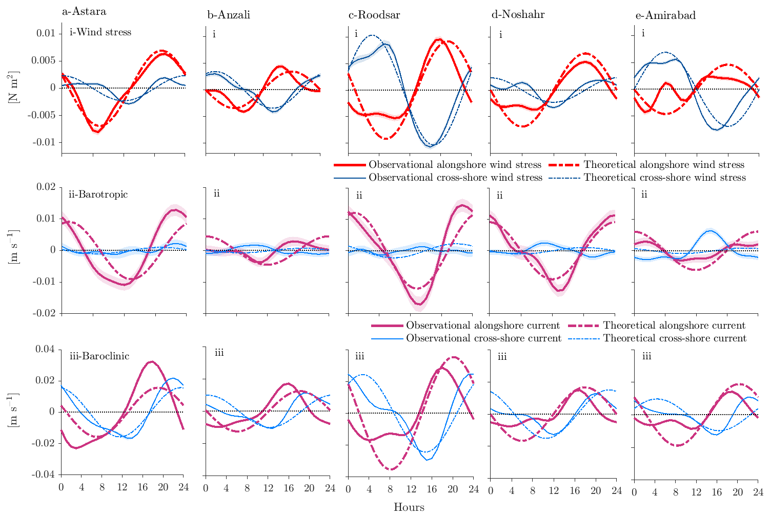
Figure 9 Mean daily cycle of (i) observed (solid line) and theoretical (dash–dot line) alongshore and cross-shore wind stress, (ii) observed (solid line) and theoretical (dash–dot line) barotropic alongshore and cross-shore current response, and (iii) observed (solid line) and theoretical (dash–dot line) alongshore and cross-shore baroclinic current response at (a) Astara, (b) Anzali, (c) Roodsar, (d) Noshahr, and (e) AmirAbad stations. The shading indicates the 95 % confidence level for the observed current data.

Next, we estimate the barotropic response by averaging observed current velocities ${\stackrel{\mathrm{‾}}{u}}_{\mathrm{o}}$ at equal distances above and below the apparent layer interface and the baroclinic response by subtracting current velocity at these depths (Fig. 9ii and iii). For example, if the interface was judged to be at 6 m,

$$\begin{array}{}\text{(38)}& \begin{array}{rl}& {\stackrel{\mathrm{‾}}{u}}_{\mathrm{barotropic}}={\displaystyle \frac{{\stackrel{\mathrm{‾}}{u}}_{\mathrm{o}}\left(\mathrm{8}\mathrm{m}\right)+{\stackrel{\mathrm{‾}}{u}}_{\mathrm{o}}\left(\mathrm{4}\mathrm{m}\right)}{\mathrm{2}}},\\ & {\stackrel{\mathrm{‾}}{u}}_{\mathrm{baroclinic}}={\stackrel{\mathrm{‾}}{u}}_{\mathrm{o}}\left(\mathrm{8}\mathrm{m}\right)-{\stackrel{\mathrm{‾}}{u}}_{\mathrm{o}}\left(\mathrm{4}\mathrm{m}\right).\end{array}\end{array}$$

The alongshore barotropic response is largest at Astara and Roodsar (Fig. 9ii), where alongshore winds are also largest. The cross-shore barotropic response is small compared to the alongshore barotropic response at all locations. In contrast, the alongshore and cross-shore baroclinic responses are similar in magnitude to each other at all stations (Fig. 9iii), although together they are strongest at Astara and Roodsar; the baroclinic response with peak values of O(0.02 m s⁻¹) is also about twice as large as the barotropic response.

Hydrographic profiling did not occur regularly during the current meter program, and although we have found some data the quality is rather low. Nevertheless, they do suggest that there may be a weak stratification over the shelf, and from this we very roughly estimate that the water column is characterized by a nondimensional density difference between layers of $\mathit{\epsilon }\approx \mathrm{2}\times {\mathrm{10}}^{-\mathrm{4}}$. Note, however, that the exact value of this parameter is not too important, as its main dynamical effect here (other than to ensure a baroclinic mode exists) is to set an the offshore decay scale for the effects of the coastal boundary. As long as ε is small, this response generally occurs only inshore of our mooring locations and hence will not affect the quality of our fits, nor will it have any effect on the response over the rest of the shelf offshore.

The offshore decay scale for the forcing α⁻¹ has been estimated to be about 150 km by comparing the energy magnitude in the diurnal peak of wind spectra at different locations offshore perpendicular to Anzali, Noshahr, and AmirAbad stations (1.5, 10, 40, 150, and 300 km). Changing α⁻¹ from 10 to 300 km has only a small impact on the phase shift and magnitude of the modeled baroclinic response, mostly near the shelf edge (not shown) as αx→1. However, the magnitude of the barotropic response (especially for cross-track velocity and the amplitude of surface height changes) does depend directly on α through its importance in the β factor (Eq. 28) as was discussed above.

The most sensitive tuning factor is then the friction. However, it too has only a limited ability to modify the solutions. Taking the phase and magnitude of winds for Roodsar, increasing friction from 0 to σ≈1 decreases the magnitude of the velocities for the barotropic mode (Fig. 10 left side) but causes virtually no difference in the phase of the barotropic cross-shore velocity. Increasing friction does result in a slight advance in the phase of the alongshore velocity and a slight delay in the phase of the surface height cycle. Its largest effect is in greatly decreasing the magnitude of the surface height change, halving it for σ≈1. Note that the alongshore velocity is similar at all locations across the shelf, and the cross-shore velocity is small but increases linearly with distance from the coast.

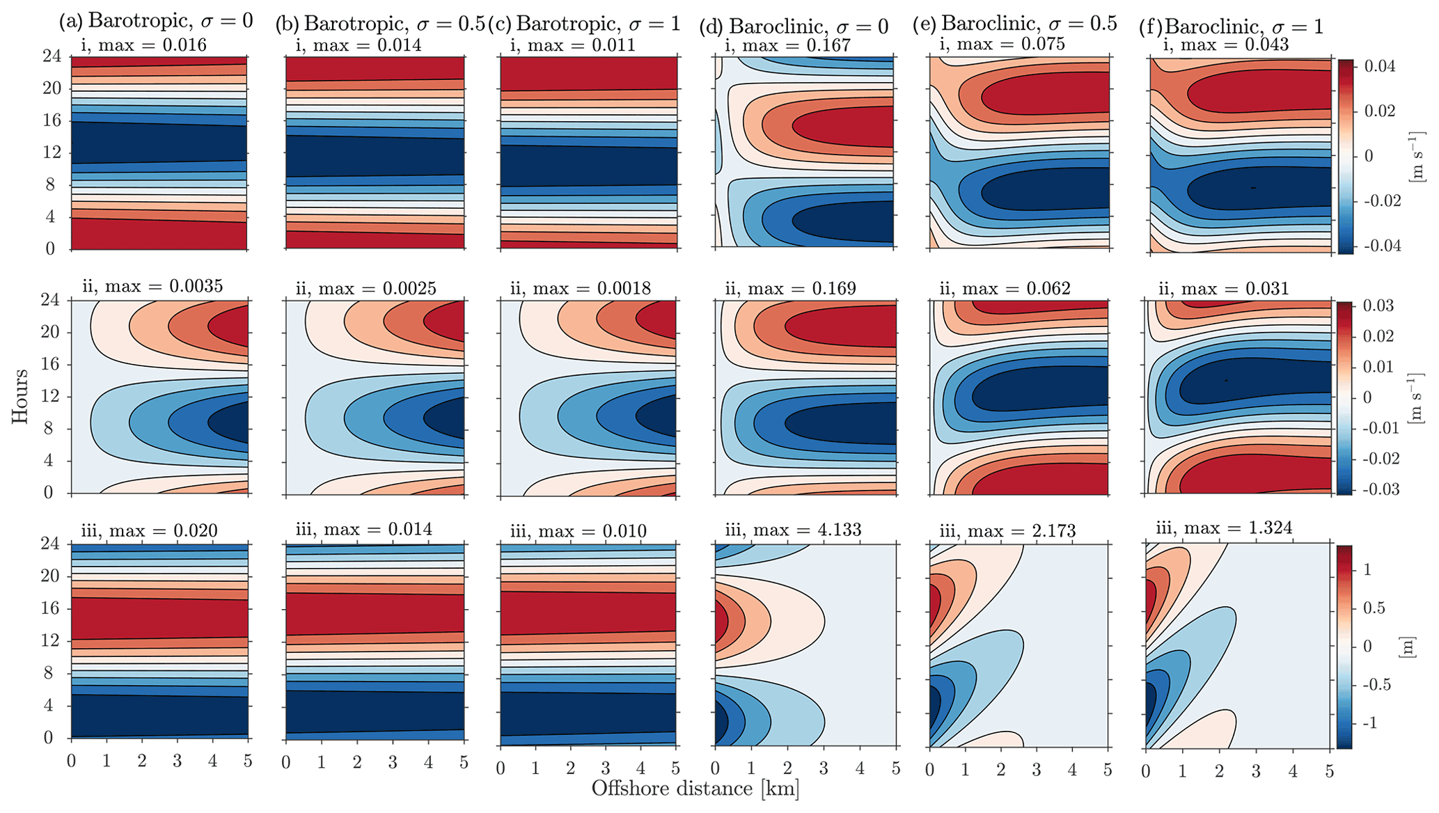
Figure 10 Sensitivity of alongshore current, cross-shore current, and sea level response to the friction parameter. Sensitivity of the modeled (a) barotropic response with σ=0, (b) barotropic response with σ=0.5, (c) barotropic response with σ=1, (d) baroclinic response with σ=0, (e) baroclinic response with σ=0.5, and (f) baroclinic response with σ=1 for (i) Alongshore current, (ii) cross-shore current, and (iii) sea level with $\mathit{\alpha }=\mathrm{1}/\mathrm{150}$ km⁻¹ at Roodsar station. The red and blue represent positive and negative values, respectively.

The baroclinic mode, on the other hand, has a velocity response which is far more sensitive to friction. Increasing friction to σ=1 reduces the velocity magnitudes to about $\mathrm{1}/\mathrm{4}$ of the inviscid values and significantly delays the phase by almost a quarter cycle. For very weak friction, both phase and amplitude are affected, but with larger σ∼1 the major effect is to reduce the amplitude. Alongshore and cross-shore velocities have similar magnitudes everywhere offshore. However, there are significant changes in the velocity amplitudes, phases, and interface heights very near the coast.

The barotropic response at all locations is then quite adequately matched by an inviscid (σ=0) barotropic mode (Fig. 9ii). Note that the barotropic response actually rotates counterclockwise, although this is difficult to see since the current ellipse is so narrow. The observed baroclinic response, on the other hand, is somewhat delayed relative to the inviscid solutions, and friction of σ=1 must be added to both capture this delay and match the observed amplitudes. The baroclinic response rotates in a clockwise direction.

Given the limited amount of tuning possible, the predicted responses are, in general, quite close to our observations in both amplitude and phase. In particular, the predicted amplitude and phase of barotropic alongshore current and baroclinic alongshore and cross-shore current are in reasonable agreement with the observations at all stations. However, the observed responses sometimes contain large departures from a daily sinusoid.

Finally, our model can also provide estimates of layer height changes. Observations of surface height are available at the coast near two of our locations. The observed “mean daily” cycle at these locations shows a range of about 0.02 m (Fig. 11) at all locations. Both the amplitude and phase of the sea-breeze-forced response are in reasonable agreement with these observations. Predicted mid-water interface height changes related to the baroclinic mode at our mooring locations offshore are actually slightly smaller than the surface height changes, making them difficult to discern in our observations since the vertical bin size in our measurements was 0.5 m. Although the amplitude of the modeled water level is in good agreement with the observed one in Anzali, the phase of the modeled response does not catch the semi-diurnal tidal component at this station.

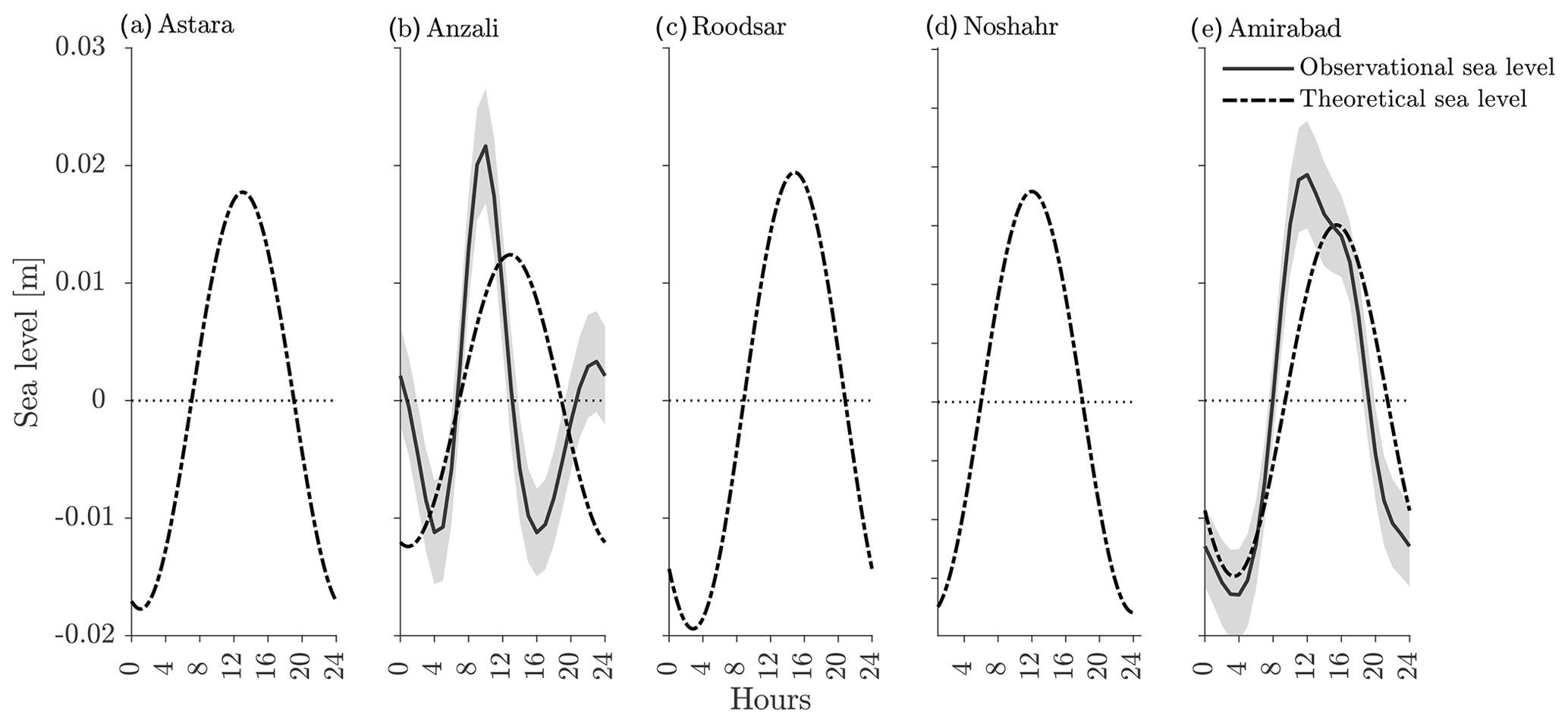
Figure 11 Mean daily cycle of observed water level (solid line) only at Anzali and AmirAbad stations and theoretical (dash–dot line) water level at (a) Astara, (b) Anzali, (c) Roodsar, (d) Noshahr, and (e) AmirAbad. The shading indicates the 95 % confidence level.

3 Discussion

In the southern Caspian Sea, the sea breeze system, with winds of up to 4 m s⁻¹ and wind stresses of up to about 0.02 N m⁻² (but on average peaking at 2 m s⁻¹ and less than 0.01 N m⁻²), is the major diurnal–inertial-period process in the atmosphere, explaining about two-thirds of high-frequency variance in winds (Table 2) and hence dominating the forcing of coastal processes at high frequency. Ghaffari and Chegini (2010) found that these winds were highly correlated with currents in the high-frequency range at a mooring west of AmirAbad and speculated that there was a link between the sea breeze system and high-frequency variance in currents. Anomalously large S₁ constituents in tidal analyses for coastal Caspian Sea water levels also suggest a noticeable radiational effect, which has in the past been ascribed to sea breezes (Medvedev et al., 2016). We find here that daily-frequency current variations of ±0.02 m s⁻¹ and daily surface height changes of about 0.03 m are clearly consistent with the water column response to the local sea breeze forcing all along the southern Caspian coast and that this response is seen year-round. In both the alongshore and cross-shore directions this daily response is large and baroclinic; there is also an alongshore barotropic component, which is about half as large, and an even smaller cross-shelf barotropic component linked to coastal water level changes.

In comparison, lower-frequency coastally trapped waves in the same area, generated by lower-frequency wind variations, are associated with rather larger barotropic current variations over the shelf (although they can have depth structure further offshore) of O(0.1 m s⁻¹), mostly in the along-shelf direction, and surface height changes of O(0.1 m), which are also larger than those for sea breeze (Masoud et al., 2019). Known processes that affect water level also include an annual cycle of magnitude O(0.4 m) due to seasonal imbalances between river inflow and evaporation, as well as astronomically forced tidal signals as large as 0.06 m (Medvedev et al., 2020). Thus, we conclude here that the water column response to the sea breeze does not dominate time series of currents, although it is clearly an important factor in short-term coastal water level changes, resulting in a small “tide-like” daily cycle. The sea breeze current response is, however, very consistent over time, and is therefore also clearly visible as distinct peaks in spectra of the currents (Fig. 3) and sea level (not shown), as well as in time series in which the lower-frequency motions are filtered away (Fig. 4).

If we require a band-passed wind speed to be greater than a particular threshold to be classified as a true sea breeze, as is typically done in sea breeze studies (Masselink and Pattiaratchi, 2001; Furberg et al., 2002; Miller and Keim, 2003; Azorin-Molina and Chen, 2009), we count more than 220 sea breeze days in 2013, with an average wind speed of 1.5 m s⁻¹ (Fig. 6). These details change from location to location but with average speeds at Roodsar about double the speeds at Noshahr and Anzali. In summer, more than 20 sea breezes occur monthly. Less frequent sea breeze days are observed in winter. On the other hand, time series of band-pass-filtered wind angle (Fig. 5) show that this daily reversal is present at nearly all times, although again the details of timing change from location to location.

Our findings for 2013 thus agree with earlier work in concluding that the atmospheric sea breeze is an obvious and featured phenomenon in the southern Caspian Sea area, especially in spring and summer months (Khoshhal, 1997; Azizi et al., 2010; Ghaffari and Chegini, 2010; Karimi et al., 2016). Also in agreement with this earlier work, we find that the sea breeze starts in late morning sometime between 9:00 and 11:00 (depending on time of year and location), reaches its maximum velocity between about 12:00–16:00, and subsides between 16:00–22:00, after which it is replaced by the land breeze (Figs. 4, 5 and 7i). This pattern of onshore sea breeze during the day followed by offshore winds at night, particularly in spring and summer, is a characteristic feature of many other coastal areas (Rosenfeld, 1988; DiMarco et al., 2000; Simpson et al., 2002; Hyder et al., 2002; Zhang et al., 2009; Sobarzo et al., 2010; Gallop et al., 2012); however, most of these other investigations were based on observations from only one or two (usually close together) locations. A significant result here is that the sea breeze system in the southern Caspian Sea and its water column response are shown to be coupled in a very similar way over a distance of about 500 km along a coastline, although the exact timing of both the forcing and the response does vary from place to place. By comparing phase at these different locations, we find that the variations are not consistent with a phase propagation along the coast, as was found at lower frequencies at which the eastward delays were associated with the passage of coastally trapped waves (Masoud et al., 2019). This suggests that the response to the widespread diurnal forcing is mostly local, which would be consistent with the evanescent (i.e., non-“wave-like”) nature of an oceanic forced response, as we are north of the critical latitude for daily variations.

Not only is a sea breeze seen along the coastline, but the offshore extent of the sea breeze was also estimated here to be 150 km. Although the typical scale of a sea breeze system is 50 km for subtropical areas described by Sonu et al. (1973), Simpson (1994), and Steyn (1998), other studies (Largier and Boyd, 2001; Simpson et al., 2002) reported the existence of strong diurnal oscillations on the outer Namibian shelf and at Benguela shelf edge. Significant diurnal winds extending to an offshore site 125 km from the coast of northern Africa at latitude 22^∘ N were reported (Halpern, 1977). Since the shelf area is only 10–30 km wide, the sea breeze thus affects the entire width of the shelf, and in turn the pattern of currents that arise in response to the sea breeze might also be expected to be similar over the shelf width, except perhaps very close to the coast where the response must adjust to the coastal “wall”.

In detail, the local water column response to the sea breeze can be described as follows: in the cross-shore direction, currents are baroclinic with a zero crossing near the middle of the water column (Fig. 7). The sea breeze forces onshore surface flow and offshore bottom flow during daytime, with the opposite at night. The total excursion for water parcels would be around 600 m. There is little barotropic offshore flow, although it cannot be zero since a small daily variation in surface height is seen at the coast, with lowest waters during daylight hours. Note that the baroclinic response is also weak enough that the mid-water interface also does not vary in height very much over most of the shelf. In contrast, the daily alongshore response is much more strongly barotropic, especially at Roodsar, with flow leftwards at night and rightwards (when facing offshore) in daytime, with a total excursion of about 300 m.

A diurnal current response to diurnal wind stress with a combined barotropic–baroclinic response in the alongshore direction and two-layer baroclinic structure in the cross-shore direction was also clearly observed on the Chilean shelf at 36–37^∘ S (Sobarzo et al., 2010). The flow in the surface layer was downwind, and the motion at the bottom layer was in the opposite direction. A baroclinic response has also been seen elsewhere at or poleward of the critical latitude (Hyder et al., 2002; Simpson et al., 2002; Rippeth et al., 2002; Sobarzo et al., 2010). A unique aspect of our observations is that diurnal bottom and surface currents have almost the same amplitude. In contrast, many previous studies have found that the diurnal surface current is stronger than the bottom current, and the amplitude of the oscillations in the bottom layer is weaker than in the surface layer, by a factor which is a function of the depth of the pycnocline (Rosenfeld, 1988; Rippeth et al., 2002; Hyder et al., 2002; Zhang et al., 2009; Sobarzo et al., 2010; Gallop et al., 2012). Here the stratification is weak enough that no distinct pycnocline exists on the shelf; instead the first baroclinic mode separates the water column into two almost equal layers.

Theoretical models of the circular motion and vertical structure of current response to diurnal winds in shallow and deep water in the presence of a coast, after the decay of transients, have been investigated by Craig (1989a, b). A one-dimensional, constant-density analytical model was applied with an assumption that the bottom layer flow is forced by the coast-normal pressure gradient due to the periodic wind stress, without considering frictional effects (Craig, 1989b). The mean flow is driven by a barotropic surface slope resulting from the applied wind stress. Simpson et al. (2002) examined numerical solutions including the effects of frictional coupling between layers, extending Craig's approach. Craig's analytical model has also been extended in a numerical solution to a multi-layer structure with frictional coupling between the layers via an eddy viscosity by Rippeth et al. (2002). In this model energy propagates down through the water column through frictional coupling of adjacent layers as in the classical Ekman problem. However, Rippeth et al. (2002) also used a two-layer analytical model without considering friction effects to demonstrate current response to wind in the diurnal band.

Here, our observations clearly suggest a two-layer response, without alongshore propagation of long waves, which is superimposed on lower-frequency variations arising from coastally trapped waves, so we have developed a new linear two-layer model, including interfacial and bottom friction but without alongshore variations, to investigate the sea breeze response and the important factors governing this response in a more general way. Analytical solutions that we develop for this forced system greatly simplify the identification of important factors in the response, without making prior judgments about their importance.

For the barotropic mode, bottom friction can reduce the magnitude of the response, but it has only minor effects on the phase. The magnitude of the response is also affected by α, so to some extent changes in either bottom friction or α can compensate for changes in the other. However, friction must remain weak as increasing friction advances the phase of the (strong) alongshore component and would hence reduce the agreement with the phase of observations. Previous modeling of low-frequency coastally trapped waves in the southern Caspian (Masoud et al., 2019) required a linear bottom friction of $\mathrm{1.5}\times {\mathrm{10}}^{-\mathrm{4}}$ m s⁻¹ to agree with observations. Spread out over the 10 m water column to agree with our formulation for friction this would be equivalent to $R=\mathrm{1.5}\times {\mathrm{10}}^{-\mathrm{5}}$ s⁻¹, which, for daily variations, would imply σ∼0.2; this is larger than any value that we might wish to use here. It is likely then that this large value represents scattering losses for previously studied alongshore wave propagation rather than truly frictional effects.

For the baroclinic mode, phase effects are larger, and an interfacial friction of σ=1 is clearly important for matching the observed baroclinic response. Similarly, Hyder et al. (2002) inferred a relatively large linear friction coefficient (σ≈0.6) to match the phase difference between the alongshore and cross-shore current components. Note that the coastal boundary condition, whose importance was noted by Chen and Xie (1997) in their numerical model of the sea breeze response on the Texas–Louisiana shelf, is important over the whole shelf for the barotropic model but is only important very close to the coast for the baroclinic mode.

One obvious problem with our model is that we assume a flat bottom with a coastal wall, and we change the depth of that flat bottom for our different locations. One result is that the baroclinic response in particular turns out to be quite complicated in phase and amplitude close to the coast. Instead, the shelf area might be better thought of as a (much more mathematically inconvenient) wedge shape. One could imagine modifying our solutions by approximating this wedge as a series of steps, with two layers in each, along with coupling conditions between “flat-bottom” solutions at each increase in depth. However, since our solutions are evanescent and locally forced, it seems unlikely that such a more complex model will produce qualitatively different solutions. Amplitudes and phases of the response might vary slightly from those derived using the flat-bottom model, but these could be “tuned” with the friction parameters. A set of moorings extending across the shelf, along with concurrent density profiling, would be necessary to improve our understanding of the cross-shelf structure; such a program need only extend over a period of about a month in summer since the sea breeze in the southern Caspian is so consistent.

Although our observations are poleward of the critical latitude for wave propagation, where f=ω, so that solutions are evanescent offshore, the theoretical model we have developed can be equally well-applied to locations equatorward of this point. Since an offshore decay scale α⁻¹ and friction are included, the model can also be applied at the critical latitude without difficulty, although in this case the amplitude of the baroclinic mode could be much larger but also strongly dependent on the magnitude of friction and α. Most previous studies have investigated the diurnal current response at the critical latitude (30^∘ N or S). Here the tips of the vector current response trace out almost circular paths, with much larger currents (0.3–0.6 m s⁻¹) than we have observed in our study area (DiMarco et al., 2000; Hyder et al., 2002; Simpson et al., 2002; Zhang et al., 2009); the barotropic response is then perhaps not as obvious. Equatorward of the critical latitude, the offshore response would consist of waves propagating seaward (Zaytsev et al., 2010). Note that the sea breeze response we show here is inherently local, as shown by the evanescent response of the model and by the existence of strong local correlations between the phase and magnitude of wind forcing with the phase and magnitude of the ocean response. Daily wind variations can affect surprisingly large parts of continental coastlines (e.g., Huang et al., 2010), so daily ocean responses, perhaps confused with tidal effects, may be more widespread than currently thought.

The modeled ratio between the maximum cross-shore and alongshore baroclinic currents $v/u$ is $f/\mathit{\omega }$ (≈1.12 in the southern Caspian) for pure sea breezes in our theory. The current response at the Equator would thus tend to form ellipses perpendicular to the coastline and ellipses aligned with the coastline at the poles. Our baroclinic velocities do roughly follow this pattern, with v amplitudes slightly larger than u amplitudes. Rosenfeld (1988), Rippeth et al. (2002), and Sobarzo et al. (2010) investigated a current response to sea breeze poleward of the critical latitude (around 36–40^∘ N or S, similar to the latitude of our case study) and found clockwise and anticlockwise nearly circular diurnal motions in the Northern and Southern Hemisphere, respectively. They observed diurnal currents with amplitudes of up to 0.2 m s⁻¹ as a response to wind stress in the range of 0.1–0.2 N m⁻² (wind speed of 5 m s⁻¹), which is somewhat larger than our observations but in the same proportion. However, our barotropic velocities, especially at Astara, Roodsar, and Noshahr, have much larger alongshore components. This is a consequence of the strong alongshore components of the daily wind variation, likely due to topographic effects inland, which can greatly increase v relative to u near the coast.

One surprising aspect of the analysis is the lack of energy at inertial scales on the shelf. This is particularly true for surface currents (not shown), but spectra for bottom layer currents also show little inertial energy. Consistent with this result, weak nearly inertial motions are predicted near coasts of the Caspian basin with depths of less than about 20 m, but with quite large maxima in the energy of nearly inertial motion occurring in the center of the Caspian basin (Farley Nicholls et al., 2012). This suggests that sea breeze forcing is not the source of this near-inertial response. However, due to lack of measurement data, further investigation about the source of these strong inertial currents is recommended.

Finally, strongly frictional antiphase flow in surface and bottom layers could lead to enhanced dissipation and vertical mixing through the water column in shelf areas located close to the critical latitude with significant diurnal winds (Simpson et al., 2002). Although we are some distance away from this critical latitude, the sea breeze response in the southern Caspian accounts for nearly half of high-frequency variance and may be the dominant mechanism driving baroclinicity, and thus, in turn, it may be the major source energy driving vertical mixing in this area. This is an area which requires further investigation. The observed strong and obvious sea breeze response in the southern Caspian Sea, which is well-modeled by our two-layer analytical model, is likely present in other locations around the world where sea breeze systems exist. However, in those locations the diurnal water response to the sea breeze might easily be overlooked due to the strength of tidal fluctuations. Therefore, we suggest more careful examination of motions at the S₁ frequency in other study areas. For example, a diurnal sea breeze occurs all along the Chinese shelf (Huang et al., 2010), so this might be a possible location of a widespread oceanic sea breeze response.