Technical note: TEOS-10 Excel – implementation of the Thermodynamic Equation Of Seawater – 2010 in Excel

This paper and associated software implement the Thermodynamic Equation Of Seawater – 2010 (TEOS-10) in Excel for an efficient estimation of Absolute Salinity (S_A), Conservative Temperature (Θ), and derived thermodynamic properties of seawater – potential density (σ_Θ), in situ density (${\mathit{\rho }}_{S_{\mathrm{A}},\mathrm{\Theta },p}$), and sound speed (c). Vertical profile template plots for these parameters are included as is an S_A–Θ diagram template, which includes plotting of the density field (computation of user-selected σ_Θ lines is included). Absolute Salinity can be directly measured with the aid of a densimeter (IOC, SCOR and IAPSO, 2010: p. 82), but in TEOS-10 its estimation relies on the interpolation of data from casts of seawater from the world ocean (IOC, SCOR and IAPSO, 2010), and the Excel workbook introduced here (TEOS-10 Excel, available at https://doi.org/10.5281/zenodo.4748829) includes a subset of the TEOS-10 look-up tables necessary for this estimation, namely the Absolute Salinity Anomaly [deltaSA_ref] and the Absolute Salinity Anomaly Ratio [SAAR_ref] look-up tables. As the user simply needs to paste new data into the spreadsheet to automatically compute the oceanographic parameters referred above, this tool may prove to be useful for all who are not comfortable using the full-featured TEOS-10 programming language environments (e.g. MATLAB, FORTRAN, C) but rather need a simpler way of computing fundamental properties of seawater (e.g. density, sound speed) while adhering to current standards. Returned values are the same (up to 15 decimal places; i.e. difference = 0.000000000000000) as the ones obtained with the MATLAB version of the GSW (Gibbs Sea Water) toolbox (McDougall and Barker, 2011) available at the TEOS-10 website (https://www.teos-10.org, last access: 13 April 2022). This paper describes the Excel workbook, its use, and the included VBA (Visual Basic for Applications) functions. Quality control against the GSW toolbox is also addressed, namely issues detected with the interpolated values returned by the toolbox when there are missing values in the reference look-up table. In these situations, the GSW toolbox replaces missing values with a level pressure horizontal interpolation of neighbour points, while it is clear from the testing results that vertical interpolation, which was then implemented in TEOS-10 Excel, returns a more robust solution.

1 Introduction

The development of software to facilitate the efficient calculation of the properties of seawater has allowed users to better understand the marine environment, assisting members of the student, research, and industrial communities alike. One such initiative, the Gibbs Sea Water (GSW) toolbox (McDougall and Barker, 2011), implements the Thermodynamic Equation of Seawater – 2010 (TEOS-10) into software that calculates required seawater properties through the utilisation of programming languages (e.g. MATLAB, FORTRAN, C) that require a working understanding and knowledge of computer programming. As such, the toolbox may not be as readily accessible to all practitioners within the field of marine data analysis (e.g. Buzzetto-More et al., 2010; Bosse and Gerosa, 2017). The aim of this paper is to present an implementation of TEOS-10, within Microsoft Excel, a popular and readily available application. This new implementation requires no specialist knowledge to operate; it is therefore hoped that all groups interested in analysing sea water properties may benefit from free and open access to this new tool.

Seawater can be defined as a thermodynamic system with one liquid phase and two components: (i) pure water and (ii) dissolved salts. At the end of the 19th century, J. Willard Gibbs, established the Gibbs phase rule (Gibbs, 1874–1878), which states that, for a multiphase system in thermodynamic equilibrium, such as seawater, the degrees of freedom of the system, i.e. the number of independent variables needed to define it, equal the number of components subtracted by the number of phases plus two. For seawater this adds up to three ($\mathrm{2}-\mathrm{1}+\mathrm{2}$), and the “chosen” variables are salinity, temperature and pressure.

As measurement technologies advance and our understanding of the oceanic environment evolves, standards relating to physical parameters frequently change in response. The definition of salinity has undergone several variations during the last century (Millero, 2010) and the temperature standard changed in 1989 from IPTS-68 to ITS-90 (Preston-Thomas, 1990). The current TEOS-10 has introduced a new salinity quantity, Absolute Salinity (S_A), defined as “the mass fraction of dissolved material in seawater” (IOC, SCOR and IAPSO, 2010: p. 3); however, Absolute Salinity is arguably more accurately defined as the mass fraction of dissolved material in Reference Composition Seawater of the same density as that of the sample (Wright et al., 2011). Accompanying S_A, a new temperature quantity, Conservative Temperature (Θ), was also introduced. Conservative Temperature is estimated from potential temperature (θ) and S_A and is 2 orders of magnitude more conservative than θ (IOC, SCOR and IAPSO, 2010: p. 5). These two new quantities, S_A and Θ, together with pressure (p), are now the arguments of the equation of state, and to compute any thermodynamic property of seawater (e.g. density, sound speed) they must be estimated first. Practical Salinity (S_P), which was used before in the Equation of State – 80 (EOS-80), is, however, still required for the determination of S_A and remains the recommended way by which salinity should be archived in oceanographic databases (IOC, SCOR and IAPSO, 2010: p. 8).

The polynomial nature of EOS-80 allowed the easy implementation of algorithms for the computation of seawater properties, which led to the proliferation of stand-alone applications, interactive websites, and Visual Basic for Applications (VBA) modules. Direct measurement of Absolute Salinity can be made with the aid of a densimeter (IOC, SCOR and IAPSO, 2010: p. 82), but in GSW it is estimated from interpolation of measured Absolute Salinity Anomalies stored in a world atlas look-up table. This difficulty might be a possible explanation for the absence of any previous application of TEOS-10 in Excel, except for a tool (GSW_Sys_v1.0.xlsm)¹ cited in Jiang et al. (2022). We have tested this Excel tool, using the two data sets included in TEOS-10 Excel (TEOS-10 Test Data and TS-55), and, for both data sets (NW Pacific and NE Atlantic, respectively), there were differences in the estimation of Absolute Salinity, starting at the fourth decimal place (positive and negative). As discussed in Sect. 3., the results from TEOS-10 Excel are the same (up to 15 decimal places), for every parameter, as the ones obtained with the GSW toolbox.

Section 2 of this paper introduces the new TEOS-10 Excel workbook, explains its operation, and describes the world ocean look-up tables. Section 3 describes the translation of the original MATLAB code into VBA and discusses the interpolation method used for missing data in the reference look-up table, followed by the conclusion and summary in Sect. 4.

2 The TEOS-10 Excel workbook

An Excel workbook file that implements a subset of the GSW toolbox accompanies this paper. The file includes sample data that can be easily replaced by new user data to obtain ocean vertical profiles and S_A–Θ diagrams. The computation algorithms are implemented as VBA functions and are used as any other standard Excel function. The TEOS-10 world ocean look-up tables of measured Absolute Salinity Anomaly [deltaSA_ref] and Absolute Salinity Anomaly Ratio [SAAR_ref], essential to estimate Absolute Salinity, are included in the workbook and are described later in the paper. The desktop app version of Microsoft Office is needed to use the workbook, as VBA macros do not run in Microsoft Web Office. On opening the Excel file, authorisation for running macros must be granted.

The workbook (Fig. 1) contains four data spreadsheets (three light green tabs and one yellow), two plotting spreadsheets (blue tabs), six TEOS-10 look-up tables (purple tabs), and an info tab (green). Pressing Alt + F11 (Windows) or Fn + Alt + F11 (Mac) opens the VBA environment allowing access to the 15 function modules (Table 1), although access to these is not required to make use of the Workbook nor is a working knowledge of VBA.

2.1 The light green data tabs

The structure of the three light green data tabs is identical, the only difference being the data sets incorporated in each. The “TEOS-10 Test Data” spreadsheet includes a testing data set from the GSW toolbox, located in the NW Pacific at 33^∘ N, 162.5^∘ E. “TS-55” data are a 1^∘ longitude × 1^∘ latitude historical average vertical profile in the NE Atlantic, off the Iberian Peninsula, centred at 40.5^∘ N, 10.5^∘ W, with pressure levels interpolated to standard “Levitus” levels (Levitus, 1982), and “CTD-020” is a CTD cast in the same grid bin, at 40^∘05^′ N, 10^∘01^∘ W (Martins, 1998). Seawater properties in coloured columns are computed on the fly from user data input in white cells. The data included (in white cells) can be replaced by user data. Spreadsheet lines can be added (or deleted) and, if additional lines are required, the user need only copy down the coloured cells for the formulae to propagate over the extra rows, without any further adjustments being necessary. The only caution users should have, is to not move the data (white cells) to other locations, as the spreadsheet formulae will “follow” this operation, disrupting the original cell referencing. Users may also add new data spreadsheets to the Excel workbook, where they can then simply paste the whole content of one of the original data tabs for the new spreadsheet to become fully functional.

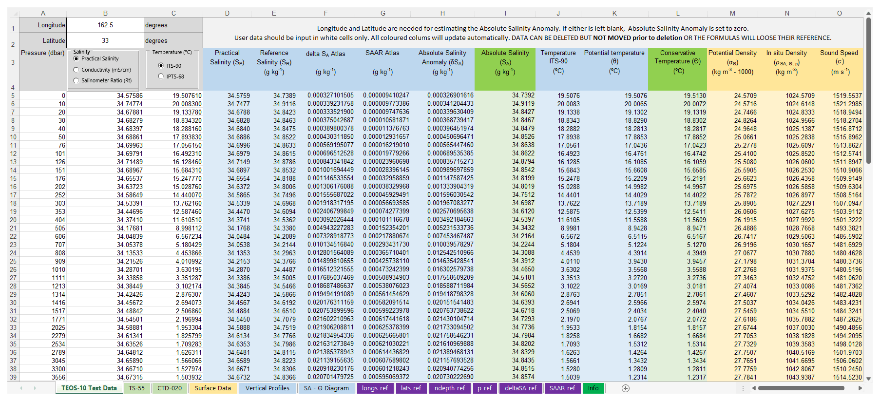
Figure 1 TEOS-10 Excel workbook (v.2.1) light green data tab. Seawater properties in coloured columns are computed on the fly from user data pasted into white cells.

2.1.1 Data input

• Location. The data template for the light green tabs was developed to process vertical casts located at a given location. Longitude and latitude must be input in cells “B1 : B2” in decimal format (degrees). Longitude can either be within the domain −180 to 180^∘ or 0 to 360^∘; i.e. 10^∘30^′ W can be input as −10.5 or 349.5^∘. The latitude domain is −90 to 90^∘; i.e. 30^∘ S would be −30^∘. The input of the cast coordinates is essential, as Absolute Salinity is dependent on location (Sect. 3.6). If either the longitude or the latitude cells are left empty, the salinity anomaly is set to zero and Absolute Salinity becomes equal to Reference Salinity.

• Pressure. Pressure (p) units are decibar. For seawater properties, pressure is always the pressure of the water column, i.e. absolute pressure subtracted by atmospheric pressure. Therefore, at the surface, p=0. For the upper ocean, 10 dbar ≈10 m.

• Salinity. The user can toggle the input between Practical Salinity (the salinity quantity which continues to be the recommended quantity to be archived (IOC, SCOR and IAPSO, 2010)), conductivity (mS cm⁻¹) (i.e. measured by an in situ transducer), or the salinometer ratio (Rt) (i.e. ratio between the conductivities of the sample and of Standard Seawater, measured by a laboratory salinometer). Column D of the spreadsheet (“Practical Salinity (S_P)”) either copies the S_P value if this was the salinity input or calculates S_P from conductivity using the function {SP_from_C(C,t,p)} or from the salinometer conductivity ratio using the function {SP_salinometer(Rt,t)}, depending on the radio button selected. In the latter option, t is the temperature of the thermostable bath of the laboratory salinometer.

• Temperature. Temperature (^∘C) may be selected to be either ITS-90 or IPTS-68 (data sets before 1990 are in the IPTS-68 standard, but recent data may still be applying this standard instead of the newer ITS-90 – checking the instrument specifications and/or the metadata associated with the data is advisable). Column J of the spreadsheet (“Temperature ITS-90”) either copies the temperature input if ITS-90 is selected or converts the IPTS-68 values to ITS-90 (ITS-90 = IPTS-68/1.00024). All functions use temperature ITS-90 as input.

2.2 The yellow Surface Data tab

The yellow Surface Data tab content differs from the other data spreadsheets on what refers to the input of the location coordinates. In this spreadsheet, longitude and latitude are input in the first two columns, allowing for the assignment of distinct coordinates for each line. This is useful if the data set is not a vertical cast at a given location but a set of measurements at different locations, typically at the same pressure level (e.g. surface measurements). Fictional data are included here to demonstrate the use of the template. The location of the first four data lines is in the Baltic Sea. Conditions in the Baltic are different from the open ocean (McDougall, 2010) and TEOS-10 treats this adjacent sea as being a specific case. Whilst for the world ocean the estimation of S_A depends on the measured salinity anomaly values at that location (look-up tables), for the Baltic Sea it is estimated by Eq. (1).

$$\begin{array}{}\text{(1)}& S_{\text{A}}\left(\text{Baltic}\right)=\left({\displaystyle \frac{\mathrm{35.16504}-\mathrm{0.087}}{\mathrm{35}}}\right)\times S_{\text{P}}+\mathrm{0.087}\end{array}$$

Whenever the location is in the Baltic (which is checked by the {is_Baltic(lon,lat)} function), the salinity anomaly cells display “Baltic”. This spreadsheet also includes a line with data from line 1 of the TEOS-10 Test Data tab (surface data from the NW Pacific) as well as a line of data without location coordinates (e.g. a sample from an estuary). In this case, salinity anomaly is set to zero and Absolute Salinity becomes equal to Reference Salinity.

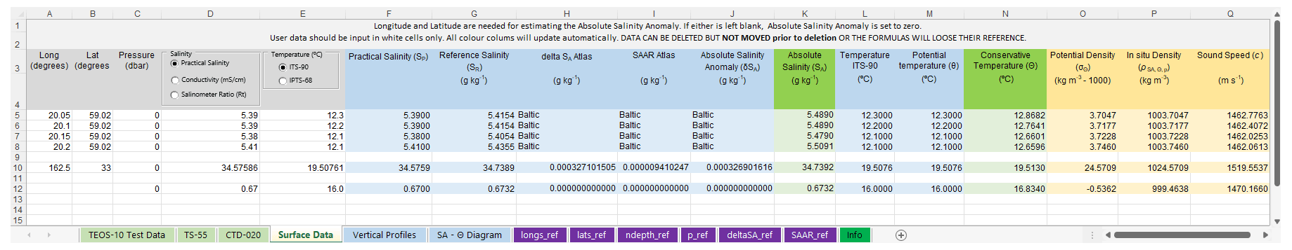
Figure 2 TEOS-10 Excel workbook (v.2.1) Surface Data tab. Surface data from different locations (location coordinates for each line). Four samples are from the Baltic Sea and one from the NW Pacific; the last sample (without long/lat coordinates) is from an estuary.

2.3 Vertical Profiles tab

The Vertical Profiles tab includes five plots that use the TS-55 and CTD-020 data sets and one plot with the TEOS-10 Test Data data set. Two of these plots are reproduced in Figs. 3 and 4. Changing the data will update the plots accordingly, and the user can add extra profiles by right-clicking the plot area, clicking “Select Data”, and then editing the data sources.

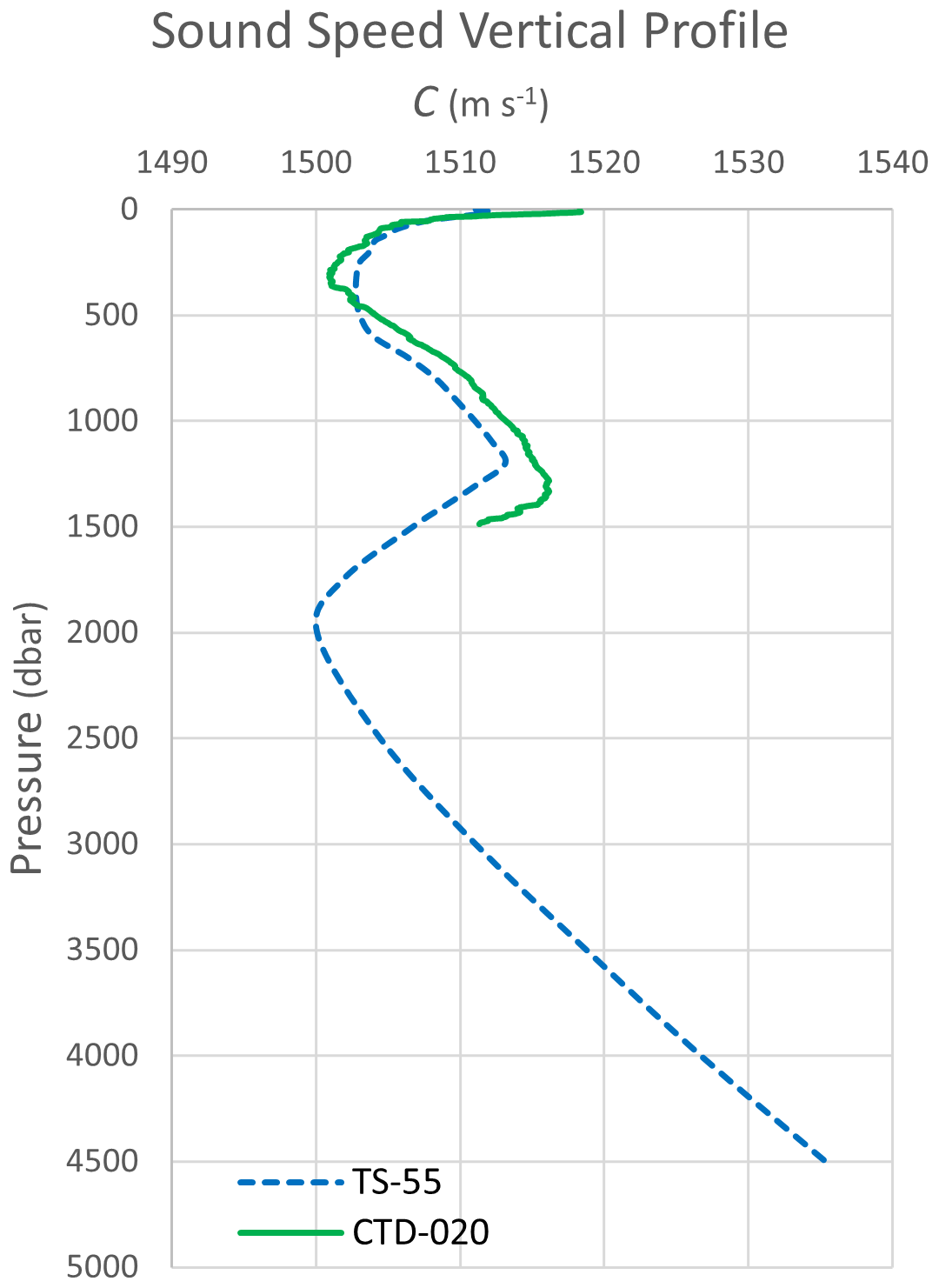
Figure 3 Sound speed vertical profile of two data sets included in TEOS-10 Excel. This plot is one of six included in the Vertical Profiles tab.

2.4 S_A–Θ Diagram tab

This is a template for plotting Absolute Salinity–Conservative Temperature diagrams. Since the introduction of TEOS-10, S_A–Θ diagrams have replaced T–S diagrams (EOS-80) for the characterisation of water masses in the ocean. The two diagrams represented (Fig. 5) are from the NW Pacific (TEOS-10 Test Data) and NE Atlantic (TS-55). Users can right-click the plot area, click “Select Data” and edit the data sources. The plot also shows the pressure values at selected points along the two S_A–Θ diagram lines (the label of the points is retrieved from the pressure data column in the respective data tab). These points can be individually selected and edited. The density field is shown through a set of σ_Θ dashed lines obtained from S_A–Θ pairs that resolve to constant values of σ_Θ (i.e. 24, 25, …, 29). As in all data spreadsheets, white cells can be edited. In this case, S_A extends from the x axis minimum (33.0) to the x axis maximum (38.0) with a 0.05 increment. The Conservative Temperature (Θ) values (green columns) are obtained by the function {sigma_CT_line(SA,sigma,min_temp, max_temp}. If more σ_Θ lines are desired, additional column pairs can be inserted into the spreadsheet and new series added to the plot.

2.5 The TEOS-10 look-up tabs (purple) a.k.a. the “Atlas”

Figure 6 shows the [ndepth_ref] look-up table which contains the number of pressure levels in each of the seawater samples that constitute the Atlas. On close inspection, it becomes apparent that the empty cells represent land, and the “white” shapes approximate to a map of the world land masses. The top of the spreadsheet is the South Pole, the bottom is the North Pole, and the Greenwich Meridian (0^∘ longitude) is to the left. Longitude is positive to the right, so actually the “map” is a skewed mirror image of the earth surface. Nonetheless, mirrored continental shapes are identifiable. The longitude bins (or cells) are referenced in the [longs_ref] look-up table, so the longitude of the cell highlighted in green in the upper left of Fig. 6, for which the x coordinate is 4 (fourth column), is 12^∘ E (value at the fourth line of the [longs_ref] table). This cell is at line 9 (y coordinate = 9) of the [ndepth_ref] table (Fig. 6), which, looking up in the [lats_ref] table, corresponds to −54^∘ of latitude. The green cell in Fig. 6 corresponds though to a reference cast located at 54^∘ S, 12^∘ E, with 41 pressure levels. These 41 pressure levels correspond to the pressure values indicated in the [p_ref] table. The [p_ref] table has level 22 (1010 dbar) highlighted in green, as this 3D location is used and referenced as a debug point in the {LookUp_atlas(table_name,p,lon,lat)} function, which retrieves data from the Absolute Salinity Anomaly [deltaSA_ref] and the Absolute Salinity Anomaly Ratio [SAAR_ref] look-up tables. The [ndepth_ref] table (Fig. 6) has 45 lines by 91 columns and so [deltaSA_ref] and [SAAR_ref], which both have the same size, have 4095 columns (45×91) by 45 lines (pressure levels). An additional numbering line (which does not affect how data are located) was added to facilitate debugging. Position (column number) in these tables is given by Eq. (2).

$$\begin{array}{}\text{(2)}& \text{Column}=\left(x-\mathrm{1}\right)\times \text{nlat}+y\end{array}$$

In Eq. (2), x is the longitude bin, y the latitude bin, and nlat the number of latitude bins (45). For the green cell, x=4 and y=9 as previously mentioned, so the anomaly data for this cell are located at column 144, line 22 (which corresponds to 1010 dbar) of the [deltaSA_ref] table. The Reference Salinity anomaly at 54^∘ S, 12^∘ E, and 1010 dbar is 0.008323162 g kg⁻¹ (also highlighted in green).

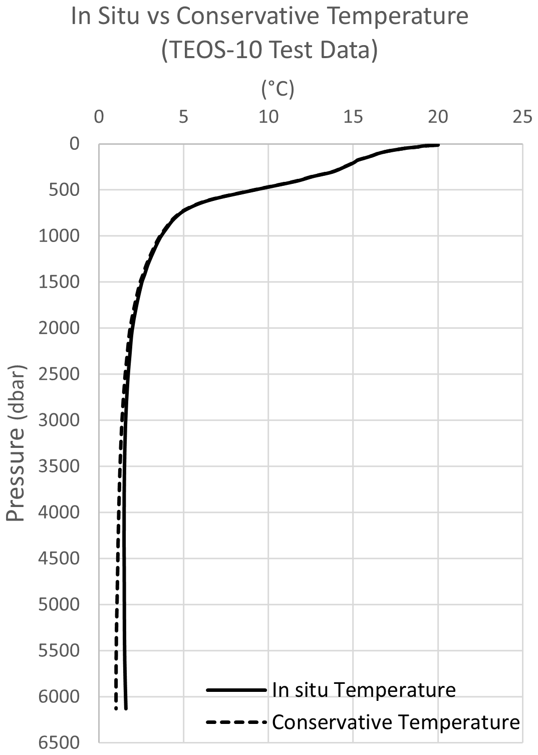
Figure 4 Comparison between in situ and Conservative Temperature of the TEOS-10 Test Data included in TEOS-10 Excel. This plot is one of six included in the Vertical Profiles tab.

2.6 Info tab (green)

This tab lists all released versions of TEOS-10 Excel, providing detailed information on the updates included in each version.

Table 1 List of all VBA modules and formulas included in TEOS-10 Excel (v.2.1). Direct translations from GSW are marked with “YES”, and original or modified functions are marked with “NO”.

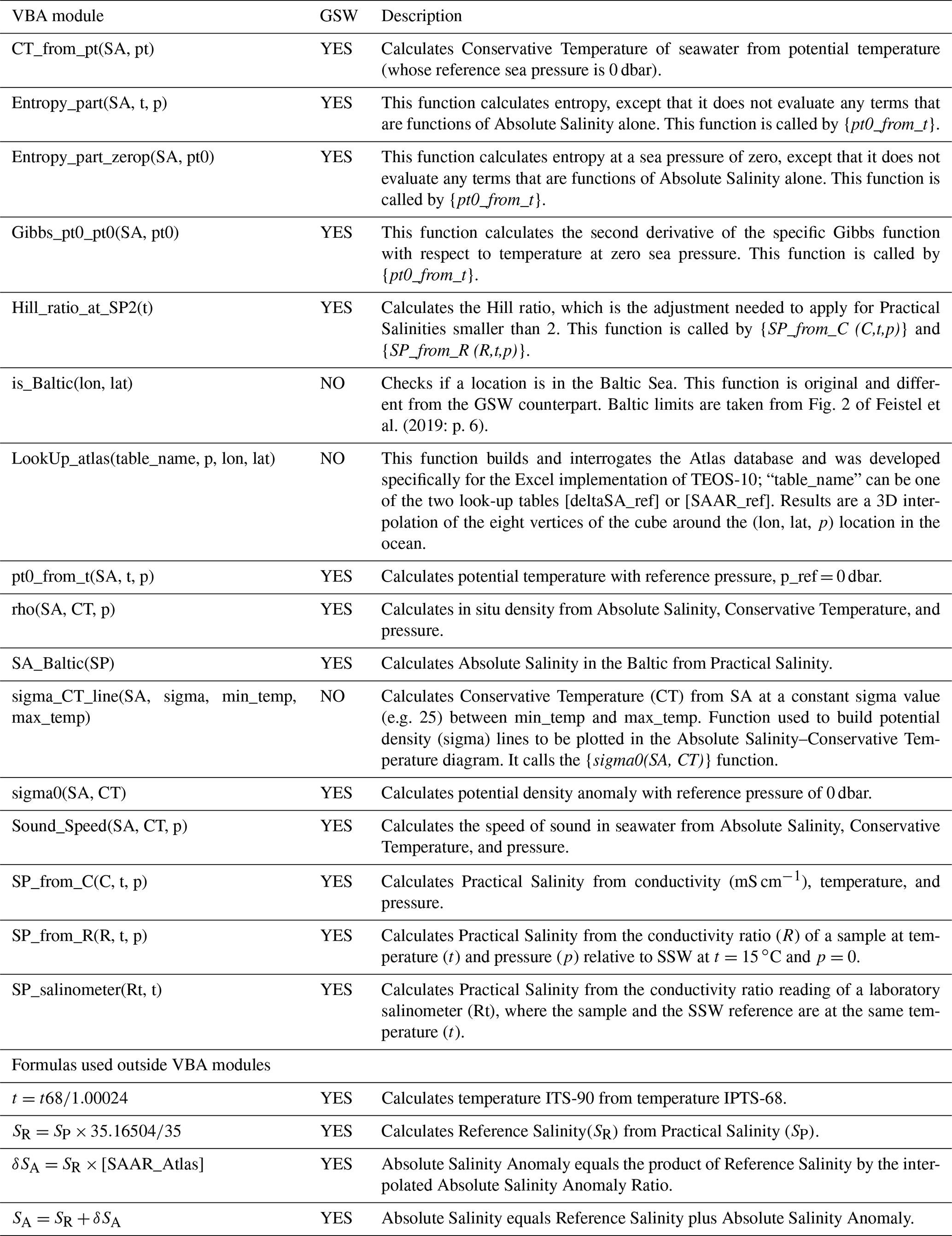
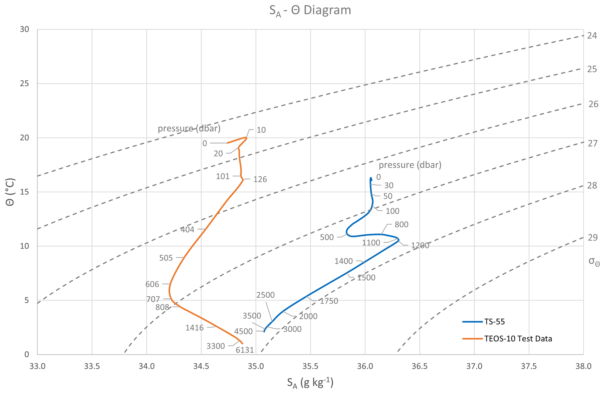
Figure 5 Absolute Salinity (S_A)–Conservative Temperature (Θ) diagrams. Data are from the TEOS-10 Test Data (NW Pacific) and TS-55 tab (NE Atlantic off the Iberian Peninsula). Pressure values are obtained dynamically from the data, and the density field (σ_Θ) is computed from data included in the spreadsheet template.

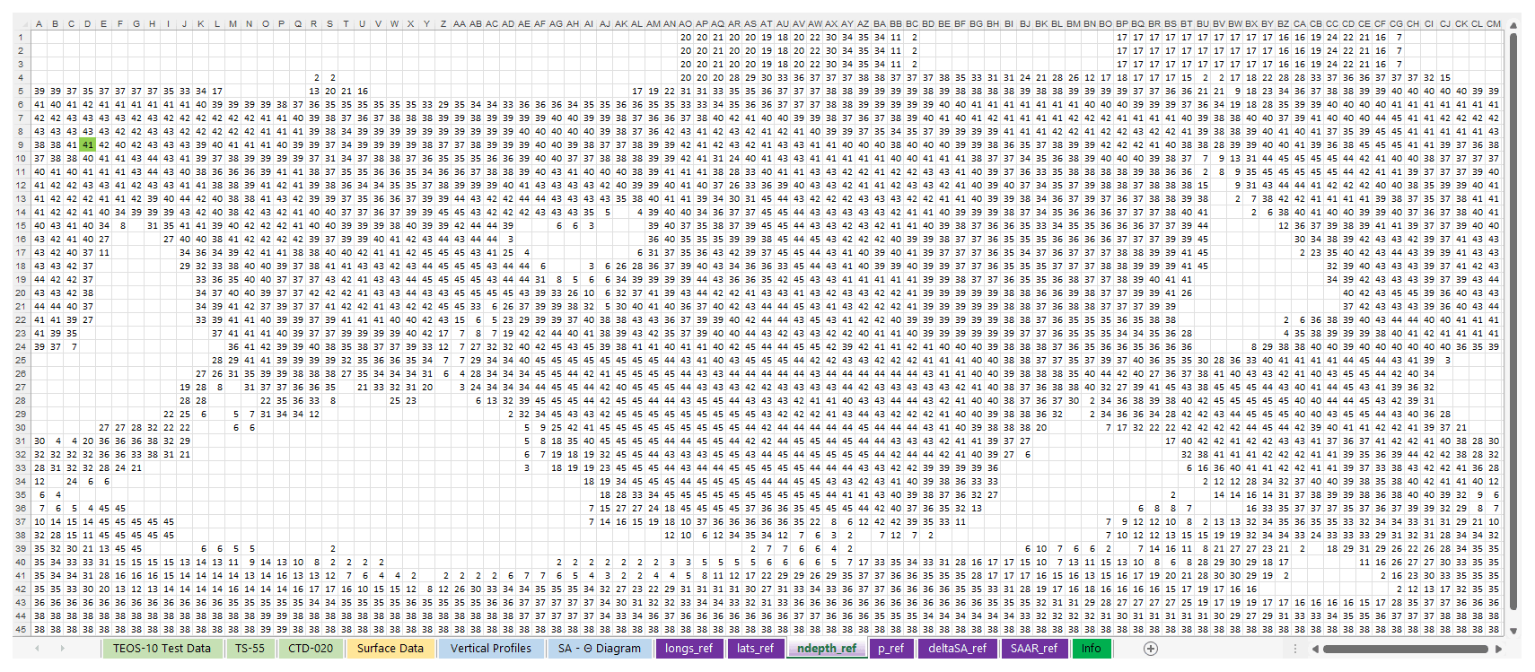
Figure 6 The [ndepth_ref] look-up table. The table has 45 rows (latitude) by 91 columns (longitude). South is at the top (first row is 86^∘ S) and first column is 0^∘ of longitude. The latitude × longitude grid is a $\mathrm{4}{}^{\circ }\times \mathrm{4}{}^{\circ }$ grid and each cell location is obtained from the [longs_ref] and [lats_ref] tables. Cell values are the number of pressure levels at the given location. The cell highlighted in green is used as a case study in the text.

3 VBA (Visual Basic for Applications) modules

Table 1 lists all functions (VBA modules) and formulas included in TEOS-10 Excel (v.2.1). Most modules are a direct translation into VBA of the GSW MATLAB counterpart (McDougall and Barker, 2011), and the original credit and references were kept in the code comments; however, due to the different way matrices are handled in MATLAB versus VBA, some functions needed to be redesigned, namely how accessing the Atlas look-up tables is managed. Returned values from TEOS-10 Excel are the same, for every parameter, as the ones obtained with the GSW toolbox up to 15 decimal places, i.e. difference = 0.000000000000000 (error checking was performed against MATLAB GSW toolbox version 3.06.12 from 25 May 2020). As referred to before, access to the VBA project environment can be obtained by pressing Alt + F11 (Windows) or Fn + Alt + F11 (Mac). All functions (alphabetically listed in Table 1) are described next, following the spreadsheet's column sequence.

3.1 Practical Salinity (S_P)

S_P is computed from conductivity using the function {SP_from_C(C,t,p)} or from the conductivity ratio (Rt) reading of a laboratory salinometer using the function {SP_salinometer(Rt,t)}, depending on the radio button selected. Practical Salinity is a dimensionless quantity, although PSU (Practical Salinity Unit) is commonly used. For reference, the calculation algorithm is designed so that the conductivity of Reference Composition Seawater at S_P=35, t₆₈=15, and p=0 is 42.9140 mS cm⁻¹, which can be used to validate the function. For the salinometer ratio function, a ratio = 1 will result in S_P=35, independently of the temperature. If S_P<2, both functions call the {Hill_ratio_at_SP2(t)} module which corrects the S_P value based on the Hill et al. (1986) algorithm. This algorithm is adjusted so that it is exactly equal to the Practical Salinity Scale−78 algorithm (Fofonoff and Millard, 1983) at S_P=2.

A VBA module to calculate Practical Salinity from the conductivity ratio (R), of a sample at temperature (t) and pressure (p) relative to SSW (Standard Seawater) at t=15 ^∘C and p=0 is also included as {SP_from_R(R,t,p)}, but it is not currently used in the template spreadsheets.

3.2 Reference Salinity (S_R)

Reference Salinity (S_R) is assumed to be proportional to Practical Salinity (IOC, SCOR and IAPSO, 2010) and obtained by Eq. (3). Units for S_R are grams per kilogram.

$$\begin{array}{}\text{(3)}& S_{\text{R}}={\displaystyle \frac{\mathrm{35.16504}}{\mathrm{35}}}\times S_{\text{P}}\end{array}$$

3.3 The delta S_A Atlas

The function {LookUP_atlas(table_name,p,lon,lat)} interrogates the Atlas database and was developed specifically for TEOS-10 Excel. The argument table_name can be one of the two look-up tables (“deltaSA_ref” or “SAAR_ref”) and the returned values are a 3D interpolation of the eight vertices of the cube around the location (Fig. 7). For the [deltaSA_ref] table, the result of the function is the Atlas Absolute Salinity Anomaly ($\mathit{\delta }{S}_{\text{A}}^{\text{atlas}})$. As the interpolation process is not clearly described in the GSW toolbox documentation, it is discussed next.

3.3.1 Interpolation

The function {LookUP_atlas(table_name,p,lon,lat)} begins by finding the grid point P1 of the 3D cube around the location (Fig. 7). P1 would be the grid point immediately before the latitude and longitude of a given location. The same applies to pressure. For example, if the spreadsheet data cell corresponds to a cast located at 1100 dbar, +13^∘ longitude, −51^∘ latitude, the grid position of P1(lon*, lat*, p^*) would be P1(4, 9, 22), obtained from the [longs_ref], [lats_ref], and [p_ref] tables. The other eight points are referenced to P1, by adding one unit to the grid position of P1 as shown in Fig. 1.

Figure 7 3D interpolation cube. Points are defined by their grid position (lon*, lat*, p^*).

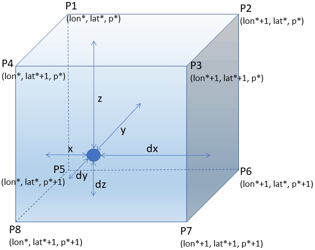
The standard basic 3D interpolation model assumes that the cube dimensions are $\mathrm{1}\times \mathrm{1}\times \mathrm{1}$ (Bourke, 1999), and the distances dx, dy and dz are obtained by subtracting, respectively, x, y, and z from the unit; however, in this case, the longitude and latitude grid space are 4^∘ and the pressure difference between the upper and bottom points varies from grid level to grid level (e.g. 10 dbar between levels 1 and 2 but 101 dbar between levels 22 and 23). Distances x, y, and z are obtained from Eqs. (4, 5, and 6), and then dx, dy, and dz from Eq. (7).

$$\begin{array}{}\text{(4)}& {\displaystyle }x=\left(\text{long}-\text{long(P1)}\right)/\mathrm{4}\text{(5)}& {\displaystyle }y=\left(\text{lat}-\text{lat(P1)}\right)/\mathrm{4}\text{(6)}& {\displaystyle }z=\left(p-p\left(\text{P1}\right)\right)/\left(p\left(\text{P5}\right)-p(\text{P1}\right))\text{(7)}& {\displaystyle }\mathrm{d}x=\mathrm{1}-x,\mathrm{d}y=\mathrm{1}-y,\mathrm{d}z=\mathrm{1}-z\end{array}$$

The interpolated value (v) is obtained by weighing the contribution of the eight points according to Eqs. (8 to 16), where v(Pn) is the $\mathit{\delta }{S}_{\text{A}}^{\text{atlas}}$ value at Pn (from [deltaSA_table]).

$$\begin{array}{}\text{(8)}& {\displaystyle }v\mathrm{1}=v\left(\text{P1}\right)\times \mathrm{d}x\times \mathrm{d}y\times \mathrm{d}z\text{(9)}& {\displaystyle }v\mathrm{2}=v\left(\text{P2}\right)\times x\times \mathrm{d}y\times \mathrm{d}z\text{(10)}& {\displaystyle }v\mathrm{3}=v\left(\text{P3}\right)\times x\times y\times \mathrm{d}z\text{(11)}& {\displaystyle }v\mathrm{4}=v\left(\text{P4}\right)\times \mathrm{d}x\times y\times \mathrm{d}z\text{(12)}& {\displaystyle }v\mathrm{5}=v\left(\text{P5}\right)\times \mathrm{d}x\times \mathrm{d}y\times z\text{(13)}& {\displaystyle }v\mathrm{6}=v\left(\text{P6}\right)\times x\times \mathrm{d}y\times z\text{(14)}& {\displaystyle }v\mathrm{7}=v\left(\text{P7}\right)\times x\times y\times z\text{(15)}& {\displaystyle }v\mathrm{8}=v\left(\text{P8}\right)\times \mathrm{d}x\times y\times z\text{(16)}& {\displaystyle }v=v\mathrm{1}+v\mathrm{2}+v\mathrm{3}+v\mathrm{4}+v\mathrm{5}+v\mathrm{6}+v\mathrm{7}+v\mathrm{8}\end{array}$$

3.3.2 Missing data

There are pressure levels in the Atlas reference casts where data are missing. Figure 8 illustrates this situation.

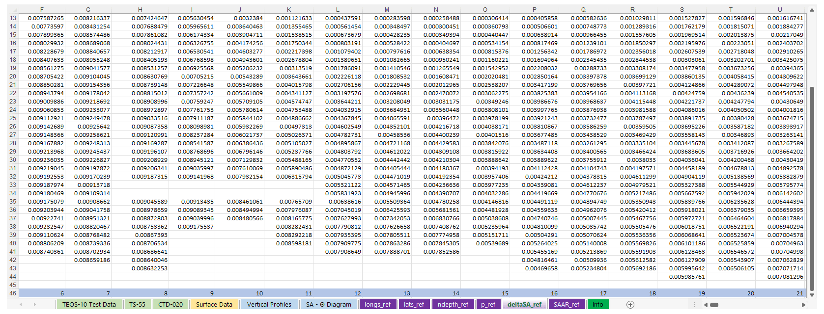
Figure 8 The [deltaSA_ref] table: reference data missing for pressure levels 33 and 34 of columns 8, 9, 10, and 11.

The GSW toolbox fills these gaps by averaging the neighbouring four points in the grid at the same pressure level. As the ocean is horizontally stratified, this is logical, but neighbour points themselves might also lack data at the same level, which may compromise the result. A $\mathit{\delta }{S}_{\text{A}}^{\text{atlas}}$ plot from [deltaSA_ref] column 8 (0^∘ long, −54^∘ lat) is shown in Fig. 9. The $\mathit{\delta }{S}_{\text{A}}^{\text{atlas}}$ output of the GSW toolbox and TEOS-10 Excel is the same for the part where there are data (blue line), but the output of the GSW toolbox for the two pressure levels where data are missing is clearly off the profile (orange). In this situation, TEOS-10 Excel implements a vertical interpolation within the vertical profile, which resolves the missing data situations better (green in Fig. 9). The second case where the GSW toolbox seems to be less consistent is when not all points of the 3D interpolation cube exist at the last pressure level. The GSW toolbox test data (included in the TEOS-10 Test Data tab) are such an example (Fig. 10). The GSW toolbox approach for resolving missing data on the last pressure level is as before. In these situations, if one of the four bottom points of the interpolation cube (P5, P6, P7, or P8 in Fig. 7) is missing, TEOS-10 Excel assigns to it the same value as the next upper point at that location (e.g. v(P7) = v(P3)). The subsequent resulting profile is potentially more consistent in TEOS-10 Excel than would be available in the GSW toolbox (Fig. 10).

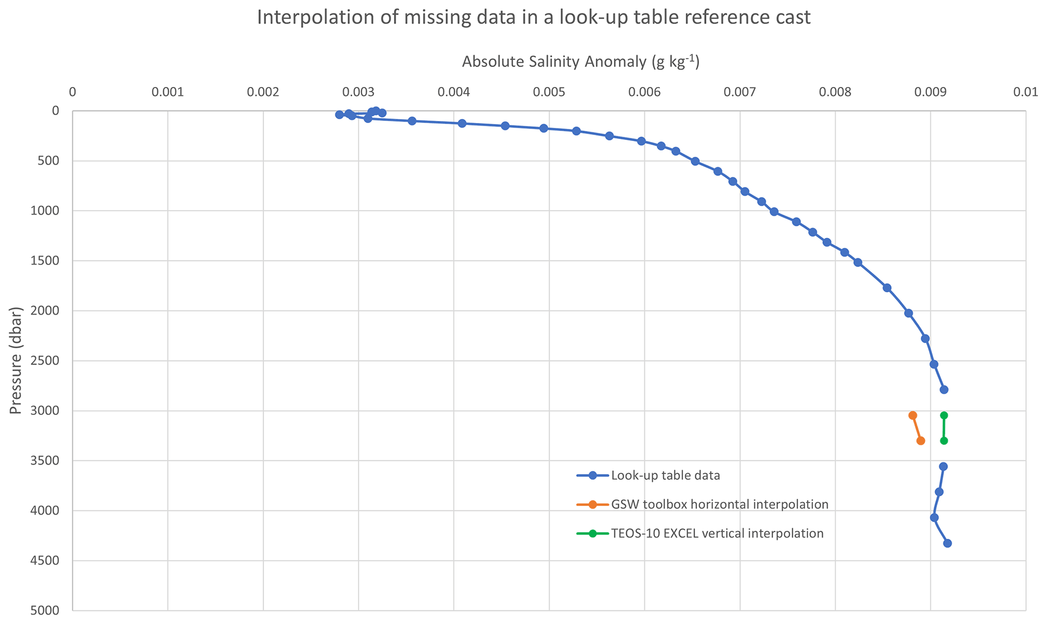
Figure 9 The $\mathit{\delta }{S}_{\text{A}}^{\text{atlas}}$ plot from [deltaSA_ref], column 8. Missing data at levels 33 and 34 (3045 and 3300 dbar) are not well resolved by horizontal interpolation (GSW toolbox). Vertical interpolation implemented in TEOS-10 Excel resolves these situations better.

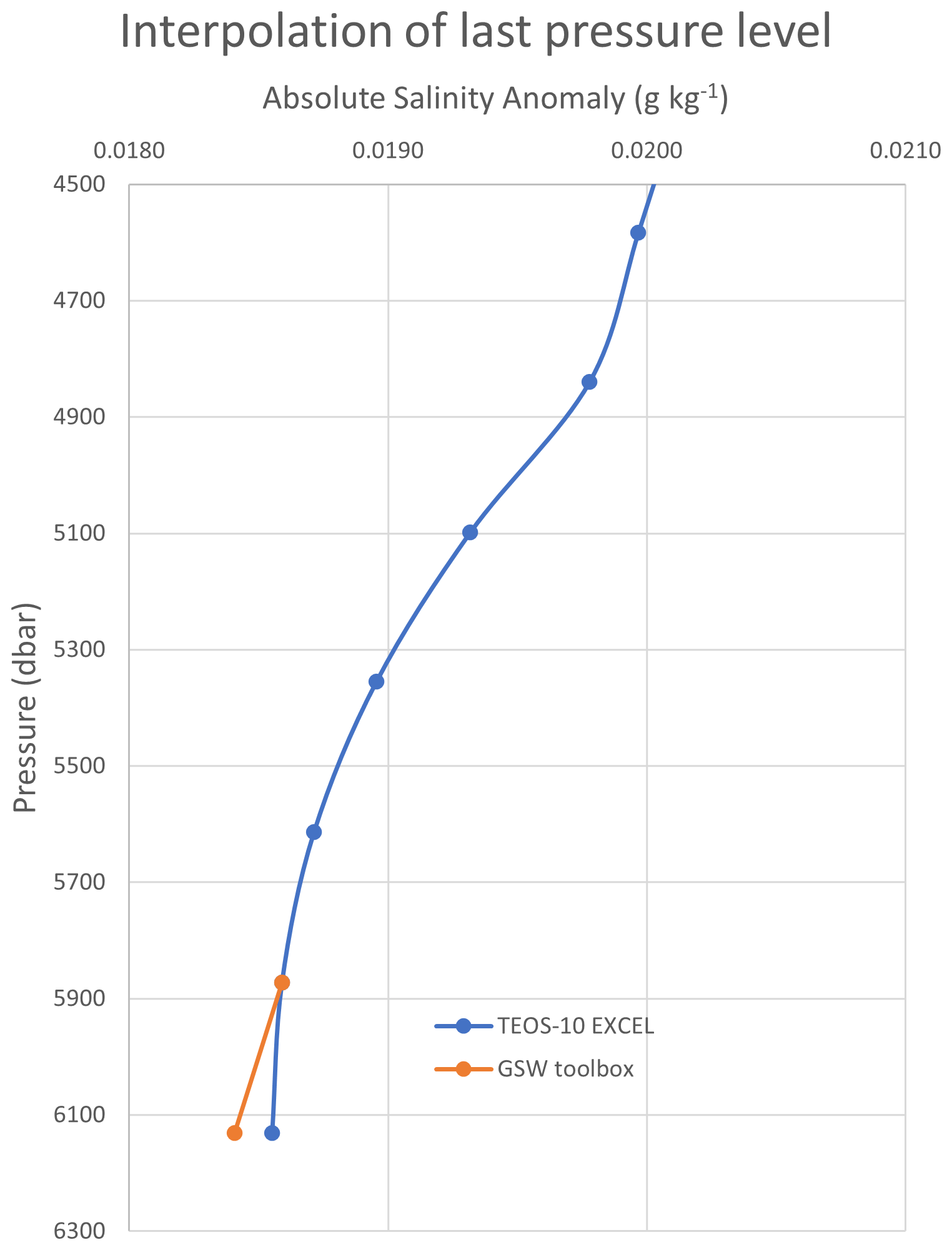
Figure 10 The $\mathit{\delta }{S}_{\text{A}}^{\text{atlas}}$ plot from the TEOS-10 Test Data tab. Not all neighbour points have data at the last pressure level. For these points, TEOS-10 Excel uses the same value as of their last pressure level to resolve the 3D interpolation cube, while the GSW toolbox averages the same level data from neighbouring points.

3.4 delta SAAR Atlas

The Atlas Absolute Salinity Anomaly Ratio (R^δ) is obtained by the function {LookUP_atlas(table_name,p,lon,lat)}, exactly as for the Absolute Salinity Anomaly (Sect. 3.3) but calling it with SAAR_ref as the table_name argument. R^δ is the quantity used to estimate the Absolute Salinity Anomaly (Sect. 3.5), which is then used for obtaining Absolute Salinity (Sect. 3.6).

3.5 Absolute Salinity Anomaly

The Absolute Salinity Anomaly (δS_A) is the product of the Atlas Absolute Salinity Anomaly Ratio and Reference Salinity (Eq. 17).

$$\begin{array}{}\text{(17)}& \mathit{\delta }{S}_{\text{A}}=R^{\mathit{\delta }}\times S_{\text{R}}\end{array}$$

3.6 Absolute Salinity

Absolute Salinity (S_A) is the sum of Reference Salinity and salinity anomaly (Eq. 18).

$$\begin{array}{}\text{(18)}& S_{\text{A}}=S_{\text{R}}+\mathit{\delta }{S}_{\text{A}}\left(\mathrm{g}{\mathrm{kg}}^{-\mathrm{1}}\right)\end{array}$$

If the location is in the Baltic Sea, the world atlas salinity anomalies do not apply (McDougall, 2010) and Absolute Salinity is computed algebraically from Practical Salinity with the function {SA_Baltic(SP)}, which applies Eq. (19).

$$\begin{array}{}\text{(19)}& S_{\text{A}}^{\text{Baltic}}={\displaystyle \frac{\left(\mathrm{35.16504}-\mathrm{0.087}\right)}{\mathrm{35}}}\times S_{\text{P}}+\mathrm{0.087}\left(\mathrm{g}{\mathrm{kg}}^{-\mathrm{1}}\right)\end{array}$$

Limits for the Baltic were taken from Fig. 2 of Feistel et al. (2010). The function {is_Baltic(lon,lat)} checks if the location is in the Baltic Sea by finding out if the coordinates lie within either of two rectangular areas defined by [52^∘ N: 60^∘ N, 9^∘ E: 15^∘ E] and [52^∘ N: 67^∘ N, 15^∘ E: 30^∘ E].

3.7 Temperature ITS-90

The temperature standard used in TEOS-10 as argument to all functions is ITS-90 (Preston-Thomas, 1990). If the ITS-90 radio button is selected (column C of the spreadsheet), the temperature input values are copied; if IPTS-68 is selected instead, the IPTS-68 temperature will be converted to ITS-90 using Eq. (20).

$$\begin{array}{}\text{(20)}& t_{\mathrm{ITS}-\mathrm{90}}=t_{\mathrm{IPTS}-\mathrm{68}}/\mathrm{1.00024}\left({}^{\circ }C\right)\end{array}$$

3.8 Potential temperature (θ)

Potential temperature (θ, ^∘C) is obtained by the function {pt0_from_t(SA,t,p)}. Three other functions – {Entropy_part(SA,t,p)}, {Entropy_part_zerop(SA,pt0)}, and {Gibbs_pt0_pt0(SA,pt0)} – are called within the computation process. These four functions are a VBA translation of the original GSW toolbox counterparts (IOC, SCOR and IAPSO, 2010; McDougall and Wotherspoon, 2013).

3.9 Conservative Temperature (Θ)

Conservative Temperature (Θ, ^∘C) is the temperature quantity used as argument in the Thermodynamic Equation Of Seawater – 2010 (IOC, SCOR and IAPSO, 2010). It is obtained with the function {CT_from_pt(SA,pt)}, which is a direct translation from the GSW toolbox counterpart and estimates Θ from S_A and θ.

3.10 Potential density (σ_Θ)

Potential density (σ_Θ, kg m${}^{-\mathrm{3}}-\mathrm{1000}$) with reference to a sea pressure of 0 dbar is estimated by the function {sigma0(SA,CT)}, the arguments of which are Absolute Salinity (S_A) and Conservative Temperature (Θ). This function uses the TEOS-10 75-term equation and is a VBA translation of the original GSW toolbox counterpart (IOC, SCOR and IAPSO, 2010; McDougall et al., 2003; Roquet et al., 2015).

3.11 In situ density (${\mathit{\rho }}_{S_{\mathrm{A}},\mathrm{\Theta },p}$)

In situ density (${\mathit{\rho }}_{S_{\mathrm{A}},\mathrm{\Theta },p}$, kg m⁻³) is estimated by the function {rho(SA,CT,p)}, whose arguments are Absolute Salinity (S_A), Conservative Temperature (Θ), and pressure (p). This function uses the TEOS-10 75-term equation and is a VBA translation of the original GSW toolbox counterpart (IOC, SCOR and IAPSO, 2010; McDougall et al., 2003; Roquet et al., 2015).

3.12 Sound speed (c)

Sound speed (c, m s⁻¹) is estimated by the function {Sound_Speed(SA,CT,p)}, whose arguments are Absolute Salinity (S_A), Conservative Temperature (Θ), and pressure (p). This function uses the TEOS-10 75-term equation and is a VBA translation of the original GSW toolbox counterpart (IOC, SCOR and IAPSO, 2010; McDougall et al., 2003; Roquet et al., 2015).

3.13 The [deltaSA_ref] table not required

The Atlas Absolute Salinity Anomaly (column F of the data spreadsheets) is not used for any calculation, as Absolute Salinity Anomaly (δS_A) is obtained from the product of the Absolute Salinity Anomaly Ratio (R^δ) and Reference Salinity (Eq. 17), and R^δ is retrieved from the [SAAR_ref] look-up table. However, the [deltaSA_ref] look-up table is not necessary for any computation and can eventually be deleted from the Excel workbook for brevity; however, this table was used as a debugging tool in the development of the VBA functions, and the error checking and interpolation improvements described in Sect. 3.3 refer to this look-up table, which is why it was included in TEOS-10 Excel as a supporting element for this paper. Additionally, users might be interested in ascertaining the Absolute Salinity Anomaly for a given location or perform further error checking, comparing TEOS-10 Excel output against the GSW toolbox for other data sets.

4 Conclusions

To our knowledge, TEOS-10 Excel is the first implementation of the Thermodynamic Equation Of Seawater – 2010 outside the official GSW toolboxes. It does not aim to reproduce the full-featured GSW environment as it implements only a small subset of the TEOS-10 functions. Opening the possibility of estimating a relevant set of seawater parameters within a well-known and friendly environment (Excel), however, will hopefully democratise the compliance with current oceanographic standards among a large community of researchers and students who are not at ease with the use of high-level programming languages. As discussed in the paper, some issues were detected with the GSW interpolation when there are missing data in the Atlas reference tables. In these cases, TEOS-10 Excel adopts an alternative approach to the interpolation method, which has produced better results (Sect. 3.3.2). Nonetheless, this is perhaps a situation that deserves further research.