Arctic sea level variability from high-resolution model simulations and implications for the Arctic observing system

Two high-resolution model simulations are used to investigate the spatiotemporal variability of the Arctic Ocean sea level. The model simulations reveal barotropic sea level variability at periods of < 30 d, which is strongly captured by bottom pressure observations. The seasonal sea level variability is driven by volume exchanges with the Pacific and Atlantic oceans and the redistribution of the water by the wind. Halosteric effects due to river runoff and evaporation minus precipitation ice melting/formation also contribute in the marginal seas and seasonal sea ice extent regions. In the central Arctic Ocean, especially the Canadian Basin, the decadal halosteric effect dominates sea level variability. The study confirms that satellite altimetric observations and Gravity Recovery and Climate Experiment (GRACE) could infer the total freshwater content changes in the Canadian Basin at periods longer than 1 year, but they are unable to depict the seasonal and subseasonal freshwater content changes. The increasing number of profiles seems to capture freshwater content changes since 2007, encouraging further data synthesis work with a more complicated interpolation method. Further, in situ hydrographic observations should be enhanced to reveal the freshwater budget and close the gaps between satellite altimetry and GRACE, especially in the marginal seas.

1 Introduction

The Arctic Ocean is experiencing pronounced changes (e.g., Perovich et al., 2020; AMAP, 2019). Observations have revealed increased warm inflows through the Bering Strait (Woodgate et al., 2012) and the Fram Strait (Polyakov et al., 2017), and an unprecedented freshening of the Canadian Basin, especially the Beaufort Gyre (Proshutinsky et al., 2019). The rapid changes potentially impact the weather and climate of the Northern Hemisphere (Overland et al., 2021).

As an integrated indicator, sea level change reflects changing ocean conditions caused by ocean dynamics, atmospheric forcing, and terrestrial processes (Stammer et al., 2013). Satellite altimetry, together with bottom pressure observations from Gravity Recovery and Climate Experiment (GRACE), has been applied to infer ocean temperature and salinity changes that are not measured directly in the Arctic Ocean (e.g., Armitage et al., 2016) and in the deep ocean (e.g., Llovel et al., 2014), enhancing our ability to monitor ocean changes.

Over the past decades, coupled ocean–sea ice models and observations have advanced our understanding of the Arctic Ocean variability. Proshutinsky and Johnson (1997) demonstrated wind-forced cyclonic/anticyclonic ocean circulation patterns accompanied by dome-shaped sea levels variation using a barotropic model simulation. Further, ocean circulation changes in the Canadian Basin result in freshwater accumulation and release, which is very well correlated to sea level changes (Koldunov et al., 2014; Proshutinsky et al., 2002). Given that sea level changes reflect freshwater content changes in the Canadian Basin, Giles et al. (2012) and Morison et al. (2012) proposed to use satellite altimetry observations and GRACE observations to infer freshwater content changes. The method was then applied to explore the freshwater content changes in the Beaufort Gyre (Armitage et al., 2016; Proshutinsky et al., 2019) at seasonal to decadal timescales. In the Barents Sea, Volkov et al. (2013) used altimetric sea level observations and the ECCO reanalysis (Forget et al., 2015) to explore seasonal to interannual sea level anomalies (SLAs), revealing different roles of mass-related changes, thermosteric and halosteric effects on different regions of the Barents Sea.

However, the sparseness of in situ profiles, coarse resolution and significant uncertainties of satellite altimetry and GRACE observations result in large gaps in understanding the spatiotemporal variability of the Arctic sea level and its relations to the thermo-/halosteric effects and mass changes (Ludwigsen and Andersen, 2021). Previous studies mainly focus on the decadal sea level variability (e.g., Koldunov et al., 2014; Proshutinsky et al., 2007; Proshutinsky and Johnson, 1997), and no study has yet fully explored the Arctic sea level variability at different spectral bands, and its dependence on the mass component and the vertical oceanic variability. Such a study could help identify critical regions and environmental parameters that need to be observed coordinately and point out observational gaps that need to be filled in the future.

Our study systematically explores the Arctic sea level variability as a function of timescale and geographic location using daily and monthly outputs of two high-resolution model simulations. Contributions from barotropic changes expressed in bottom pressure variations and baroclinic processes represented by thermo-/halosteric changes are quantified at different timescales. Altimetric and GRACE measurements, in situ hydrographic observations mapped with different interpolation schemes (e.g., Haine et al., 2015; Polyakov et al., 2008; Rabe et al., 2011, 2014), and ocean reanalyses have been used to infer the basin-scale freshwater changes during the unprecedented freshwater changes since the 2000s. However, Solomon et al. (2021) pointed out that significant uncertainties and discrepancies remain in revealing the regional patterns. This study further discusses the existing Arctic observing system's capability to monitor the Arctic freshwater content variability and identify observational gaps.

The structure of the remaining paper is as follows: the numerical models and the observations from the bottom pressure sensor, GRACE, and satellite altimetry are described in Sect. 2, together with different components of sea level changes. We compare the model simulations against observations in Sect. 3. Section 4 analyzes sea level variability and associated mechanisms at high frequency (<30 d), seasonal cycles, and decadal timescales. The relations with bottom pressure and thermo-/halosteric components are demonstrated, pointing out key regions and parameters we need to observe. Further, we analyze the ability of satellite altimetry, GRACE, and the in situ profiler system to monitor the Arctic freshwater content variability in Sect. 5. Section 6 provides a summary and conclusions.

2 Model simulations and observations

2.1 Atlantic–Arctic simulations

This study relies on two ocean high-resolution numerical simulations using the Massachusetts Institute of Technology general circulation model (MITgcm, Marshall et al., 1997). A dynamic–thermodynamic sea ice model (Hibler, 1979, 1980; Zhang and Rothrock, 2000), implemented by Losch et al. (2010), is employed to simulate sea ice processes. The model domain covers the entire Arctic Ocean north of the Bering Strait and the Atlantic Ocean north of 33^∘ S. In the horizontal, the model uses a curvilinear grid with resolutions of ∼8 km (ATLARC08km) and ∼4 km (ATLARC04km). In the vertical, ATLARC08km has 50 levels with resolution ranging from 10 m over the top 130 to 456.5 m in the deep basin. And ATLARC04km has 100 z levels ranging from 5 m over the top 200 to 185 m in the deep basin.

At the ocean surface, the model simulations are forced by momentum, heat, and freshwater fluxes computed using bulk formulae and either the 6-hourly NCEP RA1 reanalysis (Kalnay et al., 1996) (ATLARC08km) or the 6-hourly ECMWF ERA-Interim reanalysis (Dee et al., 2011) (ATLARC04km). A virtual salt flux parameterization is used to mimic the dilution and salinification effects of rainfall, evaporation, and river discharge. The models are forced by the monthly output from the GECCO2 (Köhl, 2015) global model configuration at the open boundaries. The river runoff is applied at river mouths by seasonal climatology (Fekete et al., 2002). Bottom topography is derived from the ETOPO 2 min (Smith and Sandwell, 1997) database. ATLARC08km is initialized with annual mean temperature and salinity from the World Ocean Atlas 2005 (Boyer et al., 2005) and covers 1948 to 2016, and ATLARC04km starts from the initial condition, including velocity, temperature, and salinity, of ATLARC08km at the start of the year 2002. Table 1 summarizes both the simulations and their main characteristics.

Table 1 Summary of model simulations used in this study.

2.2 Satellite and in situ observations

Koldunov et al. (2014) have validated ATLARC08km against tide gauge observations. We further compare the two model simulations against in situ bottom pressure observations, GRACE observations, and satellite altimetric observations.

The monthly altimetric sea level observations from Armitage et al. (2016, http://www.cpom.ucl.ac.uk/dynamic_topography/, last access: 4 January 2022) and GRACE measurements (Chambers and Bonin, 2012, https://doi.org/10.5067/TEOCN-3AJ64) are used in comparison with the model simulations. For the very high-frequency variability, bottom pressure records supplied by the Beaufort Gyre Exploration Project (BGEP, M_a, M_b, M_c, and M_d in Fig. 1, https://www2.whoi.edu/site/beaufortgyre/data/mooring-data/, last access: 4 January 2022) and the North Pole Environmental Observatory (NPEO, M_npeo in Fig. 1, ftp://northpoleftp.apl.washington.edu/NPEO_Data_Archive/, last access: 11 November 2021) are used. Tidal signals are removed using the T_TIDE MATLAB program (Pawlowicz et al., 2002) since the model did not include tidal forcing.

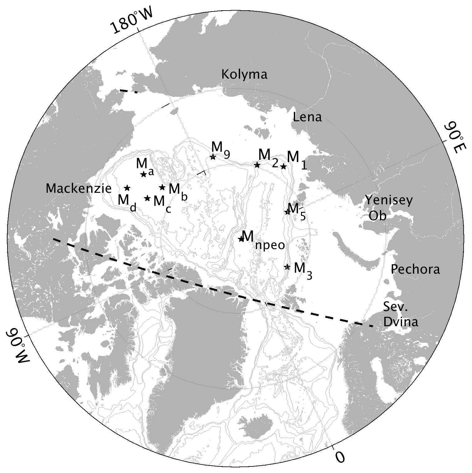
Figure 1 A map of the pan-Arctic Ocean presenting the locations of moorings deployed by the Nansen and Amundsen Basin Observational System (NABOS, black stars labeled M₁, M₂, M₃, M₅, and M₉), by the Beaufort Gyre Exploration Project (BGEP, black stars marked as M_a, M_b, M_c, M_d), and by the North Pole Environmental Observatory (NPEO, black star labeled M_npeo). The dashed black lines enclose the Arctic regions used in the following sections. Bathymetry contours of 500, 1000, 2000, 3000, and 4000 m are drawn with gray lines. Main rivers are labeled with their names near the river mouths.

2.3 Relation between sea level, bottom pressure, and thermo-/halosteric components

Following Ponte (1999) and Calafat et al. (2013), sea level anomaly η^′, can be separated into a steric component ${\mathit{\eta }}_{\mathrm{s}}^{\prime }$ due to density change, an inverse barometer effect ${\mathit{\eta }}_{\mathrm{IB}}^{\prime }$, and a mass (measured by bottom pressure observations) component ${\mathit{\eta }}_{\mathrm{m}}^{\prime }$:

$$\begin{array}{}\text{(1)}& {\mathit{\eta }}^{\prime }=-{\displaystyle \frac{\mathrm{1}}{{\mathit{\rho }}_{\mathrm{0}}}}\underset{-H}{\overset{\mathrm{0}}{\int }}{\mathit{\rho }}^{\prime }\mathrm{d}z+{\displaystyle \frac{\mathrm{1}}{{\mathit{\rho }}_{\mathrm{0}}g}}\left(\stackrel{\mathrm{‾}}{P_{\mathrm{a}}^{\prime }}-P_{\mathrm{a}}^{\prime }\right)+{\displaystyle \frac{\mathrm{1}}{{\mathit{\rho }}_{\mathrm{0}}g}}\left(P_{\mathrm{b}}^{\prime }-\stackrel{\mathrm{‾}}{P_{\mathrm{a}}^{\prime }}\right),\end{array}$$

where g=9.8 m s⁻² is the gravitational acceleration. The first term on the right-hand side represents the steric effect ${\mathit{\eta }}_{\mathrm{s}}^{\prime }$, with ρ₀ being a reference density (1025.0 kg m⁻³ in this study) and ρ^′ being the density change. The second term is the inverse barometer effect ${\mathit{\eta }}_{\mathrm{IB}}^{\prime }$: $\stackrel{\mathrm{‾}}{P_{\mathrm{a}}^{\prime }}$ and $P_{\mathrm{a}}^{\prime }$ represent air pressure anomalies average over the global ocean and at the observing location, respectively. The last term defines the mass component ${\mathit{\eta }}_{\mathrm{m}}^{\prime }$. $P_{\mathrm{b}}^{\prime }$ is the bottom pressure anomalies in equivalent meters of water.

Since the model simulations do not include the impacts of surface air pressure anomalies, the model-simulated sea level changes due to steric and mass components are simplified as

$$\begin{array}{}\text{(2)}& {\mathit{\eta }}^{\prime }=-{\displaystyle \frac{\mathrm{1}}{{\mathit{\rho }}_{\mathrm{0}}}}\underset{-H}{\overset{\mathrm{0}}{\int }}{\mathit{\rho }}^{\prime }\mathrm{d}z+{\displaystyle \frac{\mathrm{1}}{{\mathit{\rho }}_{\mathrm{0}}g}}\left(P_{\mathrm{b}}^{\prime }\right).\end{array}$$

Separating density changes into temperature and salinity changes, we decompose the steric height ${\mathit{\eta }}_{\mathrm{s}}^{\prime }$ into thermosteric height ${\mathit{\eta }}_{\mathrm{st}}^{\prime }$ (due to temperature anomalies) and halosteric height ${\mathit{\eta }}_{\mathrm{ss}}^{\prime }$ (due to salinity anomalies):

$$\begin{array}{}\text{(3)}& {\displaystyle }& {\displaystyle }{\mathit{\eta }}_{\mathrm{st}}^{\prime }=-{\displaystyle \frac{\mathrm{1}}{{\mathit{\rho }}_{\mathrm{0}}}}\underset{-H}{\overset{\mathrm{0}}{\int }}\left(\mathit{\rho }\right(T,\stackrel{\mathrm{‾}}{S},p)-\mathit{\rho }(\stackrel{\mathrm{‾}}{T},\stackrel{\mathrm{‾}}{S},p\left)\right)\mathrm{d}z,\text{(4)}& {\displaystyle }& {\displaystyle }{\mathit{\eta }}_{\mathrm{ss}}^{\prime }=-{\displaystyle \frac{\mathrm{1}}{{\mathit{\rho }}_{\mathrm{0}}}}\underset{-H}{\overset{\mathrm{0}}{\int }}\left(\mathit{\rho }\right(\stackrel{\mathrm{‾}}{T},S,p)-\mathit{\rho }(\stackrel{\mathrm{‾}}{T},\stackrel{\mathrm{‾}}{S},p\left)\right)\mathrm{d}z,\end{array}$$

where T, S, and p represent seawater temperature, salinity, and pressure. The overbars denote the average over the simulation time.

Before comparing the model simulation with the GRACE measurements and mooring-based bottom pressure observations, we remove air pressure anomalies averaged over the global ocean $\stackrel{\mathrm{‾}}{P_{\mathrm{a}}^{\prime }}$, and then global-mean mass changes from GRACE-based bottom pressure observations since the virtual salt flux parameterization does not include mass transfer from land to ocean. In total, this process removes a seasonal cycle with an amplitude of ∼1–1.5 cm from the measurements.

3 Testing simulations against observations

Koldunov et al. (2014) have demonstrated that the interannual sea level variability in ATLARC08km and tide gauges match very well. In the present study, we further evaluate the skill of the model-simulated sea level and bottom pressure variability by comparing the root mean square (rms) variability of sea level and bottom pressure against altimetric data (Armitage et al., 2016) and GRACE data (Chambers and Willis, 2010). In addition, high-frequency bottom pressure observations from BGEP and NPEO are compared with the two model simulations.

The model simulations (Fig. 2a and b) and satellite altimetry (Fig. 2c) reveal pronounced sea level variability in the Canadian Basin and along the coast. In the Canadian Basin, where a characteristic scale of the Rossby radius is ∼10–15 km (Nurser and Bacon, 2014), ATLARC04km starts to resolve transient eddies and thereby simulates more significant sea level variability than ATLARC08km, and matches better with the observed sea level variability. Still, ATLARC04km and ATLARC08km underestimate the observed sea level variability in the Canadian Basin. Along the Arctic coast, the pronounced sea level variability is related to the seasonal river runoff, the redistribution of water due to the shifting of basin-scale cyclonic/anticyclonic wind (Proshutinsky and Johnson, 1997). Again, ATLARC04km simulates much stronger sea level variability than ATLARC08km and is comparable to the altimetric observations. Bottom pressure shows significant variability in the Arctic marginal seas (Fig. 2d–f), especially in the East Siberian Sea. However, due to the smoothing process applied on GRACE measurements (a 500 km Gaussian filter), both the model simulations simulate much stronger rms variability of bottom pressure. The coarse GRACE resolution, uncertainties in the altimetric measurements, and a lack of in situ hydrographic observations results in gaps in closing the budget of sea level trend and changes, especially in the Kara, Laptev, and the East Siberian seas (Ludwigsen and Andersen, 2021), where in situ hydrographic data are rare and altimetric measurements are less correlated with tide gauge data (Armitage et al., 2016).

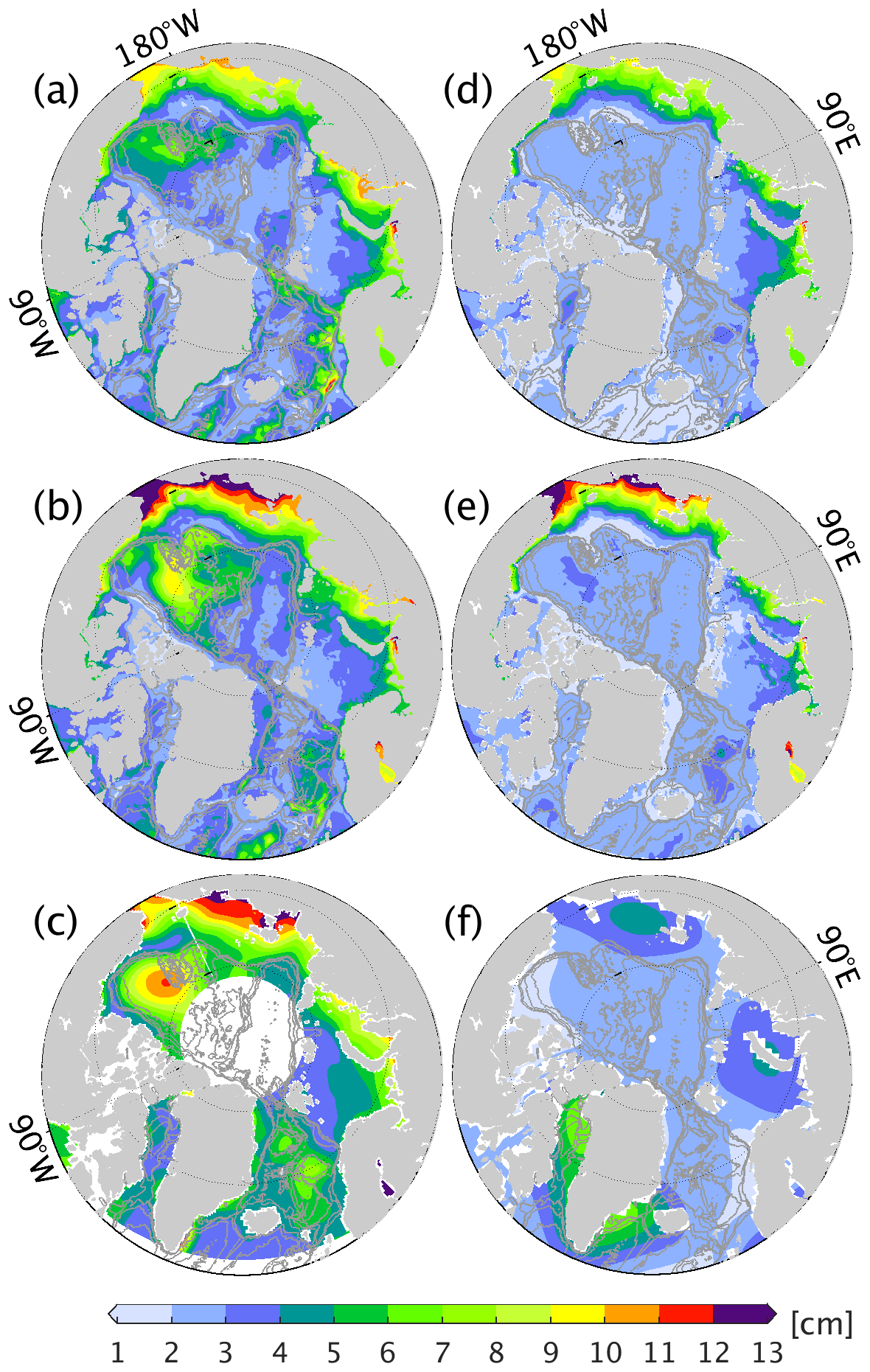
Figure 2 The rms variability of (a–c) sea level and (d–f) bottom pressure in (a, d) ATLARC08km, (b, e) ATLARC04km, (c) satellite altimetry, and (f) GRACE. We computed the rms variability using monthly data from January 2003 to December 2011. Bathymetry contours of 500, 1000, 2000, and 3000 m are drawn with gray lines.

Besides monthly to decadal variability of bottom pressure, both the model simulations and the in situ observations also demonstrate significant high-frequency bottom pressure anomalies (Fig. 3). Both model simulations correlate well with the observations (∼0.45–0.55) in the five shown locations, but ATLARC04km and ATLARC08km underestimate the rms variability by ∼30 %–50 %, with ATLARC04km showing relatively stronger rms variability.

Figure 3 Time series of bottom pressure anomalies in ATLARC08km, ATLARC04km, and in situ observations. Observations are derived from (a) mooring A, (b) mooring B, (c) mooring C, and (d) mooring D of BGEP. Panel (e) is from the North Pole Environmental Observatory (NEPO) moorings. Mooring locations are marked in Fig. 1.

The comparisons above indicate that the model simulations reasonably reproduce the observed sea level and bottom pressure variability at both high-frequency and low-frequency bands. In the following parts, we will use the daily output of ATLARC04km to reveal spatial variability of sea level at high frequency and seasonal periods and use the monthly output of ATLARC08km to explore the decadal sea level variability.

4 Sea level variability and its relation with bottom pressure and steric height

A model study (Proshutinsky et al., 2007) and satellite observations (Armitage et al., 2016) showed that the Arctic sea level presents distinctive seasonal to decadal variability. In situ bottom pressure observations also reveal energetic variability at submonthly frequencies. Here, we concentrate on sea level variability at very high frequency (<30 d), on the seasonal cycle, and at decadal timescales (>4 years).

At a period of < 30 d, rms variability of sea level up to 14 cm appears in the marginal seas and along the coasts (Fig. 4a), accounting for 60 %–80 % of the local sea level variance (Fig. 4d). The seasonal sea level variability is pronounced in the marginal seas and southern edge of the Beaufort Sea, and it explains 20 %–40 % of the total sea level variance. In the deep regions of the pan-Arctic Ocean, the decadal variability dominates the sea level variability, and it explains more than 70 %–90 % of the sea level variability. Overall, in the marginal seas, sea level variability is dominated by submonthly and seasonal signals. In contrast, decadal sea level variability dominates in the deep regions of the pan-Arctic Ocean. Besides, seasonal variability is also visible in the southern periphery of the Beaufort Sea, indicating possible exchanges between the marginal seas and the Beaufort Sea.

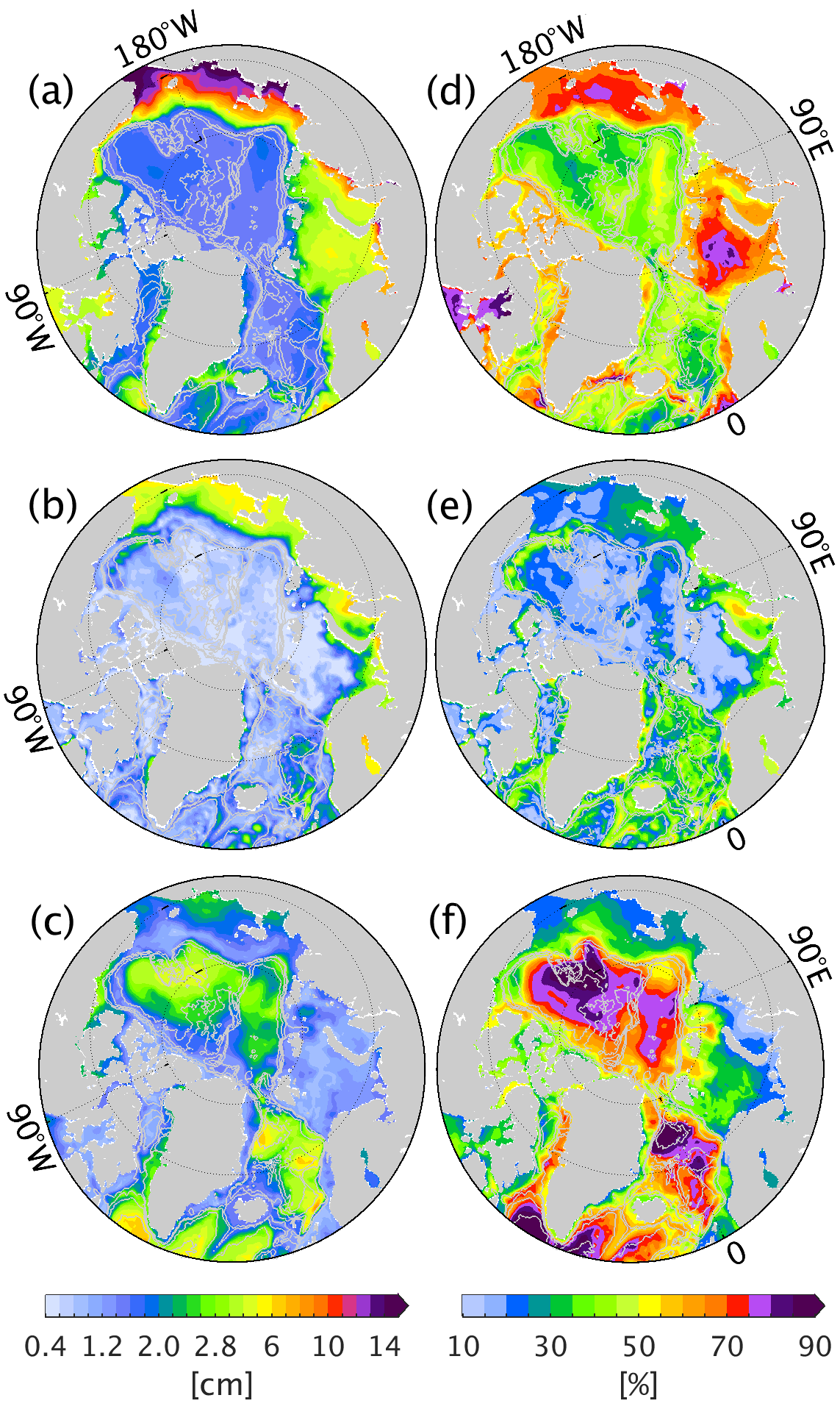
Figure 4 The rms variability (cm) of sea level (a) in the high-frequency band (<30 d), (b) at the seasonal cycle, and (c) at decadal periods (>4 years). Panels (d)–(f) are the corresponding ratios (%) to the total sea level variance that panels (a)–(c) explained. The high-frequency and seasonal variability (a, b, d, e) uses the daily output of ATLARC04km, and decadal variability (c, f) uses the monthly output from ATLARC08km. The gray lines denote bathymetry contours of 500, 1000, 2000, and 3000 m.

4.1 High-frequency (<30 d) variability

With a coarse resolution model simulation, Vinogradova et al. (2007) demonstrated that sea level variability is coherent with and virtually equivalent to bottom pressure in the midlatitude and subpolar regions at periods of < 100 d, reflecting the barotropic nature of high-frequency variability (Stammer et al., 2000). Here, we revisit the high-frequency sea level variability in the pan-Arctic Ocean with high-resolution model simulations and a transfer function (Vinogradova et al., 2007) of sea level and bottom pressure.

Except for the Norwegian Atlantic Current (NwAC) and the East/West Greenland Current (EGC/WGC), the amplitude of the transfer function between sea level and mass component is ∼1 (Fig. 5a) in most of the pan-Arctic regions. The phases (Fig. 5b) are ∼0 in the entire Arctic Ocean, indicating that the high-frequency sea level variability is mostly barotropic. However, in the strong current regions, including NwAC, EGC, and WGC, an amplitude of the transfer function of ∼0.4 is observed, revealing that both barotropic and baroclinic processes contribute to the high-frequency sea level variability.

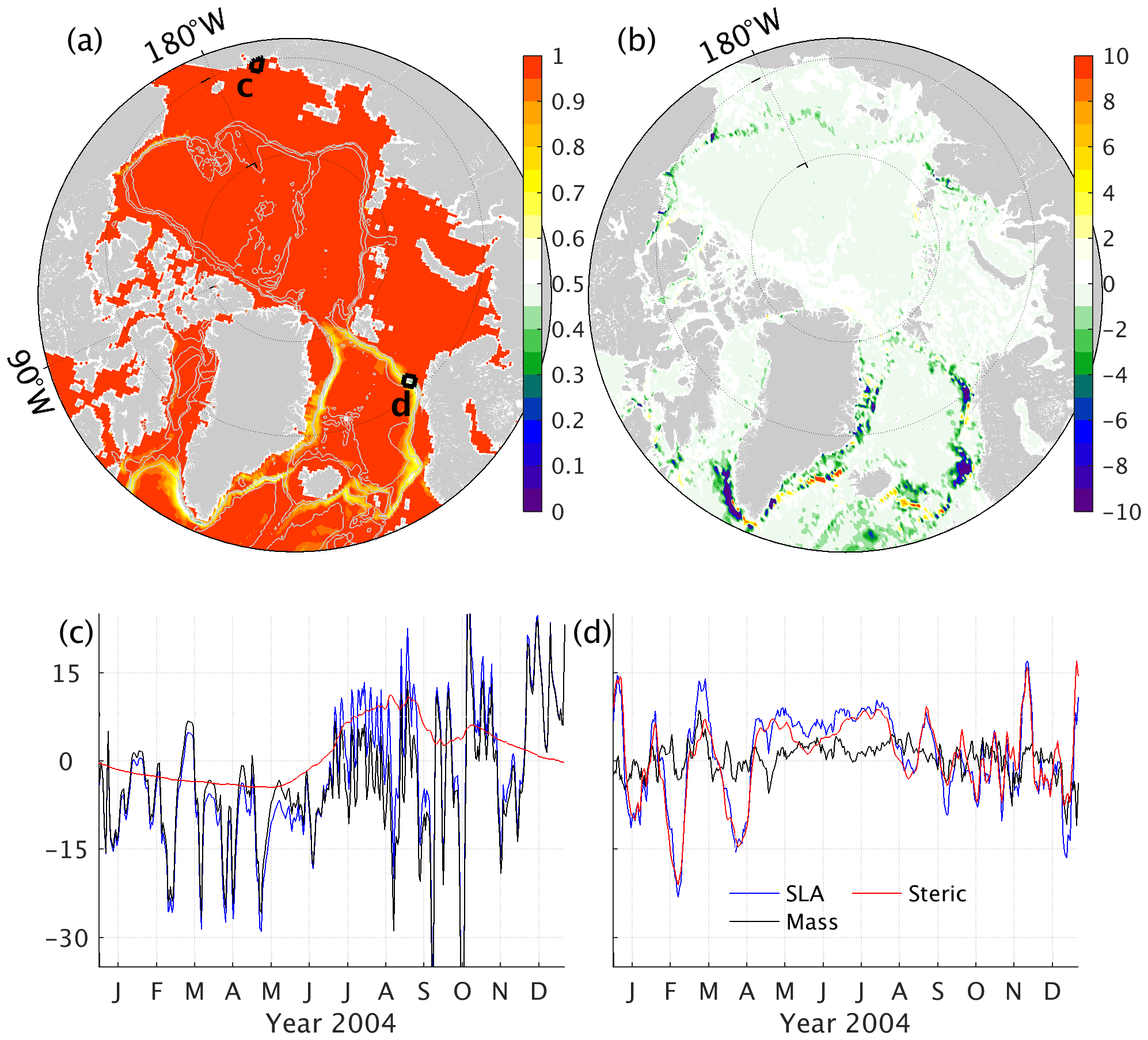
Figure 5 (a) Amplitude and (b) phase of the transfer function between sea level anomaly and bottom pressure anomaly at periods of < 30 d. Time series of sea level anomaly (blue lines), mass component (black lines), and steric component (red lines) averaged (c) in the East Siberian Sea (black box c in panel a) and (d) along the NwAC (black box d in panel a).

Subregions in the East Siberian Sea (c in Fig. 5a) near the maximum rms variability and along the NwAC (d in Fig. 5a) are used to reveal details of the high-frequency sea level variability. It is clear that the sea level anomaly in the East Siberian Sea (Fig. 5c) is almost equivalent to the bottom pressure anomaly, and the steric component contributes slightly to the seasonal timescale. Along the NwAC (Fig. 5d), pronounced steric height variability with timescales of 20–60 d is visible, which may be caused by baroclinic instability, and the mass component shows high-frequency variability.

The high-frequency sea level variability is mainly related to wind forcing (Fukumori et al., 1998) at high latitudes. Correlations to the wind forcing and sea level anomalies are used to explain the driving mechanisms of the high-frequency SLA variability. The negative correlations between high-frequency sea level variability and wind stress curl (shading in Fig. 6a) in the Canadian Basin and Greenland, Iceland and Norwegian (GIN) seas (−0.3) and in the marginal seas (−0.3 to −0.5) reveal that local sea level increase/decrease is partially related to wind-induced convergence/divergence (vectors and shading in Fig. 6a) of water. In addition, the high correlations of SLA to wind stress (vectors in Fig. 6a) along the coast reveal that cyclonic along-shore wind distributes water to the coast through Ekman transport, increasing sea level there.

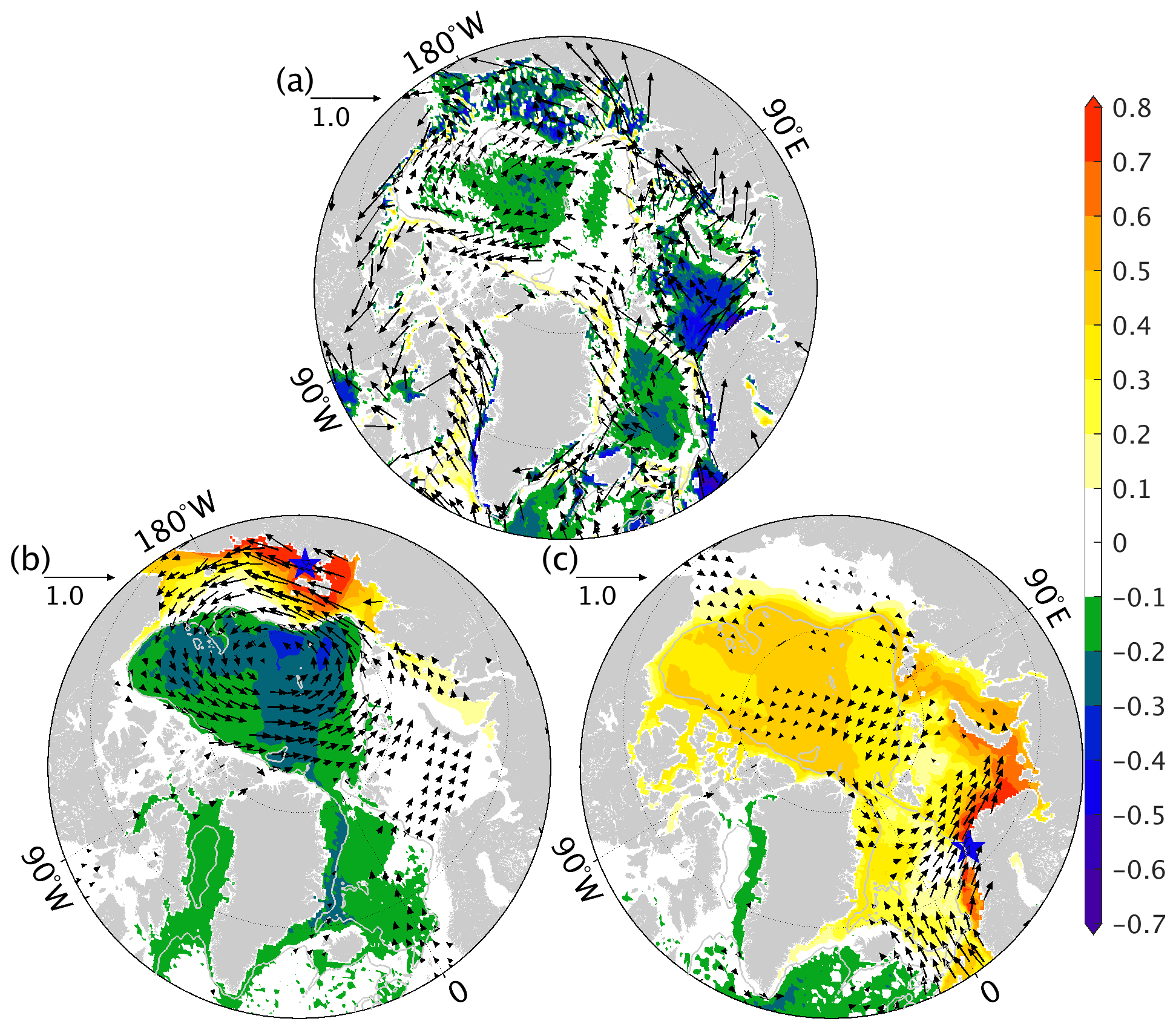
Figure 6 (a) Coefficients of the correlation between sea level anomalies and wind stress curl (shading), wind stress (vectors) at periods of < 30 d. (b) Correlations of sea level anomalies in subregions of the East Siberian Sea (blue star in panel b) to wind stress (vectors) and sea level anomalies (shading). Panel (c) is the same as panel (b) but for sea level anomalies in the Norwegian shelf (blue star in panel c). Correlation coefficients with 95 % significance levels are plotted.

To further explore the propagating features of the strong SLA variability along the coasts, we show correlations of SLA in subregions of the East Siberian Sea (blue star Fig. 6b) and Norwegian coast (blue star Fig. 6c) to SLA (shading) and wind stress (vectors). Figure 6b demonstrates that anticyclonic wind stress distributes water to the coast through Ekman transport which interacts with topography, raising coastal sea levels. SLA in the Norwegian coast is also driven by along-shore wind (vectors in Fig. 6c) through Ekman transport, and the SLA signals propagate along the coast to the Barents Sea and the central Arctic Ocean (shading in Fig. 6c).

Overall, both the model simulations and the several bottom pressure records demonstrate high-frequency bottom pressure variability in the Arctic Ocean (Fig. 3). The model simulations reveal that the high-frequency variability is barotropic primarily in response to wind-induced Ekman transport and propagations of the barotropic signals. In the strong current regions, steric effects also contribute to local sea level variability caused by baroclinic processes.

4.2 Seasonal variability

Seasonal sea level variability could be related to the redistribution of water from the deep ocean to the marginal seas due to cyclonic/anticyclonic wind stress (Proshutinsky and Johnson, 1997), a seasonal variation of the Arctic Ocean volume (Armitage et al., 2016). In addition, the steric effect due to warm Atlantic inflow and sea ice formation/melting contribute to regional sea level variability in the Barents Sea (Volkov and Landerer, 2013). This section focuses on the spatially varying Arctic sea level variability at seasonal periods and its mechanism.

Like the high-frequency sea level variability, the mass component still dominates the seasonal sea level variability in the marginal seas (Figs. 4b and 7a). Halosteric effects are significant near the river mouth, seasonal ice edge, and along the coast of Alaska (Fig. 7b), indicating the spreading of freshwater driven by oceanic flows. Pathways of freshwater from rivers and marginal seas to the Makarov Basin and the periphery of the Beaufort Sea can also be inferred from the significant halosteric effect. The thermosteric effects dominate the ice-free region in the GIN seas and the Barents Sea, and it is remarkably weakened as it penetrates the ice-covered Arctic Ocean (Fig. 7c).

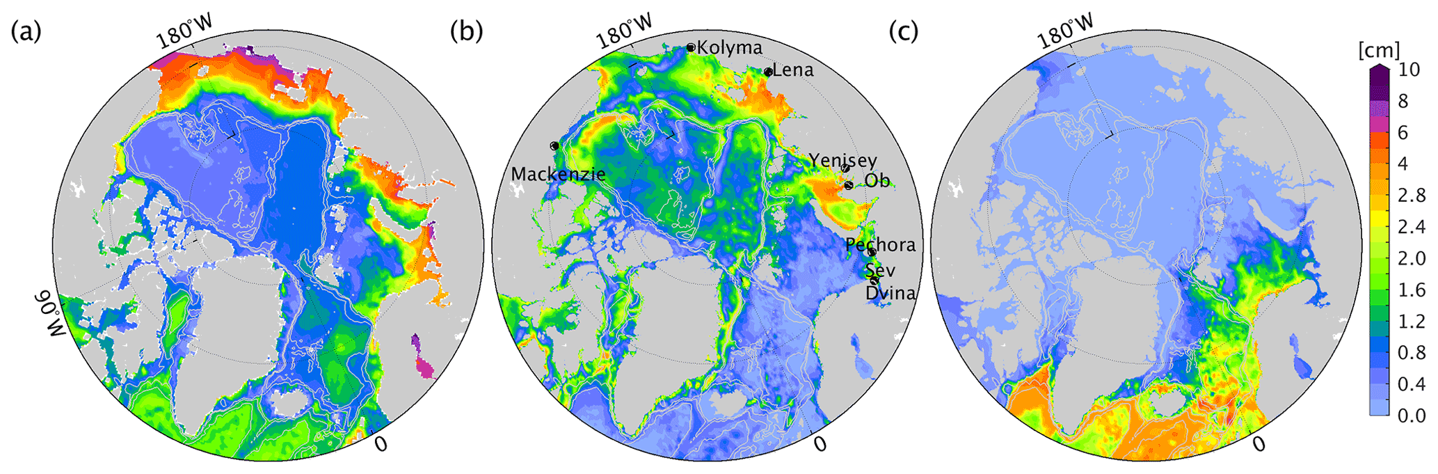
Figure 7 The rms variability of (a) mass, (b) halosteric, and (c) thermosteric components during the seasonal periods.

Sea level changes reflect total volume changes. The Arctic volume anomalies, dominated by mass component, shows a clear seasonal cycle overlaid with subseasonal variability (Fig. 8a). Since the surface freshwater flux is treated as a virtual salt flux, river runoff and evaporation minus precipitation do not change the total volume directly. The seasonal volume variability, especially the mass component, is driven by volume exchanges with the Pacific and Atlantic oceans. The steric component (red lines in Fig. 8), especially the halosteric component (magenta lines in Fig. 8), causes the volume to decrease in the winter season and increase in the summer season due to the sea ice formation/melting.

Figure 8 (a) Time series of total volume (VOL) anomaly in the Arctic Ocean (see Fig. 1 for the regions) and the contributions from mass changes (mass) and steric effects (steric). The halosteric component (halosteric) and the GRACE-observed mass component are also shown. Panels (b) and (c) show the corresponding values in (b) the deep basin (>500 m) and (c) the shallow water (<500 m).

The model simulates more substantial seasonal mass variability than the GRACE measurement. Still, it fails to reproduce the secondary peak from May to July (Fig. 8a), which may relate to river discharge in the marginal seas. Splitting the total Arctic volume changes into contributions from the deep basin and coastal seas, we note that the secondary peak is related to volume changes in the deep basin from May to July (Fig. 8b) in both the model simulation and the GRACE observations. At the same time, volume anomalies are negative in the marginal seas. This antiphase of the volume anomalies in the deep basin and marginal seas seems to be driven by the cyclonic/anticyclonic wind pattern in the summer/winter season (Proshutinsky and Johnson, 1997). Mean sea level anomalies from June to August (Fig. 9a) and from December to February (Fig. 9b) further reveal the antiphase of the sea level changes between the deep basin and the shallow waters. The mean pattern of wind stress anomalies (vectors in Fig. 9) indicates that wind-driven Ekman transport drives the water toward/away from the marginal seas, resulting in the antiphase of seasonal sea level variability in the deep basin and shallow waters.

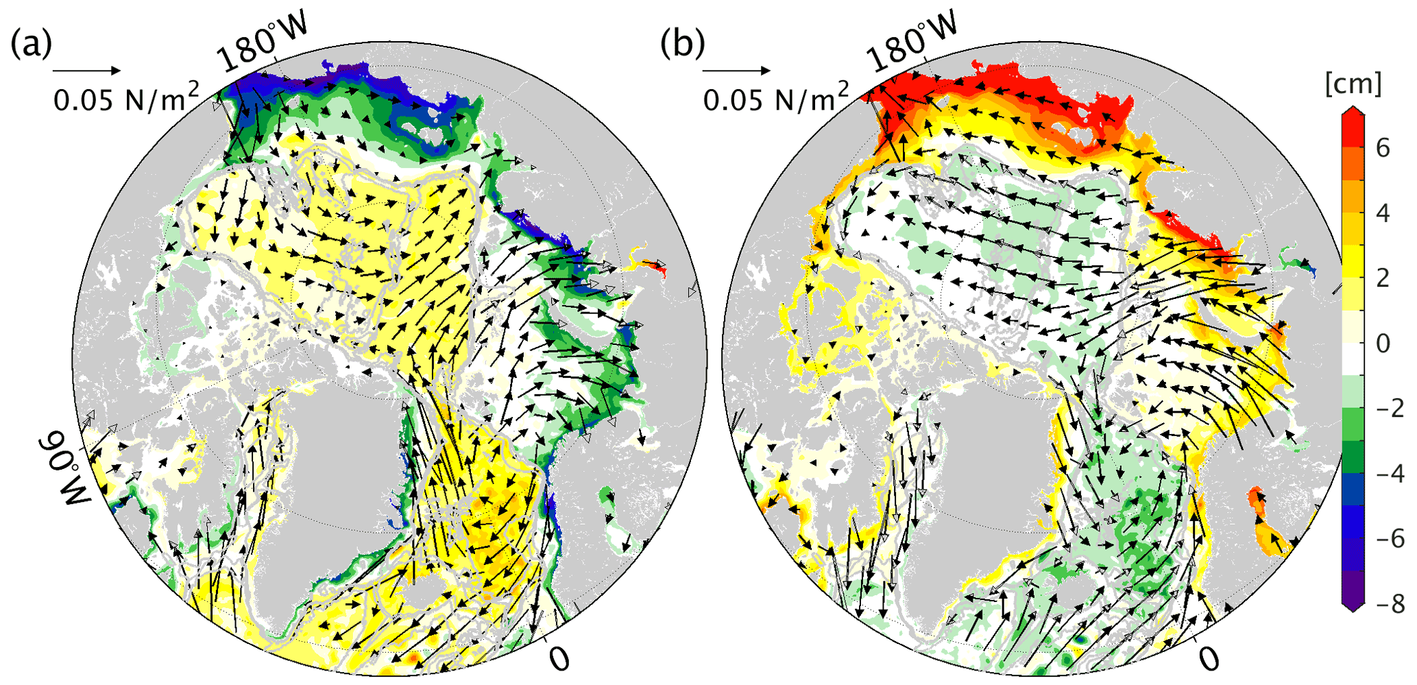
Figure 9 SLA (shading) and wind stress anomalies (vectors) to the climatology averaged from (a) June to August and (b) December to February. The daily output of ATLARC4km is used.

The model simulation demonstrates the critical importance of exchanges with the Pacific and Atlantic oceans for the Arctic volume changes at seasonal periods. The wind stress will further redistribute water in the Arctic Ocean, resulting in the antiphase pattern of sea level changes in the shallow waters and deep basins. Using a one-dimensional model, Peralta-Ferriz and Morison (2010) demonstrated that river runoff and evaporation minus precipitation (EmP) drive the basin-scale seasonal mass variation of the Arctic Ocean. This process is not included in our model simulations due to the virtual salt flux parameterization. But it should be noted that either input from river runoff and EmP (Peralta-Ferriz and Morison, 2010) or exchanges with the Pacific and Atlantic oceans are large enough to drive the Arctic volume changes. Moreover, the wind stress will further redistribute the water to different regions. It is also expected that volume input from the rivers (∼700 km³) could significantly alleviate the negative volume anomalies from May to August in the marginal seas.

4.3 Decadal variability

The Arctic sea level shows significant decadal variability driven by cyclonic/anticyclonic wind patterns (Proshutinsky and Johnson, 1997), accompanied by freshwater content changes (Häkkinen and Proshutinsky, 2004; Köhl and Serra, 2014). Satellite altimetry observations were used to infer Arctic freshwater content increases (Armitage et al., 2016; Giles et al., 2012; Proshutinsky et al., 2019; Rose et al., 2019) and complement freshwater content estimate using in situ observations (Haine et al., 2015; Polyakov et al., 2020; Rabe et al., 2011, 2014). This section examines the spatial variability of Arctic decadal sea level and addresses its relation to the mass, halosteric, and thermosteric components.

The ATLARC08km simulation revealed that the pronounced decadal sea level variability in the Canadian and Eurasian Basins (Fig. 4c) is mainly due to the halosteric effect (Fig. 10b), with the mass components accounting for 20 %–30 %. The thermosteric effect dominates in the GIN seas, mainly relating to the convection processes (Brakstad et al., 2019; Ronski and Budéus, 2005). Brakstad et al. (2019, see their Fig. A1) demonstrated that a change from shallow convection to deep convection can lead to temperature changes of more than −0.2 ^∘C over the upper 600 m and salinity changes of 0.02 PSU over the upper 200 m, resulting in a significant thermosteric effect. In the north Atlantic Ocean, the thermosteric effect dominates. At the same time, the halosteric effect compensates for the thermosteric effect in this region, rendering more considerable thermosteric height variability than decadal total sea level variability.

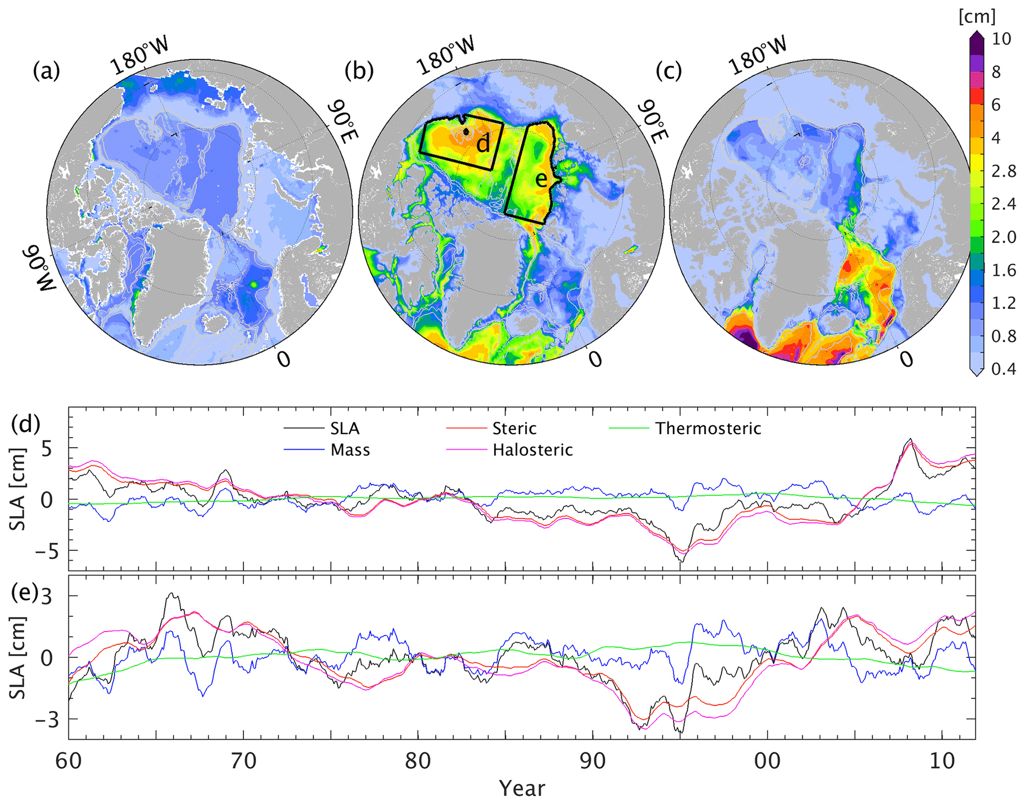
Figure 10 The rms variability at the decadal period of (a) bottom pressure anomaly, (b) the halosteric component, and (c) the thermosteric component. Panels (d) and (e) show the time series of sea level anomaly and mass, steric, and thermo-/halosteric components in the Canadian and the Eurasian basins (see the regions in panel b), respectively. Linear trends in all the time series are removed in panels (d) and (e).

Time series of sea level anomalies and their different components confirm that sea level variability is mostly halosteric in the Canadian (Fig. 10d, Armitage et al., 2016; Giles et al., 2012; Morison et al., 2012) and Eurasian basins (Fig. 10e), and that the thermosteric component contributes with a linear trend (not shown here). In addition, the mass components contribute to the interannual sea level variability (blue lines in Fig. 10d and e) in both the basins. We note that the mass changes are highly correlated in the Canadian and Eurasian basins (r>0.98 with 95 % significance level). They are positively correlated to the mass changes in the deep basin of the GIN seas and the Arctic Ocean and are negatively correlated to mass changes in the Arctic marginal shelves, especially in the East Siberian Sea, representing a barotropic response of sea level to changes of the intensity and locations of the Icelandic Low and the East Siberian High (e.g., Proshutinsky and Johnson, 1997). The halosteric component shows clearly decadal variability and is in phase with that in the Canadian Basin. The thermosteric component slightly compensates for the halosteric component.

5 Capability of the observing system to monitor freshwater content variability

Observing Arctic freshwater content changes remains challenging (Proshutinsky et al., 2019). The results above and previous studies (Giles et al., 2012; Morison et al., 2012; Proshutinsky et al., 2019) have indicated that satellite altimetry could infer freshwater content changes. International efforts try to enhance the profiles observing system, including ice-tethered profilers (ITPs, Toole et al., 2016, https://doi.org/10.7289/v5mw2f7x), shipboard observations, and moorings. Here, we test their capability to monitor the freshwater changes in an idealized setting in which (1) we do not consider influences of observational errors and (2) we assume the profiles sample the top 800 m and the moorings sample from 65–800 m. Freshwater inventory is defined, as in Rabe et al. (2011) and Schauer and Losch (2019), as the freshwater fractions relative to a conventional reference salinity S₀=34.8 PSU integrated over depth, and freshwater content is the total freshwater inventory over a region:

$$\begin{array}{}\text{(5)}& \mathrm{FWC}=\int \mathrm{FWId}A=\int \underset{H}{\overset{\mathrm{0}}{\int }}{\displaystyle \frac{S_{\mathrm{0}}-S}{S_{\mathrm{0}}}}\mathrm{d}z\mathrm{d}A,\end{array}$$

with H being the depth of the 34.8 PSU isohaline. The reference salinity indicates the mean salinity within the Arctic Ocean and can differ slightly in previous studies, which mainly impacts the mean state of freshwater content.

5.1 Satellite altimetry and GRACE measurements

Giles et al. (2012) used altimetric sea level observations, GRACE-based bottom pressure, and a static 1.5-layer model to infer freshwater changes in the Canadian Basin. They assumed that freshwater changes lead to sea level and isopycnal changes simultaneously, changing the water column's layer thickness and total mass. In this case, freshwater change in the water column is estimated as follows:

$$\begin{array}{}\text{(6)}& \begin{array}{rl}\mathrm{\Delta }FW& ={\displaystyle \frac{S_{\mathrm{2}}-S_{\mathrm{1}}}{S_{\mathrm{2}}}}\cdot \mathrm{\Delta }h={\displaystyle \frac{S_{\mathrm{2}}-S_{\mathrm{1}}}{S_{\mathrm{2}}}}\\ & \cdot \left({\mathit{\eta }}^{\prime }\cdot \left(\mathrm{1}+{\displaystyle \frac{{\mathit{\rho }}_{\mathrm{1}}}{{\mathit{\rho }}_{\mathrm{2}}-{\mathit{\rho }}_{\mathrm{1}}}}\right)-{\displaystyle \frac{\mathrm{\Delta }m}{{\mathit{\rho }}_{\mathrm{2}}-{\mathit{\rho }}_{\mathrm{1}}}}\right),\end{array}\end{array}$$

where ρ₁=1025.0 kg m⁻³ and ρ₂=1028.0 kg m⁻³ are the mean density in the top and bottom layers. S₁=33.0 PSU is the mean salinity in the top layer, and S₂=34.8 PSU is a reference salinity. η^′ and Δm are the sea level anomaly and bottom pressure anomalies observations. Morison et al. (2012) suggest that freshwater changes depend on steric height changes linearly and could be approximated by:

$$\begin{array}{}\text{(7)}& \mathrm{\Delta }FW=\mathit{\alpha }\cdot {\mathit{\eta }}_{\mathrm{s}}^{\prime },\end{array}$$

where α is an empirical constant estimated from in situ profile observations and is set to 35.6 following Morison et al. (2012). The choice of α just contributes a static offset to freshwater content estimation in Eq. (7).

In the Canadian Basin, freshwater content changes and the two estimates show similar decadal variabilities, but differences remain in the seasonal and long-term trends (Fig. 11a and b). Since the halosteric effect dominates the steric effect, estimation using Eq. (7) matches the seasonal freshwater cycle well (red and black lines), considering the amplitude and phase. However, it overestimates the long-term trend (Fig. 11b) since Eq. (7) attributes the thermosteric effect to freshwater changes. Equation (6) infers a much more substantial seasonal variability of freshwater content, and the phase does not always match the real freshwater content changes (blue and black lines).

Figure 11 (a) Freshwater content anomalies (10³ km³) and approximated based on Eq. (6) in blue and Eq. (7) in red using the monthly output of ATLARC08km. The thick dashed lines are the annual mean values. (b) The differences of the approximated annual mean freshwater content anomalies based on Eq. (6) in blue and Eq. (7) in red to the annual mean freshwater content anomalies.

Equation (6) assumes the upper layer adjusts simultaneously with sea level anomaly, which may not apply in the presence of baroclinic effects. To illustrate the limitation of Eq. (6), we take the differences between February 2003 and September 2002 (in which Eq. 6 fails to reproduce the phase and the amplitude of freshwater content changes) and between 2008–2010 and 1994–1996 (when Eq. 6 reproduces the freshwater changes well).

From September 2002 to February 2003 (Fig. 12a), anticyclonic wind stress anomalies occur in the Beaufort Sea, resulting in positive SLA through Ekman transport. However, freshwater content is reduced during this period. The salinity difference averaged over the central Arctic Ocean reveals that salinity increases in the top 30 m were caused by ice formation. At the same time, the isopycnal (27.9 kg m⁻³) did not deepen (Fig. 12c) as predicted by Eq. (6). The assumption that freshwater content changes are captured by freshwater column thickness changes $\mathit{\eta }\cdot \left(\mathrm{1}+\frac{{\mathit{\rho }}_{\mathrm{1}}}{{\mathit{\rho }}_{\mathrm{2}}-{\mathit{\rho }}_{\mathrm{1}}}\right)$ (dashed red lines in Fig. 12c) fails to infer freshwater content changes in this case.

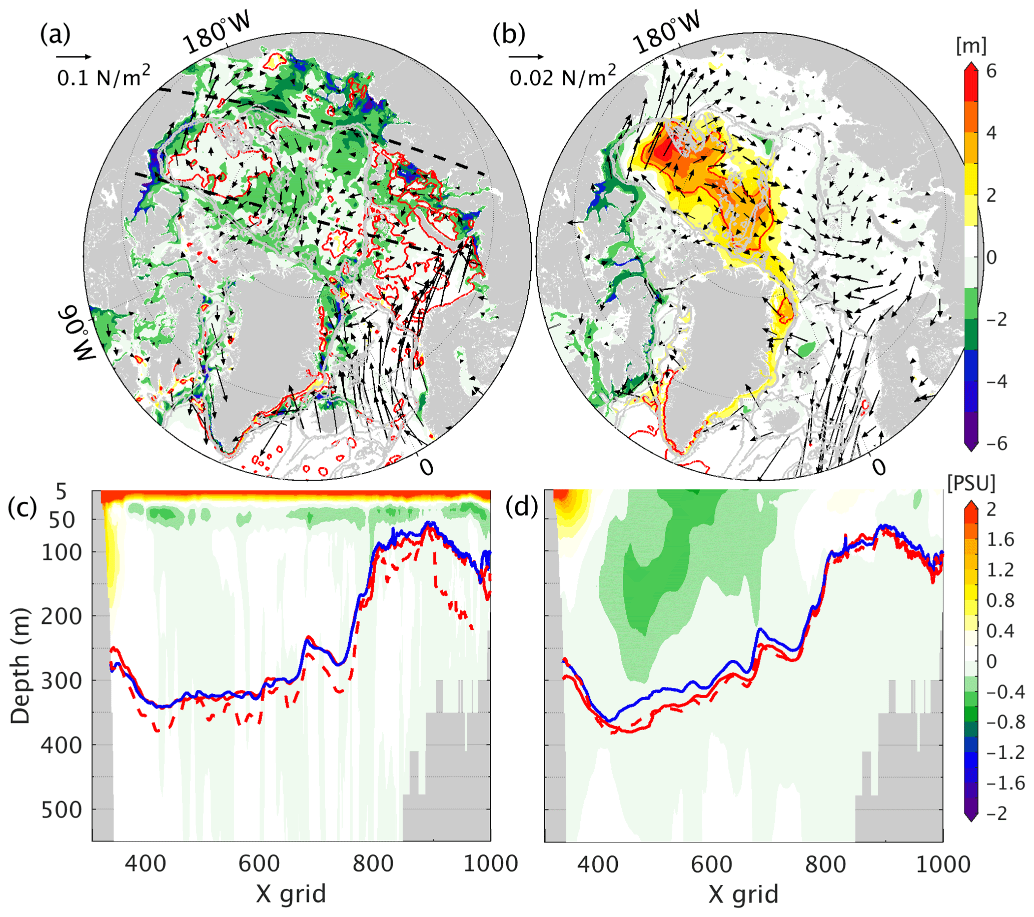
Figure 12 The differences of freshwater inventory in meters (shading), sea level anomaly (0.15 m contour, black lines), and wind stress (vectors) between (a) February 2003 and September 2002, and (b) 2008–2010 and 1994–1996. Panels (c) and (d) are the corresponding salinity differences (shading) average over the central Arctic Ocean (dashed black lines in panel a). The blue lines denote the 27.9 kg m⁻³ isopycnal in September 2002 and 1994–1996, respectively. The red lines and dashed red lines are the 27.9 kg m⁻³ isopycnal and the diagnosed 27.9 kg m⁻³ isopycnal with SLA and Eq. (5) in February 2003 and 2008–2010, respectively.

From 1994–1996 to 2008–2010, anticyclonic wind stress anomalies appeared in the Canadian Basin, accompanied by positive SLA and freshwater content anomalies (Fig. 12b). During that period, Ekman pumping deepens the isopycnals (blue and red lines in Fig. 12), accumulating more freshwater and reducing the local salinity over the top 300 m (Fig. 12d). In this scenario, the water column thickness change dominates the freshwater content variability, which is approximated by $\mathit{\eta }\cdot \left(\mathrm{1}+\frac{{\mathit{\rho }}_{\mathrm{1}}}{{\mathit{\rho }}_{\mathrm{2}}-{\mathit{\rho }}_{\mathrm{1}}}\right)$ (dashed red lines in Fig. 12d). Therefore, Eq. (6) captures the interannual freshwater content changes using satellite altimetric observations. Caution needs to be taken when inferring Arctic Ocean freshwater content changes using satellite altimetry observations and GRACE measurements. In addition, Fig. 12b and d indicate that Eq. (6) can be only used in the Canadian Basin where wind drives the sea level changes and the deepening/shoaling of the isopycnals.

5.2 In situ profilers

In situ profilers measure salinity directly, but they are limited by sea ice and distributed unevenly in time and space. Over the past decades, the endeavor of polar expeditions and the evolving measurement techniques (e.g., ITP) have generated a large number of hydrographic data in the central Arctic and subarctic seas (e.g., Behrendt et al., 2018). Using historical hydrographic observations and objective mapping techniques, previous studies (e.g., Haine et al., 2015; Polyakov et al., 2008; Rabe et al., 2011, 2014) have explored Arctic freshwater content changes and the mechanisms on multi-year periods. However, the interpolated products suffer from high uncertainties at timescales shorter than multi-year periods (e.g., Fig. 4 in the Supplement of Rabe et al., 2014), indicating observational gaps on resolving the seasonal to interannual freshwater content changes. Besides, spatial observational gaps are observed (e.g., Fig. 7 in Rabe et al., 2011) but not explored yet. This section examines how existing hydrographic observations could help reveal Arctic freshwater content changes and identify observational gaps in time and space. Based on the spatiotemporal distribution of profiles compiled by Behrendt et al. (2018) and an ensemble optimal interpolation (EnOI) scheme (Evensen, 2003; Lyu et al., 2014), we test to what extent the generated synthetic profiles could help to reconstruct the “true” state (here the ATLARC08km simulation) during the period 1992 to 2012. Details of the EnOI scheme are given in Appendix A.

As shown in Fig. 13, the sparse in situ profiles help bring the freshwater inventory in the background state close to the “truth” state. However, it was not until 2007 that the reconstructed state reproduces the seasonal to interannual freshwater inventory variability in the Canadian Basin, benefiting from the increasing number of research activities and international collaborations. We further examined rms errors of freshwater inventory from 1992–2006 (Fig. 14a), 2007–2012 (Fig. 14b) and the corresponding profile locations (Fig. 14c and d). The lack of in situ profiles in the Arctic shelves (Fig. 14c and d) and in the deep basin from 1992–2006 (Fig. 14c) results in pronounced errors. The ITP profiles (trajectories in Fig. 14d) enhanced the capability to observe the Arctic freshwater changes in the deep basin and the winter season, significantly reducing freshwater inventory uncertainties (Fig. 14b). Additionally, high errors remain in regions with high variability (e.g., EGC/WGC), in the Laptev Sea and the Alaskan coast, extending from the coasts to the deep basin, underlining the observing requirements.

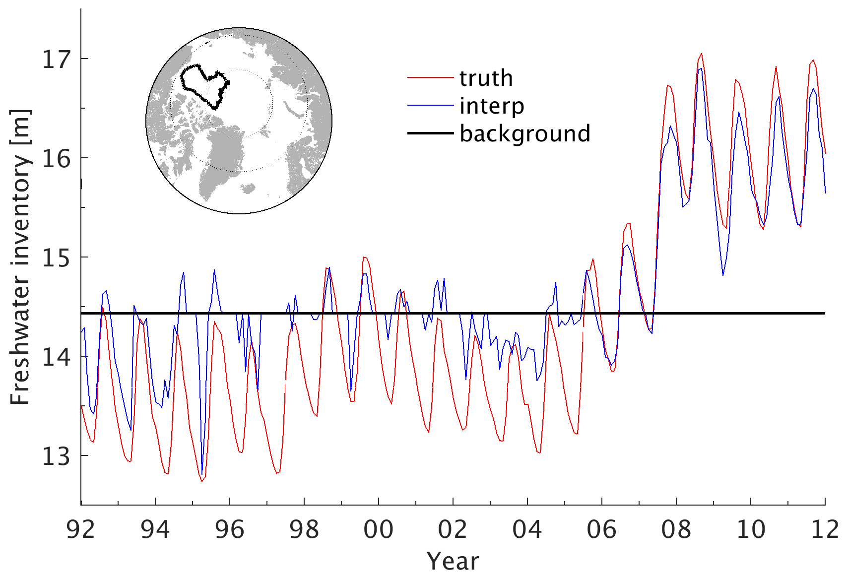
Figure 13 Mean freshwater inventory (in meter) in the Canadian Basin (enclosed by the black line in the top subplot) from the background state, the “truth”, and the optimal interpolation reconstructed state (see legend).

Figure 14 Root mean square errors of freshwater inventory (in meter) between the reconstructed state and the “truth” from (a) 1992–2006 and (b) 2007–2012. Panels (c) and (d) are the corresponding profile locations in different months (color bar).

The above results highlight that the increase of hydrographic observations has enhanced our ability to reconstruct the changes in Arctic freshwater content since 2007. A lack of hydrographic observations in the coastal areas results in significant errors in the marginal seas, which require extensive international collaborations.

6 Summary and conclusions

Sea level variability reflects changes in ocean dynamics, atmospheric forcing, and terrestrial runoff processes (Stammer et al., 2013). In particular, sea level observations have been applied to infer freshwater content changes (Armitage et al., 2016; Giles et al., 2012; Proshutinsky et al., 2019) in the central Arctic Ocean. To complement our understanding of the Arctic sea level variability and its mechanisms, we use two high-resolution ATLARC model simulations to investigate the Arctic sea level variability at different timescales and the relation with bottom pressure and thermo-/halosteric effects, identifying critical observational gaps that need to be filled.

Both the model simulations and mooring observations reveal very high-frequency bottom pressure variations. The model simulations confirm that the bottom pressure anomaly is equivalent to sea level anomaly in most areas of the Arctic Ocean at periods of < 30 d, reflecting the barotropic nature of this high-frequency variability. Correlation analyses show that the high-frequency sea level variability is caused by wind-driven Ekman transport and propagations of these barotropic signals.

The seasonal sea level variability is dominated by volume exchanges with the Pacific and Atlantic oceans and the redistribution of the water by wind stress. Halosteric effects due to river runoff and ice melting/formation are also pronounced in the marginal seas and seasonal sea ice extent regions. Peralta-Ferriz and Morison (2010) demonstrated that river runoff and EmP drive the seasonal cycle of the Arctic bottom pressure. Although the virtual salt flux parameterization could not mimic the influences of volume input from rivers and surface fluxes, the model simulations still simulate much stronger seasonal mass anomalies than the observations from GRACE. Either volume exchanges with the Pacific and Atlantic oceans or volume input from river runoff and EmP are large enough to cause the Arctic Ocean's seasonal volume variability. They should work together, resulting in the Arctic seasonal volume variability. We speculate that using river runoff and EmP as volume flux, rather than the virtual salt flux, could likely improve the volume and sea level variability in the marginal seas from April to July since the volume inputs from river runoff could alleviate the negative volume anomalies in the marginal seas caused by wind.

At decadal timescales, the model simulations further confirm that the pronounced sea level variability in the central Arctic Ocean, especially in the Canadian Basin, is mainly a halosteric effect. Using the satellite altimetric observations and GRACE observations, the method of Giles et al. (2012) could infer the freshwater content changes in the Canadian Basin reasonably at timescales longer than one year since the upper layer (indicated by the 27.9 kg m⁻³ isopycnal in this study) requires time to adjust to sea level changes. Inferring freshwater content changes using a linear relation of freshwater content and steric height (Morison et al., 2012) reveals both the interannual and the seasonal variability of freshwater content. However, caution needs to be taken since the method attributes the thermosteric effects to halosteric effects, resulting in an additional linear trend. In addition, uncertainties in the satellite altimetric and GRACE measurements make the estimation more complicated and introduce significant uncertainties in the steric effects and freshwater content estimation (Ludwigsen and Andersen, 2021).

The increasing number of international collaborations and new measurement techniques have generated a large number of profiles. Previous studies have applied different objective mapping methods (Haine et al., 2015; Polyakov et al., 2008; Rabe et al., 2011, 2014) to reconstruct the Arctic freshwater content changes and budget. However, the interpolated products still show high errors for the annual mean estimate of freshwater content, indicating potential observational gaps in resolving the seasonal freshwater content cycle. We further examined the observational gaps in time and space using monthly output from ATLARC08km. Through reconstructing the salinity with synthetic observations, we note that the in situ profile system seems to capture the seasonal freshwater variability since the year 2007, encouraging further Arctic data synthesis studies (Behrendt et al., 2018; Cheng and Zhu, 2016; Steele et al., 2001) with more complicated interpolation methods. In addition, international collaborations need to be enhanced to fill in the observational gaps in the marginal seas. Further observing system simulation experiments (e.g., Lyu et al., 2021; Nguyen et al., 2020) should be performed in a coordinated fashion to develop an autonomous Arctic observing system (Lee et al., 2019; Sandu et al., 2021) to meet the societal and scientific needs.

Appendix A: An EnOI scheme

We use an EnOI scheme (Cheng and Zhu, 2016) to reconstruct the salinity in the Arctic Ocean using synthetic observations. At one grid (denoted by subscript “g”), the analysis state ${\mathit{\phi }}_{\mathrm{g}}^{\mathrm{a}}$ is a linear combination of a background field ${\mathit{\phi }}_{\mathrm{g}}^{\mathrm{b}}$ and surrounding in situ observations d:

$$\begin{array}{}\text{(A1)}& {\mathit{\phi }}_{\mathrm{g}}^{\mathrm{a}}={\mathit{\phi }}_{\mathrm{g}}^{\mathrm{b}}+K\left(d-H{\mathit{\phi }}_{\mathrm{g}}^{\mathrm{b}}\right)\cdot e^{-\frac{x^{\mathrm{2}}}{\mathrm{2}{\mathit{\sigma }}^{\mathrm{2}}}},\end{array}$$

where H is a transfer matric that maps model state from model space to observation points. In this study, the background state of salinity ${\mathit{\phi }}_{\mathrm{g}}^{\mathrm{b}}$ is taken as the mean salinity at each grid over the period 1992–2012. K is the Kalman gain, calculated as

$$\begin{array}{}\text{(A2)}& K={\mathit{\phi }}_{\mathrm{g}}^{\prime }\mathit{\phi }{{}^{\prime }}_{\mathrm{g}}^{\mathrm{T}}{H}^{\mathrm{T}}{\left(H{\mathit{\phi }}_{\mathrm{g}}^{\prime }\mathit{\phi }{{}^{\prime }}_{\mathrm{g}}^{\mathrm{T}}{H}^{\mathrm{T}}+\mathit{\gamma }{\mathit{\gamma }}^T\right)}^{-\mathrm{1}}.\end{array}$$

The superscript “T” denotes matrix transposition. In this formulation, we use ${\mathit{\phi }}_{\mathrm{g}}^{\prime }$, the salinity deviation from the mean salinity, to compute the error covariance of the background state (${\mathit{\phi }}_{\mathrm{g}}^{\prime }\mathit{\phi }{{}^{\prime }}_{\mathrm{g}}^{\mathrm{T}}$). We use monthly data from the years 1992 to 2012 to compute φ^′, resulting in a total of 252 ensemble members. For simplicity, we assume the representation errors γ only depend on depth, ranging from 0.09 PSU at the surface to 0.02 PSU in the deep ocean, and are not correlated.

The use of ensemble members to approximate the background error covariance (${\mathit{\phi }}_g^{\prime }\mathit{\phi }{{}^{\prime }}_g^{\mathrm{T}}$) will inevitably introduce long-distance correlations and propagate the observational information incorrectly over a much longer distance. Therefore, we introduce a Gaussian function depending on the distance between observational locations and the model grid (x in Eq. A1) and a decorrelation radius (σ in Eq. A1) to ensure that only observations within the decorrelation radius σ of a model grid point could modify the analysis state.

Taking the “true” salinity state from August 1992 and observation locations from 2008 (black dots in Fig. A1a), we test the impacts of the decorrelation radius on the analysis field. The background state is more saline than the truth (Fig. A1a). With a 300 km decorrelation radius (Fig. A1b), the analysis state reduces the errors near the observations while significant errors remain in regions far from observations. Increasing the decorrelation radius to 1000 km, we see that salinity errors in the marginal seas, North Pole areas, and Baffin Bay are reduced (Fig. A1c). A 2400 km decorrelation radius further reduces salinity error in the Canadian Arctic Archipelago (Fig. A1d). However, only slight improvements are observed in the central Arctic Ocean, and errors in the Kara Sea are slightly increased. Since we focus on the Arctic freshwater content variability, we use a 1000 km decorrelation radius throughout this study.

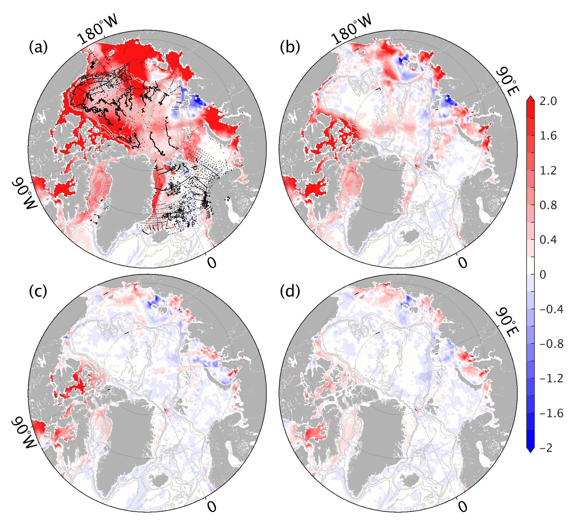
Figure A1 Example of sea surface salinity difference between (a) the background and the truth, (b) the analysis with a decorrelation radius of 300 km and the truth, (c) the analysis with a decorrelation radius of 1000 km and the truth, and (d) the analysis with a decorrelation radius of 2400 km and the “truth”. Black dots in panel (a) denote the locations of synthetic observations, sampled using sites of the observations from the year 2008.