The capabilities of Sentinel-MSI (2A/2B) and Landsat-OLI (8/9) in seagrass and algae species differentiation using spectral reflectance

This paper assesses the reflectance difference values between the respective spectral bands in the visible and near-infrared (VNIR) of Sentinel 2A/2B Multi-Spectral Instrument (MSI) and Landsat 8/9 Operational Land Imager (OLI) sensors for seagrass, algae, and mixed species discrimination and monitoring in a shallow marine environment southeast of Bahrain Island in the Arabian Gulf. To achieve these, a field survey was conducted to collect samples of seawater, underwater sediments, seagrass (Halodule uninervis and Halophila stipulacea), and algae (green and brown). In addition, an experimental mode was established in a goniometric laboratory to simulate the marine environment, and spectral measurements were performed using an Analytical Spectral Devices (ASD) spectroradiometer. Measured spectra and their transformation using the continuum-removed reflectance spectral (CRRS) approach were analyzed to assess spectral separability among separate or mixed species at varying coverage rates. Afterward, the spectra were resampled and convolved in the solar-reflective spectral bands of MSI and OLI sensors and converted into water vegetation indices (WVIs) to investigate the potential of red, green, and blue bands for seagrass and algae species discrimination. The results of spectral and CRRS analyses highlighted the importance of the blue, green, and near-infrared (NIR) wavelengths for seagrass and algae detection and likely discrimination based on hyperspectral measurements. However, when resampled and convolved in MSI and OLI bands, spectral information loses the specific and unique absorption features and becomes more generalized and less precise. Therefore, relying on the multispectral bandwidth of MSI and OLI sensors, it is difficult or even impossible to differentiate or to map seagrass and algae individually at the species level. Instead of the red band, the integration of the blue or the green band in WVI increases their power to discriminate submerged aquatic vegetation (SAV), particularly the water adjusted vegetation index (WAVI), water enhanced vegetation index (WEVI), and water transformed difference vegetation index (WTDVI). These results corroborate the spectral and the CRRS analyses. However, despite the power of blue wavelength to penetrate deeper into the water, it also leads to a relative overestimation of dense SAV coverage due to more scattering in this part of the spectrum. Furthermore, statistical fits (p<0.05) between the reflectance in the respective VNIR bands of MSI and OLI revealed excellent linear relationships (R² of 0.999) with insignificant root mean square difference (RMSD) (≤ 0.0015). Important agreement (0.63 ≤ R² ≤ 0.96) was also obtained between respective WVI regardless of the integrated spectral bands (i.e., red, green, and blue), yielding insignificant RMSD (≤ 0.01). Accordingly, these results pointed out that MSI and OLI sensors are spectrally similar, and their data can be used jointly to monitor accurately the spatial distribution of SAV and its dynamic in time and space in shallow marine environments, provided that rigorous data pre-processing issues are addressed.

1 Introduction

Seagrass meadows are identified as an important key for the characterization of environmental resources in estuarine and shallow coastal areas, and a fundamental health index allowing the assessment of coastal ecosystems. The composition and density of their species depend largely on water depth, temperature, salinity, coastal substrate material, and light penetration (Dierssen et al., 2015). Adapted to grow in shallow seawater down to a depth of 20 m, where approximately only 11 % of surface light reaches the bottom (Duarte and Gattuso, 2008), they play an essential role in the sustainability of global ecosystem biodiversity in most shallow nearshore areas around the world (Den-Hartog, 1970; Konstantinos et al., 2016). Moreover, the biodiversity of seagrass provides secure habitat and food for a wide variety of marine microorganisms, improves the quality of water, and protects shorelines against erosion in the middle and lower intertidal and subtidal zones (Roelfsema et al., 2009; Anders and Lina, 2011; Yang and Yang, 2012; Morrison et al., 2014). Like other vegetation cover, seagrass beds play an important role in carbon storage (Novak and Short, 2014), as well as effective removal of carbon dioxide from the “biosphere–atmosphere” system, which significantly mitigates the climate change impacts (Duarte et al., 2013; Lyimo, 2016). Although they occupy only 0.2 % of the world's oceans (Traganos, 2020), seagrass beds can store twice as much per unit area as forests and sequester around 10 % of the total carbon received by the oceans (Fourqurean et al., 2012).

Unfortunately, natural and anthropogenic disturbances and disasters have led to the decline of seagrass around the world (Green and Short, 2003; Orth et al., 2006; Grech et al., 2012; Wood, 2012) at local and regional scales. Undoubtedly, these causes substantially destroy the seagrass beds and biota associated in such habitats and unbalance the ecological functions of coastal zones. Short et al. (2011) showed that seagrass habitat disappeared worldwide at a rate of 110 km² per year between 1980 and 2006. Hence, understanding the spatial distribution of seagrass biomass, its extent, condition, and change over time is essential for its monitoring, management, and protection (Short and Coles, 2001; Waycott et al., 2009). Such monitoring provides updated and accurate information useful for the protection of several ecosystems (Leleu et al., 2012), conservation (Hamel and Andréfouët, 2010), coastal risk assessment (Warren et al., 2016), ecological resources development (Boström et al., 2011), and marine spatial planning (Saarman et al., 2012; Kibele, 2017). In addition, mapping and inventorying the total aboveground biomass of seagrass and algae are important for ecosystem health assessment (Short and Wyllie-Echeverria, 1996), alteration and dynamics in space–time (Neckles et al., 2012), biomass productivity and its contribution to the global biosphere carbon sink capacity (Waycott et al., 2009), and understanding the impacts of climate change (Hashim et al., 2014).

In the Arabian Gulf, the extreme environmental conditions combined with major seasonal variations in the marine environment promote the development of three seagrass species including Halodule uninervis which is the most dominant species, Halophila stipulacea that is less common, and Halophila ovalis, which is widely scattered and rarely forms relatively dense meadows. Along the western coast of the Arabian Gulf, these three species are reported and several species of marine algae are described, especially green and brown algae (Erftemeijer and Shuail, 2012). This natural resource is located in shallow waters with depths ranging from the intertidal zone to 20 m, supporting the second largest population of dugongs (Dugong dugon) in the world (Preen, 2004); as well as a large population of green turtles (Chelonia mydas) and hawksbill turtles (Eretmochelys imbricata) (Marshall et al., 2020). Unfortunately, these coastal ecosystems are under continuous threats from anthropogenic activities (Waycott et al., 2009), such as reclamation and dredging where several coastal developmental projects are constructed and others under construction (small islands projects development), industrial effluents, oil exploration, pipeline laying, maritime transportation, intensive circulation of commercial fishing boats, pollution and discharges of seawater desalinization and wastewater into the sea (Onuf, 1994; Dunton and Schonberg, 2002; Burfeind and Stunz, 2006; Naser, 2011; Erftemeijer and Shuail, 2012). Eventually, these activities catalyze the degradation and destruction of seagrass species and related ecosystems. Therefore, the assessment of seagrass conditions associated with a broad scale of benthic species should be based on relevant and accurate information to measure several health indicators of coastal areas to ensure the sustainable development of these natural resources.

Previously, photo interpretation approaches based on aerial photography have been adopted to follow seagrass and algae species development and assessment in space and time (Ferguson and Wood, 1990; Meehan et al., 2005; Mount, 2007). Afterward, the first generation of satellite remote sensing was used to investigate the seagrass classes' composition, differentiation, classification, etc. (Hossain et al., 2014; Komatsu et al., 2020). Unfortunately, these goals were difficult to achieve accurately because the radiometric and spectral resolutions of sensors lacked the sensitivity to discriminate among different marine vegetation species and fragmented classes (Mumby et al., 1997; Wicaksono and Hafizt, 2013). To improve land–water surface reflectivity and information extraction, recent developments in remote sensing science and technology have led to an improvement of sensors performance in spatial and spectral resolutions, assuming a potential mapping of the marine environment and aquatic vegetation at the species level; obviously, if species under investigation have distinct spectral signatures. For instance, the Multi-Spectral Instrument (MSI) aboard Sentinel 2A and 2B, as well as the Operational Land Imager (OLI) sensors aboard Landsat 8 and 9 platforms were designed with a significant improvement of the signal-to-noise ratio (SNR) and radiometric performances (Knight and Kvaran, 2014). The availability of this new generation of sensors offers innovative opportunities for long-term high-temporal frequency for Earth surface observation and monitoring (Mandanici and Bitelli, 2016). The free availability of their data significantly advances the applications of remote sensing with medium spatial resolutions (Roy et al., 2014; Wulder et al., 2015; Zhang et al., 2018). Thanks to the improvement of their spectral, radiometric, and temporal resolutions, they can expand the range of their applications to several natural resources and environmental domains for monitoring, assessing, and investigating (Hedley et al., 2012a, b). Moreover, the orbits of these four satellites' constellation (Sentinel 2A and 2B and Landsat 8 and 9) are designed to ensure a revisiting interval time of less than 2 d (Li and Roy, 2017; Li and Chen, 2020), thereby substantially increasing the monitoring capabilities of the Earth's surface and ecosystems (Drusch et al., 2012). Their spectral resolutions and configurations are designed in such a way that there is a significant match between the homologous spectral bands, i.e., closely related spectral filters position and bandwidths (Drusch et al., 2012; Irons et al., 2012). However, depending on the sensitivity of the intended application (Flood, 2017), the sensor radiometric drift calibration (Markham et al., 2016), the atmospheric corrections (Vermote et al., 2016), the surface reflectance anisotropy (Roy et al., 2017), and the sensors' co-registration (Skakun et al., 2017; Yan et al., 2018), it is plausible that the natural surface reflectances recorded by MSI and OLI sensors over the same target in the marine environment may be different. In addition, the relative spectral response profiles characterizing the filters (spectral responsivities) of these instruments are not perfectly identical between the homologous bands, so some differences are probably expected over the recorded land or water surface reflectance values, and therefore their data cannot be reliably used together (Bannari et al., 2004; Van-derWerff and Van-der-Meer, 2016; Bannari, 2019). The importance of these differences depends on the application (spectral characteristics of the observed target) and on the approach adopted to perform time-series analyses, mapping, or change detection exploiting these instruments (Flood, 2017). For instance, it is plausible that the extraction of seagrass and/or algae information in time over shallow water areas using surface reflectances, empirical, semi-empirical, and/or physical approaches may affect the comparison of the results.

The main objectives of this research focus on the analysis of Sentinel-MSI and Landsat-OLI homologous visible and near-infrared (VNIR) bands' ability to distinguish and discriminate among seagrass (Halodule uninervis and Halophila stipulacea), algae (green and brown), and any probable case of mixed species of seagrass and algae sampled from the southeast area of Bahrain national water. To achieve these, the following specific steps are considered. (1) The first step is examination of spectral signatures in VNIR wavelengths and their continuum-removal transformations for potential differentiation among the considered seagrass and algae species and their mixture submerged in seawater at different coverage rates, as well as considering the sediment substrate with bright and dark colors. (2) The second step involves comparison and analysis of the difference between the resampled and convolved reflectances in the VNIR homologous bands of MSI and OLI sensors considering all examined samples. (3) The third step is the comparison between MSI and OLI sensors in terms of converting the reflectances over the considered samples at different coverage rates into several water vegetation indices (WVIs). Finally, (4) the last step involves the efficiency and accuracy analysis of the examined WVI to discriminate between species (seagrass, algae, and mixed) by integrating the green and blue bands instead of the red band. Further, according to these analyses' results, it will be clear whether it is possible for these sensors to differentiate between seagrass and algae effectively and precisely at the species level or simply and generally to discriminate among submerged aquatic vegetation (SAV) cover at different density classes. Moreover, to place this research in the international context, the following section reviews the use of remote sensing (sensors and methods) for the detection, discrimination, and mapping of different seagrass and algal species in many coastal locations around the world.

2 Remote sensing of seagrass and algae detection and mapping: a review

Traditional seagrass in situ surveys require time and intensive field sampling, which generally lack the spatial coverage and precision that are required to detect changes before they become irreversible or are very difficult to maintain year after year (Peterson and Fourqurean, 2001; Yang and Yang, 2012). Over the recent decades, remote sensing science and sensor technology have played an essential role in seagrass mapping and monitoring (Dean and Salim, 2013; Dierssen et al., 2015). According to the literature, the mapping of the characteristics and properties of seagrass and algae in the marine environment occurs over relatively small areas with limited variations in water depth and clarity using satellite, airborne, and drone remote sensing sensors (multispectral and hyperspectral). Moreover, field and laboratory in situ measurements have been conducted for calibration and validation in several environments around the world (Larkum et al., 2006; Roelfsema et al., 2009; Hossain et al., 2014; Duffy et al., 2018; Komatsu et al., 2020).

Under laboratory conditions using spectral measurements, Thorhaug et al. (2007) demonstrated the near similarity in the shape and form of the spectral signatures of three different seagrass species with a very slight difference and pointed out subtle differences between marine algae (green and brown) and seagrass. On the central west coast of Florida in the US, Pu et al. (2012) used in situ hyperspectral measurements in the field and laboratory to analyze the spectral behavior and the potential discrimination among several seagrass species according to their spatial extent and abundance, water depths, and substrate types. They highlighted that the discrimination of seagrass species and the percentage of SAV coverage are affected by water depth and substrate on the measured spectra. Moreover, Wood (2012) demonstrated the potential of the synergy between the field spectra and hyperspectral data for seagrass sensing and mapping in Redfish Bay, Texas, in the US. Exploiting modeled and simulated data, Hedley et al. (2012a) demonstrated that Sentinel-MSI has an improved capability to detect and discriminate the marine environment compared to Satellite pour l'Observation de la Terre (SPOT)-4 and Landsat-ETM+. Furthermore, Fyfe (2003) reported that the spectral signatures measured on harvested wet leaves (out of water) of different seagrass species were spectrally distinct. However, the real marine environment conditions are different from wet leaves due to water column constituents including phytoplankton, suspended organic and inorganic matter, water depth variability, and optical properties of the underlying sediments (Pu et al., 2012).

Otherwise, NASA's Landsat program is the earliest and most commonly used over the past five decades. It consists of a series of nine satellite missions using four types of multispectral sensors including MSS, TM, ETM+, and OLI (Bannari and Al-Ali, 2020). These sensors have been used by many scientists to detect and map seagrass beds at local and regional scales (Phinn et al., 2008; Knudby and Nordlund, 2011; Lyons et al., 2012, 2013; Kovacs et al., 2018). Exploring a time series of 23 annual images acquired over the eastern banks of Moreton Bay in Australia, Lyons et al. (2013) demonstrated how TM and ETM+ data time-series analysis enabled seagrass spatial distribution to be appropriately assessed spatiotemporally. Moreover, a regional-scale mapping of seagrass habitat in the wider Caribbean region was achieved with acceptable accuracies using a total of 40 scenes acquired with TM and ETM+ sensors, and applying different images processing methods (Wabnitz et al., 2008). In Cam Ranh Bay in Vietnam, Chen et al. (2016) investigated the temporal changes of seagrass beds over 20 years (1996 to 2015) by exploiting multi-temporal Landsat data acquired with TM, ETM+, and OLI sensors. Dekker et al. (2005) demonstrated that TM and ETM+ instruments did not have sufficient spectral and radiometric resolutions to discriminate among three seagrass species in a shallow coastal Australian lake. Contrariwise, Dahdouh-Guebas et al. (1999) reported the utility of TM data associated with ground truth measurements to map accurately the distribution of seagrass and algae on the Kenyan coast. In addition to the Landsat sensor series, the European satellites such as SPOT-HRV were also used in combination with in situ spectroradiometric measurements and quantitative semi-empirical models to assess the changes in the spatial distribution of seagrass biomass in the Bay of Bourgneuf in France over 14 years (Barillé et al., 2010). Likewise, the potential of the Indian satellite (IRS-ID LISS-III) has been demonstrated for mapping the seagrass meadows extent in the Gulf of Mannar Biosphere Reserve in India (Umamaheswari et al., 2009).

Furthermore, the first generation of commercial satellites operated by the private remote sensing industry with very high spatial resolution and narrow spectral resolutions, such as IKONOS, Quickbird, WorldView, etc., offers complementary technology for seagrass sensing and mapping. This new technology provides an excellent compromise between spatial and spectral resolutions for information extraction. In clear water seagrass habitat in the Moreton Bay (Australia), the spatial and temporal dynamics of seagrasses (cover, species, and biomass) have been studied from the leaf to patch scales between 2004 and 2013 integrating nine high-spatial-resolution images acquired with WorldView-2, IKONOS, and Quickbird-2 and applying object-image processing approach (Roelfsema et al., 2014). The results showed the utility of this new spatial technology for time-series analysis and the derivation of seagrass products that are very useful in marine ecology management. Moreover, Knudby and Nordlund (2011) highlighted the utility of IKONOS data for multi-species seagrass detection in a patchy environment around Chumbe Island in Zanzibar (Tanzania). Along Zakinthos Island in Greece, Pasqualini et al. (2005) demonstrated that the SPOT-5 data with 2.5 and 10 m spatial resolutions are suitable for seagrass class classification according to the overall accuracies. In shallow waters of Moreton Bay in Australia, Phinn et al. (2008) have shown that the spatial and spectral resolutions of multispectral (Quickbird and Landsat-TM) and hyperspectral (airborne CASI) data affect the precision of seagrass biomass differentiation at the species level; i.e., when the pixel size increases, the error gets higher. Contrary to these findings, in the Capo Rizzuto area in Italy, Dattola et al. (2018) reported the potential of the high spatial resolution of WorldView-2 compared to the medium resolution of MSI and OLI for different seagrass species characterization. In addition, to identify the spatial distribution of seagrass beds in Xincun Bay (Hainan province in China), Yang and Yang (2009) demonstrated that Quickbird data are more accurate than those of TM and CBERS (China-Brazil Earth Resources Satellite data) sensors.

In addition to remote sensing sensor technologies, a variety of image processing methods has been employed in mapping seagrass spatial distribution and coverage. For instance, Marcello et al. (2018) demonstrated the good performance of support vector machine (SVM) approach compared to spectral angle mapper (SAM) and maximum likelihood for seagrass classification; moreover, they pointed out the greater aptitude of hyperspectral compared to multispectral data. Likewise, Peneva et al. (2008) reported that the maximum likelihood classification produced the highest overall accuracy, while SAM yielded the lowest accuracy due to the predominant influence of water column optical properties on the apparent spectral characteristics of seagrass and sand bottom in the northern Gulf of Mexico. For Posidonia oceanica mapping in the Mediterranean region, the random forests method gives more accurate results than SVM approaches when compared with in situ observations (Bakirman and Gumusay, 2020), whereas using a high spatial resolution of WorldView-2 imagery acquired over a coastal area in Florida, the neural network classifier performed better than SVM for seagrass mapping (Perez et al., 2020). According to Uhrin and Townsend (2016), linear spectral mixture analysis (LSMA) can be used with photo interpretation to generate spatially resolved maps suitable for seagrass spatial distribution and provide improved estimates of seagrass classes. Nevertheless, Chen et al. (2016) revealed the difficulty and limitation of LSMA for mapping the fraction of scattered and heterogeneous seagrass patches that are smaller than the pixel size. At Ritchie's archipelago within the Andaman and Nicobar group of islands, Bayyana et al. (2020) showed that Sentinel-MSI data can detect and map submerged benthic habitat and seagrass beds present at a depth of 21 m using random forest, SVM, and k-nearest neighbor classification algorithms. Besides, linear regressions were established between the field truth measurements and several vegetation indices derived from SPOT-XS, Landsat-TM, and CASI Hyperspectral airborne to measure the density of seagrass in the tropical western Atlantic (Mumby et al., 1997).

Since the emergence of remote sensing as a new scientific discipline in the early 1970s, vegetation indices (VIs) were involved as radiometric measurements of the spatial and temporal distribution of photosynthetically active land vegetation. They use the red and near-infrared (NIR) bands, the normalized difference vegetation index (NDVI) was proposed by Rouse et al. (1974) at the dawn of remote sensing. Since these two spectral bands are generally present on Earth observation and meteorological satellites, and often contain more than 90 % of the information relating to vegetation canopy (Bannari et al., 1995), the NDVI had taken a privileged place in the NASA/NOAA Pathfinder project (James and Kalluri, 1994). Thus, it was derived daily from NOAA-AVHRR data at the Earth scale. Subsequently, it was also derived every day from MODIS and SPOT-Vegetation data to produce time-series products for global vegetation assessment and monitoring at the regional and global scales. Due to this glorious history and its simplicity, the NDVI has become the most widely used to assess vegetation canopy. Then, this index was improved in a new version named soil adjusted vegetation index (SAVI) by Huete (1988) to minimize the artifacts caused by soil background on the estimation of vegetation cover fraction by incorporating a correction factor “L”. To overcome the limitations of linearity and saturation, to reduce the noise of atmospheric effects, and to remove the artifacts of soil optical properties, the enhanced vegetation index (EVI) was proposed also by Huete et al. (2002). Likewise, the transformed difference vegetation index (TDVI) was developed by Bannari et al. (2002) to describe the vegetation cover fraction independently of the background artifacts, to reduce the saturation problem, and to enhance the vegetation dynamic range linearly. These indices (NDVI, SAVI, EVI, and TDVI) were used to establish a close relationship between radiometric responses and land vegetative cover densities, and they were implemented in the ENVI image processing system.

In marine applications, several scientists tested these indices for seagrass and algae discrimination and mapping. The NDVI extracted from SPOT-HRV images coupled with in situ spectroradiometric data provided satisfactory results for spatiotemporal change of seagrass beds in the Bay of Bourgneuf in France (Barillé et al., 2010). Using hyperspectral data, Dierssen et al. (2015) reported the potential of NDVI for SAV classes' discrimination. Similarly, Zoffoli et al. (2020) demonstrated the capability of NDVI derived from Sentinel-MSI data in seagrass percent cover estimation and leaf biomass mapping to characterize its seasonal dynamics along the European Atlantic coast. However, although VNIR bands are generally available in optical remote sensing satellites, it is well known that only the visible bands can penetrate ocean water deeper than NIR which is largely absorbed by the water surface (Kirk, 1994). Thus, regardless of the concentrations of suspended sediments and/or organic matter, the visible wavelengths are used to map the marine environment. Indeed, the blue penetrates deeper (∼ 37 m) than any other wavelengths, followed by green (∼ 30 m), then red (∼ 7 m), and NIR (Fig. 1) penetrates the least, being attenuated in the shallowest depths around 2.5 m (Komatsu et al., 2020). Accordingly, blue, green, and red are the most suitable for sensing seagrass and SAV (Silva et al., 2008). Thereby, when vegetation indices are applied in the marine environment (Davranche et al., 2010; Zhao et al., 2013), always the red band is substituted by that of blue or green. Then, discussion was initiated on WVI or aquatic vegetation indices (AVIs). For instance, when the red was replaced by the green in NDVI (Yang and Yang, 2009) and by the blue in SAVI (Villa et al., 2013), these versions were named, respectively, the normalized difference aquatic vegetation index (NDAVI or WNDVI) and water adjusted vegetation index (WAVI). These two new versions were found more sensitive to seagrass LAI and percentage cover density, and they discriminated better among species of seagrass (Yang and Yang, 2009; Villa et al., 2013). To separate and map vegetation features over some lake ecosystems in Italy, the NDAVI and the WAVI performed suitably (Villa et al., 2014). As well, for open-water feature delineation, Mcfeeters (1996) replaced the difference between “NIR and red” in the NDVI with that between “green and NIR”, and he baptized this new combination the normalized difference water index (NDWI). In the Taihu and Duck lakes in China, NDVI and NDWI were used for wetland and SAV pattern delineation and classification (Lin et al., 2010; Zhao et al., 2013). Likewise, the visible atmospherically resistant index (VARI) was proposed by Gitelson et al. (2002a) to estimate the green vegetation fraction, while the triangular greenness index (TGI) was developed by Hunt et al. (2013) based on the chlorophyll absorption features. The capabilities of VARI and TGI were examined by Li (2018), who highlighted the advantage of VARI compared to TGI for seagrass biomass mapping in Core Banks in North Carolina in the US. Proposed by Richardson and Wiegand (1977), the difference vegetation index (DVI) provided satisfactory results for mangrove cover and carbon stock estimation in the estuary and marine environment (Candra et al., 2016). Moreover, the difference index between the blue and the green bands (Diff(G-B)) showed the best fits between observed and predicted SAV, as reported by Mumby et al. (1997).

Figure 1 Vertical penetration of electromagnetic spectrum in shallow water (adapted from Morris, 2019, https://commons.wikimedia.org/wiki/Category:Visible_spectrum_illustrations, last access: 5 November 2020).

3 Materials and methods

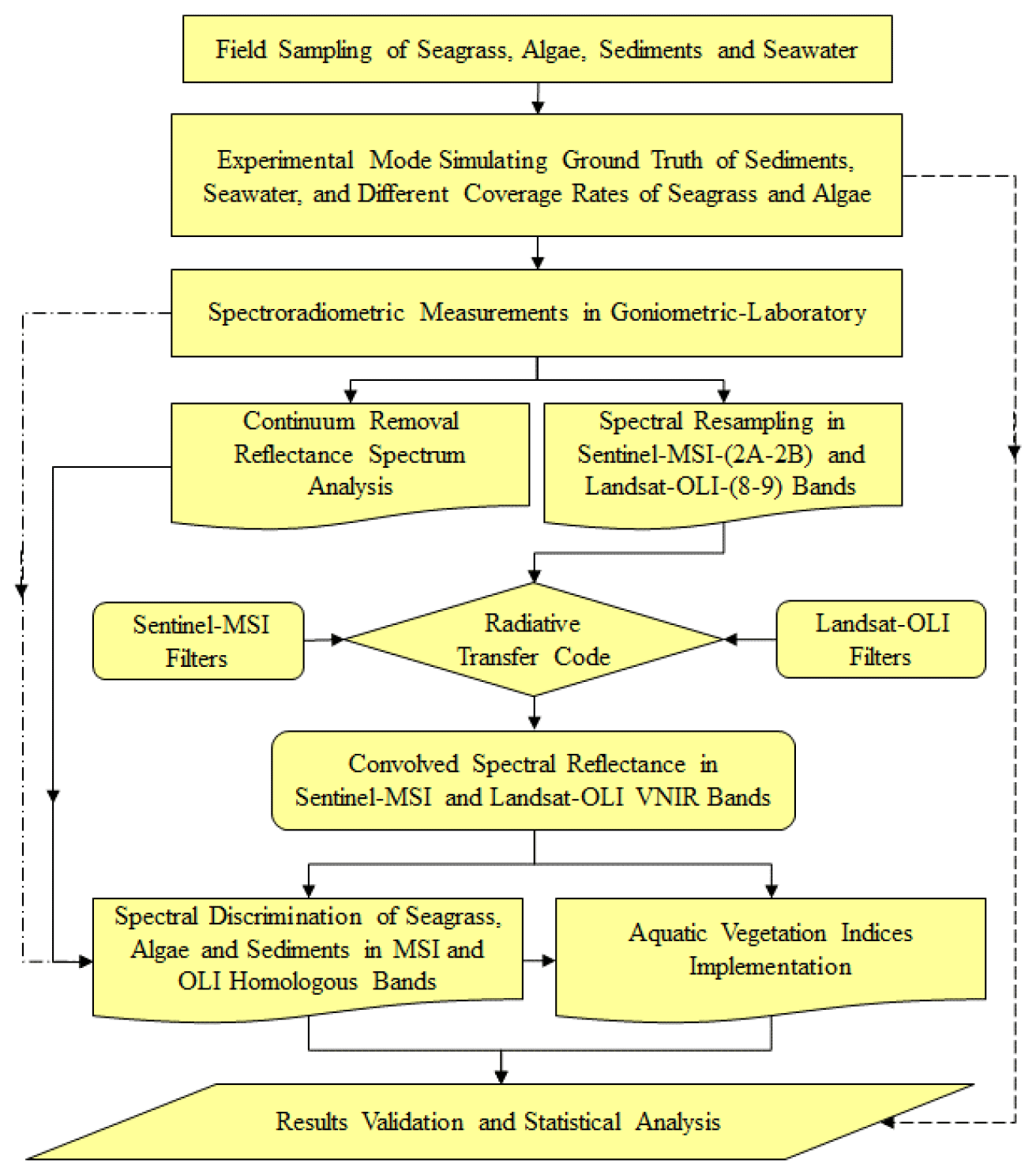
Figure 2 illustrates the followed methodology, which is based on a field survey to collect samples including seawater, sediments, seagrass (Halodule uninervis and Halophila stipulacea), and algae (green and brown) from shallow marine environments at different depths (0.50 to 7 m) off southeast Bahrain Island. To simulate the marine environment, an experimental mode was established in a goniometric laboratory and spectral measurements were performed using an Analytical Spectral Devices (ASD) spectroradiometer over each separate and mixed species at different coverage rates (0 %, 10 %, 30 %, 75 %, and 100 %), as well as simulating the seabed with dark and bright colors. To assess the spectral signatures variability that can be found among each separate or mixed species at varying coverage rates, all measured spectra were analyzed and transformed using continuum-removed reflectance spectral (CRRS) approach (see Sect. 3.4). Then, the spectra were resampled and convolved in the solar-reflective spectral bands of MSI and OLI sensors using the Canadian Modified Simulation of a Satellite Signal in the Solar Spectrum (CAM5S) (Teillet and Santer, 1991) based on Herman radiative transfer code (RTC), and the relative spectral response profiles characterizing the filters of each instrument in the VNIR bands. Afterward, convolved spectra were converted into several WVI integrating the red, green, and blue bands. For comparison and sensor differences quantification, statistical fits were conducted using linear regression analysis (p<0.05) between reflectances in homologous bands and between the examined homologous WVI derived from the two sensors' data considering all samples, i.e., seawater, sediments, seagrass, and algae species (individually and mixed at the considered coverage rates). The coefficient of determination (R²), difference values, and root mean square difference (RMSD) were calculated for reflectances and all versions of investigated WVIs.

Figure 2 Methodology flowchart.

3.1 Study site

The area under investigation in this research is the water boundary of the Kingdom of Bahrain (25^∘32^′ to 26^∘00^′ N, 50^∘20^′ to 50^∘50^′ E), which is a group of islands located in the Arabian Gulf, east of Saudi Arabia and west of Qatar (Fig. 3). The archipelago comprises 33 islands, with a total area of 8269 km²; 9 % of it is a land area (778.4 km²). Along the southeast coast of Bahrain, the continental plateau extends for kilometers with a depth of less than 1 or 2 m. The main island of Bahrain is surrounded by shoal areas named “fashts” where depths do not exceed 10 m (Bannari and Kadhem, 2017). These areas generally support a variety of species of seagrass, algae, coral, and fishes. Moreover, they play an important role in the hydrodynamic regime, which supports diverse biological ecosystems. Figure 3 also illustrates the reclamation and dredging operations that have occurred in the study area over the past three decades where several coastal developmental projects are constructed, and others are in progress. These anthropogenic activities strongly contribute to the degradation and even to the destruction of seagrass species and associated coastal ecosystems.

Figure 3 Study site (Kingdom of Bahrain), with photos illustrating landfill operations (a, b), and satellite images of the south part of Bahrain before (c) and after (d) artificial island construction.

3.2 Field sampling

Seagrass and algae samples were collected on 4 May 2017 from different meadow locations, which are characterized by a depth range from 0.5 to 7 m in the south and southeast waters of Bahrain (Fig. 4a). Some locations were dominated with Halodule uninervis (HU), others were scattered, and others were densely mixed between HU and Halophila stipulacea (HS). HU is the most dominant species (Fig. 4b); it occurs as dense or scattered meadow patches along the shoreline (Erftemeijer and Shail, 2012). This species is like grass with narrow leaves (around 3 mm in width and 25 cm in length), whereas HS (Fig. 4c) has darker green leaves reaching 10 cm in length and it is widely present in the Arabian Gulf. The brown (BA, Fig. 4d) and green (GA, Fig. 4e) algae were accessible near the shores and shallow water in general. In addition to the sediments (Fig. 4f) and pure seawater samples, which were collected separately, samples of each seagrass and algae species were selected and harvested in healthy and fresh conditions from several stations within the study area. Then, they were stored separately in non-translucent plastic bags with seawater and immediately placed in a cooler for transportation from the field to the laboratory. This was done to prevent structural and leaf pigment damages due to the delay between sampling time and spectroradiometric measurements in the goniometric laboratory.

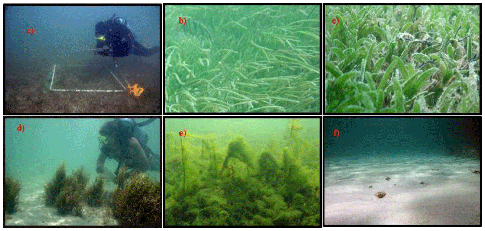
Figure 4 Diver for sampling operation (a) and underwater photos of the considered seagrass and algae species: HU (b), HS (c), BA (d), GA (e), and bright sediments (f).

3.3 Spectroradiometric measurements

Spectroradiometric measurements were acquired in a dark bidirectional reflectance factor (BRDF) goniometric laboratory above each sample separately, then above mixed samples, using an ASD spectroradiometer (ASD, 2015). This instrument is equipped with two detectors, as presented in Fig. 5, operating in the VNIR and shortwave-infrared (SWIR) ranges, between 350 and 2500 nm. It acquires a continuous spectrum with a 1.4 nm sampling interval from 350 to 1000 and 2 nm from 1000 to 2500 nm. The ASD resamples the measurements in 1 nm intervals, which allows the acquisition of 2151 contiguous hyperspectral bands per spectrum. The sensor is characterized by the programming capacity of the integration time, which allows an increase of the SNR and stability. The data were acquired at nadir with a field of view (FOV) of 25^∘ and a solar zenith angle of approximately 5^∘ by averaging 40 measurements. The ASD was installed on a BRDF goniometric system with a height of approximately 65 cm over the target, which makes it possible to observe a surface of ∼ 830 cm². A laser beam was used to locate the center of the ASD FOV. The reflectance factor of each sample was calculated as the ratio of target radiance to the radiance obtained from a calibrated “Spectralon panel” according to the method described by Jackson et al. (1980). Moreover, the corrections were applied for the wavelength dependence and non-Lambertian (i.e., uneven light distribution in all directions) behavior of the panel (Sandmeier et al., 1998; ASD, 2015; Ben-Dor et al., 2015). The measurements were carried out above each collected sample including seawater, sediments, seagrass, and algae species as well as mixed species (seagrass and algae) considering different coverage rates (0 %, 10 %, 30 %, 75 %, and 100 %). Each sample was placed and measured twice in black and bright (yellow) large bowls, considering two sedimentary substrates (dark and bright) underlying the seagrass and algae samples that were submerged by seawater, i.e., simulating the aquatic environment. Since the remote sensing of benthic aquatic vegetation is mostly limited to the VNIR ranges (Fig. 1), only the wavelengths interval between 400 and 1000 nm are considered in our analyses.

Figure 5 Dark goniometric laboratory for ASD measurements.

3.4 Continuum-removed reflectance spectral (CRRS) transformation

Spectral signatures are processed and transformed using numerous approaches to retrieve information about change in absorption features (position, depth, width, and asymmetry) of a particular target over a specific bandwidth between 350 and 2500 nm (Van-Der-Meera, 2004). To emphasize these absorption features, many approaches were proposed including relative absorption-band depth (Crowley et al., 1989), spectral feature fitting technique, and Tricorder and Tetracorder algorithms (Clark et al., 2003). These approaches work on the so-called CRRS approach, thus recognizing that the absorption in a spectrum has a continuum and individual absorption features (Clark et al., 1987; Van-Der-Meera, 2004; Clark et al., 2014). Proposed by Clark and Roush (1984), CRRS transformation and analysis allow the isolation of individual absorption features in the hyperspectral signature of a specific target under investigation, analysis, and comparison. It normalizes the original spectra and helps to compare individual absorption features from a common baseline (Clark et al., 1987). The continuum is a convex hull fit over the top of a spectrum under study using straight-line segments that connect local spectra maxima. The first and last spectral data values are on the hull; therefore, the first and last bands in the output continuum-removed data file are equal to 1.0. In other words, after the continuum is removed, a part of the spectrum without absorption features will have a value of 1, whereas complete absorption would be close to 0, with most absorptions falling somewhere in between. The CRRS approach was used for discriminating and mapping rock mineralogy (Clark et al., 1990; Clark and Swayze, 1995), land vegetation cover (Kokaly et al., 2003; Huang et al., 2004; Manevski et al., 2011), and seagrass and SAV (Barillé et al., 2011; Bargain et al., 2012; Wicaksono et al., 2019; Indayani et al., 2020). In this study, the continuum algorithm implemented in the ENVI image processing system was used (ENVI, 2012).

3.5 Spectral sampling and convolving in MSI and OLI spectral bands

Since 1972, the Landsat scientific collaboration program between NASA and USGS has constituted the continuous record of the Earth's surface reflectivity from space. Indeed, the Landsat satellites series support five decades of a global medium-spatial-resolution data collection, distribution, and archive of the Earth's surfaces (Bannari et al., 2004; Loveland and Dwyer, 2012) to support research, applications, and climate change impacts analysis at the global, regional, and local scales (Roy et al., 2014, 2016; Wulder et al., 2015). Benefiting from the acquired space-engineering experience, from the heritage of Landsat instruments, and the advanced development of technology during the last five decades, the fourth generation of Landsat is composed of two similar sensors with very high spectral and radiometric sensitivities: OLI-1 and OLI-2 (Markham et al., 2016; Li and Chen, 2020). OLI-1, carried aboard Landsat-8, was launched on 11 February 2013, and OLI-2, aboard Landsat-9, was launched on 27 September 2021 (NASA, 2019, 2021). The OLI sensors collect land-surface reflectivity in the VNIR, SWIR, and panchromatic wavelengths with a FOV of 15^∘ covering a swath of 185 km with 16 d time repetition at the Equator. The band passes are narrower to minimize atmospheric absorption features (NASA, 2014), especially the NIR spectral band (0.865 µm). Two new spectral bands have been added: a deep blue visible shorter wavelength (band 1: 0.433–0.453 µm) designed specifically for water resources and coastal zone investigation and a new SWIR band (9: 1.360–1.390 µm) for the detection of cirrus clouds. Moreover, compared to previous TM and ETM+ sensors using only 8 bits, the OLI design results in more sensitive instruments with a significant improvement of the SNR radiometric performance quantized over a 12-bit dynamic range (Level 1 data), and raw data are delivered in 16 bits. The high performance of SNR associated with improved radiometric and spectral resolutions provides a superior dynamic range of radiance by reducing saturation problems and therefore enables better characterization of land and water surface conditions (Knight and Kvaran, 2014), especially with orbit reflective radiometric calibration better than 3 % (Markham et al., 2014; Gascon et al., 2017). Table 1 summarizes the effective bandwidth characteristics of OLI-1 and OLI-2 sensors.

Table 1 The Sentinel-MSI and Landsat-OLI effective bandwidths and characteristics (λ indicates wavelength, SNR is signal to noise ratio, L_ref(λ) indicates reference radiance, E₀(λ) indicates extra-atmospheric irradiance).

Otherwise, the Sentinel-2 mission is the result of close collaboration between the European Space Agency, the European Commission, industry, service providers, and data users. It is composed of two satellites, Sentinel 2A and 2B, that were launched in June 2015 and March 2017, respectively. Both satellites are equipped with identical MSI sensors to provide continuity to the SPOT missions and to improve the Landsat-OLI temporal frequency (Drusch et al., 2012). The synergy between the four sensors (MSI-2A, MSI-2B, OLI-1, and OLI-2) significantly increases the temporal resolution (around 2 d), offering new opportunities for several environmental and natural resource applications, such as the vigor of vegetation cover, emergency management, water quality, seagrass meadows, and climate change impact analysis at local, regional, and global scales. The MSI images the Earth's surface reflectivity with a large FOV (20.6^∘) in 13 spectral bands with several spatial resolutions from 10 to 60 m; four bands with 10 m (blue, green, red, and NIR-1), six bands with 20 m (red edge, NIR-2, and SWIR), and three bands with 60 m (coastal, water vapor, and cirrus). The swath of each scene is 290 km, permitting global coverage of the Earth's surface every 10 d. The MSI radiometric performance is coded in 12 bits, ensuring radiometric calibration accuracy of better than 3 % and an excellent SNR (Markham et al., 2014; Li et al., 2017). Table 1 summarizes the effective bandwidth characteristics of MSI-2A and MSI-2B sensors.

As discussed above, the measured BRDF with the ASD has a 1 nm interval, allowing the acquisition of 2151 contiguous hyperspectral bands per spectrum. However, most multispectral remote sensing instruments measure integrated reflectance over broad bands (Eq. 1). Consequently, the average of 40 spectra measured with the ASD over each sample was resampled and convolved to match the solar-reflective spectral response functions characterizing the optics and electronics of MSI and OLI instruments in the VNIR spectral bands (Fig. 6). In this step, the resampling procedure considers the nominal width of each spectral band (Table 1). Then, the convolution process was executed using the CAM5S transfer radiative code (Teillet and Santer, 1991). This fundamental step simulates the signal received by the considered sensors at the top of the atmosphere from a surface reflecting solar and sky irradiance at sea level, considering the filter of each band (Fig. 6), and assuming ideal atmospheric conditions without scattering or absorption (Zhang and Roy, 2016). Accordingly, the equivalent convolved reflectance (ρ(λ_i, λ_s)i) over each sample was generated at the satellite orbit altitude in homologous VNIR spectral bands of each sensor (Slater, 1980):

$$\begin{array}{}\text{(1)}& \mathit{\rho }{\left({\mathit{\lambda }}_i,{\mathit{\lambda }}_{\mathrm{s}}\right)}_i={\displaystyle \frac{{\int }_{{\mathit{\lambda }}_i}^{{\mathit{\lambda }}_{\mathrm{s}}}R\left(\mathit{\lambda }\right)\cdot S{\left(\mathit{\lambda }\right)}_i\cdot \mathrm{d}\left(\mathit{\lambda }\right)}{{\int }_{{\mathit{\lambda }}_i}^{{\mathit{\lambda }}_{\mathrm{s}}}S{\left(\mathit{\lambda }\right)}_i\cdot \mathrm{d}\left(\mathit{\lambda }\right)}},\end{array}$$

where ρ(λ_i, λ_s)i is the equivalent convolved reflectance of the band “i” of each sensor, λ_i to λ_s are the spectral wavelength ranges of the band “i” of each sensor, R(λ) is the corresponding reflectance at wavelength “λ” measured by the ASD, and S(λ)_i is the corresponding spectral responsivity value of the spectral response function of the band “i” of each sensor (Fig. 6). It is important to note that the MSI-NIR-2 broadband (band 8: 785–900 nm) is not considered in this study because it is not a real homologous band of OLI-NIR, and it has a greatest reflective band difference with the OLI-NIR (851–879 nm). The OLI-NIR spectral response function intersects with only 20 % of the MSI-NIR-2 response function. Moreover, the MSI red-edge bands were not considered as they are not acquired by the OLI sensor.

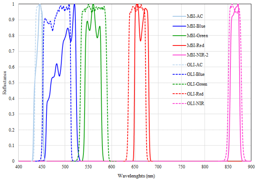
Figure 6 Sentinel-MSI and Landsat-OLI relative spectral response profiles characterizing the filters of each spectral band in the VNIR.

3.6 Data processing

In addition to remote sensing sensor technologies' improvement and innovation, a variety of processing methods has been applied for spectral data for mapping and monitoring seagrass and habitats in shallow coastal waters. They were applied to highlight the seagrass and algae species' composition, leaf area index estimation, percentage cover mapping, etc. They include matched filtering approach (Li et al., 2012), object-based image analysis (Roelfsema et al., 2014), adaptive coherence estimator and constrained energy minimization (Li et al., 2012), artificial neural network model (Perez et al., 2020), linear spectral mixture analysis (Uhrin and Townsend, 2016; Chen et al., 2016), spectral angle mapper (Peneva et al., 2008; Li et al., 2012; Marcello et al., 2018; Wicaksono et al., 2019), classification tree analysis (Wicaksono et al., 2019), random forests (Bayyana et al., 2020), support vector machines (Marcello et al., 2018; Bakirman and Gumusay, 2020; Perez et al., 2020; Bayyana et al., 2020), and machine learning regression (Traganos, 2020; Bakirman and Gumusay, 2020). Undeniably, these sophisticated and complicated methods require extensive training information and field endmember measurements. However, the simplicity of empirical and semi-empirical methods based on vegetation indices are easier to transfer between sensors and can be used as a robust alternative compared to the complex processing methods, because these methods are based on the knowledge of spectral absorption features that characterize specifically the target under investigation. Moreover, these methods have the advantage of being reproducible, easily transferable, and applicable in other geographic regions. Each method has advantages and limitations, especially in shallow water. In this study, after the spectral analysis and CRRS transformation, the capabilities and comparison of the VNIR homologous spectral bands of MSI and OLI sensors were investigated for seawater, sediments, seagrass, algae, and mixed species discrimination at different coverage rates. Then, although the literature refers to more than 50 vegetation indices for land vegetation cover monitoring and characterization (Bannari et al., 1995), only the most popular indices that have been used for seagrass and SAV in different marine environments around the world were retained in this study. After spectral data pre-processing, sampling, and convolving, the TGI, VARI, and Diff(G-B) indices were implemented and tested respecting their original equations, while the NDVI, SAVI, EVI, TDVI, NDWI, and DVI indices were calculated in three versions by integrating the red, blue, and green bands. The equations of the considered indices are as follows:

$$\begin{array}{}\text{(2)}& {\displaystyle }\begin{array}{rl}\mathrm{NDVI}=& \left({\mathit{\rho }}_{\mathrm{NIR}}-{\mathit{\rho }}_{\mathrm{Red}}\right)/\left({\mathit{\rho }}_{\mathrm{NIR}}+{\mathit{\rho }}_{\mathrm{Red}}\right)\\ & \left(\text{Rouse et al., 1974}\right)\end{array}\text{(3)}& {\displaystyle }\begin{array}{rl}\mathrm{SAVI}=& \mathrm{1.5}\cdot \left({\mathit{\rho }}_{\mathrm{NIR}}-{\mathit{\rho }}_{\mathrm{Red}}\right)/\left({\mathit{\rho }}_{\mathrm{NIR}}+{\mathit{\rho }}_{\mathrm{Red}}+\mathrm{0.5}\right)\\ & \left(\text{Huete, 1988}\right)\end{array}\text{(4)}& {\displaystyle }\begin{array}{rl}\mathrm{TDVI}=& \mathrm{1.5}\cdot \left({\mathit{\rho }}_{\mathrm{NIR}}-{\mathit{\rho }}_{\mathrm{Red}}\right)/\left(\sqrt{\left({\mathit{\rho }}_{\mathrm{NIR}}^{\mathrm{2}}+{\mathit{\rho }}_{\mathrm{Red}}+\mathrm{0.5}\right)}\right)\\ & \left(\text{Bannari et al., 2002}\right)\end{array}\text{(5)}& {\displaystyle }\begin{array}{rl}\mathrm{NDWI}=& \left({\mathit{\rho }}_{\mathrm{Green}}-{\mathit{\rho }}_{\mathrm{NIR}}\right)/\left({\mathit{\rho }}_{\mathrm{Green}}+{\mathit{\rho }}_{\mathrm{NIR}}\right)\\ & \left(\text{McFeeters, 1996}\right)\end{array}\text{(6)}& {\displaystyle }\begin{array}{rl}\mathrm{EVI}=& \mathrm{2.5}\cdot \left({\mathit{\rho }}_{\mathrm{NIR}}-{\mathit{\rho }}_{\mathrm{Red}}\right)/\\ & \left({\mathit{\rho }}_{\mathrm{NIR}}+\mathrm{6}\cdot {\mathit{\rho }}_{\mathrm{Red}}-\mathrm{7.5}\cdot {\mathit{\rho }}_{\mathrm{Blue}}+\mathrm{1}\right)\\ & \left(\text{Huete et al., 2002}\right)\end{array}\text{(7)}& {\displaystyle }\begin{array}{rl}\mathrm{DVI}=& {\mathit{\rho }}_{\mathrm{NIR}}-{\mathit{\rho }}_{\mathrm{Red}}\\ & \left(\text{Richardson and Wiegand, 1977}\right)\end{array}\text{(8)}& {\displaystyle }\begin{array}{rl}\mathrm{VARI}=& \left({\mathit{\rho }}_{\mathrm{Green}}-{\mathit{\rho }}_{\mathrm{Red}}\right)/\left({\mathit{\rho }}_{\mathrm{Green}}+{\mathit{\rho }}_{\mathrm{Red}}-{\mathit{\rho }}_{\mathrm{Blue}}\right)\\ & \left(\text{Gitelson et al., 2002a}\right)\end{array}\text{(9)}& {\displaystyle }\begin{array}{rl}\mathrm{TGI}=& {\mathit{\rho }}_{\mathrm{Green}}-\mathrm{0.39}\cdot {\mathit{\rho }}_{\mathrm{Red}}-\mathrm{0.61}\cdot {\mathit{\rho }}_{\mathrm{Blue}}\\ & \left(\text{Hunt et al., 2013}\right)\end{array}\text{(10)}& {\displaystyle }\begin{array}{rl}-\text{Diff(G-B)}=& {\mathit{\rho }}_{\mathrm{Blue}}-{\mathit{\rho }}_{\mathrm{Green}}\\ & \left(\text{Mumby et al., 1997}\right)\end{array}\end{array}$$

The wavelength ranges of the used VNIR bands for Sentinel-MSI and Landsat-OLI are summarize in Table 1.

3.7 Statistical analyses

As discussed previously, the respective MSI and OLI spectral response profiles characterizing the filters of each spectral band differ somewhat (Fig. 6). To examine the impact of this difference, statistical analyses were computed using Statistica software. The relationships between the product values (reflectances and WVIs) derived from MSI against those obtained from OLI were analyzed between homologous bands using a linear regression model (p<0.05). As well, the R² was used to evaluate the strength of this linear relationship. For this process, the resampled and convolved spectra of all samples' reflectance data were used, and the homologous values in VNIR bands of MSI and OLI were compared using the 1:1 line. Ideally, these independent variable values should have a correspondence of 1:1. Additionally, the root mean square difference (RMSD) between both sensors was derived (Willmott, 1982; Zhang et al., 2018):

$$\begin{array}{}\text{(11)}& \mathrm{RMSD}=\sqrt{{\displaystyle \frac{{\sum }_i^n{\left(v_i^{\mathrm{OLI}}-v_i^{\mathrm{MSI}}\right)}^{\mathrm{2}}}{n}}},\end{array}$$

where RMSD is between corresponding Landsat-OLI and Sentinel-MSI variable values (reflectances and WVIs), “v_i” is the variable under analysis, and “i” is its index (i=1 to n).

4 Results analysis

4.1 Spectral and CRRS analyses

Spectral signatures of seagrass and algae species are measured separately and mixed in black and yellow large bowls using two sedimentary substrates (dark and bright). They are presented separately for the examined coverage rates, namely 10 %, 30 %, 75 %, and 100 % (Fig. 7a–d). Overall, the reflectance signatures of seagrass and algae samples are similar to those of healthy vegetation canopy. These reflectance signatures exhibit slight absorption features near 450 nm and others stronger between 650 and 700 nm with a minimum at 670 nm caused by the chlorophyll, as well as a significant reflection between 520 and 600 nm due to carotenoid pigments and high reflectance in the NIR attributed to internal tissue structure (700 to 900 nm). Differently from land vegetation, the red edge is not well developed (very weak) particularly for non-dense seagrass and algae due to high red and NIR absorption by water molecules as shown in Fig. 1. Generally, absorption or reflection of pigmentations between species occurs in different wavelengths but the strength of absorption gradually increases in the red as the coverage rate increases.

For scattered and low coverage (∼ 10 %), the shapes of all spectra are similar, without the possibility to identify specific absorption features or to separate among species according to their spectra in the visible domain (Fig. 7a). The highest reflectance values vary between 10 % and 15 % across NIR wavelengths, and a difference reflectance (Δρ_NIR) around 5 %, while in the visible all the reflectance values are below 5 % with Δρ_visible are also <5 %. For this low and sparse cover, it is observed that the reflectance is influenced by spectral properties of the underlying sediments, fragments of vegetation, light shading, etc., thus contributing to the confusion between spectral signatures. Definitely, under such conditions, it is a challenge to distinguish between seagrass and/or algae species based only on their spectral signatures, whereas the measurements acquired over somewhat denser coverage rates (∼ 30 %) show analogous spectral behavior and patterns with overlap among spectra in visible wavelengths (400 to 700 nm), but a slight separability between species is relatively apparent in NIR (Fig. 7b).

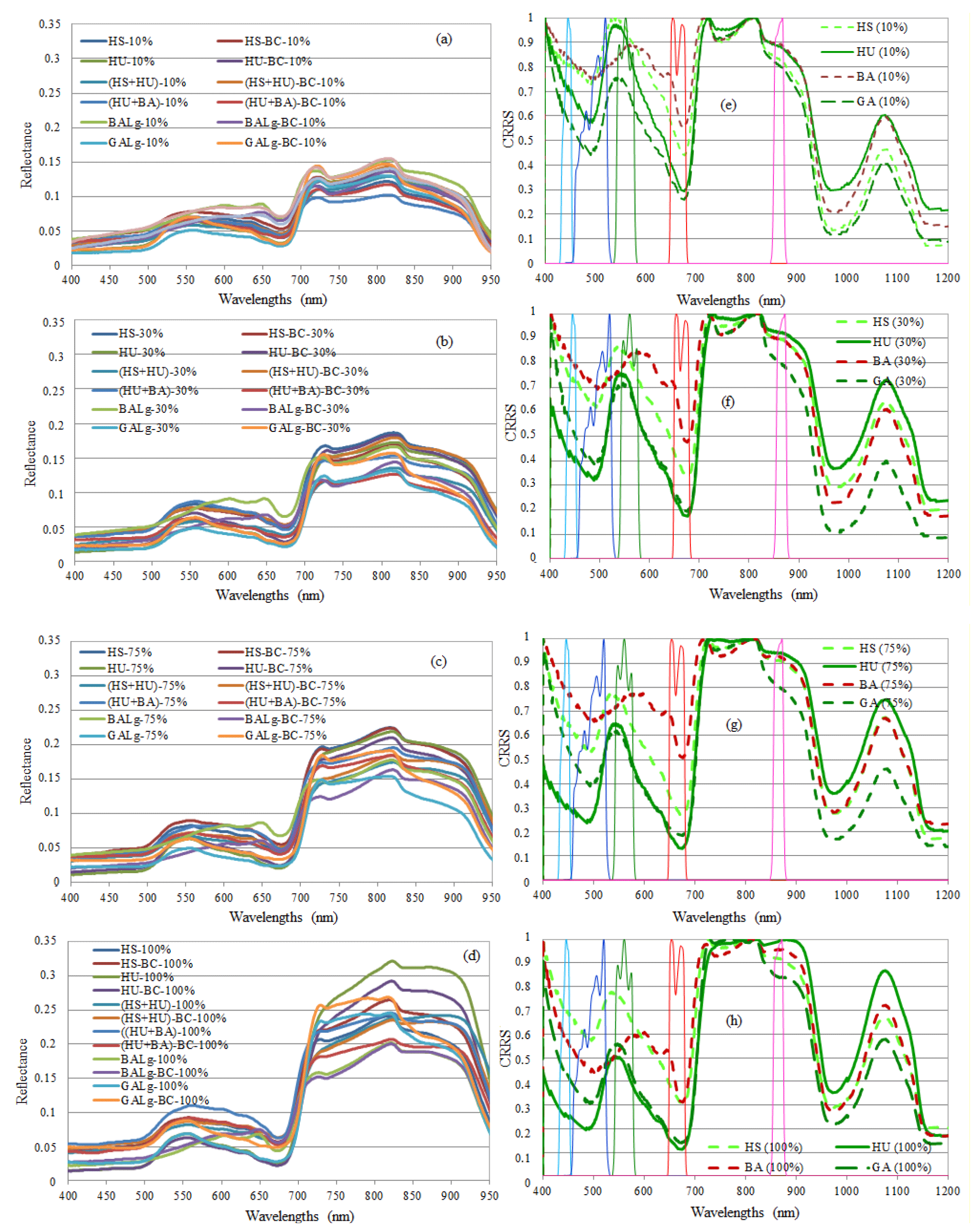
Figure 7 Spectral signatures of seagrass and algae samples at different coverage rates (a: 10 %, b: 30 %, c: 75 %, and d: 100 %) and their CRRS transformations with the filters of Sentinel-MSI VNIR bands presented in Fig. 6.

Furthermore, unlike scattered or less dense cover (≤ 30 %), the analysis of the dense and very dense coverage rates (75 % and 100 %) showed that the optical properties (darkness or brightness) of the underlying substrate do not have a significant effect on the measured spectra. For these coverage ranges, the clear and normal behavior of vegetation cover spectra are observed. The absorption feature is weak in the blue (450–480 nm) but more accentuated in red (670 nm), the reflection peak is more highlighted in green (550 nm), and the reflectance values increase notably and gradually in NIR with the increase of the coverage rate. Although the seagrass has a distinct spectral response compared to the algae, especially in the green and NIR regions of the spectrum, significant spectral differences are noted for the HU with the highest reflectance, followed by GA, HS, and BA. This order is probably controlled by the leaf structures that are specific for each type of seagrass or algae. The reflectance values in the visible are controlled by the absorption of chlorophyll pigmentations in blue and red wavelengths and by the carotenoid pigmentations in the green band. In addition, compared to HS and BA spectra, HU and GA showed relatively strong absorption by chlorophyll in red wavelengths. This difference is due to the nature of chlorophyll in each species. Indeed, brown algae contain accessory pigments “fucoxanthin” and chlorophyll “c” (Johnsen and Sakshaug, 2007), while seagrasses are flowering plants, and their leaves contain chlorophyll “b” (Cummings and Zimmerman, 2003). It is observed also that the BA carotenoid pigments (fucoxanthin) are characterized by spectral features at 630 and 650 nm that are not present in the spectra of HS, HU, and GA (Fig. 7). However, despite all these spectral characteristics the difference in reflectance values among all species (individual and mixed) is ≤ 6 % in the visible and ≤ 13 % in NIR for a very dense cover (100 %). Therefore, these results suggest that it is probably possible for the blue, green, and NIR wavelengths to discriminate among the considered seagrass and algae species if they are homogeneous with high or very high densities.

Otherwise, the CRRS transformations are presented in Fig. 7e–h with Sentinel-MSI relative spectral response profiles characterizing the filters of VNIR bands. The lower CRRS values indicate the greatest potential spectral separability, which means the identification of the appropriate wavelengths to discriminate among the considered classes of investigated species. As shown in Fig. 7e–h, the CRRS significantly enhances the spectral separability among the seagrass and algae classes, especially in the visible bands. Two main absorption features are highlighted in the blue (485–498 nm) and red (∼ 670 nm) regardless the species. In the green, one major reflection peak is observed around 544 nm for HU and GA, one around 530 nm for HS, and three peaks are well distinguished for BA at 578, 595, and 640 nm (Fig. 7h). These differentiation features become clearer as the coverage rates increase especially in blue and NIR wavelengths. For a low coverage rate (∼ 10 %), the strongest absorption depth is that of GA (0.46), followed by HU (0.58), HS (0.74), and BA (0.78) in the blue (Fig. 7e). Meanwhile in the red, CRRS pointed out that regardless of the coverage rate, a strong similarity is observed between HU and GA due to their high content of chlorophyll pigmentation with a depth of absorption around 0.29, followed by HS and BA that are characterized by less absorption depth (∼ 0.50). In these two waveband domains (blue and red), the absorption features become deeper with increasing coverage density. Likewise, when the cover rate of all species becomes denser (100 %), similar absorption characteristics are exhibited in the red band between HU and GA species, as well as between HS and BA (Fig. 7h). Meanwhile in the blue and NIR wavelengths, the CRRS highlights the distinction and differentiation between species. On the other hand, as the coverage increases from 10 % to 100 %, the reflection peak in the green waveband becomes less pronounced due to the high content of carotenoid pigment; also a strong similarity is observed between HU and GA. Moreover, the curves of CRRS of the mixed species occupy an intermediate position of absorption features between the homogeneous samples, and therefore the differentiation between absorption characteristics becomes very slight. Accordingly, the discrimination between pure and mixed species becomes very difficult or even impossible. Overall, spectral and CRRS analyses highlighted the importance of the blue, green, and NIR wavelengths for seagrass and algae detection and probable discrimination based on hyperspectral measurements. These results corroborate the physical concept presented in Fig. 1 that the blue and green electromagnetic radiation penetrates a deeper vertical column of water, while despite its limited penetration, the NIR shows a certain sensitivity to the biomass density and its spatial distribution.

4.2 Resampling and convolving in OLI and MSI bands

Figure 8 illustrates the scatterplots between the resampled and convolved reflectance values in the VNIR homologous bands of the MSI and OLI sensors. Simulated at the top of the atmosphere using all considered samples (seawater, sediments, seagrass, algae, and mixed species of both seagrass and algae at varied coverage rates), they allow the analysis of the difference in reflectance values (Δρ) and RMSD due exclusively to dissimilarities in spectral response function between homologous bands. These scatterplots reveal a near-perfect fit with 1:1 line expressing an excellent coefficient of determination (R² of 0.999) between homologous bands with the slopes and intercepts very close to unity and zero, respectively. Thus, the derived Δρ values are null for VNIR homologous bands for seawater and are insignificant for dark and bright substrate sediments in all bands (i.e., 0.009 for green and 0.002 for the coastal, blue, red, and NIR bands). Meanwhile, for seagrass and algae (HS, HU, GA, and BA), Δρ varies between 0.003 and 0.02 regardless of the coverage rate or the considered spectral band. Moreover, the achieved overall RMSD in reflectance between MSI and OLI homologous bands considering all samples is insignificant (≤ 0.0015) for blue, green, and red bands, and null for coastal and NIR bands. It is also observed that all the bands are insensitive to the variation of the colors of the bowls and the sedimentary substrate optical properties. These results pointed out that MSI and OLI sensors are spectrally similar and can be used jointly for high temporal frequency to monitor seagrass and algae dynamics in time and space. Therefore, due to this near-perfect spectral similarity between these instruments, our analysis in the following sections will focus only on the MSI sensor.

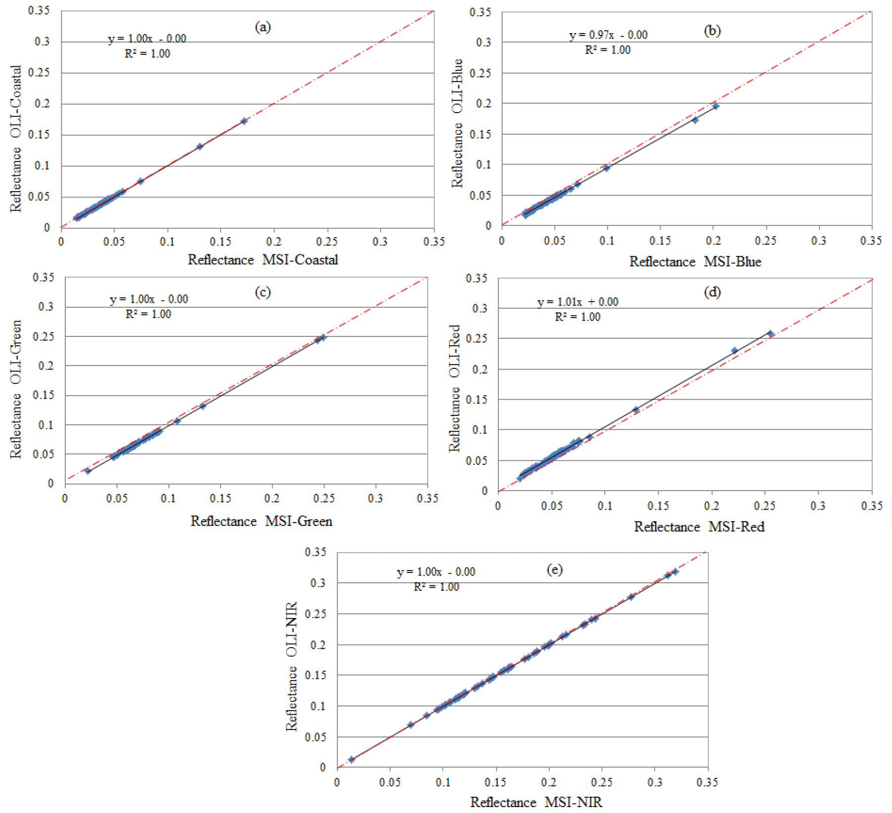
Figure 8 Scatterplots of reflectances sampled and convolved in MSI and OLI homologous spectral bands.

Figure 9 illustrates the reflectances of seagrass, algae, and seawater resampled and convolved in VNIR bands of MSI or OLI sensors considering each species separately and all species at different coverage rates. Compared to the measured hyperspectral signatures (Fig. 7), these broadband spectra are more generalized and less precise because these spectra lost the specific and unique absorption features of seagrass and/or algae species caused by pigmentations as discussed above. However, such broadband spectra retain the same spectral pattern as the original spectra. Regardless of the species, the graphics summarized in Fig. 9 exhibit a similar shape and pattern but with a slight difference in reflectance values between species in the visible bands. If we consider the species separately (HS, HU, GA, and BA) in different coverage rates (10 %, 25 %, 75 %, and 100 %), the reflectance difference values (Δρ) are ≤ 0.02 and insignificant (Δρ≤ 0.002) for pure seawater and sediments in all VNIR bands. Hence, these species are not spectrally distinguishable particularly in the visible whatever the coverage. Meanwhile, if we consider all samples (seagrass, algae, and mixed) in all coverage rates (Fig. 9e), the Δρ values are equal to 0.03 in coastal and blue bands, 0.05 in green, 0.035 in red, and 0.21 in NIR. Except for the NIR, the calculated Δρ values in the visible are approximately identical to the accuracies achieved from radiometric calibration and atmospheric corrections. Therefore, relying on the multispectral bandwidth of OLI and MSI sensors, it is difficult or even impossible to differentiate or to map seagrass and algae individually at the species level. Accordingly, SAV classes' discrimination and mapping will be discussed.

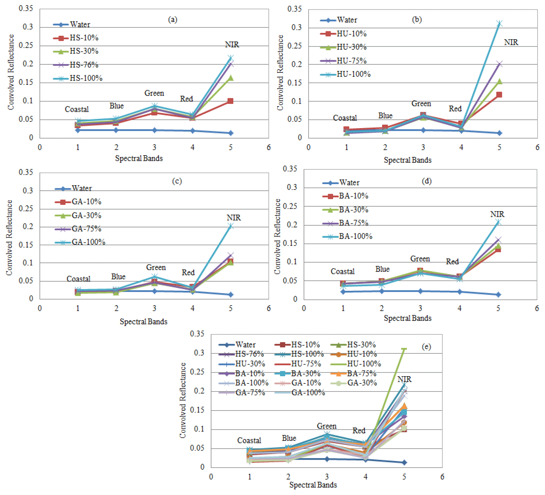
Figure 9 Seagrass, algae, and seawater reflectances resampled and convolved in VNIR bands of Sentinel-MSI (or Landsat-OLI): HS (a), HU (b), GA (c), BA (d), and all samples (e).

4.3 Vegetation indices' analysis

In this third part, the NDVI, SAVI, EVI, TDVI, NDWI, and DVI indices were implemented and analyzed in three versions each by integrating the red, blue, and green bands, while the indices TGI, VARI, and Diff(G-B) were calculated and tested respecting their original equations. In total, 21 combinations of indices were calculated for each sensor. The statistical analyses (p<0.05) focus on the similarity or dissimilarity between MSI and OLI homologous indices and their potential for seagrass and algae discrimination. Except for the TGI and VARI indices, the results revealed an excellent linear relationship (R² of 0.999) between MSI and OLI products regardless of the compared index and the integrated spectral bands (red, green, and blue). Overall, the scatterplots presented in Fig. 10 depict a very good fit to the 1:1 line with the slopes and intercepts very close to unity and zero, respectively. However, despite its near-perfect linearity and insignificant RMSD between MSI and OLI values (0.001), the TGI show a very weak and limited spatial variability with a range between 0.0 for pure seawater and 0.05 for a very dense coverage (100 %) of seagrass or algae (Fig. 10e). This range cannot allow the differentiation among the marine environment classes, because this index was not developed for biomass sensing but was designed for crop nitrogen requirement detection. Likewise, although the scatterplot of VARI shows an excellent coefficient of determination (R² of 0.99), estimates of this index with the MSI sensor exceed those from OLI, resulting in the data not fitting the 1:1 line very well (Fig. 10f). Moreover, the difference values of VARI derived from MSI and OLI data vary between 0.0 and 0.14 depending on the sample species and its coverage rate, with an overall RMSD of 0.03. This result can be explained by the fact that the VARI uses only the visible ranges of the spectrum and does not consider the NIR band, which is the most informative about the biomass density. In addition, it was developed particularly for very dense (100 %) wheat crops; moreover, it was designed principally for coarse data acquired by the SeaWiFS, MODIS, MISR, and MERIS sensors. According to Gitelson et al. (2002b), many factors potentially decrease the accuracy of the VARI (e.g., vegetation cover species, canopy architecture, and Sun illumination geometry). For wheat and corn species, this index yielded RMSE of around 10 % (Gitelson et al., 2002a). Therefore, the weaknesses raised for these two indices (TGI and VARI) are not caused by the impact due exclusively to the dissimilarities in spectral response function between homologous bands of MSI and OLI sensors but are due to their mathematical concepts that are intended for a single and specific application.

Figure 10 Scatterplots of homologous WVI derived from MSI and OLI simulated data.

Furthermore, the scatterplots presented in Fig. 10a–d show examples of certain indices including NDWI, WAVI, water enhanced vegetation index (WEVI), and water transformed difference vegetation index (WTDVI). Overall, the indices fit the 1:1 line very well with R² of 0.99, slopes very close to unity, and intercepts to zero. The indices show that the derived WVI from MSI and OLI data gives similar estimates of seagrass and algae species in a shallow marine environment. Considering all investigated samples in this study, the interval difference values between homologous indices vary between 0.0 and 0.01 for all versions of WTDVI, WAVI, WDVI, and Diff(G-B), while they vary between 0.0 and 0.04 for NDWI, WEVI, and NDWI. These difference values are satisfactory and remain equal to or less than the combined inaccuracies of atmospheric corrections and sensor radiometric calibration. Moreover, the achieved RMSD values between MSI and OLI homologous indices are insignificant (RMSD ≤ 0.01) for all indices (Table 2) regardless of the integrated spectral band. These analyses pointed out that MSI and OLI sensors can be combined for high temporal frequency to monitor the dynamic of biophysical products in time and space in a shallow marine environment.

Table 2 R² (p<0.05) between vegetation indices integrating red, blue, and green bands and the reflectances in NIR for all considered samples, and the RMSD between indices derived from MSI and OLI sensor data.

^*  indicates the RMSD between indices derived from MSI and OLI simulated data. The bold type highlights the significant R² values.

Figure 11 summarizes the linear regressions (p<0.05) between the best indices and the reflectances in NIR considering all samples, i.e., seawater, sediments, seagrass, algae, and mixed species classes with different coverage rates (10 %, 30 %, 75 %, and 100 %). The computed indices (NDVI, SAVI, EVI, TDVI, NDWI, and DVI) with the blue, green, and red bands are the most relevant for SAV differentiation and mapping. Firstly, it is observed that the indices NDVI and NDWI provided similar results with opposite signs, i.e., symmetrically opposed concerning the x axis. Indeed, whatever the integrated band, the NDWI results are always symmetrical compared to those of NDVI but with negative values. However, such results are not showing the truth because negative values are automatically reset to zero by the image processing system, and therefore it is probable that the results will be inaccurate. Furthermore, when the red and blue bands are implemented in the NDVI equation, insignificant fits (R² of 0.40) were achieved, whereas improved results are obtained with the integration of the green band (R² of 0.63) and the index is named the normalized difference water vegetation index (NDWVI). Analogous results are obtained by Diff(G-B) and VARI indices with R² of 0.63 (Table 2) when all samples are considered. Luckily, the statistical fits of these three indices (NDWVI, Diff(G-B), and VARI) become significantly improved when unique species are considered, such as only seagrass or only algae (R² of 0.85), whereas, in addition to its weakness and limited sensitivity to the spatial variability of seagrass and algae, the TGI was irrelevant for SAV discrimination, yielding a very low fit (R² of 0.20) whatever the considered species.

Figure 11 Linear regressions (p<0.05) between WVI and reflectance in NIR considering all samples, and integrating the red, green, and blue bands.

As discussed previously, when integrating the blue and green bands, the WDVI, WAVI, WEVI, and WTDVI indices outperformed all examined indices regardless of the species (seagrass, algae, or mixed), yielding a very significant coefficient of determination for mixed species (0.89 ≤ R²≤ 0.96) (Fig. 11a–d and Table 2). Calculated with blue, green, or red bands, the DVI (denoted as WDVI) discriminated among SAV classes significantly (R²≤0.92), but it underestimates the SAV as shown in Fig. 10d. However, WAVI, WEVI, and WTDVI offer similar trends regardless the considered species (R²≤0.92 for mixed or seagrass only, and R² of 0.82 for algae only). Overall, instead of the red band, the integration of blue and green bands in vegetation indices increases their discriminating power for SAV (Table 2). These results corroborate the spectral analysis and the CRRS transformations; the blue and green electromagnetic radiation penetrates deeper through the water allowing more details and information about marine vegetation discrimination. This finding is consistent with Wicaksono and Hafizt (2013) and Villa et al. (2014), where the blue band better separates and maps aquatic vegetation features over some lake ecosystems in Italy. However, the summarized R² in Table 2 shows that the indices WAVI, WEVI, and WTDVI provided very close results when integrating the blue or green bands. Nevertheless, the scatterplots in Fig. 11a, b, and c illustrate that when the green band is considered instead of the blue, the majority of sampled points are located closer to 1:1 line, especially when the coverage rate becomes denser. This can be explained by the fact that despite the power of blue wavelengths to penetrate deeper into the water, this band also leads to an overestimation of indices' values due to its higher scattering (Fig. 11), mainly in turbid environments.

5 Discussion

Seagrass and algae species showed similar spectral signature curves but with subtle differences between species. In general, some relevant wavelengths are observed for the characterization of the considered species of seagrass and algae including those at or near 450, 500, 520, 550, 600, 620, 640, 670, and 700 nm. They are related to the absorption features and reflection peaks due to photosynthetic pigmentations of HU, HS, GA, and BA. Spectral and CRRS analyses highlighted the importance of the blue, green, and NIR wavelengths for probable differentiation between the considered seagrass and algae types. However, the magnitude of the Δρ values among species is an indicator of the strength of the absorption feature depths and therefore of their discriminating power between species. For instance, the highest Δρ value among all considered samples (seagrass, algae, and mix of both) is ≤ 5 % across the visible wavelengths and around 10 % to 15 % in NIR. Likewise, the CRRS transformations of all spectra of homogeneous and mixed samples show that the absorption characteristics become all very similar, and thus the discrimination between pure and mixed species becomes difficult or even impossible. These results are in agreement with other findings that have been conducted in many geographic locations worldwide and have considered many seagrass and algae types. Considering nine tropical species of seagrass, Wicaksono et al. (2019) showed that even hyperspectral data will not improve discrimination between seagrass and algae at the species level in pixels or subpixels due to the subtle difference in absorption features among them. In addition, Phinn et al. (2008) confirmed that the hyperspectral data are unable to map seagrass biomass at the species level in shallow waters of Moreton Bay in Australia. Using field and laboratory hyperspectral measurements over several seagrass species on the west coast of Florida, Pu et al. (2012) reported also that the VNIR wavelengths have relatively low accuracies to discriminate among seagrass community composition.

Otherwise, the resampled and convolved spectra in VNIR bands of MSI and OLI sensors are similar in all cases, considering each species separately or the totality of samples at different coverage rates. These spectra are more generalized and less precise due to the loss of absorption features caused by pigmentations. Hence, regardless of the coverage rates, if uniform and homogeneous species are considered, the Δρ is ≤ 0.02 in the visible and ≤ 0.22 in NIR. Meanwhile, if all mixed samples and species are considered at the investigated coverage rates, Δρ is ≤ 0.05 in visible bands and remains stable (Δρ≤ 0.22) in NIR. These very small values do not allow spectral distinction among species, particularly in the visible wavebands. Therefore, based on the multispectral bandwidth of OLI and MSI sensors, it is difficult to differentiate seagrass and algae individually at the species level. Indeed, it is important to remember that these simulations were conducted in a goniometric laboratory using close-range measurement protocol and supervising rigorously all measured samples, i.e., homogeneous or mixed. Moreover, in this controlled environment, the atmospheric scattering and absorption are absent; errors related to the sensor radiometric calibration are also absent, with no wave variation, no residual clouds contamination, no Sun glint (specular effects), no variability in water depth, and no BRDF impact. However, the results obtained are not entirely conclusive and do not provide a clear and satisfactory distinction among the spectral signatures of the investigated species. The difference among spectral signatures is surely reduced in the real world when seagrasses and algae are embedded in sediments and overlaid by the water column and constituents including phytoplankton, suspended organic and inorganic matter, variability in water depth, and remote sensing problems (internal and external). Additionally, the acquired images with Sentinel-MSI (2A and 2B) and Landsat-OLI (8 and 9) sensors are coded radiometrically in 12 and 16 bits, respectively. These images cover dissimilar pixels surfaces of 100 m² for MSI and 900 m² for OLI, where SAV information can be easily mixed within pixels. Besides, the FOV of these instruments are different, OLI's FOV is 15^∘ covering a swath of 185 km, while the MSI is characterized by a large FOV of 20.6^∘ covering a swath of 290 km, which requires the adjustments to reduce differences caused by BRDF effects (acquisition and Sun illumination geometries). Data quality may also change due to the sensor's radiometric performance, SNR, and atmospheric interferences (diffusion and absorption). Despite corrections of all these anomalies before the information extraction, biases still occur generated by error propagation, which affect the recorded signal at the sensor level and, therefore, the precision of discrimination between seagrass and algae at the species level. For instance, if we consider the published RMSE regarding each source of error separately, the calculated total RMSE based on error propagation theory (Eq. 12) will be approximately 0.08 to 0.10 (reflectance unit). Therefore, this total RMSE is greater than the achieved difference between reflectance values (Δρ≤ 0.05), especially in the visible bands. Accordingly, it is impossible to differentiate between seagrass and algae at the species level. Likewise, this total RMSE is solely due to the limitations of remote sensing methods, but it can also be amplified by environmental aspects of seagrass habitat, as discussed above and reported by Wicaksono and Hafizt (2013).

$$\begin{array}{}\text{(12)}& \begin{array}{rl}{\mathrm{RMSE}}_{\mathrm{Total}}& =[{\left({\mathit{\sigma }}_{\text{Sensor drift}}\right)}^{\mathrm{2}}+{\left({\mathit{\sigma }}_{\mathrm{Atmosphere}}\right)}^{\mathrm{2}}\\ & +{\left({\mathit{\sigma }}_{\text{Sun glint}}\right)}^{\mathrm{2}}+{\left({\mathit{\sigma }}_{\mathrm{BRDF}}\right)}^{\mathrm{2}}\\ & +{\left({\mathit{\sigma }}_{\text{Water column}}\right)}^{\mathrm{2}}{]}^{\mathrm{0.5}},\end{array}\end{array}$$

where σ_{sensor drift}: sensor radiometric calibration accuracy, ± 0.03 (Markhman et al., 2014, 2016), σ_atmosphere: atmospheric corrections accuracy, mostly around ± 0.03 to ± 0.05 in the visible bands (Vermote et al., 2016), σ_{Sun glint}: Sun glint correction accuracy, ± 0.05 (Zorrilla et al., 2019), σ_BRDF: accuracy of BRDF correction for MSI, ± 0.05 to ± 0.08 (Roy et al., 2017), and σ_{water column}: accuracy of water column correction, ± 0.04 (Zoffoli et al., 2014).

The results of this research accomplished in the Arabian Gulf species based on spectroradiometric measurements are consistent with other research carried out in many geographical regions worldwide. Barillé et al. (2009) showed the degradation of spectral features when resampled into SPOT-HRV visible bands, and therefore seagrass species could no longer be discriminated in these wavelengths. This statement is also in agreement with Wicaksono et al. (2017), who reported that resampled spectra in MSI and OLI bands do not have sufficient spectral information for seagrass species discrimination for accurate classification. Using MSI and OLI data with, respectively, 10 and 30 m pixel sizes (i.e., each OLI pixel is represented by 9 MSI pixels), Lyons et al. (2011) reported relatively accurate discrimination between seagrass meadow spots that are very large with homogenous composition and distinct boundaries between species. Meanwhile, the differentiation becomes impossible when the analyzed spots are composed of diverse species and scattered without clear boundaries.

Furthermore, to analyze the impact of differences in reflectance exclusively due to dissimilarities in spectral response function between homologous spectral bands, the scatterplots between MSI and OLI simulated surface reflectance values at the top of the atmosphere revealed a very good linear relationship (R² of 0.999) between VNIR homologous bands. The slopes and intercepts are nearly equal to unity and zero, respectively. It is also observed that independently of the sediment substrate (dark and bright) or the color of used bowls (black or yellow), the Δρ values between VNIR homologous bands vary in the range of 0.003 to 0.02, regardless of the observed species (seagrass, algae, and mixed) or the coverage rate. Moreover, the achieved overall RMSD in reflectance values is very small (≤ 0.0015) for all VNIR bands, i.e., smaller than the uncertainty of the radiometric calibration process (0.03), as demonstrated by Markham et al. (2016). In other respect, all the derived homologous WVI values fit near perfectly with the 1:1 line, expressing an excellent coefficient of determination (R² of 0.99), a slope of 0.99, and intercept equal to zero. Moreover, the achieved RMSD values between MSI and OLI homologous indices are insignificant (RMSD ≤ 0.01) for all indices regardless of the integrated spectral band (red, green, and blue). These results corroborate the finding of Wicaksono et al. (2019), who reported that MSI and OLI had similar results for tropical seagrass species analysis using simulated reflectance spectra and imagery data. Moreover, using simulated data and images acquired simultaneously with MSI and OLI over a wide variety of land cover types including open shallow water, Mandanici and Bitelli (2016) showed a very high coefficient of determination (R² of 0.98) between homologous bands. Therefore, these results pointed out that the examined sensors, MSI aboard Sentinel-2A/2B and OLI aboard Landsat-8/9, can be combined for the marine environment and SAV detection, mapping, and monitoring during shorter time intervals or for consecutive observations. However, rigorous pre-processing issues (sensors calibration, atmospheric corrections, Sun glint corrections, and BRDF normalization) must be addressed before the joint use of acquired data with these sensors. Furthermore, we demonstrated that blue and green bands are better than red for seagrass and algae biomass discrimination, providing the best R² and the most insignificant RMSD for the investigated indices. Green rather than blue band integration is preferable due to its better sensitivity to pigment content within seagrass and algae tissues, for its ability to penetrate water, and for its low sensibility to atmosphere and water column scattering.

6 Conclusions

The MSI sensors aboard Sentinel satellites 2A/2B and the OLI instruments installed on Landsat 8/9 satellites are designed to be similar in the perspective that their data can be used together to support global Earth surface reflectance coverage for science and development applications at medium spatial resolution and near-daily temporal resolution. However, relative spectral response profiles characterizing the filter's responsivities of these instruments are not identical between the homologous bands, so some differences are probably expected in the recorded shallow water reflectance values for seagrass, algae, and mixed species differentiation and mapping. Based on spectral analysis and CRRS transformation, the results of the present research pointed out subtle spectral differences between seagrass (HU and HS), algae (green and brown), or mixed species, particularly in the blue, green, and NIR wavelengths. However, once resampled and convolved in MSI and OLI homologous VNIR bands, similar patterns to the original spectra are observed but with severe generalization and loss of specific absorption features. Therefore, mapping seagrass and/or algae at the species level in shallow marine waters is a very difficult if not impossible task, either using multispectral bandwidth of MSI and OLI sensors or even hyperspectral data. Moreover, different from these ideal simulations in a controlled environment, the mapping would be more difficult in a real marine habitat where various species are mixed and interleaved with each other, as well as the propagation of internal and external errors related to remote sensing data. Hence, it is recommended to discuss SAV rather than mapping seagrass or algae at the species level.

Furthermore, instead of the red band, the integration of the blue and green bands in WVI increases their discriminating power and ability to map SAV, particularly the WAVI, WEVI, and WTDVI indices. These results corroborate the spectral analysis and the CRRS transformations showing that the blue and green electromagnetic radiation allows better marine vegetation differentiation. Nevertheless, despite the power of blue wavelength to penetrate deeper into the water, it also leads to a relative overestimation of dense SAV coverage due to the higher scattering in this part of the spectrum, particularly in the turbid environment. Furthermore, statistical fits between MSI- and OLI-simulated surface reflectance over the considered samples reveal an excellent linear relationship (R² of 0.999) between all homologous VNIR bands. The achieved RMSD values are extremely small between the NIR homologous bands and insignificant for the other bands (≤ 0.0015). Moreover, independently of the analyzed samples, homogeneous (seagrass or algae) or mixed (seagrass plus algae), good agreement (0.63 ≤ R² ≤ 0.96) was also obtained between homologous WVI regardless of the integrated spectral bands (i.e., red, green, and blue), yielding insignificant RMSD (≤ 0.01). These achieved RMSD values for reflectances or WVIs are less than the combined errors related to sensor radiometric calibration and atmospheric corrections. Accordingly, these results pointed out that MSI and OLI sensors are spectrally similar and can be combined for high temporal frequency to accurately monitor the SAV and its distribution in time and space in the shallow marine environment. However, rigorous pre-processing issues such as sensors calibration, atmospheric corrections, BRDF normalization, Sun glint, and water column corrections must be addressed before the joint use of acquired data with these sensors.