Autonomous methane seep site monitoring offshore western Svalbard: hourly to seasonal variability and associated oceanographic parameters

Improved quantification techniques of natural sources are needed to explain variations in atmospheric methane. In polar regions, high uncertainties in current estimates of methane release from the seabed remain. We present unique 10- and 3-month time series of bottom water measurements of physical and chemical parameters from two autonomous ocean observatories deployed at separate intense seabed methane seep sites (91 and 246 m depth) offshore western Svalbard from 2015 to 2016. Results show high short-term (100–1000 nmol L⁻¹ within hours) and seasonal variation, as well as higher (2–7 times) methane concentrations compared to previous measurements. Rapid variability is explained by uneven distribution of seepage and changing ocean current directions. No overt influence of tidal hydrostatic pressure or water temperature variations on methane concentration was observed, but an observed negative correlation with temperature at the 246 m site fits with hypothesized seasonal blocking of lateral methane pathways in the sediments. Negative correlation between bottom water methane concentration (and variability) and wind forcing, concomitant with signs of weaker water column stratification, indicates increased potential for methane release to the atmosphere in fall and winter. We present new information about short- and long-term methane variability and provide a preliminary constraint on the uncertainties that arise in methane inventory estimates from this variability.

1 Introduction

Unexplained changes in atmospheric methane (CH₄) mole fraction motivate research in understanding and quantifying non-anthropogenic sources (Saunois et al., 2020). The atmospheric forcing of CH₄ is particularly sensitive to changes in emission rates due to its high warming potential and short lifetime. Improved knowledge about atmospheric CH₄ fluxes is therefore crucial to constrain future climate projections (Pachauri and Meyer, 2014; Myhre et al., 2016b). These properties of atmospheric CH₄ also make reducing anthropogenic CH₄ emissions a potential solution for rapid climate change mitigation (Saunois et al., 2016). A global effort to cut greenhouse gas emissions through international agreements is, however, dependent on precise estimates of sources and sinks to verify contributions from different nations.

Seabed seepage is considered a minor source of atmospheric CH₄, but there is high uncertainty in current and predicted emission estimates (Saunois et al., 2016). Current estimates suggest a total contribution of 7 (5–10) Tg yr⁻¹ (Etiope et al., 2019; Saunois et al., 2020), which is ∼ 1 % of the total CH₄ emissions to the atmosphere. Methane is released from the seabed as free gas (bubbles) and dissolved gas in sediment pore water. Bubbles rise quickly towards the sea surface, but most CH₄ dissolves near the seafloor because of gas exchange across the bubble rims and bubble dissolution (McGinnis et al., 2006; Jansson et al., 2019a). Dissolved CH₄ is dispersed and advected by ocean currents (Silyakova et al., 2020) and is continuously transformed to carbon dioxide (CO₂) by bacterial aerobic oxidation (Hanson and Hanson, 1996; Reeburgh, 2007). These processes significantly limit the lifetime of CH₄ in the water column, and the amount of CH₄ that can reach the atmosphere is highly dependent on the depth where the seepage occurs (McGinnis et al., 2006; Graves et al., 2015). Intense CH₄ seepage at shallow depths in coastal areas and on continental shelves is therefore the main potential source of seabed CH₄ to the atmosphere.

The shallow continental margins of the Arctic Ocean store large amounts of CH₄ as free gas, gas dissolved in pore water fluid, and gas hydrates (James et al., 2016; Ruppel and Kessler, 2017), i.e., clathrate structures composed of water trapped by hydrocarbon molecules formed and kept stable at low temperature and high pressure (Sloan, 1998). Increasing bottom water temperature has the potential to liberate methane from these reservoirs via various mechanisms, potentially resulting in a positive climate feedback loop (Westbrook et al., 2009; Shakhova et al., 2010; James et al., 2016).

Studies on CH₄ inventory, distribution and release in the Arctic Ocean are mainly based on research cruise data from late spring to early fall, when ice and weather conditions allow fieldwork in the region (Gentz et al., 2014; Sahling et al., 2014; Mau et al., 2017), whereas winter data are sparse. Bottom water temperature (Westbrook et al., 2009; Reagan et al., 2011; Ferré et al., 2012; Braga et al., 2020), water mass origins (Steinle et al., 2015), micro-seismicity (Franek et al., 2017) and hydrostatic pressure (Linke et al., 2009; Römer et al., 2016) have all been proposed to be linked with sources and sinks of CH₄ in the water column. These processes act on a wide range of timescales, from hours (e.g., hydrostatic pressure) to decades (bottom water temperature). Without a better understanding of the spatial and temporal variability of CH₄ in Arctic seep sites, it is challenging to untangle these processes. Unconstrained local variability in CH₄ seepage and concentration also imposes a high degree of uncertainty on CH₄ inventory estimates (Saunois et al., 2020). The combination of climate-sensitive CH₄ storages, vast shallow ocean regions and limited data availability highlights the need for more understanding of seabed CH₄ seepage on Arctic shelves.

To assess the aforementioned challenges, we have obtained, analyzed and compared two unique long-term underwater multi-parameter time series from seafloor observatories deployed at two distinct intense CH₄ seep sites on the western Svalbard continental shelf (Fig. 1) where no CH₄ measurements have previously been done in winter season. We combine high-frequency physical (ocean currents, temperature, salinity, pressure) and chemical (O₂, CO₂, CH₄) data to perform hypothesis testing and provide new insights on CH₄ distribution, content, and variability on short (minutes) and long (seasonal) timescales and potential implications.

1.1 Regional settings

Two observatories (O₉₁ and O₂₄₆) were deployed from June 2015 (CAGE 15-3 cruise) to May 2016 (CAGE 16-4 cruise) from R/V Helmer Hanssen at the inter-trough shelf region between Isfjorden and Kongsfjorden, west of Prins Karls Forland. The O₉₁ observatory was deployed at 91 m water depth on the continental shelf (78.561^∘ N, 10.142^∘ E), and the O₂₄₆ observatory was deployed at 246 m water depth further offshore close to the shelf break (78.655^∘ N, 9.433^∘ E, Fig. 1).

Figure 1 Bathymetry of the study area with the locations of the observatories O₉₁ and O₂₄₆ offshore western Svalbard. Flares detected by single-beam echo sounder survey prior to recovering the observatories (May 2016, cruise CAGE 16-4) are indicated with red dots, and ship tracks are shown as brown lines. The inset map shows the working area (red square) offshore Svalbard. WSC and CC refer to the warm West Spitsbergen Current and cold Coastal Current, respectively.

Both sites were located in areas with thousands of previously mapped CH₄ gas seeps (e.g., Sahling et al., 2014; Veloso-Alarcón et al., 2019; Silyakova et al., 2020; this work; see Fig. 1), often referred to as “flares” due to the appearance of bubble streams in echo sounder data. Nonetheless, atmospheric sampling in this region suggests that any emissions to the atmosphere are small (Platt et al., 2018). Gas accumulation at the O₂₄₆ seep site has been suggested to be a result of gas migration in permeable layers within the seabed from deeper free gas or hydrate reservoirs (Rajan et al., 2012; Sarkar et al., 2012; Veloso-Alarcón et al., 2019), while seepage at site O₉₁ has been attributed to thawing sub-sea permafrost due to ice sheet retreat at the end of the last glaciation (Sahling et al., 2014; Portnov et al., 2016). Water sampling has indicated high temporal variability, with bottom water concentrations (average) changing from 200 nmol L⁻¹ within 1 week in July 2014 at O₉₁ (Myhre et al., 2016a) and ∼ 80 nmol L⁻¹ within 20 h (two single-point measurements) at O₂₄₆ in August 2010 (Gentz et al., 2014). A consistent pattern of decreasing concentrations from the seafloor to the sea surface at both sites (400 to < 8 nmol L⁻¹ at O₉₁, Myhre et al., 2016a, and from > 500 to < 20 nmol L⁻¹ at O₂₄₆, Gentz et al., 2014) has also been observed. Further offshore, continuous measurements from a towed fast-response underwater laser spectrometer also revealed very high spatial CH₄ variability (Jansson et al., 2019b).

The local water masses are characterized by exchange and convergence of warm, saline Atlantic water (e.g., temperature T>3 ^∘C and salinity S_A>34.9; Swift and Aagaard, 1981) in the West Spitsbergen Current and colder, fresher Arctic water (e.g., T<0 ^∘C, $\mathrm{34.3}<S_{\mathrm{A}}<\mathrm{34.8}$; Loeng, 1991) in the Coastal Current combined with seasonal cooling, ice formation and freshwater input from land (Nilsen et al., 2016) (Fig. 1). Local mixing rates can be strongly affected by synoptic-scale weather systems, causing upwelling and disruption of the front between the two ocean currents (Saloranta and Svendsen, 2001; Cottier et al., 2007). Freshwater input in summer stratifies the water column, while cooling, storm activity and sea ice formation can facilitate vertical mixing in winter (Saloranta and Svendsen, 2001; Nilsen et al., 2016).

2 Methods

The “K-Lander” ocean observatories were designed to monitor CH₄ release and associated physical and chemical parameters in challenging environments (see Appendix A). A launcher equipped with camera and telemetry allowed for safe deployment at a site selected by visual control. Observatory O₉₁ recorded data from 2 July 2015 to 6 May 2016, while O₂₄₆ recorded data from 1 July until 3 October 2015, when data recording ceased due to an electrical malfunction.

Both observatories were equipped with an acoustic Doppler current profiler (ADCP), a conductivity–temperature–depth (CTD) profiler with an oxygen optode, and Contros HydroC CO₂ II and HydroC Plus CH₄ sensors (Fig. A1a; details about the instrumentation are provided in Appendix B). The deployed HydroC CH₄, being a younger iteration of the sensor, relies on a tunable diode laser absorption spectrometry (TDLAS) detector (rather than non-dispersive infrared spectrometry (NDIR)), while the CO₂ sensors use NDIR detectors. Both sensors were equipped with polydimethylsiloxane (PDMS) membranes and Seabird SBE 5M pumps (see Appendix B).

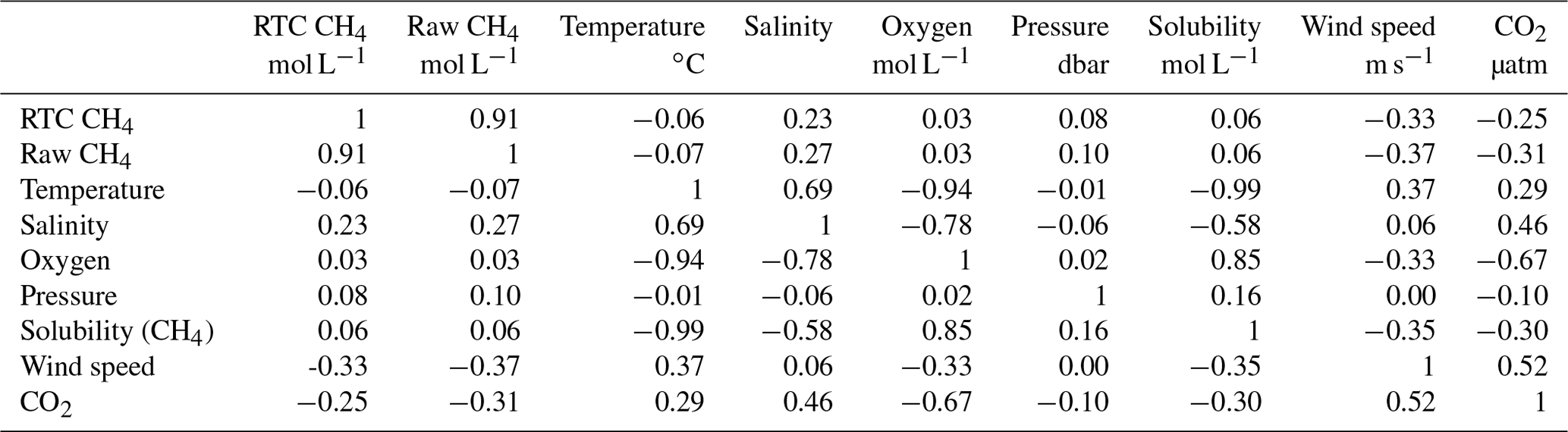
Table 1 Correlation coefficients between variables at O₉₁. The terms RTC CH₄ and raw CH₄ refer to response-time-corrected and untreated CH₄ data, respectively (Sect. 2 and Appendix B).

The high power consumption of the Contros HydroC CH₄ and CO₂ sensors required a power cycling mode to allow for long-term monitoring while simultaneously capturing rapid short-term variability. Partial pressure of CH₄ and CO₂ was therefore measured continuously for 24 h every 21 d and for 1 h every day (see Table B1). Methane concentration data were corrected for slow response time onto a 3 min interval grid and converted to absolute concentration following Dølven et al. (2021), which is the default “CH₄ concentration” discussed and described in this text (see Appendix B). Faulty pumps in the CO₂ sensors ambiguously increased the response time, which prevented response time correction, making CO₂ data suitable only for long-term qualitative analysis.

Uncertainty ranges for the CH₄ sensor data are reported as 95  % confidence intervals and typically vary between 5  % and 20  % (Fig. B1b). We did not perform any post-validation and/or intermittent validation. Although always an advantage for all sensors in long-term deployments, such validation is not a requirement for the TDLAS-based sensor (as opposed to NDIR), due to its high long-term stability. Standard post-processing (e.g., inspection of metadata such as internal pressure and temperature) and evaluation of fit residuals in the response time correction procedure (see Appendix B and Dølven et al., 2021) also indicated consistent sensor behavior throughout the deployments. It is also worth noting that the current paper is concerned with large changes and high concentrations, and we are confident that the quality of the response-time-corrected Contros HydroC CH₄ data is sufficient to support the inferences described herein.

We calculated correlation coefficient (R) matrices to give a first-order overview of the linear relationships between the measured parameters. We mapped the flares in the area using single-beam echo sounder data collected during the observatory recovery cruise in 2016 (CAGE 16-4, Fig. 1) and estimated gas flow rates using the FlareHunter software (Veloso et al., 2015). Additionally, we obtained 10 m wind reanalysis data from the ERA-Interim database.

We calculated seawater density (McDougall and Barker, 2011) and CH₄ solubility (Kossel et al., 2013) using the CTD data. A CTD cast (SBE plus 24 Hz) prior to the O₉₁ recovery (6 May 2016) showed a salinity drift in the conductivity sensor of around −0.4 (here and elsewhere in the paper, salinity values are practical salinity). Post-calibration inspection of the conductivity signal and potential water mass mixing end-members indicates that this might have been caused by mud pollution occurring in late 2015 or early 2016.

3 Results

3.1 Time series at site O₉₁

Dissolved CH₄ concentration at site O₉₁ ranged from 5 ± 3 nmol L⁻¹ (6 December in 2015) to 1748 ± 142 nmol L⁻¹ (20 August in 2015) (Fig. 2a and Appendix C), with 2.5 and 97.5 percentiles of 16 and 785 nmol L⁻¹. The data follow a nearly lognormal distribution, with a mean and median of 227 and 165 nmol L⁻¹, respectively, and interquartile range of 88–334 nmol L⁻¹. Large variations (> 100 up to almost 1000 nmol L⁻¹) in CH₄ concentration occurred on short timescales (< 1 h) throughout the measurement period (see Fig. 2a, d and all 24 h periods in Appendix C), with an average range for all 24 h periods of 840 nmol L⁻¹ and a median rate of change (ROC) of 3.2 nmol L⁻¹ min⁻¹. We also observe a long-term trend of decreasing running median (2-week window) concentrations towards winter, from 495 nmol L⁻¹ in July–August 2015 to 53 nmol L⁻¹ in January 2016 (Fig. 2). There was a relatively weak but significant negative correlation between the wind speed and CH₄ concentration ($R_{\mathrm{RTC}}=-\mathrm{0.33}$) but otherwise weak to non-existent linear relationships between CH₄ concentration and the measured ocean parameters (Table 1).

CO₂ averaged 403 µatm with an increase towards mid-November 2015 (∼ 410 µatm) and then a decrease until 6 May (∼ 391 µatm) in 2016 (Fig. 2a). CO₂ dropped to ∼ 305 µatm on 24 August, concurrent with a rapid decrease in salinity (−0.5), increase in temperature and oxygen, and high CH₄ concentration. The increase in oxygen rules out methanogenesis. Instead, there might be at least two explanations for the reduction of CO₂ and enrichment of CH₄: (i) water column mixing, which brings oxygen-rich, warm and fresh surface water to deeper depths (and with it CO₂-depleted water), or (ii) methane enrichment by zooplankton following the summer bloom.

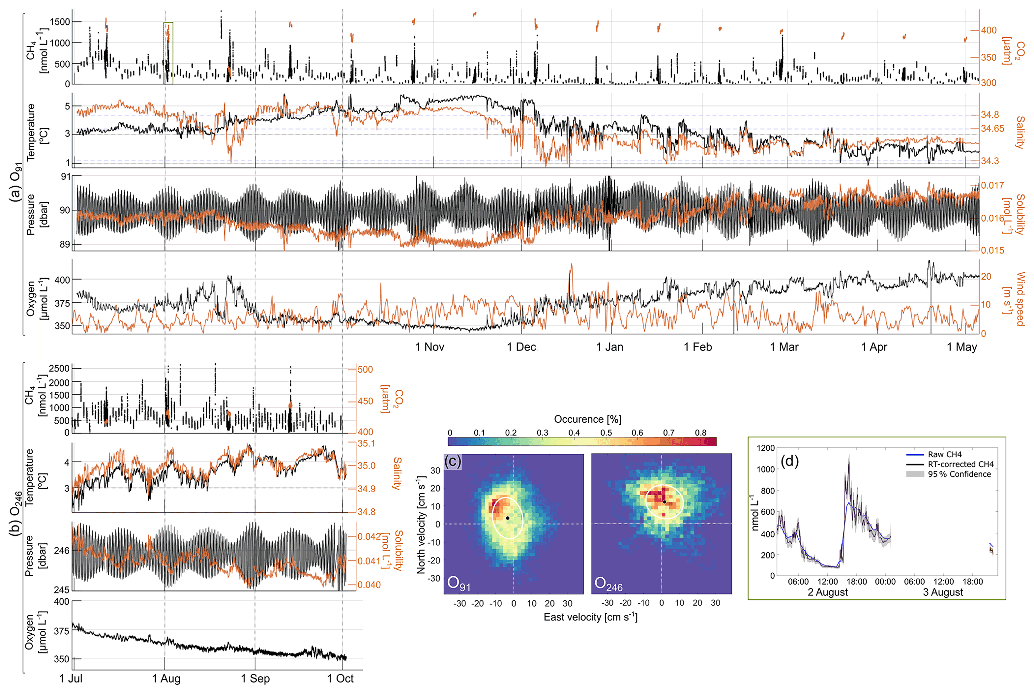
Figure 2 Time series from (a) O₉₁ and (b) O₂₄₆ showing response-time-corrected (see Appendix B) CH₄, CO₂, temperature, salinity, pressure, CH₄ solubility, oxygen and wind speed (10 m) data. The O₂₄₆ data are truncated due to an electrical malfunction in the system on 3 October. (c) A 2 d histogram and 1 SD variance ellipse of bottom current velocity (81 m depth at O₉₁ and 236 m depth at O₂₄₆) and (d) an example of 24 and 1 h (2 and 3 August) CH₄ concentration measurement period from O₉₁ (green box). All 24 h measurement periods are shown in Appendix C. Note the different scales between O₉₁ and O₂₄₆.

Bottom water temperature increased steadily from ∼ 3 in July 2015 to ∼ 5.5 ^∘C in October–November 2015, with occasional sharp shifts (T±1 ^∘C) occurring within hours to days (Fig. 2b). Temperature then decreased from the beginning of December 2015 to ∼ 1.8 ^∘C at the end of the deployment in May 2016, showing more frequent and stronger episodes of rapid temperature shifts (T±2 ^∘C also occurring over hours or days). Despite uncertainty in salinity data, it is worth noting that these rapid shifts in temperature and salinity were reproduced by the Svalbard 800 model in the same area (Silyakova et al., 2020) by eddy activity.

Hydrostatic pressure was mostly governed by tides (94.5 % of variance) with a dominant semi-diurnal M2 tide (M2 refers to a tidal constituent with period 12.42 h; see, e.g., Gerkema, 2019). Amplitudes varied from ∼ 1.2 to 1.5 m during neap and spring cycles (Fig. 2c).

The calculated CH₄ solubility decreased from 0.016 mol L⁻¹ in July 2015 to 0.015 mol L⁻¹ at the end of November 2015 and increased to almost 0.017 mol L⁻¹ in May 2016 (Fig. 2c). This long-term trend was mainly caused by temperature variability ($R=-\mathrm{0.99}$), while tidal pressure changes caused a semi-diurnal variation of $\pm \sim$0.005 mol L⁻¹.

Dissolved O₂ decreased from ∼ 385 µmol L⁻¹ in July 2015 to ∼ 350 µmol L⁻¹ at the beginning of December 2015 and increased to ∼ 400 µmol L⁻¹ towards 6 May 2016 (Fig. 2d) and followed temperature inversely ($R=-\mathrm{0.94}$), with similar long- and short-term variability.

The averaged bottom water current (81 m above the seafloor) was 4 cm s⁻¹ in a northwestward direction (321^∘ N) (Fig. 2c). The current usually had one counterclockwise rotation every 23.93 h period, corresponding to the diurnal K1 tidal constituent (tide with period 23.93 h; see Gerkema, 2019) with a secondary semi-diurnal (M2) modulation.

3.2 Time series at site O₂₄₆

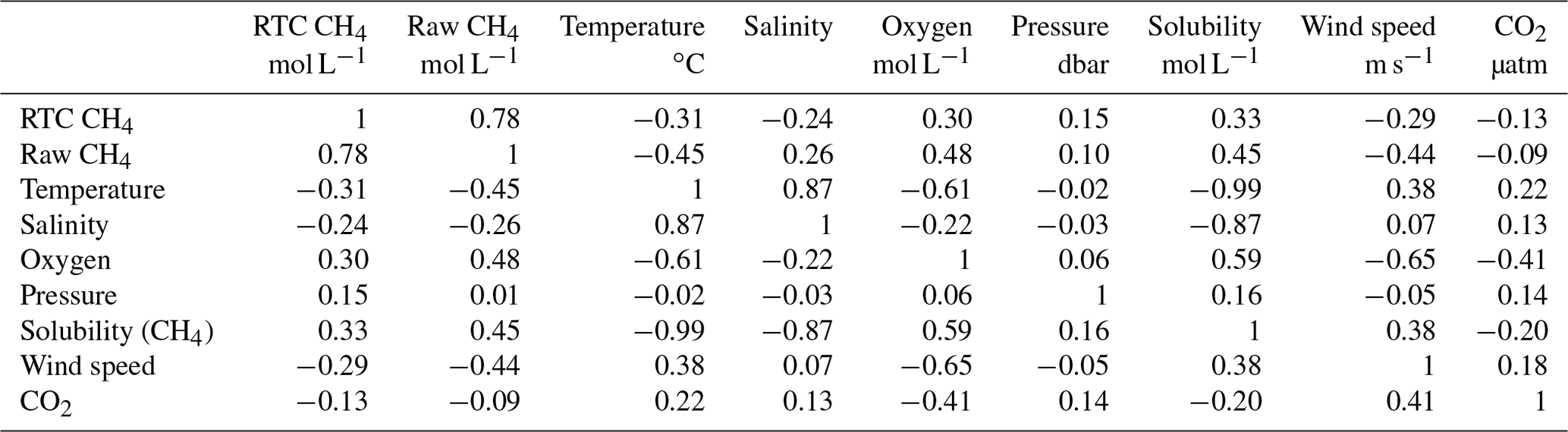
CH₄ concentration at site O₂₄₆ ranged from 10 ± 3 nmol L⁻¹ on 21 September 2015 to 2727 ± 182 nmol L⁻¹ on 18 August 2015, with 2.5 and 97.5 percentiles of 107 and 1374 nmol L⁻¹. The data approximately follow lognormal distribution with average and median of 577 and 600 nmol L⁻¹, respectively, and an interquartile range of 293–721 nmol L⁻¹. The median ROC of CH₄ (31 nmol L⁻¹ min⁻¹) was almost 20 times higher than site O₉₁ (Fig. 2b and Appendix C). There was also clear diurnal periodicity in CH₄ concentration at O₂₄₆. The long-term trend (2-week running mean) shows decreasing concentrations until 3 October 2015 (end of the measuring period, Fig. 2b). Dissolved O₂ decreased from ∼ 380 to ∼ 300 µmol L⁻¹ and was negatively correlated with water temperature ($R=-\mathrm{0.61}$; see Table 2 for the complete correlation matrix).

Table 2 Correlation coefficients between variables at O₉₁. The terms RTC CH₄ and raw CH₄ refer to response-time-corrected and untreated CH₄ (see Sect. 2 and Appendix B).

Temperature and salinity increased from ∼ 2.5 to ∼ 4.0 ^∘C and ∼ 34.85 up to ∼ 35.0, respectively, from the deployment until October 2015 (Fig. 2b), with Atlantic water being dominant throughout the measuring period. Rapid shifts of around ± 1 ^∘C and 0.05 salinity occurred occasionally over a period of hours to days.

Variance in hydrostatic pressure was mainly explained by the tides (95.2 %), which were mainly governed by the semi-diurnal M2 tide, with weaker diurnal and fortnightly modulation (Fig. 2b). Changes in pressure varied from ∼ 1.2 to ∼ 1.5 m during periods of neap and spring tide.

Being governed mainly by temperature ($R=-\mathrm{0.99}$), CH₄ solubility dropped from 0.042 to 0.040 mol L⁻¹ from the deployment in July until October 2015, with a semi-diurnal variation of ∼ 0.005 mol L⁻¹ due to tidal changes in hydrostatic pressure.

The averaged current was ∼ 10 cm s⁻¹ northward (7^∘ N) (Fig. 2c). Variability in the along-slope current (−10^∘ N direction) was strongly related to the semi-diurnal M2 tidal component, while the cross-slope currents were governed by the diurnal K1 frequency. The bottom water current rotated counterclockwise with a period of 23.93 h (K1 tidal constituent) and semi-diurnal modulation in the along-slope component. Dissolved CH₄ concentration was weakly anti-correlated with wind speed ($R=-\mathrm{0.29}$), temperature ($R=-\mathrm{0.31}$), and salinity ($R=-\mathrm{0.24}$) and positively correlated with CH₄ solubility (R=0.33) and oxygen (R=0.3).

4 Discussion

4.1 CH₄ variability

Combining mapped flares and flow rates from the recovery cruise (May 2016) with bottom water current velocity (9 m above the seafloor) reveals that CH₄ concentration was strongly affected by whether water was advected from areas where we mapped strong or weak seepage in May 2016 (Fig. 3). Strong seeps (flow rate > 200 mL⁻¹ min⁻¹) were mainly located between ∼ 30 and 80 m to the north or northeast of site O₉₁, and only weak and more distant seepage was observed southwest of the observatory (Fig. 3a). Consequently, the averaged CH₄ concentration from water coming from northeast was ∼ 440 nmol L⁻¹, while water from the southwest averaged ∼ 100 nmol L⁻¹. Similarly, a strong CH₄ seep (flow rate ∼ 1200 mL min⁻¹) was mapped ∼ 40 m north of site O₂₄₆, making water advected from this direction highly elevated in CH₄, with an average of ∼ 1400 nmol L⁻¹ compared to the overall average of 577 nmol L⁻¹ (Fig. 3b). The rapid changes in dissolved CH₄ can to a high degree be explained by this relationship, due to the high variability in ocean current velocity. That this relationship holds for most of the measuring period also shows that even though observed average concentrations are lower in winter months, the seep configuration did not change significantly from July 2015 to May 2016, and dissolved CH₄ was efficiently dispersed in relatively high concentrations in the whole seepage area.

Furthermore, daily CH₄ concentrations at site O₉₁ were higher on average than the 24 h measurements (313 vs. 200 nmol L⁻¹). This can be explained by the comparable measurement periodicity (24 h) and tidal periodicity (23.93 h) in the ocean currents, resulting in predominantly eastward advection during daily measurements, thus systematically transferring water from a weak seepage area (Fig. 3). We did not observe this effect at site O₂₄₆, most likely due to less tidal variance in the current direction (Fig. 2b). Nonetheless, this systematic tide-induced bias on the daily measurements at site O₉₁ highlights the importance of taking the oceanographic conditions into account to avoid misinterpretation of variability.

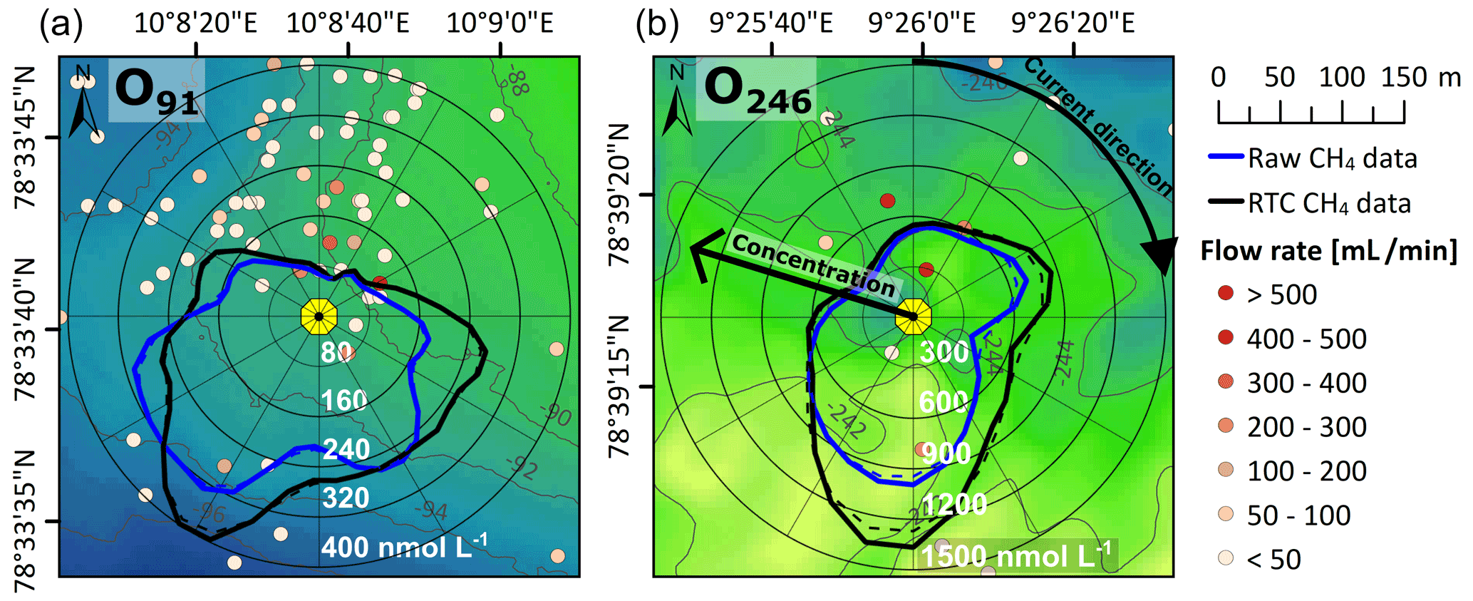
Figure 3 O₉₁ (a) and O₂₄₆ (b) location (yellow dot) and flow rates from flares mapped in their vicinity during CAGE 16-4 (color scale). Background color (green and blue) illustrates seafloor bathymetry. The compass diagram shows the relationship between ocean current direction (angle) and CH₄ concentration (distance from center; black is response-time-corrected (RTC) data, and raw data are in blue).

Since currents are mostly northward and seepage is mostly located to the north of both observatories, averaged measured CH₄ concentrations are likely lower than the average over the immediate surrounding area (Fig. 3). Despite this, the observatory data show higher average CH₄ concentrations than previously reported. In the area surrounding site O₉₁, Silyakova et al. (2020) reported average concentrations of 92, 70 and 61 nmol L⁻¹ in June 2014, July 2015 and May 2016, respectively, based on discrete water sampling. Averaged CH₄ concentrations measured at site O₉₁ in July 2015 and May 2016 were 566 and 110 nmol L⁻¹, respectively, i.e., around 8 and 2 times higher than values reported by Silyakova et al. (2020), respectively. The maximum CH₄ concentration at O₉₁ of 1748 ± 142 nmol L⁻¹ on 20 August 2015 also significantly exceeds the previously maximum recorded concentration in the area of 480 nmol L⁻¹ (July 2014, Silyakova et al., 2020). At site O₂₄₆ the August 2016 average (564 nmol L⁻¹) was 8 times higher than what Gentz et al. (2014) found in August 2010 (70 nmol L⁻¹) using an altimeter-controlled CTD towed at 2 m above the seafloor. The maximum concentration in August 2016 also significantly exceeded previous observations, with 2661 ± 163 nmol L⁻¹ compared to 524 nmol L⁻¹ measured by Gentz et al. (2014).

These differences could be a result of temporal, local or regional differences in CH₄ concentration. However, strong vertical gradients in dissolved CH₄ are well documented at both seep sites (Gentz et al., 2014), and our sensors measured closer to the seafloor (1.2 m above seafloor) compared to Gentz et al. (2014) (2 m above seafloor) and Silyakova et al. (2020) (5 to 15 m above seafloor). Additionally, the observatories were deployed close to seeps using a launcher, as opposed to “blind” water sampling from a shipborne rosette. Methane was also measured in situ, thereby avoiding potential CH₄ outgassing after retrieval of water samples (Schlüter et al., 1998).

Dissolved CH₄ within shallow seep sites where gas can bypass the oceanic sinks often present heterogeneous distribution and rapid temporal variability (Gentz et al., 2014; Myhre et al., 2016a). Our results show that the temporal variability at the two seep sites is higher than previously reported and that changing ocean currents and configuration of nearby seeps are major contributors. This high short-term variability introduces a conceptual error in studies relying on discrete water sampling (e.g., to calculate inventories) because the time required to conduct the survey (measured in days) is much longer than large temporal variations in concentration (up to an order of 10³ nmol L⁻¹ within hours).

Figure 4 Relative standard error of the mean for different numbers of samples N for O₉₁ 24 h data, data presented in Silyakova et al. (2020) (“June-14”, “July-15”, “May-16”), and O₂₄₆ 24 h data (in black). Relative standard deviation (corresponding to the standard error with N=1) is given in the legend (σ_rel). * Data from Silyakova et al. (2020) calculated assuming that the sample distribution resembles the underlying distribution (see Appendix D).

We can obtain a first-order constraint on errors caused by short-term variability in a hypothetical water sampling survey using the 24 h time series from the observatories. We assume the hypothetical survey seeks to find the average concentration in the bottom layer of the seep site. The expected error can then be found by calculating the standard error of the mean (SEM) for a given number of samples N using the 24 h time series as an underlying distribution representing the sub-daily variability of the seep site (Fig. 4; Appendix D contains a detailed outline of the methodology). Even though surveys often require more than 24 h to complete (2–3 d in Silyakova et al., 2020), a majority of processes causing short-term variability have periods below or at ∼ 24 h (for instance tides and many turbulent eddies; see, e.g., Sect. 3.2 and 3.1 and Talley et al., 2011), likely making the daily distribution relevant also for surveys with longer duration. We compared SEM calculations based on the observatory 24 h time series with SEM calculations for the bottom water (∼ 5 m above the seafloor) discrete water sample data used for average and inventory estimates of the O₉₁ seep site in Silyakova et al. (2020) (also included in Fig. 4).

The absolute SEM (in nmol L⁻¹) is generally higher for time series with higher averaged concentrations, making the relative SEM cluster well, with gradually diminishing range for increasing N (an inherent property of the SEM, e.g., 12 %–45 % for N=10, 9 %–30 % for N=30, Fig. 4). The SEM of the data from Silyakova et al. (2020) is similar to the SEM of the 24 h time series, with a common range of 5 %–15 % expected error for surveys with N∼60 samples (N=64, 62, and 63 in Silyakova et al. 2020). It should be noted that the comparison with data from Silyakova et al. (2020) has caveats, e.g., that the observatory data do not contain errors due to spatial variability and an assumption of representative short-term temporal variability at the observatory sites (see also Appendix D).

Evidently, detailed surveys of individual seep sites, such as the study by Silyakova et al. (2020), can provide reasonable estimates of local inventories (< 15 % uncertainty) despite high short-term temporal variability. However, it is important to note that the area investigated in Silyakova et al. (2020) was densely mapped and homogeneous in the sense that it is an area where seepage is well documented (Silyakova et al., 2020). Interpolation or averaging across larger regions where the amount of seepage is mostly unknown can result in considerable errors due to false interpolation assumptions and amplification of individual measurement errors, which can be large (expected errors up to ∼ 140 % for single measurements; see listed standard deviations in Fig. 4). These effects can potentially explain some of the discrepancies in estimates of oceanic CH₄ inventories and fluxes.

Our findings stress the importance of sufficiently dense mapping and knowledge about the underlying seep condition when collecting water samples for inventory estimates. They also highlight the advantage of towed or autonomous instrumentation capable of providing continuous CH₄ data, giving considerably better coverage and representation of the CH₄ distribution in less time (e.g., Sommer et al., 2015; Grilli et al., 2018; Canning et al., 2021). Assuming a distribution that better reflects the uneven spread of CH₄ when applying interpolation and extrapolation techniques could also limit estimation errors. Future studies should investigate how initial errors due to short-term and small-scale variability propagate via different upscaling techniques and how these errors can be mitigated.

4.2 Hydrostatic pressure

Tidal changes in hydrostatic pressure can trigger CH₄ release by build-up of CH₄ in sediment pore water at rising tide and subsequent release when pore pressure decreases at falling tide, as observed at the Hikurangi Margin (Linke et al., 2009) and Clayoquot Slope (Römer et al., 2016). Our study sites differ from these sites in depth (they are >600 m) and in tidal amplitude (4 m at Clayoquot Slope compared to 1.5 offshore Prins Karls Forland). Linke et al. (2009) and Römer et al. (2016) also observed bubbles hydro-acoustically, while we measure dissolved CH₄, which is strongly affected by the (also tidally dependent) current direction (Fig. 3).

To evaluate the effect that hydrostatic pressure changes have on the in situ concentration, we need to constrain the variance caused by changing current directions (since they operate in the same frequency domain). To do this, we first binned the CH₄ concentration data into overlapping bins defined by the current direction at the time when the measurement was obtained and calculated standard scores (the number of standard deviations each value deviates from the sample mean; see, e.g., Kreyszig, 1979) for the data in each bin. We used larger current direction intervals for O₂₄₆ due to the shorter data set, with a 12^∘ window for O₉₁ and a 30^∘ window for O₂₄₆. This resulted in a data set (i.e., the standard scores from all bins) effectively unrelated to the current direction. We then binned all the standard-scored CH₄ data according to when the data were collected in relation to the M2 governed tidal cycle peak using overlapping 30 min bins (the M2 tide explains 79.2 % and 80.3 % of the pressure variance at O₉₁ and O₂₄₆, respectively). Average and median values were calculated for each bin, giving the averaged or median normalized dissolved CH₄ value (standard score) for each current velocity defined data bin as a function of the M2 tidal cycle (Fig. 5). This partial decoupling of variability in hydrostatic pressure and current direction was possible since the bottom water current and hydrostatic pressure changes had different dominant tidal constituents; i.e., the current was mainly dominated by the diurnal K1 constituent (∼ 23.91 h period), while the M2 tide is semi-diurnal (12.42 h period).

A strong effect of the hydrostatic pressure on local seepage should elevate the standard scores at decreasing pressure (from 0 to 6.2 h, i.e., in the right half of Fig. 5), which we observe at both observatories. However, we observe stronger peaks at increasing hydrostatic pressure (−3 h) at site O₉₁ and at the M2 peak (0 h) at site O₂₄₆, which contradicts this hypothesis. This does not mean that there is no effect of hydrostatic pressure changes but rather that the seepage in the area is widespread at both falling and rising tide conditions. The high variability caused by the strong effect of current direction also makes it particularly challenging to detect moderate changes in seepage intensity.

Figure 5 Median and averaged standard scores of CH₄ binned according to bottom water current direction and according to where the data were sampled in relation to the phase of the M2 pressure tide.

4.3 Bottom water temperature

Bottom water temperature can affect CH₄ release by altering hydrate stability and CH₄ solubility in pore water and the water column (Sloan, 1998; Jansson et al., 2019a). Seasonal CH₄ release variability resulting from temperature variations in the bottom water has been linked to migration of the gas hydrate stability zone (GHSZ) and hydrate dissociation further offshore at ∼ 390 m water depth (Berndt et al., 2014; Ferré et al., 2020). Our observatories were deployed in areas too shallow for gas hydrate to form. However, inversely varying seepage intensity between seepage at the GHSZ depth (390 m) and site O₂₄₆ can suggest that these areas are fed by the same hydrocarbon source and that hydrates seasonally block the lateral pathways between these seep sites (Veloso-Alarcón et al., 2019). This is in agreement with the observed long-term (∼ 3 months) negative correlation between bottom water temperature and dissolved CH₄ at site O₂₄₆ ($R=-\mathrm{0.31}$). It should be noted that the same relationship is observed at O₉₁; however, no geophysical data are available from this area due to the shallow depth.

Tidal pressure variations can affect CH₄ release via pore water solubility (Sect. 4.2), but on longer timescales CH₄ solubility is almost exclusively a function of water temperature. Higher CH₄ solubility implies more CH₄ dissolved in pore water and within bubble streams, potentially increasing the amount of CH₄ dissolved in bottom water. A small but significant (R=0.33) positive correlation between CH₄ solubility and concentration at site O₂₄₆ and site O₉₁ (considering the same time period, i.e., until 3 October in 2015) could indicate such an effect. This is also an alternative explanation for the negative correlation between temperature and CH₄ concentration at site O₂₄₆.

4.4 Pore water seepage

Short-term temperature increase further offshore (390 m depth) has been linked with release of warm, CH₄-rich fluids from the sediments triggered by short-duration seismic events (Franek et al., 2017). This means that increased CH₄ concentration should be accompanied by increased water temperature and reduced salinity due to admixture of warmer, less saline pore water. We compared short-term anomalies (i.e., deviations from daily means) in these three variables in the 24 h data sets at both seep sites but found no corroborating evidence for this hypothesis. Instead, the covariance between current velocity and temperature and salinity anomalies indicates that short-term variability is mainly caused by cross-shelf exchange of Atlantic water in the West Spitsbergen Current and the colder, fresher Arctic water in the Coastal Current due to eddies (Hattermann et al., 2016). It also indicates that CH₄ release comes mainly from bubble dissolution and not from pore water seepage.

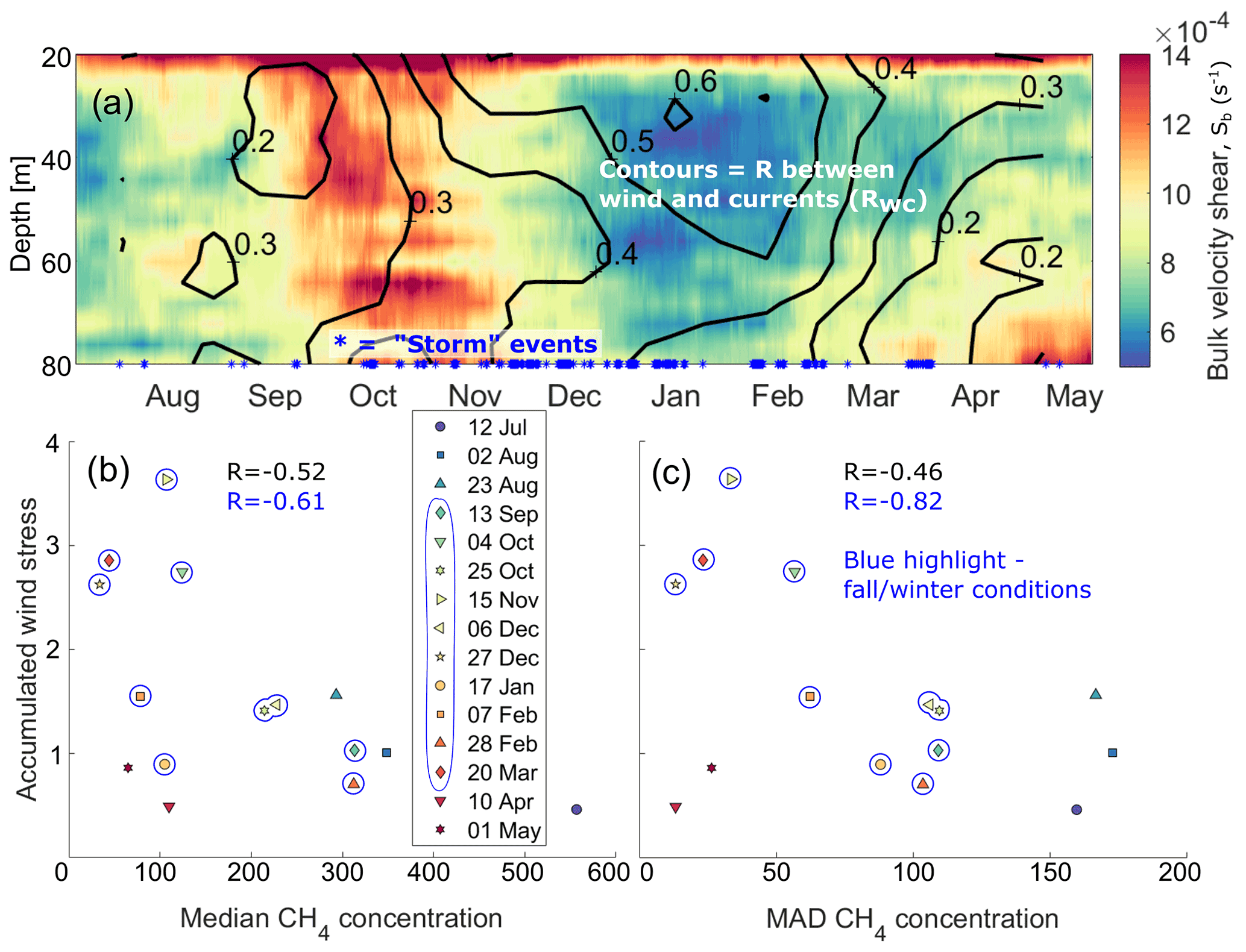
Figure 6 (a) Bulk velocity shear (ΔH=8 m) and two-dimensional correlation with wind stress (contours). Relationships between 5 d accumulated wind stress and median (b) and median absolute deviation (c) of CH₄ concentration for 24 h data periods. Persistent wind events with speeds of more than 10 m s⁻¹ in periods over 6 h are indicated with blue stars along the x axis of panel (a). Blue highlights fall and winter water column conditions as described in the text.

4.5 Seasonal variation of CH₄ distribution at site O₉₁

Low release of CH₄ to the atmosphere from the O₉₁ seep area during summer despite high seabed influx has been explained by suppression of vertical mixing by strong stratification (Myhre et al., 2016a) or absence of mechanical forcing such as wind stress (Silyakova et al., 2020). However, in fall and winter, the water column offshore Prins Karls Forland is expected to have more horizontal and vertical mixing due to weaker stratification from cooling or sea ice formation (Tverberg et al., 2014), baroclinic instability in the frontal structures of the West Spitsbergen Current (von Appen et al., 2016; Hattermann et al., 2016), and more frequent storms (Nilsen et al., 2016).

We expect lower CH₄ variability and lower CH₄ concentration during periods of high mixing and dispersion due to weaker horizontal and vertical gradients and more efficient dispersion of CH₄ away from sources. We use three sets of parameters to evaluate long-term changes in the amount of mixing in the water column (see Appendix E): (i) the 4-week averaged bulk velocity shear (S_b), (ii) the two-dimensional correlation between wind stress and current velocity (R_WC), and (iii) the number of stormy days as defined by persistent winds > 11 ms⁻¹ lasting longer than 6 h (Fig. 6). Calm weather and low S_b and R_WC until mid-September 2015 indicate a stable water column with limited mixing in the bottom waters. From mid-September, S_b increased and stayed high until mid-November, together with a gradual increase in R_WC that can be attributed to a gradual breakdown of stratification and increasing number of storm events (Fig. 6a). R_WC remained high (R_WC>0.5 at 60 m depth) until March 2016, indicating a significant effect of wind forcing in the water column. From March until observatory retrieval, R_WC decreased to <0.2 below 50 m depth while S_b increased below 60 m depth, indicating available energy for mixing in the bottom waters.

We quantified CH₄ variability during the 24 h measurements using the median absolute deviation (MAD) and used the median as a measure of the amount of dissolved CH₄. The three 24 h periods collected during the calmer period prior to mid-September had high median concentration (> 300 nmol L⁻¹) and the overall highest variability (MAD > 160 nmol L⁻¹), as expected for low mixing conditions (Fig. 6b and c). From mid-September until the end of March (i.e., fall and winter seasons), the 24 h CH₄ concentration time series had generally lower MAD and median concentration. In this period, CH₄ variability and median also showed a good statistical relationship with the 5 d accumulated wind stress ($R=-\mathrm{0.82}$ for MAD and $R=-\mathrm{0.61}$ for median concentration), indicating that wind forcing has a deep impact on mixing and redistribution of CH₄ in the water column (which also fits well with a high R_WC). The two last 24 h CH₄ time series (10 April and 1 May) had low median concentration, which could be explained by the absence of stratification (Silyakova et al., 2020) and generation of mixing from the observed increase in S_b.

Accumulated wind stress, S_b and R_WC are only limited indicators of water column dispersion and mixing. Nonetheless, the relationship between these parameters and the MAD and medians of the 24 h period CH₄ time series gives a good indication of the seasonal cycle of distribution and vertical transport of CH₄: strong stratification, less wind forcing and eddy activity in summer limit mixing and prevent CH₄ from reaching the atmosphere. However, in fall and winter, reduced stratification makes the water column more prone to mixing, and distribution of CH₄ seems to be strongly linked with wind forcing from September to April.

5 Conclusions

Time series of dissolved CH₄ at both lander locations show considerably higher CH₄ concentrations (up to 1748 ± 142 nmol L⁻¹ at O₉₁ and 2727 ± 182 nmol L⁻¹ at O₂₄₆) than previously found in ship-based water sampling surveys (maximum of 482 near O₉₁ and of 564 near O₂₄₆). The time series also uncover high CH₄ variability (up to ∼ 1000 nmol L⁻¹) within short timescales (<24 h), highlighting the potential uncertainty of flux and inventory estimates based on interpolation and extrapolation techniques relying on, e.g., an assumption of linearity. We calculated the standard error of a mean estimate based on a hypothetical discrete water sampling survey based on a range of samples by using the 24 h time series as the underlying distribution. The results aligned well with previous discrete water sampling surveys in the area, giving a standard error of the mean of 5 %–15 % for ∼ 60 samples.

Variability can be linked to directional ocean current variations occurring at tidal timescales, which shows the importance of taking the current direction and seep locations into account when interpreting intense seep site observations. The persistent relationship between current direction and location of seeps during recovery shows that there was seepage throughout the year and that the seep configuration was relatively constant.

We did not observe a direct effect of tidal pressure variations on CH₄ release, but this could be hidden by the strong effect of variations in current direction. A negative (long-term) correlation between temperature and dissolved CH₄ at O₂₄₆ is in agreement with the hypothesized seasonal blocking of lateral CH₄ pathways in the sediments (Veloso-Alarcón et al., 2019) but could also be explained by increased CH₄ solubility in the water column.

Short-term, small-scale variations in temperature and salinity were not linked with increased amounts of dissolved CH₄, but rather with cross-frontal exchange of water masses due to eddies.

We observed a seasonal cycle in the characteristics of the 24 h time series that fits with seasonal changes in dispersion and mixing characteristics of the water column. Higher CH₄ concentration and variability in early fall, when stratification was strong, was followed by lower median concentrations and variability in late fall and winter when the water column was more affected by mixing. In late fall and winter, wind forcing was statistically coupled to the concentration and variability of CH₄, probably due to weaker water column stratification.

When estimating the atmospheric impact of a particular CH₄ source based on sparse measurements, it is crucial to have some constraints on the temporal and spatial variability. These constraints can either be direct knowledge about variability itself or how inventory and fluxes are affected by related physical and/or chemical parameters. We observed considerable temporal and spatial variability at the two seep sites that need to be taken into account to obtain meaningful estimates of CH₄ fluxes or inventories. That no strong direct link was found with other oceanographic parameters illustrates the nonlinearity of the system, making careful interpretation of measurements important. Future studies should aim to identify the errors that arise via different upscaling and interpolation techniques and how these errors can be mitigated. Based on our observations, we suggest that uncertainties in CH₄ inventory and seep estimates can be mitigated by taking the local seep configuration, ocean currents and mixing rates into account and employing autonomous instrumentation capable of resolving the steep horizontal gradients in dissolved CH₄. This, alongside direct measurements of seepage by, e.g., acoustic instrumentation, can help constrain future estimates of CH₄ flux to the atmosphere from seabed seepage.

Appendix A: The K-Lander

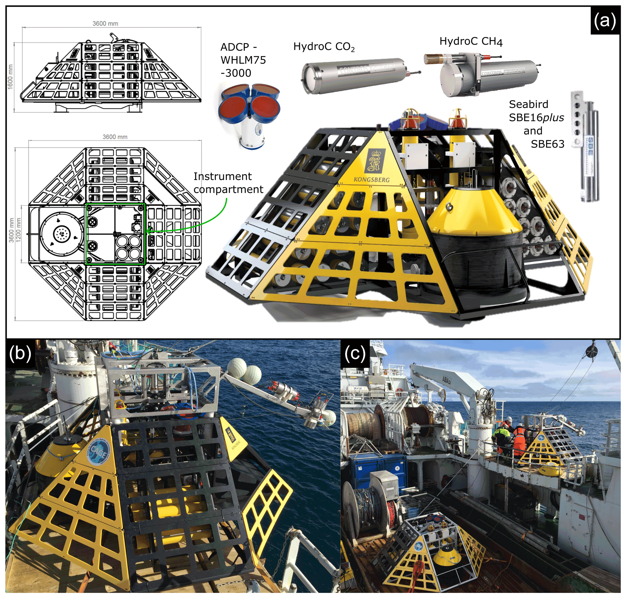
Figure A1 (a) The K-Lander is a 1.6 m high and 3.6 m wide trawl-proof stainless steel frame with multiple instrument mounts and batteries. The side panels are perforated to allow unobstructed water flow to the instruments inside the structure. See Appendix B for details on instrumentation. (b) One of the K-Landers during deployment with a launcher mounted on top and camera system mounted on a boom for visual control of landing area. (c) The two K-landers before deployment.

Appendix B: Measurement intervals, general post-processing and data

The CTD (oxygen sensor) and ADCP conducted measurements every 4 and 9 min, respectively, during the continuous monitoring of CH₄ and CO₂ measurements and every 21 and 29 min, respectively, during the rest of the deployment period (see Table B1 for acronyms, description and measurement accuracy). Salinity was measured on the practical salinity scale.

The upward-mounted ADCP measured ocean currents in 1 m bins with a bottom 7 m blank distance, where the topmost 20 % of the water column was disregarded due to side lobe interference. The high resolution, relatively short ensemble time (1 min) and potential presence of CH₄ bubbles in the water resulted in noisy data. We dampened the noise by first removing any data points with error velocities exceeding one short-term (1 week) standard deviation, smoothed the data using a second-order Butterworth low-pass filter with a 3 h cutoff period and a spatial (i.e., vertical) moving average filter with a 5 m Hann window (increasing the blank distance to 10 m). The accuracy of the ADCP data is therefore not explicitly constrained and is based on comparing current velocity frequency spectra before and after filtering, combined with averaged error velocity of the raw data (Table B1).

Since sensors were recording at different frequencies, chronological alignment of the data was carried out by identifying nearest neighbor data points or by resampling. For correlation coefficients, histograms and Fourier analysis, the data sets were resampled to a uniform 15 min or 1 h measuring interval depending on the sample frequency of the raw data, using a poly-phase anti-aliasing filter. Due to the power-cycling mode of the CH₄ and CO₂ sensors and differing sampling frequencies, some statistics were based on more data points than others (outlined in Table B1). Daily measurements of CH₄ were excluded from these statistics due to the high probability of systematic errors induced by periodic diurnal effects.

Harmonic analysis of hydrostatic pressure and ocean currents was done using t_tide (see Pawlowicz et al., 2002) and the fast Fourier transform.

We calculated the rate of change (ROC) in CH₄ concentration using the response-time-corrected CH₄ data and the absolute value of the three-point (9 min) finite differences to limit the effect of noise on the calculation.

The absolute concentration of CH₄ in the water (nmol L⁻¹) was estimated from the partial pressure of CH₄, pressure, temperature and salinity using Henry's law and Henry constants obtained from Harvey (1996) and the practical molar volume and gamma term from Duan and Mao (2006).

The CH₄ sensors were calibrated to relevant water temperatures prior to deployment. The TDLAS detectors (Contros GmbH, 2018) provide measurements with good selectivity (fit for purpose) and high long-term stability (intermittent calibration not necessary) and are unaffected by dissolved oxygen content (unless via complete depletion). Biofouling was also minimal at retrieval (due to the cold water and local setting), and the PDMS membranes are almost unaffected by cold water. Generally, we did no observations indicating issues with any of the sensors except for what has already been mentioned regarding the conductivity probe and electrical malfunction of O₂₄₆. Furthermore, we discarded all data recorded during instrument warm-up (i.e., when internal temperature was below correct operating temperature) before the individual measurement periods (the instruments were turned on ∼ 35 min prior to recording the data used in the analysis).

In the Contros HydroC CH₄ and CO₂ sensors, dissolved gases diffuse through a hydrophobic membrane into a gas chamber and equilibrate with the ambient environment. This results in the slow response time (e.g., τ₆₃∼50 min under certain conditions for our membrane and pump setup for the CH₄ sensor) and poor representation of the rapid changes in CH₄ we expected in our study area (Gentz et al., 2014; Myhre et al., 2016a). We therefore performed a response time correction for the dissolved CH₄ data following the methodology presented in Dølven et al. (2021), modulating the response time using the temperature data (effects of salinity on membrane permeability were not taken into account since these are negligible for the local ranges; see Robb, 1968). The CO₂ sensors had a faulty pump, which ambiguously increased the response time of the sensors, making response time correction impossible.

The response time correction was performed for each period individually (1 and 24 h, i.e., 377 periods), using the stated measurement accuracy of the instrument (2 µatm or 3 % of measured value, whichever is higher) as input uncertainty. We first identified the ideal Δt according to the maximum curvature point in the L curves of the 24 h measurement periods. These varied slightly between each measurement period but averaged close to 180 s (176.4 s). To keep the same measuring interval for all the CH₄ data, we therefore corrected all the data with a specified Δt of 180 s, which falls well within the bend of the L curve and should therefore safeguard a good balance between noise and model error (Fig. B1a). Inspection of model fit residuals showed a slight modulation following the variance in the signal, which is explained by our choice to use the same 3 min measurement grid across a relatively wide variance range, but the residuals were otherwise Gaussian. Although this is expected, it indicates that errors might be slightly overestimated for low-variance sections of the time series and vice versa for high-variance sections.

The uncertainty estimate varies depending on the amount of CH₄ measured by the TDLAS unit in the measurement chamber of the instrument. The distribution of the uncertainty estimates is shown as percentages in Fig. B1b. Estimated uncertainty ranged from 3 to 205 nmol L⁻¹ (95 % confidence, high for high concentrations in the measurement chamber and vice versa) or usually between 5 % and 20 %, although there were some outliers when the concentration was low and uncertainty estimate was high (Fig. B1b).

Table B1 Instruments mounted on O₉₁ and O₂₄₆ (see Fig. A1), measured parameters, height in meters above seafloor (masf), and stated accuracy. ADCP stands for acoustic Doppler current profiler. N shows the number of data points used for later multi-variable analysis of O₉₁ and O₂₄₆.

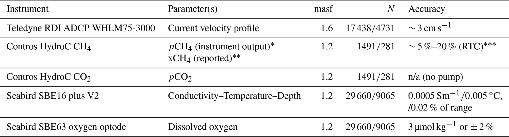
^* The Contros HydroC CH₄ outputs partial pressure from the internal gas chamber. ${}^{**}$ We report absolute concentration in seawater (nmol L⁻¹) using Henry's law. ${}^{***}$ We report accuracy only for response-time-corrected (RTC) concentrations (see Fig. B1) since the accuracy for untreated CH₄ concentration data is ambiguous due to the slow response time. n/a: not applicable.

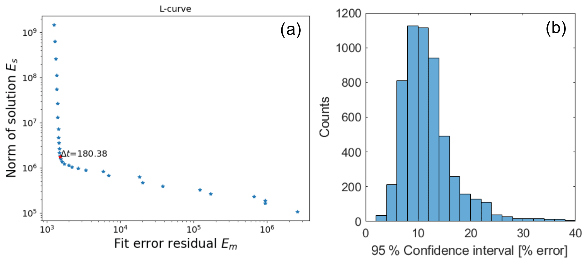
Figure B1 (a) L curve for response time correction of CH₄ data showing the location of the chosen Δt (180 s) for 6 May at O91. (b) Estimated relative (%) uncertainty for response-time-corrected CH₄ data (both observatories).

Appendix C: The 24 h measurements of CH₄

Figure C1 All 24 h periods of CH₄ concentration at O₉₁ using response-time-corrected data (black) with the uncertainty estimate (grey shading, 95 % confidence) and raw data (blue) from O₉₁.

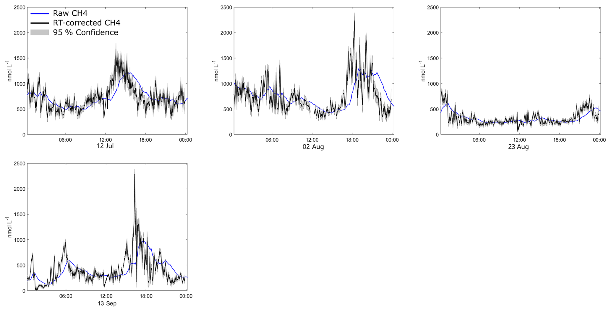
Figure C2 All 24 h periods of CH₄ concentration at O₂₄₆ using response-time-corrected data (black) with the uncertainty estimate (grey shading, 95 % confidence) and raw data (blue) from O₂₄₆.

Appendix D: Standard error of mean estimate due to temporal variability

To obtain the (theoretical) true dissolved CH₄ average or inventory for an area requires a known concentration everywhere at a single point T₀ in time. Considering a hypothetical ship-based discrete water sampling survey, any small-scale spatial variability not resolved by the sampling grid or localized (not seep-wide) short-term temporal variability occurring during the survey time can be considered a measurement errors for the purpose of the survey. Assuming that the water samples are sufficiently spaced out to be considered independent samples, the estimated average concentration from N samples in a particular depth layer at a seep site can be expressed as follows:

$$\begin{array}{}\text{(D1)}& {\displaystyle }E\left(m,{\mathit{ϵ}}_{\mathrm{t}},{\mathit{ϵ}}_{\mathrm{s}}\right)={\displaystyle \frac{{\sum }_{n=\mathrm{1}}^N\left(m+{{\mathit{ϵ}}_{\mathrm{t}}}_n+{{\mathit{ϵ}}_{\mathrm{s}}}_n\right)}{N}},\end{array}$$

where m is the average of the seep site at T₀, ϵ_t is error due to temporal short-term deviation from m at sampling time T₀+Δt and ϵ_s is spatial deviation in concentration from m. The expected standard error of $E(m,{\mathit{ϵ}}_{\mathrm{t}},{\mathit{ϵ}}_{\mathrm{s}})$ from the short-term temporal and spatial variability is then given by

$$\begin{array}{}\text{(D2)}& {\mathit{\sigma }}_{E\left(m,{\mathit{ϵ}}_{\mathrm{t}},{\mathit{ϵ}}_{\mathrm{s}}\right)}={\displaystyle \frac{\mathit{\sigma }}{\sqrt{N}}},\end{array}$$

where σ is the standard deviation of the distribution we sample from Ayyub and McCuen (2011). From Eqs. (D1) and (D2) we obtain

$$\begin{array}{}\text{(D3)}& {\mathit{\sigma }}_{E\left(m,{\mathit{ϵ}}_{\mathrm{t}},{\mathit{ϵ}}_{\mathrm{s}}\right)}={\mathit{\sigma }}_{E\left(m,{\mathit{ϵ}}_{\mathrm{t}}\right)}+{\mathit{\sigma }}_{E\left(m,{\mathit{ϵ}}_{\mathrm{s}}\right)}={\displaystyle \frac{{\mathit{\sigma }}_{\mathrm{t}}}{\sqrt{N}}}+{\displaystyle \frac{{\mathit{\sigma }}_{\mathrm{s}}}{\sqrt{N}}},\end{array}$$

where σ_t and σ_s are the distribution standard deviation related to temporal (ϵ_t) and spatial (ϵ_s) variability and ${\mathit{\sigma }}_{E(m,{\mathit{ϵ}}_{\mathrm{t}})}$ and ${\mathit{\sigma }}_{E(m,{\mathit{ϵ}}_{\mathrm{s}})}$ are the corresponding contributions to the standard error of the mean. Assuming the daily variance at the observatory is representative for the seep site, we can describe the expected error caused by sub-daily variability (all ϵ_t) in a scenario where a seep site is being sampled N times using the 24 h time series as the underlying distribution. In essence, we treat every measurement as having an associated probability distribution that is represented by the 24 h time series (which gives the sub-daily variability).

In the discrete water sample data presented in Silyakova et al. (2020), the underlying distribution is unknown, and we can only assume that the sample distribution resembles the underlying distribution, i.e., that

$$\begin{array}{}\text{(D4)}& {\mathit{\sigma }}_{E\left(m,{\mathit{ϵ}}_{\mathrm{t}},{\mathit{ϵ}}_{\mathrm{s}}\right)}\approx {\widehat{\mathit{\sigma }}}_{E(m,{\mathit{ϵ}}_{\mathrm{t}},{\mathit{ϵ}}_{\mathrm{s}})}={\displaystyle \frac{{\mathit{\sigma }}_{\mathrm{sampled}}}{\sqrt{N}}},\end{array}$$

where ${\widehat{\mathit{\sigma }}}_{E(m,{\mathit{ϵ}}_{\mathrm{t}},{\mathit{ϵ}}_{\mathrm{s}})}$ is the standard error estimate of the mean based on the sample distribution and σ_sampled is the standard deviation of the measurements. All three data sets, i.e., “June-14” (N=64), “July-15” (N=62) and “May-16” (N=63), have a similarly skewed distribution compared to what is found in the observatory data (see Fig. D1), which supports this assumption. The survey in Silyakova et al. (2020) required 2–3 d to complete, while the observatory data only concern sub-daily variability (24 h time series). Nonetheless, we believe the comparison is valid, since the known major contributors to short-term (timescales shorter than weeks) variability act on sub-daily (or at least ≤ daily) scales, such as the dominant frequencies in the ocean currents and pressure changes.

There is a clear relationship of increasing ${\mathit{\sigma }}_{E(m,{\mathit{ϵ}}_{\mathrm{t}},{\mathit{ϵ}}_{\mathrm{s}})}$ with increasing daily average, making relative ${\mathit{\sigma }}_{E(m,{\mathit{ϵ}}_{\mathrm{t}},{\mathit{ϵ}}_{\mathrm{s}})}$ a meaningful quantity to use, as opposed to absolute ${\mathit{\sigma }}_{E(m,{\mathit{ϵ}}_{\mathrm{t}},{\mathit{ϵ}}_{\mathrm{s}})}$. Additionally, for simplicity, we have not differentiated in the notation of the standard error of the mean (SEM) in the main text of the paper, referring to it as simply SEM in all situations.

It is also enlightening to consider the distribution of average estimates and how the skewed underlying distribution affects the distribution of average estimate errors for smaller N. We did this by simulating hypothetical surveys by random sampling from the 24 h data sets (Fig. D2), which shows the elevated probability of underestimating the average for estimates based on few samples (N≲30), i.e., that the median error is smaller than the average error. This is caused by an inheritance of the skewed underlying distribution in the CH₄ concentration data (see Fig. D2a). This also allows for severe overestimates due to the long right-hand-side tail of the distribution. For larger values of N (N≳30), average estimates tend towards being normally distributed, thus avoiding these effects (see Fig. D2b).

Error estimates of more complicated properties, such as the total CH₄ content in a volume of water based on interpolation techniques, require an assessment of the individual uncertainties of each measurement and how these errors propagate via, e.g., linear interpolation in the spatial domain. While not being explicitly applicable to inventory estimates, the σ_E still describes how random errors cancel out for larger values of N in evenly sampled grids, assuming this variability is representative for the seep site.

Figure D1 Distribution of CH₄ concentrations from the (a) June 2014, (b) July 2015 and (c) May 2016 data in Silyakova et al. (2020) and (d) from the 24 h data (all periods) at O₉₁. Note the different scale for the y axis between (a)–(c) and (d).

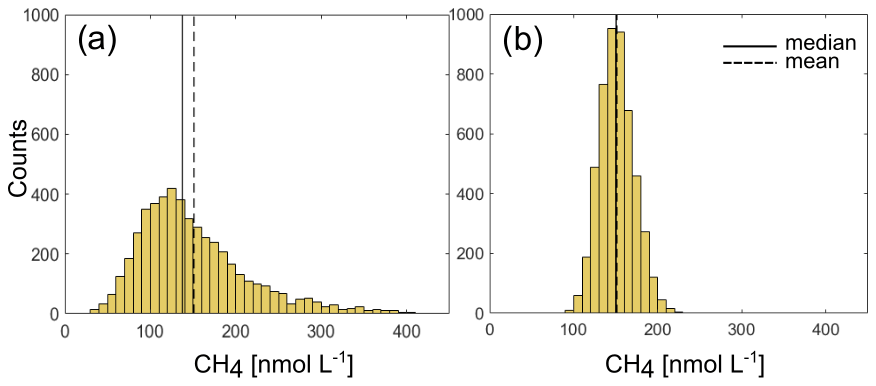
Figure D2 Histograms of simulated average estimates based on N=10 (a) and N=30 (b) samples from the 24 h data set from 23 August at O₉₁ showing the median and mean as vertical lines.

Appendix E: Bulk velocity shear and wind stress correlation

We calculated bulk wind stress using 10 m above sea level ERA-interim reanalysis wind data (Dee et al., 2011; Large and Pond, 1981). Water column bulk velocity shear S_b (see, e.g., Lincoln et al., 2016) was calculated as follows:

$$\begin{array}{}\text{(E1)}& S_{\mathrm{b}}^{\mathrm{2}}={\left({\displaystyle \frac{u_{\mathrm{u}}-u_{\mathrm{l}}}{h_{\mathrm{diff}}}}\right)}^{\mathrm{2}}+{\left({\displaystyle \frac{v_{\mathrm{u}}-v_{\mathrm{l}}}{h_{\mathrm{diff}}}}\right)}^{\mathrm{2}},\end{array}$$

where u_u, u_l, v_u and v_l refer to the eastward and northward ADCP velocity components in the upper (subscript u) and lower (subscript l) layer and h_diff is the vertical distance between layers. The direct effect of wind stress is usually confined to surface water, although indirect effects such as Ekman transport or overturning and the formation of eddies can facilitate currents and mixing at deeper depths (Cushman-Roisin and Beckers, 2011). The two-dimensional correlation coefficient R_WC between the wind and ocean currents was calculated using Kundu (1976) and the complex representations of the wind stress and de-tided current velocity vectors (τ_c and u_c, respectively) as follows:

$$\begin{array}{}\text{(E2)}& {\mathrm{R}}_{\mathrm{WC}}={\displaystyle \frac{\langle {\mathit{\tau }}_{\mathrm{c}}^{*}{\mathit{u}}_{\mathrm{c}}\rangle }{\langle {\mathit{\tau }}_{\mathrm{c}}^{*}{\mathit{\tau }}_{\mathrm{c}}{\rangle }^{\frac{\mathrm{1}}{\mathrm{2}}}\langle {\mathit{u}}_{\mathrm{c}}^{*}{\mathit{u}}_{\mathrm{c}}{\rangle }^{\frac{\mathrm{1}}{\mathrm{2}}}}},\end{array}$$

where 〈…〉 gives the normalized inner product of the vectors and ^* annotates the complex conjugate. We allow time lags of up to 15 h to account for the gradual and indirect effects of wind stress on the ocean currents. Both properties were estimated throughout the valid current velocity profile, but this was only done only down to 80 m depth due to the 8 m vertical distance between the defined layers used in the bulk velocity shear calculation.