the Creative Commons Attribution 4.0 License.
the Creative Commons Attribution 4.0 License.
 | 20 Dec 2022
Imminent reversal of the residual flow through the Marsdiep tidal inlet into the Dutch Wadden Sea based on multiyear ferry-borne acoustic Doppler current profiler (ADCP) observations
Johan van der Molen
Sjoerd Groeskamp
Leo R. M. Maas
The Dutch Wadden Sea is a UN World Heritage Site connected to the North Sea by multiple tidal inlets. Although there are strong tidal currents flowing through these inlets, the magnitude and direction of the residual circulation in the western Dutch Wadden Sea is important for sediment, salinity and nutrient balances. We found that the direction of this residual flow is reversing.
This residual circulation has been the subject of various studies since the 1970s, in which substantially different net volume fluxes were presented. Differences in tidal conditions in the main inlets, tidal rectification and meteorology were identified as driving mechanisms. Here we analysed almost 13 years of acoustic Doppler current profiler (ADCP) observations collected on the ferry crossing the Marsdiep tidal inlet in the Dutch Wadden Sea since 2009. The results are combined with earlier investigations covering the period 1998–2009. We find a significant trend in the magnitude of the residual volume flux, with decreasing export to the North Sea and with occasional imports observed in recent years. We hypothesise that this trend is related predominantly to changes in tides in the North Sea, which are caused by increased strength and duration of stratification in response to global warming. With warming projected to continue, we expect the residual flow in the Marsdiep to continue to reverse to full inflow within the current decade, with potential knock-on effects for the sediment budget and ecosystem of the western Wadden Sea.
- Article
(4876 KB) - Full-text XML
- BibTeX
- EndNote


The Marsdiep (Fig. 1) is the largest and westernmost tidal inlet in the Dutch Wadden Sea, which is a UN World Heritage Site, an important nursery area for North Sea fish, and a vital staging area and food source for migratory birds. The inlet separates the island of Texel from the mainland and is connected to the Vlie inlet further north by back-barrier channels, allowing for a net residual water circulation through the western Dutch Wadden Sea. This residual circulation carries nutrients, eggs and larvae and influences the regional salt and sediment budgets. In 1998, flow velocity measurements were started using acoustic Doppler current profilers (ADCPs) mounted on the TESO (Texels Eigen Stoomboot Onderneming) ferry across the Marsdiep, which are still ongoing. One of the objectives was to quantify the net residual flow through the inlet. However, various studies of the data, each based on periods of time up to several years, provided differing results for the magnitude of the residual flow. Since these earlier studies, more than a decade of additional data has been collected, and the current length of this unique data set allows for a more rigorous analysis, including determination of decadal trends. This paper presents an analysis of decadal trends and patterns in residual flows in the Marsdiep inlet based on these long-term ADCP data. The remainder of this introduction provides an overview of the hydrography and morphology of the study area, including a summary of the earlier estimates of residual flow.
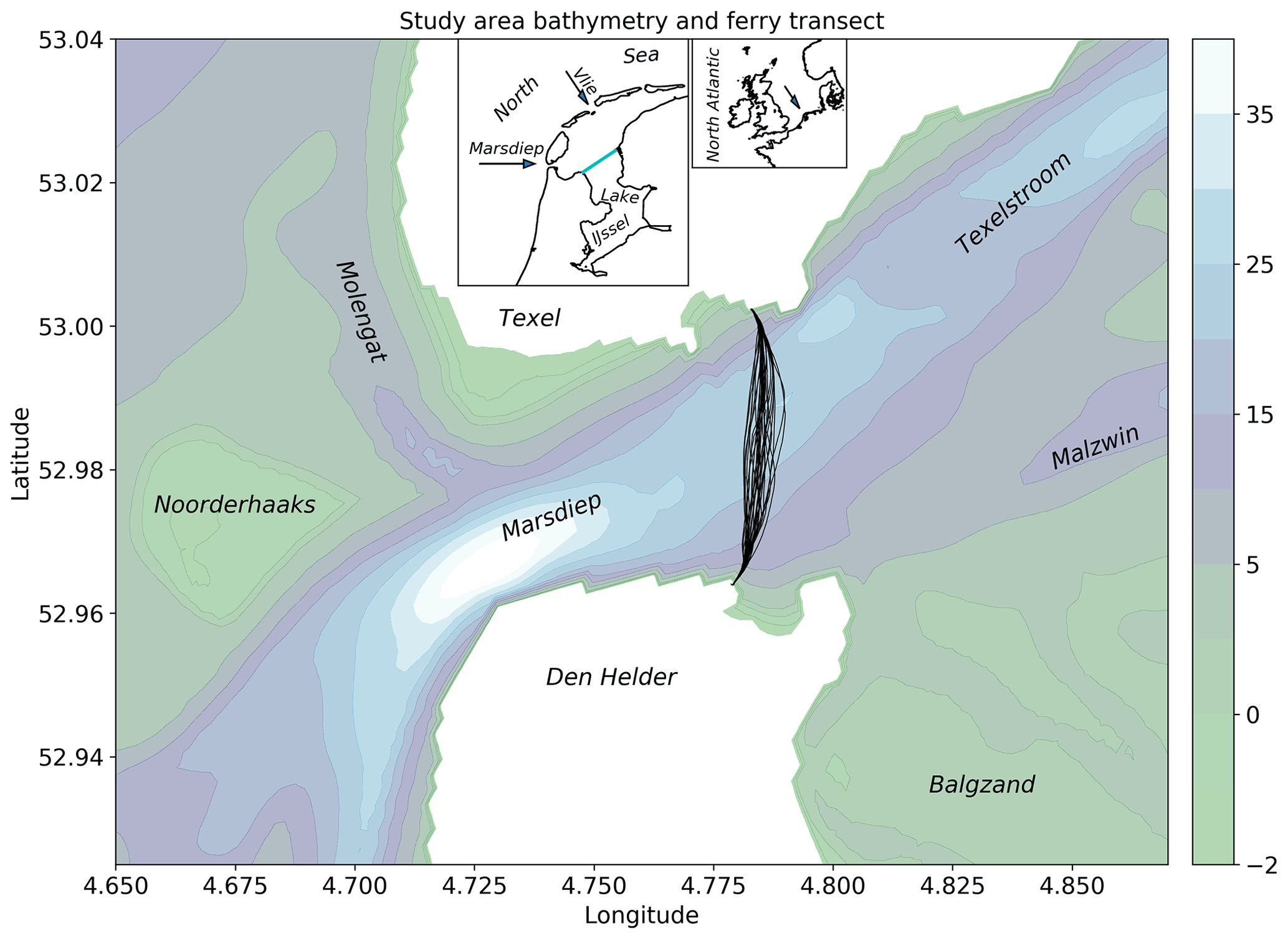
Figure 1Study area with a selection of ferry crossing trajectories. Contours are depths below mean sea level in metres. Insets: wider area with arrows pointing to the study area in the Marsdiep inlet and the Vlie inlet; the blue line is the closure dam Afsluitdijk.
The greatest depth of the Marsdiep is over 40 m, and the width is approximately 4 km. Tides in the Marsdiep are semi-diurnal, with a range of about 1.37 m (Nieuwhof and Vos, 2018). The tides are progressive in character, and tidal current speeds can reach 1.8 m3 s−1 and are strongly asymmetrical (Buijsman and Ridderinkhof, 2007). Fresh water is discharged into the western Wadden Sea through sluices, with a mean flux estimated at 450 m3 s−1 (Ridderinkhof, 1990); this can result in weak surface to bottom salinity gradients (Zimmerman, 1976a) and stratified conditions that carry internal waves (Groeskamp et al., 2011).
Residual currents are directed into the inlet in the southern part of the inlet and out of the inlet in the northern part, as a result of a suspected tidally driven residual eddy (Zimmerman, 1976b; Ridderinkhof, 1988). Tides are flood-dominant in the southern two-thirds and ebb-dominant in the northern one-third of the inlet in terms of peak velocity and tidal phase duration (Buijsman and Ridderinkhof, 2007). The tidal basin of the Marsdiep inlet has an average tidal prism of 0.99×10⁹ m3 with a standard deviation of 0.18×10⁹ m3 (Duran-Matute et al., 2014).
Table 1Previously reported residual volume fluxes through the Marsdiep inlet.
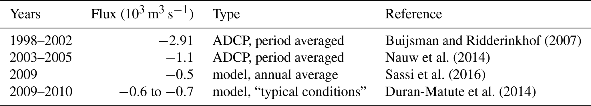
Volume transports at peak tidal currents are 5–10×104 m3 s−1 (Buijsman and Ridderinkhof, 2007; Nauw et al., 2014). Overall residual flows are from the Vlie inlet to the Marsdiep, and assumed to be driven by differences in tidal amplitudes and phases between the two inlets but display substantial wind-driven variability (Ridderinkhof, 1988; Buijsman and Ridderinkhof, 2007; Duran-Matute et al., 2014). As a result, reported residual flows through the Marsdiep vary, depending on the period considered (Table 1). Despite the generally outward direction of the residual flow, time lags and non-linearities ensure a residual import of suspended particulate matter (SPM) of 7–11 Mt yr−1 (Nauw et al., 2014).
The seabed morphology of the Marsdiep inlet is dominated by sand waves. In the northern half of the inlet, the sand waves are asymmetrical–trochoidal with heights and lengths of about 2 and 165 m, respectively and are subject to seasonal variations which may be related to temperature-driven changes in water viscosity, while in the southern half sand waves are progressive with heights and lengths of about 3 and 190 m, respectively (Buijsman and Ridderinkhof, 2008a, b). The sand waves migrate in the flood direction with speeds of up to 90 m yr−1. In the southern part, sand-wave migration and bedload transport are in the flood direction, and slightly more than half of the bedload transport is caused by tidal asymmetry, while the rest is caused by residual currents. In the northern part, sediment transport rates are opposite to the sand-wave migration direction suggesting that suspended load processes are dominant (Buijsman and Ridderinkhof, 2008b).
The tidal basin of the Marsdiep inlet was truncated by the damming of the Zuyderzee by the closure dam Afsluitdijk in 1932 (creating the current Lake IJssel), which caused a strong tidal and morphodynamic response. Although the morphology of the western Wadden Sea is still adjusting, the resulting import of sand has reduced to small values since 1980 (Elias et al., 2012; Wang et al., 2012) but with ongoing import of mud (Colina Alonso et al., 2021). The present small rates of sand import suggest that, in terms of volume, the system has reached a new dynamic equilibrium and is now mostly responding to other forcings such as climate change, sea-level rise and beach nourishments (Wang et al., 2012). Alongside these changes in the tidal basin, the ebb-tidal shoal Noorderhaaks has grown, and the seaward end of the inlet channel has shifted closer to the mainland coast (Elias et al., 2012), a process that is likely still ongoing.
2.1 ADCP observations
Two Teledyne RD Instruments Workhorse Monitor 1200 kHz ADCPs (http://www.teledynemarine.com/workhorse-monitor-adcp, last access: 8 December 2022) were mounted on the roll-on, roll-off ferry. One at each end of the ship, at 4.5 m below the sea surface. The ferry has identical bow and stern design and reverses sailing direction at each crossing (Fig. 1). In this configuration, one instrument is at the front of the ferry at any one time and undisturbed by the wake of the ship. Each instrument has four beams at angles of 20∘. Data were recorded in 50 bins of 0.5 m width. Further instrument settings are given in Table 2. In addition, both ends of the ferry were fitted with a differential GPS (JRC JLR-21/31), and a gyroscopic compass (Alphatron Alphaminicourse) to record position and orientation.

The ADCP, GPS and directional data were combined and stored by an on-board computer during the day and transmitted to a shore-based server when the ferry was in port at night. Recorded variables included navigational variables, water temperature, depth below the instrument for each beam, two orthogonal horizontal and one vertical velocity component for each bin, and signal attenuation along each beam for each bin. The horizontal velocities were converted to geo-referenced eastward and northward velocity components using the navigational data following the correction method for heading and tilt described by Joyce (1989); see also Buijsman and Ridderinkhof (2007). Water-depth and bin-depth measurements were automatically corrected by the instrument for variations in sound speed propagation using the instrument-mounted temperature sensor and a user-specified salinity of 28. Water depths were averaged over the four beams and corrected to depth below surface using the draught of the ship. The data also include the spike identification velocity (or “error velocity”) for each bin, which is a measure of the variation in the result when velocity is computed using different combinations of three of the four beams and is hence a measure for the reliability of the observations.
Typically, sailings started at 06:00, with an hourly outward-bound schedule from Texel and return journeys starting on the half hour from Den Helder (Fig. 1). Crossings typically took about 20 min. The last outward-bound sailing of the day started at 21:00, resulting in 32 single crossings per day. The sailing schedule was adjusted by the ferry operator in summer to account for daylight savings time. This schedule was maintained on most days of the year, with the exception of Christmas Day, New Year's Day, scheduled maintenance periods in January and November, and occasional unscheduled maintenance or extreme weather events (the latter typically occurs less than once a year). Occasionally, instrument failure also led to reduced data return. From March 2009 to July 2016 the ADCPs were mounted on the Dokter Wagemaker and from July 2016 to present on the Texelstroom. The setup on the Dokter Wagemaker was configured similarly to that described above but with a single GPS midships (Furuno SC110, https://www.furunousa.com/en/products/sc110, last access: 8 December 2022) and a single gyroscopic compass included in the GPS.
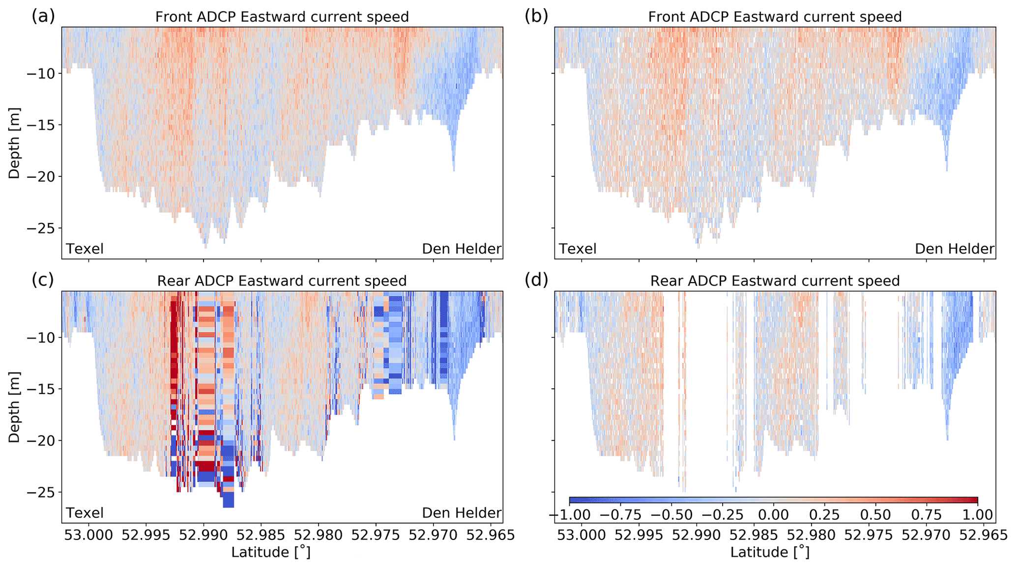
Figure 2Example of QA procedure, 7 April 2021, 06:00 departure, sailing from Texel to Den Helder. (a) Original and (b) “good” and “probably good” data for the front ADCP. Panels (c) and (d) show the same for the rear ADCP. Velocities in m s−1. The direction of view is in the eastward or flood direction.
2.2 Data processing
2.2.1 Quality assessment
Quality flags were added to the depth-resolved variables using a threshold value for the spike identification velocity. For the values of the quality assessment (QA) flags, we used designations defined by SeaDataNet (49 = good value; 50 = probably good value; 52 = bad value; https://www.seadatanet.org/Standards/Data-Quality-Control, last access: 8 December 2022). To define the threshold values, we inspected transects recorded by the ADCP mounted on the rear of the ship. Such records contain clearly visible anomalous velocities when the ADCP signal is disturbed by the wake of the thrusters of the ship. Such wake-affected velocities were adequately identified using a spike identification velocity threshold of 0.15 m s−1 and nearly always for a spike identification velocity threshold of 0.2 m s−1. Hence, data points corresponding to a spike identification velocity threshold of less than 0.15 m s−1 were flagged as “good value”, between 0.15 and 0.2 m s−1 as “probably good value”, and those greater than 0.2 m s−1 as “bad value”. As such disturbances in the observations tended to extend throughout the water column, all bins in the vertical at locations with more than 30 % bad values were flagged as bad value. The same thresholds were assumed to hold for the ADCP mounted on the front of the ship and seem appropriate as it allows for errors of up to about 15 % of typical maximum currents. This choice is, however, somewhat subjective, and other threshold values could be set for different applications, e.g. when individual transects are studied. In the remainder of this paper, both good values and probably good values were included.
2.2.2 Latitudinal gridding of each crossing
Because of variations in the speed of the ferry, different crossings resulted in varying amounts of data with a location-dependent data density. Moreover, as the data from both front and rear ADCPs typically contain QA-related gaps, not a single crossing resulted in continuous coverage of the cross section. To obtain regular data, use the results of both ADCPs and obtain maximum coverage, each transect was subdivided into 100 equidistant latitudinal intervals of 42.74 m, while retaining the longitudinal positions and vertical gridding. The data from both ADCPs were collected in each resulting latitude–depth grid cell and averaged. For each latitude–depth grid cell, a standard deviation was calculated to provide an uncertainty estimate for the mean value of each grid cell. Water depths were similarly averaged per latitudinal grid interval. These data were used to calculate cross-sectionally aggregated averages and trends (Sect. 2.2.3). To calculate cross-sectionally resolved patterns (Sect. 2.2.4), similar gridding was carried out but after first projecting each observed column of the curved transect onto a straight central north–south transect subdivided into the same latitudinal intervals. This projection was carried out by moving each column in the opposite direction of the current measured at the surface until it met the straight central transect. Resulting data on the central transect were averaged for each latitudinal interval.
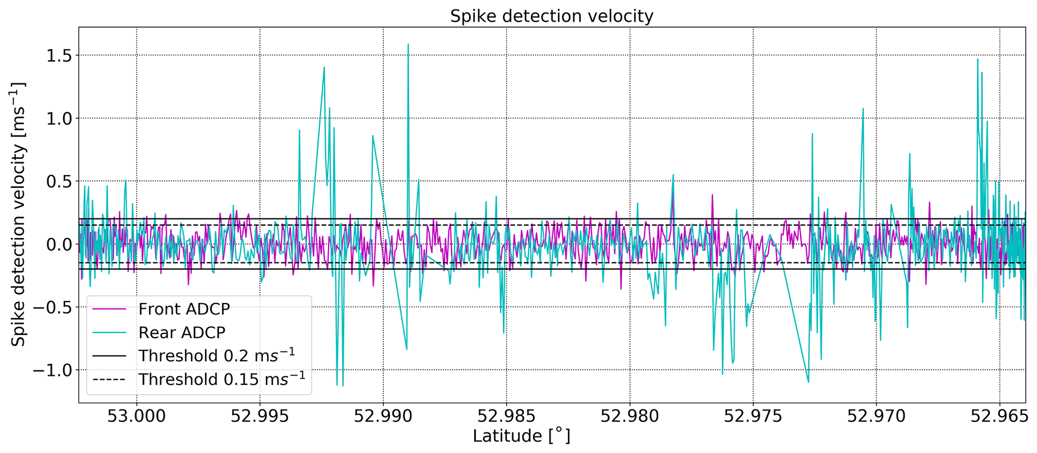
Figure 3Example of spike detection velocity compared to QA thresholds; second bin below the vessel, 7 April 2021, 06:00 departure.
2.2.3 Time series and trends of cross-sectionally aggregated depths and flows
Cross-sectionally averaged depths and eastward cross-sectionally integrated volume fluxes were calculated for each latitudinally gridded crossing to construct time series to analyse for decadal trends.
Cross-sectionally averaged depths contain some variation related to longitudinal position and associated seabed morphology (e.g. Buijsman and Ridderinkhof, 2008a, b), but these will only contribute to the uncertainty of the trend estimates (see below) and not introduce a bias. Cross-sectionally averaged depths were calculated by averaging over the latitudinal grid intervals. Annual mean depth profiles along the cross section were also plotted to illustrate the temporal changes.
As the transects cover the entire cross section and both ends of the transects have nearly identical longitudinal coordinates (resulting in only a net north–south displacement of the ship for each crossing), eastward cross-sectionally integrated volume fluxes represent the full volume flux through the Marsdiep. Eastward cross-sectionally integrated volume fluxes were calculated by multiplying the eastward flow velocities by the surface area of each cross-sectional grid cell and then adding all cross-sectional grid cells. To include an estimate of the volume flux between the water surface and the first bin measured by the ADCP below the ferry, the value of the first bin was first copied to equally sized bins covering that gap.
Tidal harmonic analysis (Doodson, 1921) was applied to the time series as a whole, estimating the amplitudes of the 21 main tidal constituents, including nodal corrections, their Greenwich phase and the mean residual component. The time series was also split up into yearly intervals, with tidal harmonic analysis applied to each individual year. Buijsman and Ridderinkhof (2007) established that the largest 15 constituents represent 96 % of the tidal variance. Yearly intervals were used to enable the detection of trends in harmonic constituents and to facilitate comparison of the yearly mean residual volume fluxes to earlier estimates. To obtain trends in the residual cross-sectional depth changes and volume fluxes, the time series as a whole were de-tided by subtracting a tidal time series reconstructed from the harmonic analyses. Decadal trends were calculated for the de-tided time series as the slope of a straight line estimated using a least-squares fit. To estimate trends in the tidal harmonic constituents, regression lines were fitted through the yearly amplitudes and phases. Here, we only present and discuss variables with an estimated slope that exceeds 2 times the standard error of the fit (corresponding to a 95 % confidence interval).
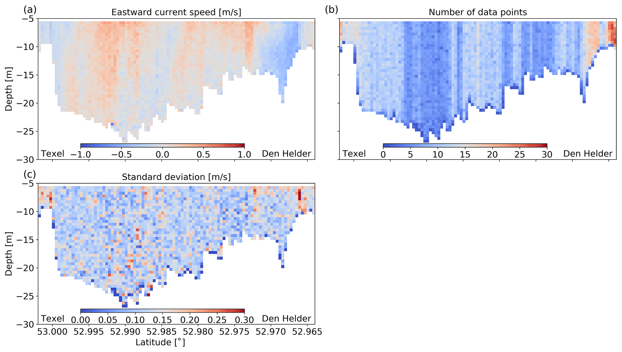
Figure 4Example of transect based on latitudinally gridded, quality-assured data from front and rear ADCP (Fig. 2b, d), 7 April 2021, 06:00 departure. (a) Resulting mean gridded eastward current speed; (b) number of data points per grid cell; (c) standard deviation per grid cell. The direction of view is in the eastward or flood direction.
To test the hypothesis (Ridderinkhof, 1988; Buijsman and Ridderinkhof, 2007; Duran-Matute et al., 2014) that the variations in residual flow are mainly wind-driven, a scatter plot was constructed of the annual residual transports as a function of the annual mean eastward wind-speed component derived from the ECMWF ERA5 reanalysis (C3S, 2019).
2.2.4 Cross-sectionally resolved temporal mean patterns and trends
To calculate cross-sectionally resolved temporal mean patterns and trends, the latitudinally gridded data were first corrected for water-level changes such as tides using the bed level of the first couple of latitudinal grid intervals of the transect on the Texel side as a reference. Then, annual and decadal means and trends were calculated for the residual velocity components for each latitude–depth grid cell in the same way as for the transports: by performing a harmonic analysis, de-tiding the time series and calculating a linear least-squares fit through the residuals. To present the results, contour plots of the residual velocities and trends as well as line graphs of the depth- and cross-sectionally averaged residual velocities were constructed.
3.1 Example of quality assessment
As an example of the QA procedure, eastward velocities measured on the transect sailed on 7 April 2021, 06:00 local time, are given (Fig. 2). The left two panels show the uncorrected eastward velocities for the front (a) and rear (c) ADCP, and the panels on the right (b, d) the corresponding quality-assured velocities. In Fig. 2c, the data affected by the ship's propulsion system are clearly visible and were effectively removed in Fig. 2d. The QA procedure also removed some data from the front ADCP (Fig. 2b). To further illustrate the procedure, the spike identification velocity for the second ADCP bin of both instruments was plotted along the transect, including the thresholds (Fig. 3).
3.2 Example of latitudinal gridding
An illustration of the latitudinal gridding of the quality-assured data of both ADCPs, combined for the same date and time shows a coherent profile without data gaps (Fig. 4a). Despite strong variation in the number of data points per grid cell (Fig. 4b) due to a combination of changes in vessel speed and gaps in the quality-assured data (Fig. 2), standard deviations showed no obvious pattern over the cross section (Fig. 4c) (except near the bottom as the two ADCPs, which are a ship's distance apart, may follow slightly different trajectories and encounter different seabed topography), suggesting uniform quality of the eastward current speeds constructed in this way for the cross section.
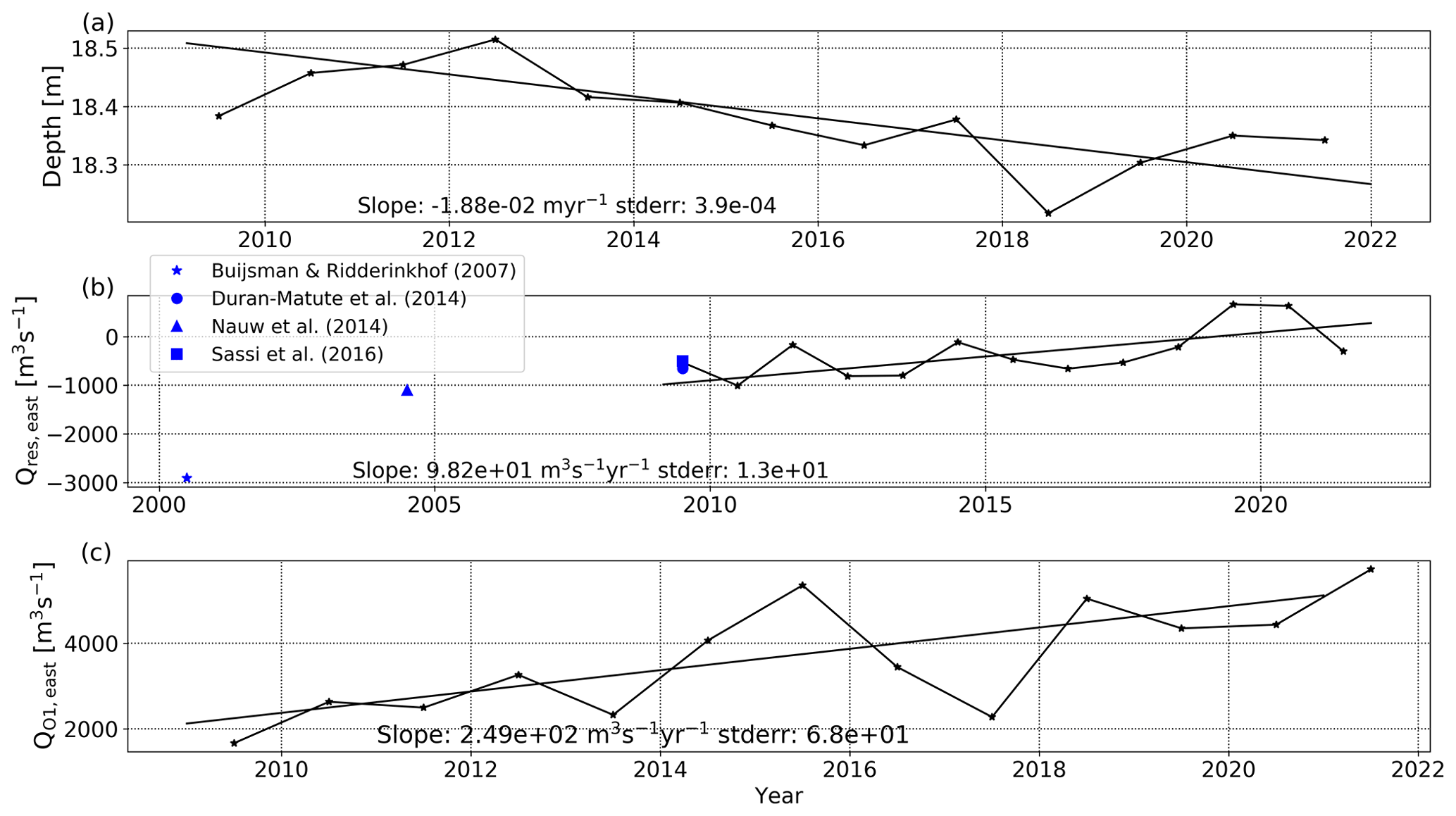
Figure 5Observed trends after applying harmonic analysis. (a) Annual residual cross-sectionally averaged depth; trend line based on the de-tided time series. (b) Annual residual cross-sectionally integrated eastward volume flux including values reported earlier; trend line based on the de-tided time series. (c) Annual O1 lunar diurnal constituent amplitude of cross-sectionally integrated eastward volume flux; trend line based on the annual amplitudes.
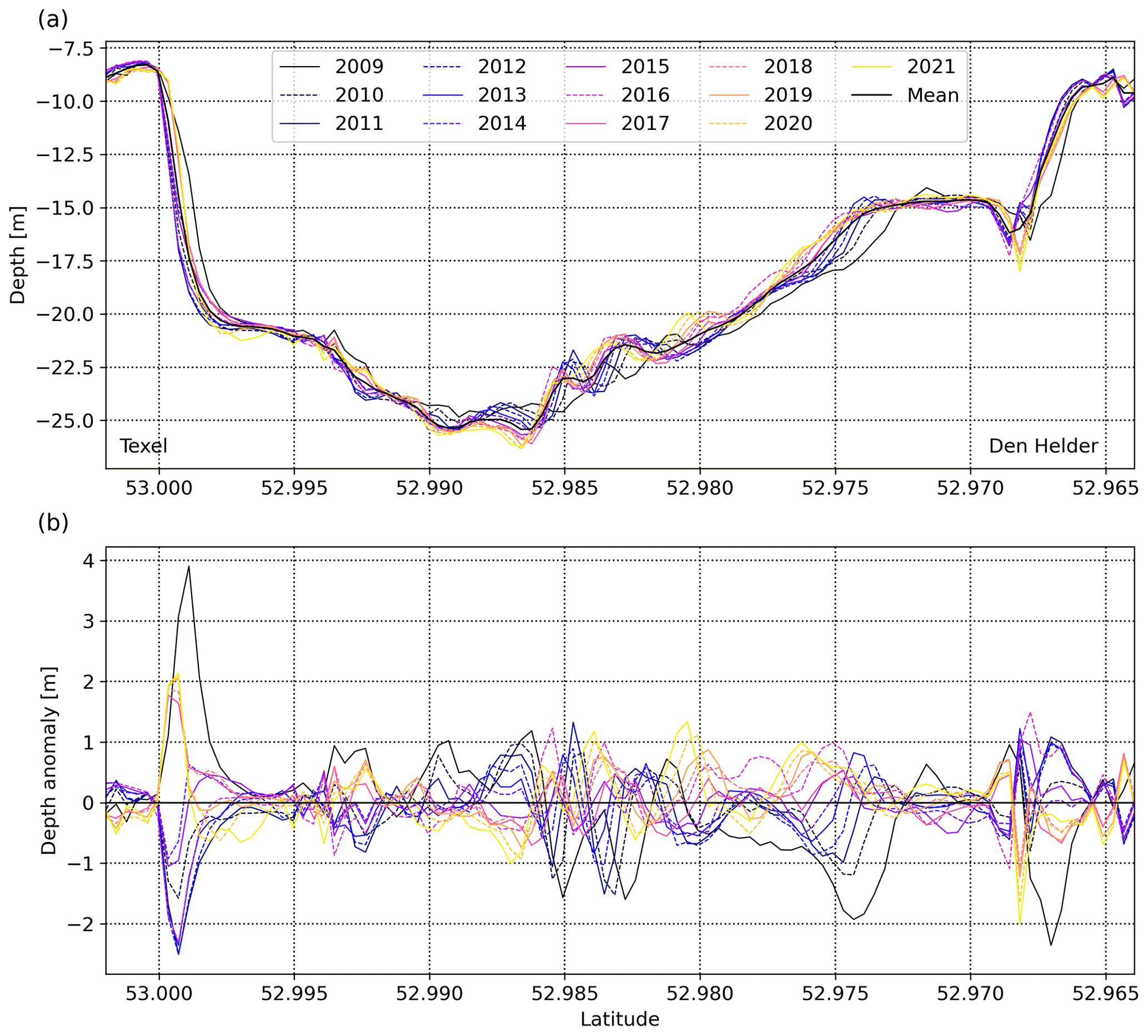
Figure 6(a) Annual averaged depths along the transect and (b) the annual depth anomaly with respect to the 13-year mean.
3.3 Time series of cross-sectionally aggregated averages and trends
Time series of cross-sectionally averaged depth (Fig. 5a) showed an average of 18.4 m and a shoaling trend of 1.88 cm yr−1 with a standard error of 0.04 cm yr−1. Similarly, the cross-sectionally integrated volume flux (Fig. 5b) showed an average outflow that changed from around 1000 m3 s−1 in 2009 to around 0 in recent years, with a reducing trend of 98 m3 s−1 yr−1 and a standard error of 13 m3 s−1 yr−1, which continued compared with values reported for earlier years. Most notably, the volume flux has been transitioning to positive values (net inflow) in recent years. Finally, the amplitude of the O1 tidal constituent of the volume flux (Fig. 5c) more than doubled in the period considered, with a trend of 249 m3 s−1 yr−1 and a standard error of 68 m3 s−1 yr−1. This was the only tidal constituent in the ADCP data with a consistent trend exceeding 2 times the standard error.
Plotting the annual residual eastward volume fluxes as a function of the annual mean eastward wind-speed component did not suggest an evident correlation (not shown).

Figure 7Long-term mean horizontal velocities in the east (a) and north (b) direction and their respective trends (c, d). In (a) red indicates an inflow (flood). Levels near the surface subject to vertical tidal changes were excluded. The direction of view is in the eastward or flood direction.
The annually averaged depths along the transect (Fig. 6) revealed the infilling of a substantial depression in the southern flank of the inlet around 52.975∘ N as well as an increase in the maximum depth along the transect between 52.990∘ N and 52.985∘ N but no major changes in the cross-sectional geometry. The apparent shift in the flank of the channel near Texel after 2017 coincides with the change-over of the instrumentation from the Dokter Wagemaker to the Texelstroom, and is likely an artefact, potentially related to a slight change in approach route related to differences in the handling of the ships, which differ considerably in size. Note that the profile of 2009 is less reliable than the others as only data from the later part of the year were available.
3.4 Cross-sectionally resolved temporal mean patterns and trends
The 13-year residual eastward velocities showed outflow in the northern part of the inlet, with the highest values close to the coast of Texel in the upper part of the water column and inflow in the southern part of the inlet, with higher values in the lower part of the water column (Fig. 7a). Both inflow and outflow appear to consist of two kernels. The trends in the residual eastward velocity show a vertically banded structure of alternating increases and decreases, with the strongest band in the southern part of the inlet (Fig. 7c). A striking feature was a strongly negative trend near the bottom in the southern part of the inlet, likely related to the local shoaling (Fig. 6). Standard errors of the trend estimates were small, except near the surface and the bottom, where it increased to 0.002 m s−1yr−1 due to the fluctuating water levels and where local variations in depth associated with individual transects and morphodynamic changes affect the estimates. As a result, the near-surface and near-bottom trend estimates have a high level of uncertainty.
The northward velocities were positive near the surface in the southern part of the inlet and near the bottom in the northern part of the inlet (Fig. 7b). They were negative elsewhere, with the weakest negative values in the central part of the inlet. This pattern suggests a double gyre in the plane of the transect, but this could not be confirmed as the vertical velocities recorded by the ADCPs were affected by the flow induced by the forward motion of the ship. The trends in the northward velocity reflected the vertically banded structure of the trends in the eastward velocities but also indicated a weakening of both the positive and negative residual velocities, suggesting a weakening of the suspected double-gyre pattern (Fig. 7d). The standard errors of the trend estimates were similar to those of the eastward velocity.
Depth- and cross-section averages of the residual eastward velocities provide another way of presenting the main patterns and also allow for a depiction of the interannual variations. The depth averages of the 13-year residuals again showed the outflow in the northern part and the inflow in the southern part (Fig. 8a, thick black line). The individual years clustered relatively close to this line, with the largest variations near the maximum residual inflow in the southern part of the inlet. The cross-sectionally averaged values of the 13-year residual eastward velocity showed outflow in the top 10 m of the water column and inflow in the 15 m below that (Fig. 8b, thick black line), suggesting a component of estuarine circulation to the flow. Interannual variations were largest for the outflow velocities.
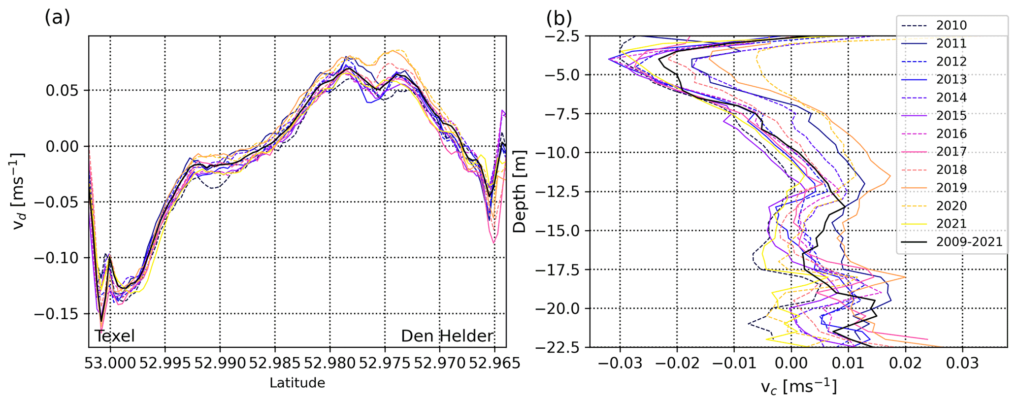
Figure 8(a) Depth-averaged eastward residual velocities along the transect and (b) cross-sectionally averaged eastward residual velocities as a function of depth for each year and for the whole time series.
4.1 Cross-sectionally resolved residual flow patterns and trends
The overall cross-sectional pattern of inflow in the southern part of the inlet and outflow in the northern part of the inlet, with a weak estuarine circulation component in the vertical corresponds with the results of earlier investigations (Zimmerman, 1976a, b; Ridderinkhof, 1988; Buijsman and Ridderinkhof, 2007). Huijts et al. (2009) used a semi-analytical model of a schematised curved tidal channel to investigate the cross-sectional patterns of residual flows in the stream-wise and cross-channel directions caused by tidal rectification, along-channel density gradients, along-channel winds and river discharge. Their pattern for streamwise residual flow induced by tidal rectification corresponds well with the pattern of eastward residual flow in the Marsdiep, including the double inflow–outflow kernels, which only occur for the tidal rectification component. Their pattern for cross-channel residual flow by tidal rectification shows a double-gyre pattern like that of the northward residual currents in the Marsdiep but with reversed direction. The causes of this difference are not immediately clear, but the geometry of the Marsdiep (Fig. 1) is much more complex than the schematised curved channel in the model of Huijts et al. (2009): (i) the main channel is not aligned with the coasts and the angle is different at either side; (ii) just seaward of the transect, the main channel curves in the other direction, and on the basin side the main channel is more or less straight. Moreover, the ferry transect slants across the main channel at a fairly large angle, the exact value of which is difficult to estimate because of these changes in curvature. The direction of the gyre pattern corresponds with that observed by Nunes and Simpson (1985) during the flood phase of the tide in an estuary in Wales (UK) and explained by strong friction with the sides of the channel. Cui et al. (2018) also observed this pattern in an estuary in the Gulf of Mexico, where they also observed the reverse pattern during the ebb phase. So it is possible that, in a flood-dominant estuary like the Marsdiep, the flood-phase pattern is expressed in the long-term mean as we see in the observations presented here. As Huijts et al. (2009) used a purely sinusoidal tide superimposed on a river runoff, effectively creating ebb dominance in terms of residual flow and peak velocities in their model, this reasoning may explain the discrepancy if this effect dominates over the influence of geometric differences. Hence, the correspondence of the observed eastward residual flow pattern with the modelled streamwise residual flow pattern induced by tidal rectification is a strong indication that this mechanism is dominant in shaping the cross-sectional residual flow patterns in the Marsdiep.
The trends in the cross-sectional residual flow pattern suggest a slight intensification of both the outflow in the northern part of the inlet and of the inflow in the southern part of the inlet, in particular in later years, with the inflow increasing more than the outflow. There was also a weakening of the double-gyre pattern in the cross section. Moreover, there were slight latitudinal shifts in the double-kernel pattern, but these do not seem to have a systematic direction. There was also a local response to the infilling of a depression at 52.975∘ N. These trends suggest changes in the tidal rectification and frictional processes, possibly related to larger-scale morphodynamic changes such as the ongoing infilling, sea-level rise, and channel migration in the Wadden Sea and in the ebb-tidal delta (Wang et al., 2012; Elias et al., 2012). Slight changes in tides may also be involved, as is suggested by the observed trends in O1 currents and flows. These could be related to bathymetric changes (Benninghoff and Winter, 2019; Jacob and Stanev, 2021; Colina Alonso et al., 2021) and/or sea-level rise (Wachler et al, 2020) that may alter the resonance characteristics of the basin. Larger-scale changes in tides in the North Sea likely also play a role: these resulted in small increases in tidal range near the Marsdiep from 2010–2015 but also in differences in trends in tidal range between the Marsdiep and the Vlie inlets between 1958 and 2014 (Jänicke et al., 2021). Jänicke et al. (2021) identify two components driving the changes in tides in the North Sea: a large-scale barotropic component that involves the north Atlantic Ocean and a regional baroclinic component that relates to stronger stratification in the southern North Sea. It is not clear why the O1 component of the flow changes significantly, while the ADCP data could not detect significant changes in other constituents. Tide gauge data most likely offer a more accurate way to analyse trends in tides in the study area than the ADCP data analysed here as they are more accurate, have higher sampling frequency, measure continuously and cover a wider area. However, such a study is beyond the scope of this paper.
4.2 Trends in cross-sectionally aggregated residual flows
We found a significant trend in the cross-sectionally aggregated residual flow in the Marsdiep tidal inlet, suggesting an imminent reversal from net outflow to net inflow. Four processes can contribute to such changes: changes in wind climate, changes in freshwater input, morphodynamic changes and changes in tidal forcing.
We established that wind forcing, suggested in earlier studies to influence residual flows (Buijsman and Ridderinkhof, 2007; Duran-Matute et al., 2014), is not correlated to the trend observed in the ADCP data. Hence, even though wind and storms may affect the flow on timescales of days to weeks, we do not think that this process is primarily responsible for the observed reduction in residual flow on interannual timescales.
Discharge of fresh water into the western Wadden Sea was estimated to be 450 m3 s−1 on average (Ridderinkhof, 1990), much less than the historic residual outflow (Table 1). Also, freshwater discharge cannot reverse in direction. Thus, this process is not primarily responsible for the observed reduction in residual flow either.
Because the western Wadden Sea has reached near-equilibrium following the construction of the closure dam (Elias et al., 2012.), ongoing morphodynamic changes within the western Wadden Sea are likely dominated by relatively local, internal dynamics. Hence, it seems unlikely that the current morphodynamic processes are the main driver for the changes in residual flow. However, further work would be needed to confirm this.
Ridderinkhof (1988) showed that the outflow at that time was related to a residual circulation entering through the Vlie inlet and driven by differences in amplitudes and phases of the tides between the two inlets. Hence, we hypothesise that the main process driving the trend in residual flows is the baroclinically derived change in the difference in tides between the Marsdiep and Vlie inlets caused by climate change identified by Jänicke et al. (2021). As a result, with warming trends expected to continue, we expect a permanent reversal of the residual flow followed by a strengthening net inflow to occur in the next decade(s). Similar changes may happen in other multiple inlet systems bordering temperature-stratified seas elsewhere in the world.
4.3 Potential consequences of a reversal in residual flow
The reversal of the residual flow in the Marsdiep will be linked with a reversal and potential changes in the residual flow patterns in the western Wadden Sea. This may influence physical factors such as temperature and salinity distributions and may also increase the import of fine suspended sediment through the Marsdiep inlet, while reducing that through the Vlie inlet. Moreover, it may change pathways of nutrient supply and transport of passive propagules (eggs and early stage larvae of marine organisms). Such changes may cascade up through the Wadden Sea ecosystem, that is already influenced by anthropogenic pressures and more direct effects of climate change. However, as the residual flows are much smaller than the tidal flows and even heterogeneous within the Marsdiep inlet itself, it is not possible to infer such effects from this study and further work is needed.
4.4 Suggestions for further research
Further work is needed to fully understand the causes, significance and effects of the reversal of the residual flow in this multi-inlet tidal embayment. Next steps could include detailed analysis of the local tide gauge data to refine our understanding of the driving forces, model projections of climate-driven trends in North Sea tides, model studies detailing the processes driving the residual circulation in the Wadden Sea and projecting future changes as well as implications for the regional sediment budget, and model studies projecting changes in the ecosystem in response. Existing observations of ecosystem variables and components should be examined, and wider observational campaigns could be initiated to gain further understanding, underpin models and observe predicted effects.
The TESO ADCP data are available on request.
JvdM designed the study, processed the data, carried out the analysis and interpretation, and wrote the paper. LRMM and SG contributed to several revisions.
The contact author has declared that none of the authors has any competing interests.
Publisher’s note: Copernicus Publications remains neutral with regard to jurisdictional claims in published maps and institutional affiliations.
Many people contributed to collecting the TESO ADCP time series data, a collaborative effort of the Royal Netherlands Institute for Sea Research (NIOZ) and the Royal TESO N.V. ferry company for more than 2 decades, and we want to extend our thanks to them, although not all can be named. Herman Ridderinkhof initiated the observations. Frans Eijgenraam and Eric Wagemaakers developed, installed and maintained the adaptations to the ferries, the instrumentation and the software. Numerous MSc students, PhD students and postdocs have worked on the data, and some of their papers are referenced here. In recent years, Erin Lejeune and Mariana de Botton, both funded through Utrecht University–NIOZ work experience placements, worked on modernising the automated data postprocessing that made this paper possible.
This research has been supported in part by Utrecht University.
This paper was edited by Markus Meier and reviewed by Zheng Bing Wang and Johannes Becherer.
Benninghoff, M. and Winter, C.: Recent morphologic evolution of the German Wadden Sea, Sci. Rep., 9, 9293, https://doi.org/10.1038/s41598-019-45683-1, 2019.
Buijsman, M. C. and Ridderinkhof, H.: Long-term ferry-ADCP observations of tidal currents in the Marsdiep inlet, J. Sea Res., 57, 237–256, https://doi.org/10.1016/j.seares.2006.11.004, 2007.
Buijsman, M. C. and Ridderinkhof, H.: Long-term evolution of sand waves in the Marsdiep inlet, I: High-resolution observations, Cont. Shelf Res., 28, 1190–1201, 2008a.
Buijsman, M. C. and Ridderinkhof, H.: Long-term evolution of sand waves in the Marsdiep inlet, II: Relation to hydrodynamics, Cont. Shelf Res., 28, 1202–1215, 2008b.
Colina Alonso, A., van Maren, D. S., Elias, E. P. L., Holthuijsen, S. J., and Wang, Z. B.: The contribution of sand and mud to infilling of tidal basins in response to a closure dam, Mar. Geol., 439, 106544, https://doi.org/10.1016/j.margeo.2021.106544, 2021
Copernicus Climate Change Service (C3S): ERA5: Fifth generation of ECMWF atmospheric reanalyses of the global climate, Copernicus Climate Change Service Climate Data Store (CDS), March 2019, https://cds.climate.copernicus.eu/cdsapp#!/home (last access 9 December 2022), 2019.
Cui, L., Huang, H., Li, C., and Justic, D.: Lateral circulation in a partially stratified tidal inlet, J. Mar. Sci. Eng., 6, 159, https://doi.org/10.3390/jmse6040159, 2018.
Doodson, A. T.: Harmonic Development of the Tide-Generating Potential, P. Roy. Soc. A, 100, 305–329, https://doi.org/10.1098/rspa.1921.0088, 1921.
Duran-Matute, M., Gerkema, T., de Boer, G. J., Nauw, J. J., and Gräwe, U.: Residual circulation and freshwater transport in the Dutch Wadden Sea: a numerical modelling study, Ocean Sci., 10, 611–632, https://doi.org/10.5194/os-10-611-2014, 2014.
Elias, E. P. L., van der Spek, A. J. F., Wang, Z. B., and de Ronde, J.: Morphodynamic development and sediment budget of the Dutch Wadden Sea over the last century, Neth. J. Geosci., 91, 293–310, 2012.
Groeskamp, S., Nauw, J. J., and Maas, L. R. M.: Observations of estuarine circulation and solitary internal waves in a highly energetic tidal channel, Ocean Dyn., 61, 1767–1782, https://doi.org/10.1007/s10236-011-0455-y, 2011.
Jacob, B. and Stanev, E. V.: Understanding the Impact of Bathymetric Changes in the German Bight on Coastal Hydrodynamics: One Step Toward Realistic Morphodynamic Modeling, Front. Mar. Sci., 8, 640214, https://doi.org/10.3389/fmars.2021.640214, 2021.
Jänicke, L., Ebener, A., Dangendorf, S., Arns, A., Schindelegger, M., Niehüser, S., Haigh, I. D., Woodworth, P., and Jansen, J.: Assessment of tidal range changes in the North Sea from 1958 to 2014, J. Geophys. Res.-Oceans, 126, e2020JC016456, https://doi.org/10.1029/2020JC016456, 2021.
Joyce, T. M.: On in situ “calibration” of shipboard ADCPs, J. Atmos. Ocean. Technol., 6, 169–172, 1989.
Nauw, J. J., Merckelbach, L. M., Ridderinkhof, H., and van Aken, H. M.: Long-term ferry-based observations of the suspended sediment fluxes through the Marsdiep inlet using acoustic Doppler current profilers, J. Sea Res., 87, 17–29, https://doi.org/10.1016/j.seares.2013.11.013, 2014.
Nieuwhof, A. and Vos, P.: New data from terp excavations on sea-level index points and salt marsh sedimentation rates in the eastern part of the Dutch Wadden Sea, Neth. J. Geosci., 97, 31–43, https://doi.org/10.1017/njg.2018.2, 2018.
Nunes, R. A. and Simpson, J. H.: Axial convergence in a well-mixed estuary, Eastuar. Coast. Shelf S., 20, 637–649, 1985.
Ridderinkhof, H.: Tidal and residual flows in the western Dutch Wadden Sea I: numerical model results, Neth. J. Sea Res., 22, 1–21, 1988.
Ridderinkhof, H.: Residual currents and mixing in the Wadden Sea, PhD thesis, Rijksuniversiteit Utrecht, Utrecht, 1990.
Sassi, M. G., Gerkema, T., Duran-Matute, M., and Nauw, J. J.: Residual water transport in the Marsdiep tidal inlet inferred from observations and a numerical model, J. Mar. Res., 74, 21–42, 2016.
Wachler, B., Seiffert, R., Rasquin, C., and Kösters, F.: Tidal response to sea level rise and bathymetric changes in the German Wadden Sea, Ocean Dyn., 70, 1033–1052, https://doi.org/10.1007/s10236-020-01383-3, 2020.
Wang, Z. B., Hoekstra, P., Burchard, H., Ridderinkhof, H., de Swart, H. E., and Stive, M. J. F.: Morphodynamics of the Wadden Sea and its barrier island system, Ocean Coast. Man., 68, 39–57, 2012.
Zimmerman, J. T. F.: Mixing and flushing of tidal embayments in the western Dutch Wadden Sea part I: Distribution of salinity and calculation of mixing time scales, Neth. J. Sea Res., 10, 149–191, 1976a.
Zimmerman, J. T. F.: Mixing and flushing of tidal embayments in the western Dutch Wadden Sea part II: Analysis of mixing processes, Neth. J. Sea Res., 10, 397–439, 1976b.