Accuracy of numerical wave model results: application to the Atlantic coasts of Europe

Numerical wave models are generally less accurate in the coastal ocean than offshore. It is generally suspected that a number of factors specific to coastal environments can be blamed for these larger model errors: complex shoreline and topography, relatively short fetches, combination of remote swells and local wind seas, less accurate wind fields, presence of strong currents, bottom friction, etc. These factors generally have strong local variations, making it all the more difficult to adapt a particular model setup from one area to another. Here we investigate a wide range of modeling choices including forcing fields, spectral resolution, and parameterizations of physical processes in a regional model that covers most of the Atlantic and North Sea coasts. The effects of these choices on the model results are analyzed with buoy spectral data and wave parameter time series. Additionally, satellite altimeter data are employed to provide a more complete performance assessment of the modeled wave heights as a function of the distance to the coast and to identify areas where wave propagation is influenced by bottom friction. We show that the accurate propagation of waves from offshore is probably the most important factor on exposed shorelines, while other specific effects can be important locally, including winds, currents, and bottom friction.

1 Introduction

Numerical wave models have been used from the global ocean to the coast, for a wide range of applications, including the design and safe operation of seagoing structures such as ships, platforms, and wind turbines. The progressive improvement in parameterizations in spectral wave models based on the wave action equation, like SWAN (Booij et al., 1999) or WAVEWATCH III^® (The WAVEWATCH III® Development Group, 2019) (WW3), has helped to continuously extend their use into coastal regions and areas with shallower water depths. With the introduction of currents, bottom friction related to different sediment types, and coastal reflection, errors in the main wave parameters have dropped to levels similar to open-ocean simulations (Ardhuin et al., 2012; Roland and Ardhuin, 2014; Salmon et al., 2015). High-resolution modeling has also become more efficient with the implementation of unstructured grids (mesh), providing flexible spatial resolution taking into account wave characteristics and bathymetry features (Benoit et al., 1996; Roland, 2008; Dietrich et al., 2011; Alves et al., 2013). In particular, previous works by Boudière et al. (2013) and Wu et al. (2020) present the implementation and validation of high-resolution hindcasts for wave resource assessments along French waters and the US west coast, respectively.

In general, the accuracy of spectral models is a function of at least three main factors: first, the accuracy of forcing fields (e.g., Cavaleri and Bertotti, 1997); second, the realism of the parameterization of processes representing spectral wave evolution (e.g., Ardhuin et al., 2010); and third, discretization and numerical schemes (e.g., Tolman, 1995a; Roland and Ardhuin, 2014). For example, in the hindcast presented in Alday et al. (2021), more accurate wave height distributions were obtained at a global scale by adjusting parameterizations and discretizations. When it comes to nested models, the characteristics of the boundary conditions should also be taken into account.

In the present paper the analysis is extended to intermediate and shallow-water depths. To this end, we present a high-resolution wave hindcast for European Atlantic waters, using boundary conditions from Alday et al. (2021). Throughout the study we attempt to determine which elements in the model setup have a significant effect on the characteristics of the simulated sea states and hence the accuracy of the results. Given the wide range of bathymetry features, bottom sediment types, fetch, and tidal amplitudes in coastal environments, we also verify when and where these choices introduce important changes.

Particular attention is paid to the effects of tidal currents, directional resolution, and bottom friction over the simulated wave fields. Performance analysis of the results is conducted in terms of the significant wave heights, directional spreading, peak direction, and mean periods. Additionally, analyses on the energy distribution as a function of frequency were conducted to further explore the changes introduced through modifications in the forcing, resolution, or the boundary conditions.

Details on the model setup, source terms, and numerical choices are presented in Sect. 2. Wave measurements used for sensitivity analyses and validation are given in Sect. 3. The model performance analysis is described in Sects. 4 and 5, followed by its validation and conclusions in Sects. 6 and 7.

2 Model setup and sensitivity tests

2.1 Mesh construction

The triangle grid used for the simulations was created using an interface developed at BGS IT&E. The main data sources employed for the mesh construction were coastline polygons from OpenStreetMap (last update of the dataset used: 10 June 2018, 09:33 UTC), bathymetric information from EMODnet (2016 version), and HOMONIM (Historique Observation MOdélisation des NIveaux Marins) digital terrain models. These data have gridded resolutions of ∼210 and ∼110 m, respectively, with depths defined with respect to the mean sea level. Although the coastline is generally located at high water levels with an exact definition that varies from country to country, we have chosen to impose a constant 2 m minimum depth value at the coastline to preserve the shoreline geometry and avoid unrealistic wave height gradients at the nearshore that could be triggered by the combination of large tidal sea level variations (wet and dry effect) with inadequate spatial resolution in very shallow areas close to the shore.

Previous to the triangulation, a node homogenization of the coastlines was applied to ensure a minimum segment length of 400 m in the polygons. An extra segment coarsening (up to 1200 m) and trimming was applied along the Norwegian fjords to reduce the final number of nodes. This coarsening allowed a lower Courant–Friedrichs–Lewy (CFL) number, which makes it possible to use a larger time step for wave propagation (13 s in this case for our lowest frequencies), but it also implies that details of the Norwegian coastline are not as well resolved. In addition, nodes from an existing mesh (Boudière et al., 2013) with the exception of those placed less than 800 m from the coastlines, were included in the generation of the new mesh fixing their previous position. This was done to facilitate the use of the new results by users of the previous hindcast.

Finally, the resolution was increased in 14 zones of interest for marine energy users (Fig. 1a). The generated mesh has a total of 328 030 nodes (Fig. 1b), with a resolution (triangle side) ranging from ∼200 m at the coast and refined zones to approximately 15 km in deep offshore areas.

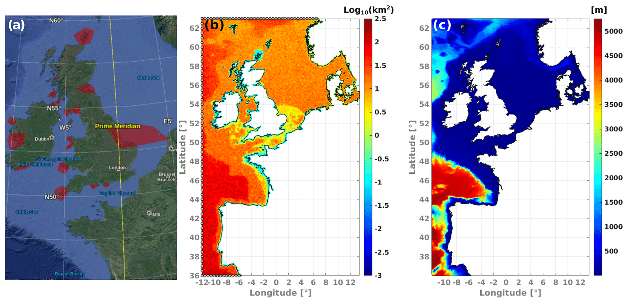
Figure 1 (a) Refinement polygons in red. (b) Final mesh elements size distribution: coastline polygons in black; mesh nodes where boundary conditions are prescribed from the global model in gray. (c) Bathymetry reconstruction with mesh. Color bar in (c) represents depths with respect to mean sea level in meters. Map data in (a) are from © Google Landsat/Copernicus.

An alternative to this careful editing of the mesh is the use of implicit schemes. However, using implicit schemes with CFL values much larger than 1 opens the door to both larger advection errors (stability does not imply accuracy) and larger splitting errors as the time steps for advection can be much smaller than the refraction and source term time step (Roland and Ardhuin, 2014). We have preferred to stick to the explicit Narrow stencil scheme (N scheme) because numerical efficiency is not central in the study, and it simplifies comparisons with global model results that also use explicit schemes. Implicit schemes are probably necessary when resolving regional scales and surf zones in the same mesh when CFL constraints require prohibitively small time steps in explicit schemes.

2.2 Bottom sediment map

The construction of a sediment grain size map was included to properly represent wave energy dissipation due to bottom friction (see Sect. 5.5 for results). In the model, the grain size is characterized by its median diameter D₅₀, defined at each node of the mesh. The D₅₀ values where estimated from the EMODnet harmonized seabed substrate charts. The minimum grain size was set to 0.02 mm, while zones characterized as pebbles or larger elements (boulders) were represented with a D₅₀=150 mm. By default, the minimum grain size was applied to all regions where no substrate was specified. Since most areas with no bottom characterization are in deep waters (e.g., >400 m), this assumption does not have any relevant effect on the wave field evolution. The bottom sediment diameter map is presented in Fig. 2.

2.3 Source terms and numerical choices

In WW3 the wave action equation is solved using a splitting method to treat temporal depth changes, spatial propagation, intra spectral propagation, and source terms (Yanenko, 1971; Tolman and Booij, 1998; The WAVEWATCH III® Development Group, 2019) in different steps. Spectral propagation, which includes refraction, is computed with an explicit third-order scheme that combines the QUICKEST scheme with the ULTIMATE total variance diminishing limiter (Leonard, 1991), while spatial advection is done with the explicit N scheme (Csík et al., 2002; Roland and Ardhuin, 2014). Non-linear evolution and wave to wave interactions are represented with the discrete interaction approximation (DIA, Hasselmann et al., 1985). The utilized wind input and wave dissipation source terms are taken from the ST4 parameterizations described in Ardhuin et al. (2010) with adjustments described in Alday et al. (2021) consistent with the global model used for our boundary conditions. A constant wave energy reflection of 5 % is used at the coastlines, as parameterized by Ardhuin and Roland (2012).

In the present study we only analyze the effects of changes in the ST4 parameterizations. A detailed list of the parameters used for the model implementation is given in Appendix A.

2.4 Boundary conditions and forcing field improvements

The accuracy of modeled wave data directly depends on the quality of the forcing fields and the provided boundary conditions (BCs) for the case of nested models. This becomes particularly relevant in coastal areas for accounting wave–current interactions in macro tidal areas, the assessment of energy resources, port design and operation conditions, or the study of extreme events.

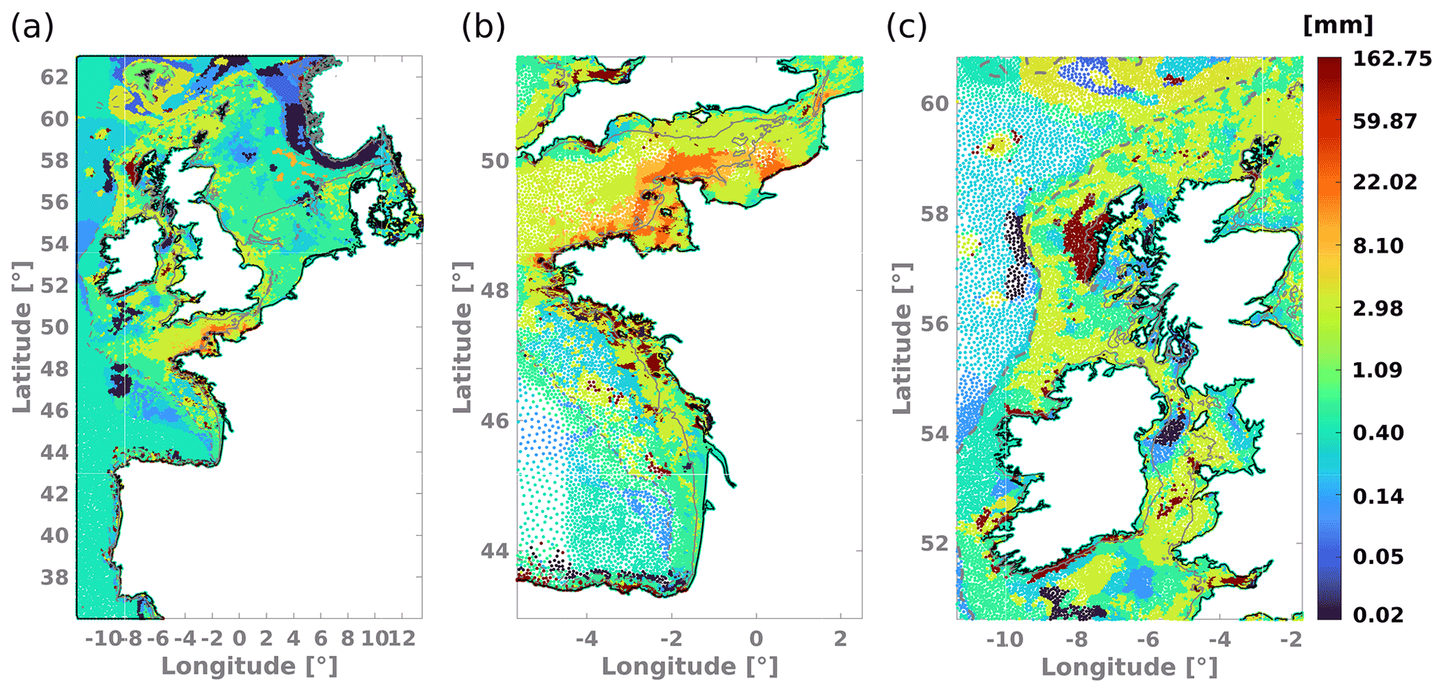
Figure 2 Bottom sediment size map. D₅₀ values assigned to each mesh node for (a) full domain, (b) Bay of Biscay and the English Channel, and (c) United Kingdom. Color bar represents D₅₀ in millimeters. Gray dashed lines represent 20 m depth contours; continuous gray lines represent 50 m depth contours.

Along with the high spatial resolution, an important aspect of the wave hindcast analyzed in this study, is the utilization of improved spectral BC from the wave dataset described in Alday et al. (2021). This wave hindcast was created using wind fields from the fifth-generation ECMWF atmospheric reanalyses of the global climate, ERA5 (Hersbach et al., 2020), and surface current fields taken from the CMEMS Global Ocean Multi Observation Products (MULTIOBS_GLO_PHY_REP_015_004).

The global grid from where boundary conditions are taken has a spatial resolution of 0.5^∘, while the wave spectrum is discretized in 24 directions (15^∘ resolution) and 36 exponentially spaced frequencies from 0.034 to 0.95 Hz with a 1.1 increment factor from one frequency to the next. The proposed spectral discretization, wave growth, and dissipation parameters, along with the use of upgraded forcing fields, showed clear improvements in sea state parameters (at a global scale) when compared to previous hindcasts, like the widely used dataset from Rascle and Ardhuin (2013).

The (directional) spectral BCs taken from the global model are prescribed along the southern, western, and northern open boundaries of the mesh (Fig. 1b). These are interpolated in space and time into each active node along the open boundaries of the nested model.

For the proposed regional model, three main forcing fields were included: wind, tidal levels, and tidal currents. As for the global model, ERA5 surface winds were used for wave generation. Similar to what was done in Boudière et al. (2013), tidal levels and currents time series were reconstructed in WW3 with harmonics taken, in this case, from two different sources. The first one is the output from Ifremer's tidal atlas (Pineau-Guillou, 2013) created with MARS 2D (Lazure and Dumas, 2008), a hydrodynamic model based on the shallow-water equations. A total of five embedded models with three levels of nesting and different spatial resolutions were selected (Fig. 3a). The second tidal data source was used to cover parts of the Atlantic coast of Portugal up to the Gulf of Cádiz which are not included in the tidal atlas. The complement data were taken from the native mesh of the FES2014 model (Carrere et al., 2015) and regridded to 0.004^∘ (Fig. 3b).

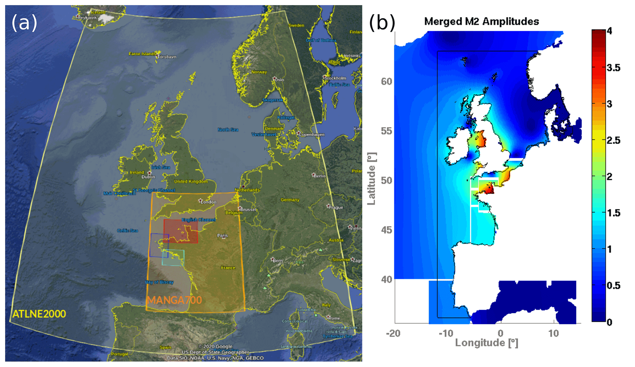
Figure 3 (a) Spatial coverage from selected tidal models. Blue, green, and red rectangles have a 250 m resolution; the orange and yellow area have resolutions of 700 and 2000 m, respectively. (b) Example of merged tidal harmonics from Ifremer's tidal atlas and FES2014. Map data in (a) are from © Google Landsat/Copernicus. Color bar in (b) represents M2 amplitude values in m; black lines show the boundary and coastline polygons.

In all simulations, the boundary conditions are updated every 3 h, winds every 1 h, tidal levels, and velocities fields every 30 min. The output frequency of the nested model is hourly.

2.5 Spectral discretization and time steps

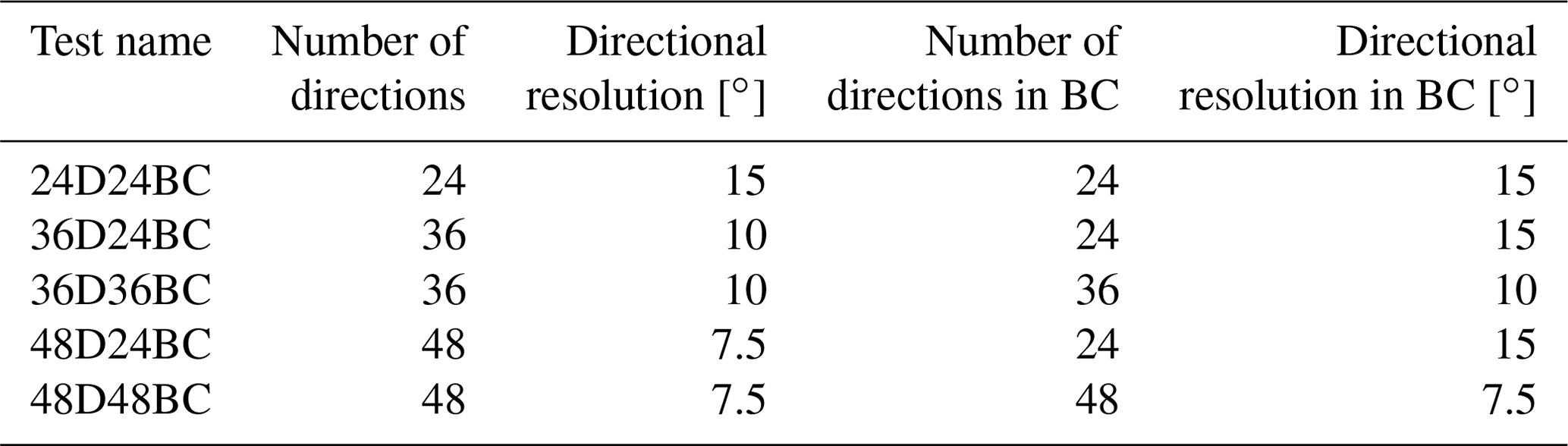
The same extended frequency range used in the global grid was employed in the regional mesh to perform all simulations, matching the discretization at the boundary. The extension to higher frequencies aims to allow for a better representation of the variability of the wave spectrum for very low wind speeds or very short fetches. At the other end, the purpose of adding lower frequencies is to let the spectrum develop longer wave components for severe storm cases (e.g., Hanafin et al., 2012). In terms of directional discretization, we mainly used 36 directions (10^∘ resolution), and tests with 24 and 48 directions were employed to verify the effects of the directional resolution.

The source terms are integrated with an adaptative time step that is automatically adjusted in the range of 5 to 180 s. We defined the maximum model advection time step to be 30 s, taking into account the minimum mesh triangle area and the presence of strong currents. The refraction time step was set to 15 s. Sensitivity tests with smaller values (not shown) had very limited impact on the model results.

3 Wave data sources

3.1 Buoy data

We use six French buoys with spectral data provided by CEREMA (Centre d'études et d'expertise sur les risques, l'environnement, la mobilité et l'aménagement – Centre for Studies on Risks, the Environment, Mobility and Urban Planning) and two Belgian buoys from which spectra were not available, but besides the usual significant wave height, they provide a low-frequency wave height H₁₀ (Fig. 4). The H₁₀ parameter corresponds to a wave height computed for periods from 10 s and longer (≤0.1 Hz). These sites cover a wide range of depths, current intensities, tidal amplitude levels, and proximity to shore, which makes them an appropriate sampling group to evaluate the overall accuracy of the results (Table 1). No assessment of potential instruments' replacements, maintenance periods, or deploy position changes has been taken into account for this study.

Table 1 Spectral buoys ID, location name, position, and estimated deploy depth. Distance to coast estimated with respect to continental coast, except for buoy 62074. Deploy depth obtained from model bathymetry interpolated into the buoys' position. All buoys with spectral data present a frequency range from 0.025 to 0.58 Hz, with a frequency interval of 0.005 Hz.

To match the frequencies discretization of the spectrum and output frequency (hourly) in WW3, spectral data from the in situ measurements have been first interpolated into the same discrete frequencies used in the model and then averaged in time to provide hourly output.

3.2 Satellite altimetry data

Given the advantages of altimeters' spatial coverage, the general performance evaluation of the model results was done by comparing results with the ESA Sea State CCI V2 altimeter dataset. We used the “denoised” (Schlembach et al., 2020; Quilfen and Chapron, 2021) significant wave height (hereinafter wave height) at 1 Hz, to estimate the performance indicators in an along-track statistical analysis of the wave heights and for time-averaged values over the complete modeled domain. The adjusted denoised wave height has an along-track spatial resolution equivalent to approximately 7 km.

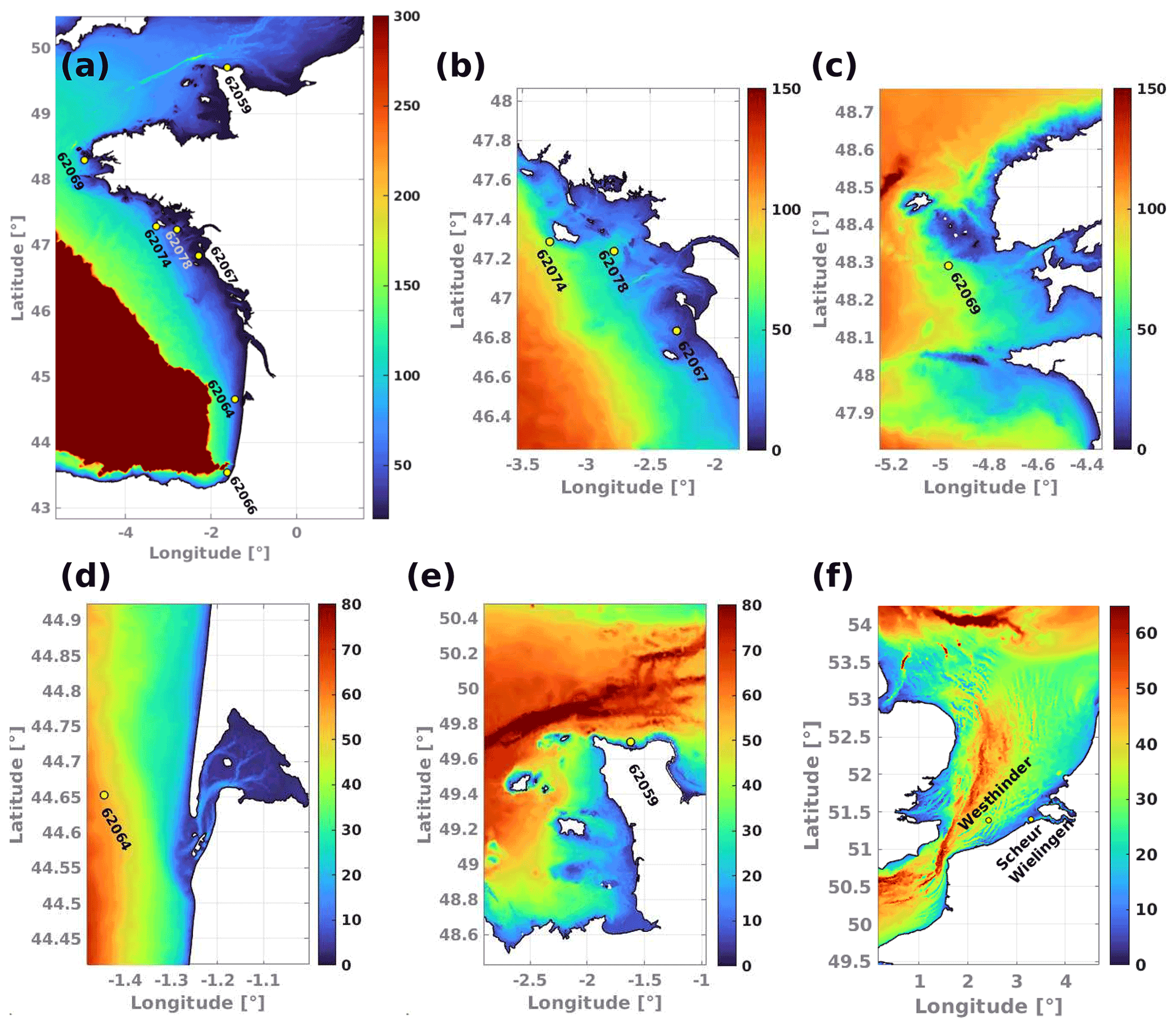
Figure 4 Buoy location and bathymetry features. (a) Buoys along French coast. (b–e) Details of French buoy locations. (f) Detail of Belgian buoy location. Color bar shows depths in meters with respect to mean sea level. Maximum depth on each panel has been selected to enhance bathymetry details.

4 Model performance indicators

We use the following statistical parameters: the root mean squared error (RMSE), normalized root mean squared error (NRMSE), scatter index (SI), mean bias (BIAS), and the normalized mean bias (NMB, hereinafter bias when expressed in percent):

$$\begin{array}{}\text{(1)}& {\displaystyle }\text{RMSE}\left(X\right){\displaystyle }=\sqrt{{\displaystyle \frac{\sum (X_{\text{mod}}-X_{\text{obs}}{)}^{\mathrm{2}}}{N}}},\end{array}$$

$$\begin{array}{}\text{(2)}& {\displaystyle }\text{NRMSE}\left(X\right)& {\displaystyle }=\sqrt{{\displaystyle \frac{\sum (X_{\text{mod}}-X_{\text{obs}}{)}^{\mathrm{2}}}{\sum X_{\text{obs}}^{\mathrm{2}}}}},\text{(3)}& {\displaystyle }\text{SI}\left(X\right)& {\displaystyle }=\sqrt{{\displaystyle \frac{\sum {\left[(X_{\text{mod}}-\stackrel{\mathrm{‾}}{X_{\text{mod}}})-(X_{\text{obs}}-\stackrel{\mathrm{‾}}{X_{\text{obs}}})\right]}^{\mathrm{2}}}{\sum X_{\text{obs}}^{\mathrm{2}}}}},\text{(4)}& {\displaystyle }\text{BIAS}\left(X\right)& {\displaystyle }={\displaystyle \frac{\mathrm{1}}{N}}\sum (X_{\text{mod}}-X_{\text{obs}}),\text{(5)}& {\displaystyle }\text{NMB}\left(X\right)& {\displaystyle }={\displaystyle \frac{\sum (X_{\text{mod}}-X_{\text{obs}})}{\sum X_{\text{obs}}}},\end{array}$$

where X_obs is the observed quantities from in situ or satellite measurements, X_mod is the modeled quantities (spectral values or integrated wave parameters), and N is the total number of analyzed data.

We use the term normalized mean differences (NMDs) when using Eq. (5) between different model configurations.

5 Sensitivity analyses results and discussion

5.1 Influence of spatial resolution

We first consider significant wave heights (hereinafter H_s or “wave height”). A comparison between February 2011 mean H_s fields from the global model described in Sect. 2.4 and our implemented regional model is presented in Fig. 5. To evaluate the differences between models, the output from the 0.5^∘ global grid was linearly interpolated onto the regional mesh nodes before computing the mean wave height and the mean difference for the selected time window.

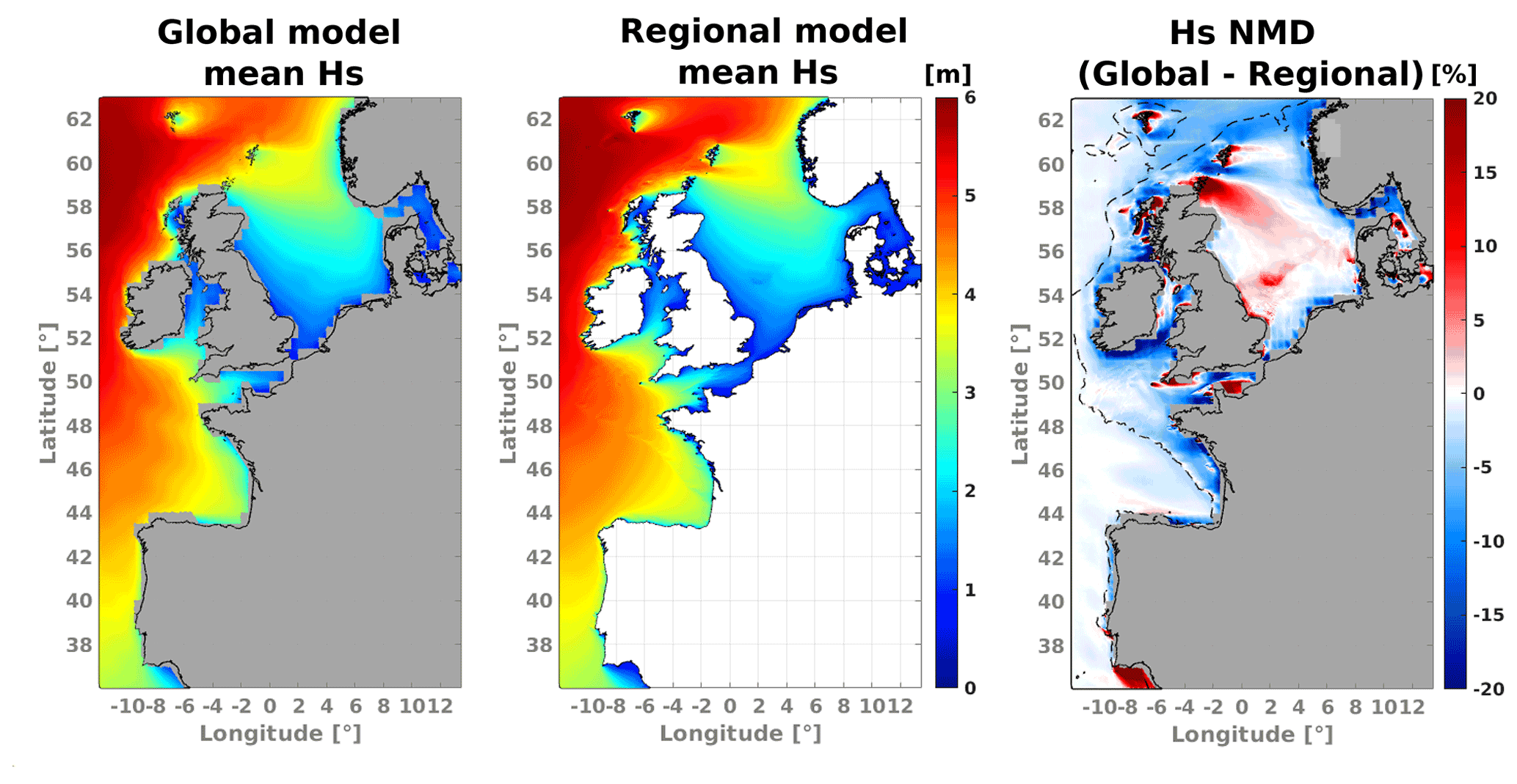
Figure 5 Mean wave height fields from global and regional models and wave height normalized mean differences (NMDs: global−regional). Dashed black lines represent the 400 m depth contours. Areas where no wave data are available from the global grid are highlighted with a gray background in left and right panels. Results for February 2011.

The most important differences are found on the shelf, where complex coastline geometry and bathymetry requires higher detail to better represent land shadows and wave refraction (NMD in Fig. 5). The largest positive differences (>20 %) are commonly found in the regions sheltered from North Atlantic swells. In the global model, islands and headlands smaller than the grid size are parameterized as obstructions of the wave energy flux (Chawla and Tolman, 2008). Another direct effect of using increased spatial resolution can be seen between the Orkney and the Shetland islands. The regional model shows averaged wave height values of almost 5 m in this area for the analyzed month. On the other hand, the combined effects of the sub-grid obstruction approach and coarse resolution of the global grid lead to high underestimation of about −20 % with respect to our mesh results.

5.2 Adjustments in wind-wave generation and swell dissipation

Alday et al. (2021) adjusted the parameterizations of wind-wave generation and swell dissipation proposed by Ardhuin et al. (2010) and Leckler et al. (2013), these adjustments were designed to better represent the wave heights measured by altimeters at global scales. Here we further consider the impact of these modifications on waves in our coastal domain, using five different simulations with parameter changes listed in Table 2. These changes include an empirical enhancement of the wind speeds above a threshold U_c by the amount x_c(U₁₀−U_c) and a modification of the swell dissipation with a change in the threshold Reynolds number Re_c that defines the transition from the weak (laminar) to strong (turbulent) swell dissipation and the swell dissipation coefficient s₇.

Table 2 Tests for wind correction and swell dissipation parameters. All parameters not specified here correspond to the T475 parameter adjustment detailed by Alday et al. (2021). Variables Re_c, U_c, and x_c correspond to namelist parameters SWELLF7, SWELLF4, WCOR1, and WCOR2 in the WW3 input files (see Appendix A for the full set of parameters). The directional discretization has 24 directions in all of these tests.

We analyzed model results for 2 months when extreme sea states have been recorded: February 2011 and January 2014. In February 2011, the extra tropical storm Quirin generated extreme sea states with peak periods exceeding 20 s over the western coasts of Europe. In January 2014, storm Hercules was one of the many storms from a particularly severe winter. This event caused vast coastal damage in the United Kingdom (Masselink et al., 2016) and from the western coast of France to Portugal (Masselink et al., 2015). Wave height values exceeded 10 m and peak periods exceeded 20 s (Ponce De León and Soares, 2015; Castelle et al., 2015). Given the characteristics of the selected cases, it is considered that they are suitable to study wave energy fluctuations down to frequencies lower than 0.06 Hz. Although analyses were carried out for February 2011 and January 2014, in this section we only present the results for the later period.

Despite the similarities between time series of the wave parameters such as H_s and T_m02 from one test to another, they differ noticeably for extreme values. Yet, the model runs have systematic differences as a function of wave heights or wave periods, with 5 % to 10 % deviations for the larger periods and heights that correspond to the most severe storms and associated swells (Fig. 6). In these events, and consistent with the global-scale results, the wind enhancement is most effective at correcting the low bias in extreme wave heights and mean periods that is typical of the previous hindcasts. Adjustments to the swell dissipation have a negligible impact when acting only 1000 km or less of propagation within our coastal domain. As shown in Fig. 7, the wind enhancement allows the generation of lower-frequency waves. This improves the model accuracy at exposed buoys 62066, 62074, and 62069 and produces realistic energy levels for frequencies below 0.05 Hz during the extreme events of January 2014. Unfortunately, the correction also produces too much low-frequency energy at the shallower buoy 62078. We suspect that dissipative processes in shallow water may be underestimated for these very large periods (Fig. 7e and f).

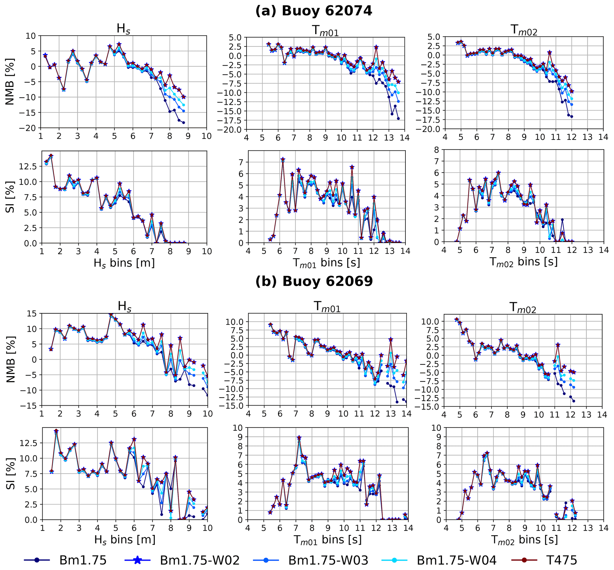
Figure 6 Bias (NMB) and scatter index (SI) for tests leading to T475 (Table 2). Results for January 2014. In (a) and (b) modeled results are compared with buoys 62074 and 62069, respectively. H_s bin size is 0.25 m; periods bin size is 0.2 s. T_m01 and T_m02 are computed integrating the spectra in the frequency range 0.0339–0.537 Hz.

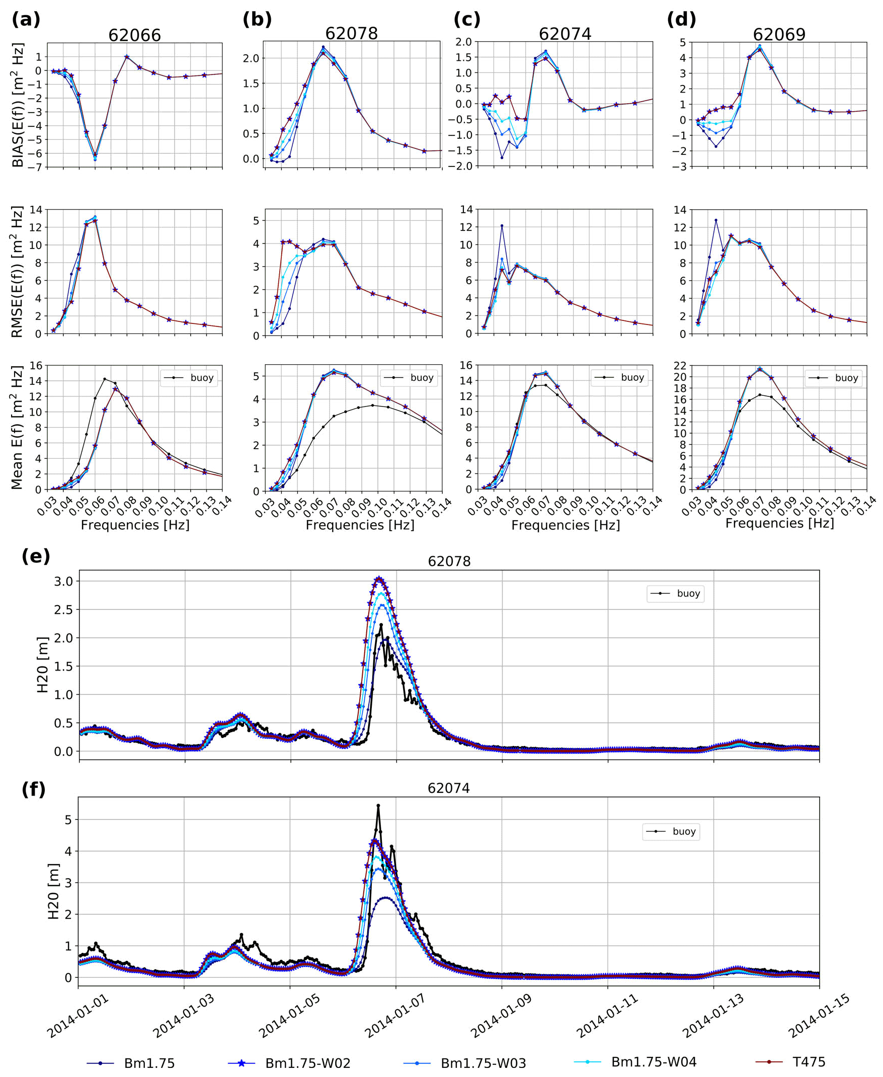
Figure 7 Performance parameters for energy levels at each discrete frequency of the spectrum, for tests leading to T475 (Table 2). Results for January 2014 at buoys 62066, 62078, 62074, and 62069. In panels (a–d) 1-month modeled results compared with buoy data. Time series of modeled and measured H₂₀ for buoys 62078 in (e) and 62074 in (f).

5.3 Wave–current interactions

At a global scale, the use of ocean surface currents can improve the accuracy of the simulated sea states (Echevarria et al., 2021; Alday et al., 2021), although a full effect generally requires relatively high spatial resolution that is generally not achievable by observations, and thus models are usually not constrained at the necessary scale (Marechal and Ardhuin, 2020). This is the main reason why geostrophic currents were not considered in the high-resolution regional model.

Adding surface currents in the simulations can have effects on wave generation due to changes in the relative wind; it can modify the advection of waves or induce refraction in regions with large current gradients. Given the diverse tidal amplitudes within the modeled domain, it is expected to have different effect levels over the sea states in different areas. We thus attempt to characterize the changes in the wave field when tidal currents are taken into account in the simulations. To do so, we look at differences in a set of wave parameters, namely H_s, directional spreading SPR, the peak direction D_p, and peak period T_p. We first checked global-scale current effects via the boundary conditions and then focused on tidal current effects within our coastal domain.

To evaluate the effects of global currents on the boundary condition, we analyzed a specific output time with a large Atlantic swell and differences between 1-month simulations. The most noticeable changes caused by global currents are obtained for H_s, D_p, and directional spreading (Fig. 8 middle panels), with typical differences of the order of 5 %. These differences vanish when averaged over 1 month (Fig. 8 right panels).

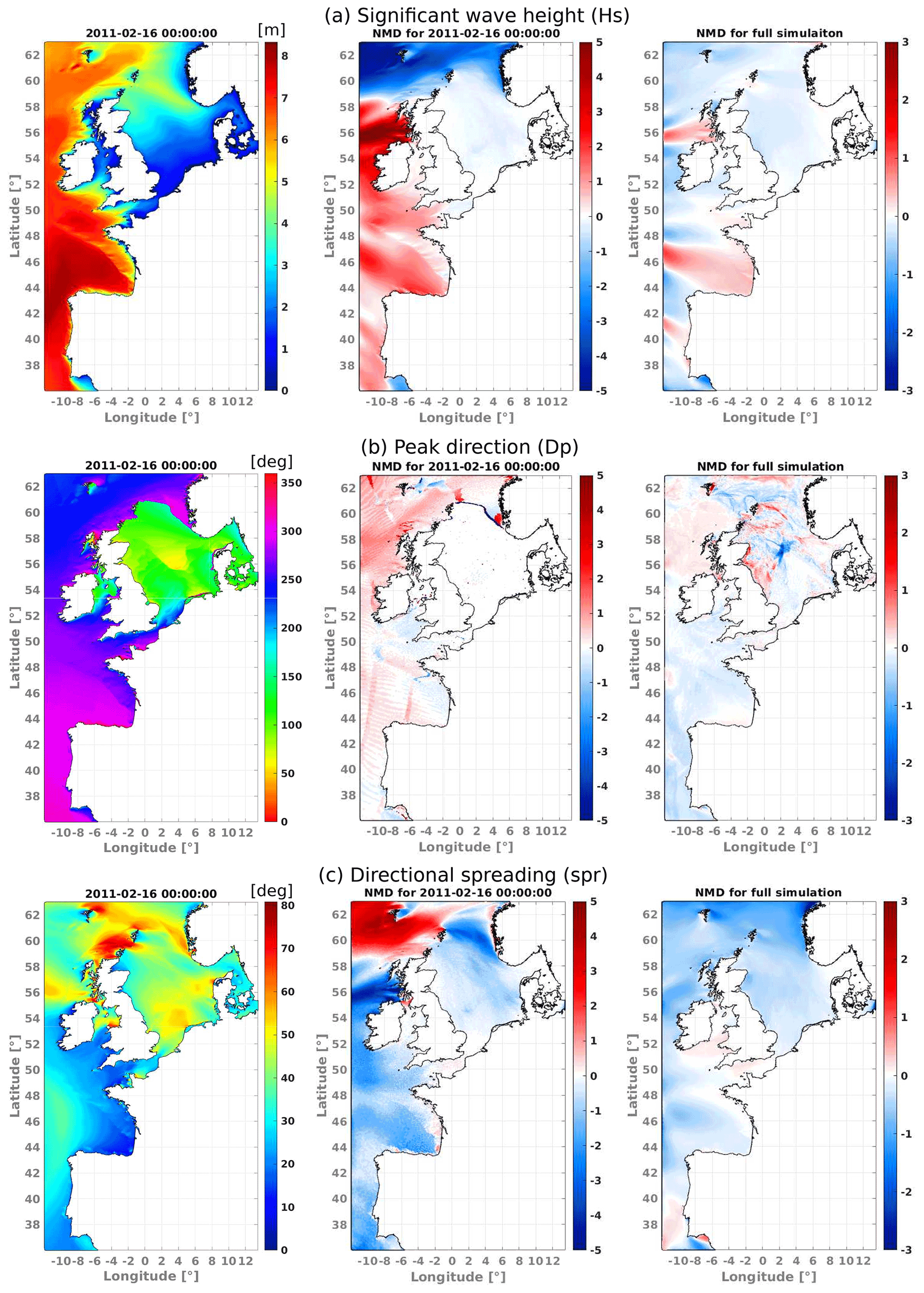
Figure 8 Global current effects over (a) H_s, (b) D_p, and (c) directional spreading. In the left panels, model output for a test using BC generated with global currents from 16 February 2011, 00:00:00 UTC. Mean difference results in the middle and right columns are for a test with BC obtained without global surface currents with respect to a test with BC from a global grid forced with global currents. Color bars in the middle and left panels give the normalized mean difference value in percent. Full simulation duration of tests is 1 month.

The effects of tidal currents within the model domain are generally more important, with some strong local effects caused by the high spatial currents' variability. In contrast to the influence of global currents in the BC, there is a clear increase in the wave fields' differences at each temporal output that can be larger than ±10 %, a feature mainly seen along the English Channel and the Irish Sea (Fig. 9, left panels). Over the entire month, tidal currents induce mean wave height differences of the order of 5 % (Fig. 9, right panels).

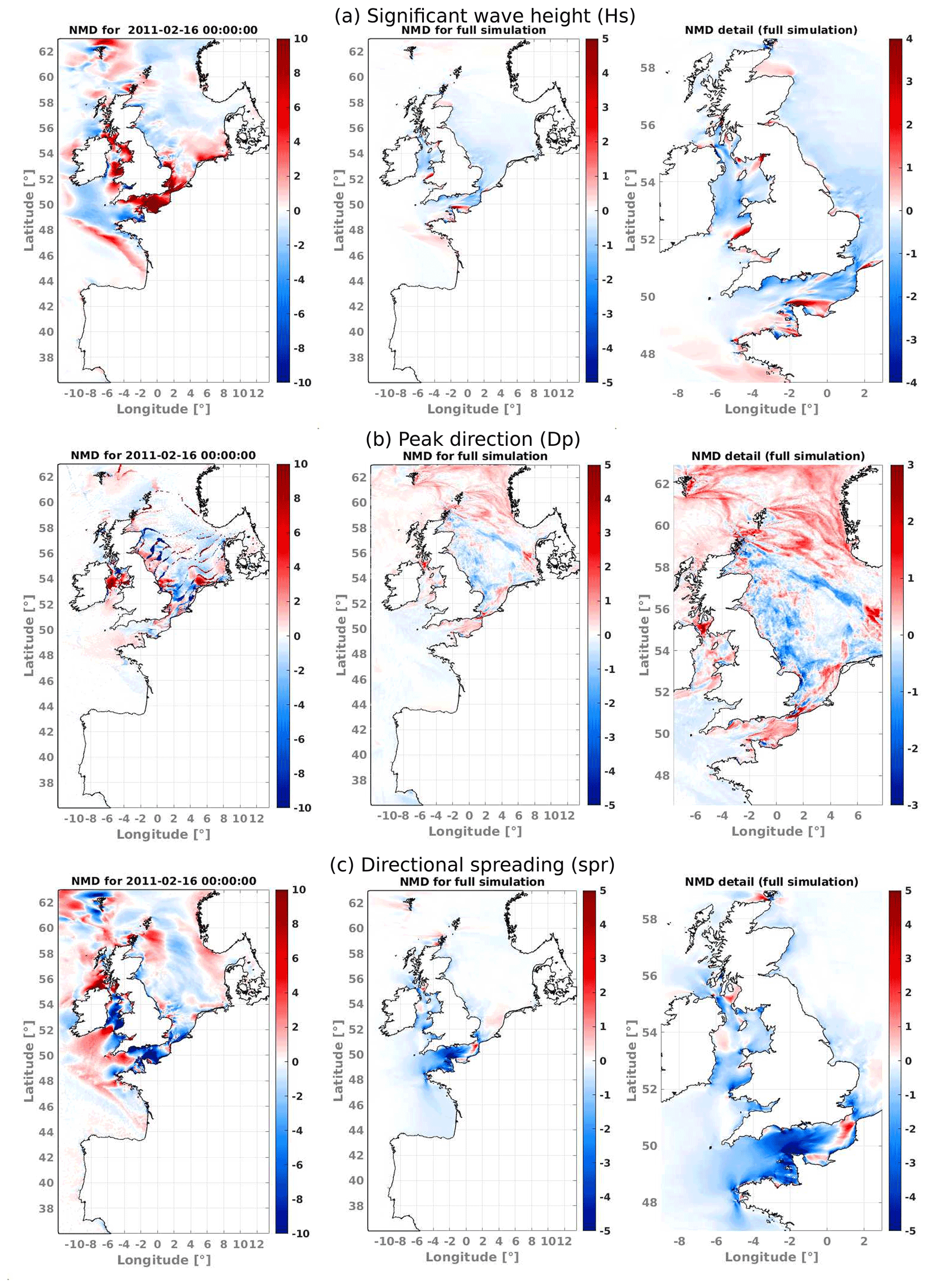
Figure 9 Tidal current effects over (a) H_s, (b) D_p, and (c) directional spreading. Differences are obtained with respect to a test using tidal currents. In the left panels, the difference with respect to model output from 16 February 2011, 00:00:00 UTC presented in the left panels of Fig. 8. Color bars in the middle and left panels give the normalized mean difference value in percent. Full simulation duration of tests is 1 month.

The use of tidal currents also proved to have a large impact over the peak period (T_p): up to 15 % differences in Normandy and Liverpool Bay, for example, and 8 % mean differences over 1 month (not shown).

There is a noticeable feature of the wave field along the shelf break, starting at the Bay of Biscay and extending northwards up to 49^∘ N, which can be seen more clearly through the D_p and H_s fields from Fig. 8a and b (left panel) and particularly by analyzing the effects of tidal currents over the wave heights in Fig. 9a (left panel). The intensities of current used in our model present maximum values of about 0.5 m s⁻¹ along the aforementioned area, which is consistent with previously recorded in situ measurements and the expected sharp variation in currents across the shelf break (i.e., Le Cann, 1990). It is thought that the distinct gradients visible in some of the wave parameters are function of the tides' phase and the mean wave direction. Attempts to identify the presence of this signature with altimeter data are an ongoing subject of study.

Results were further compared against in situ data from January 2014 at buoy 62059 (Fig. 10). Including tidal currents helps to reduce the high energy bias at low frequencies, probably due to an overall reduction in the effective wind input for locally generated waves during the tidal cycle (Fig. 10a). In Fig. 10c is possible to observe the modulation of H_s and T_m01 caused by the changes in current intensities and direction (blue line in figure), which in the end helps to reduce the bias of these quantities compared to the measurements (Fig. 10b). Notice that there is a constant shift in the occurrence of peaks and troughs of H_s and T_m01 in Fig. 10c. This is thought to be mostly attributed to a slight phase shift in the tidal forcing field, which introduces a slight increase in the root mean square error when tidal currents are included in the simulations (not shown).

Figure 10 Evaluation of tidal current effects on wave energy distribution (a): H_s and T_m01 at buoy 62059 (Cherbourg Exterieur). Wave parameters' NMB and time series in (b) and (c), respectively. Results for January 2014. H_s bin size is 0.25 m; T_m01 bin size is 0.2 s.

5.4 Effects of spectral directional resolution

The selection of the spectral discretization plays an important role in the characteristics of the modeled sea states (Tolman, 1995a; Roland and Ardhuin, 2014). Normally, in coastal applications like assessments of wave energy or simulation of storm surges, higher time and spatial variability details are desired and, hence, higher spatial and spectral resolution is required (e.g.,   Bertin et al., 2015; Accensi et al., 2021; Wu et al., 2020). Nevertheless, the quality of the results may be affected by the characteristics of the BC used.

We analyzed the changes in the energy distribution of the directional spectrum and the wave field evolution due to different directional-resolution values in our mesh and in the BC. The different BC tests are aimed to identify potential effects when coarser resolution is used at a global scale, and then interpolation is applied to match the resolution of the nested mesh (this is done in WW3). Then, to eliminate the potential influence of energy interpolation at the boundary, we verified the effects on wave propagation within the mesh domain keeping consistent resolutions at the BC and the nested model. For example, the difference between 48D24BC and 48D48BC is that the boundary conditions (BCs) were created in a global model with different spectral resolution. Test 48D24BC employs boundary conditions from a global model with 24 discrete spectral directions equivalent to 15^∘, which are then interpolated (in WW3) into 48 directions to match the mesh resolution (48D). On the other hand, in test 48D48BC we used boundary conditions from a global model which has a spectral directional resolution of 7.5^∘ (48 directions), the same used in the high-resolution mesh; hence, no directional interpolation of the spectrum is required. Tests' specifications are defined in Table 3.

Table 3 Tests for spectral directional-resolution effects. All parameters not specified here correspond to test T475. When the directional resolution of the boundary conditions (BCs) is lower than in the mesh, interpolation is applied at the boundary to match the resolution of the nested model.

Variations in the energy distribution due to lower resolution in the BC are presented in Fig. 11, comparing BC with 24 spectral directions with respect to 36. A set of four locations were selected: at the boundary (named node W12N56) and along the French coast nodes 62074 (Belle Ile), 62069 (Pierres Noires), and 62059 (Cherbourg). Bathymetry details of these locations are presented in Fig. 4. Here we present results for January 2014, but the analysis was also conducted with simulations for February 2011.

At the boundary, most of the difference in energy traveling outside the domain is related to very low levels of spectral energy (angles >270 and <360^∘, Fig. 11a right panels). This has negligible effects on the already analyzed wave parameters (e.g.,  H_s, D_m, SPR). For waves traveling into the domain, only large differences ($\text{NMD}>\pm \mathrm{10}$ %) are observed at lower frequencies (<0.1 Hz) between directions 20 and 150^∘ (Fig. 11a right panel), which corresponds to the area with higher mean energy at this location for January 2014 (defined by the contours in the “mean energy” panel of Fig. 11a). We found that this effect is still present in nearshore areas exposed to the incoming swells from the North Atlantic (nodes 62074 and 62069), although with an overall narrower directional range attributed mostly to the bathymetry-induced refraction that tends to “align” the arriving waves (Fig. 11b and c).

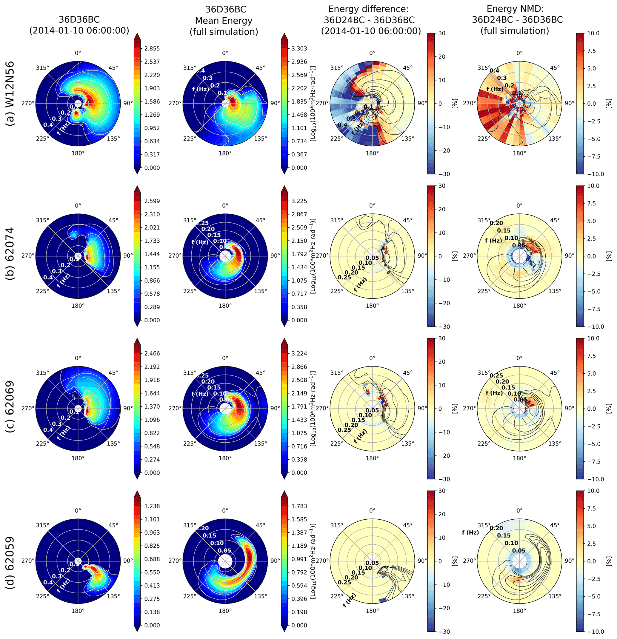
Figure 11 Effects of boundary conditions with lower directional resolution at different output locations. (a) Boundary node W12N56 (long: 12^∘; lat: 56^∘) (b) 62074 (Belle Ile), (c) 62069 (Pierres Noires), and (d) 62059 (Cherbourg). Absolute and normalized differences (36D24BC−36D36BC) computed for January 2014. White contours marking energy levels in the left panels are overlaid in black in the difference plots. The direction convention defines the travel direction of the energy.

No significant changes in energy distribution were found at node 62059, for each output time and for the full simulation (Fig. 11d). This is expected since at Cherbourg the sea state characteristics are mostly driven by the local winds.

To further assess potential changes introduced in wave parameters, we analyzed the differences in fields of H_s, T_p, SPR, D_p, and the mean direction D_m (not shown; Fig. 12). Using a coarser directional resolution in the BC has minor effects over wave parameters integrated along the complete frequency range (e.g., D_m or H_s; Fig. 12b, top panels). Differences in the results are exacerbated when BCs with 24 directions are interpolated into 48 (right panels in Fig. 12a and b) but in general mean and random differences between tests remained below ±2.5 %, with the exception of T_p, which presented the largest normalized root mean squared differences (NRMSDs).

Figure 12 (a) Normalized mean differences (NMDs) and (b) normalized root mean squared differences (NRMSDs) between tests 36D24BC−36D36BC and 48D24BC−48D48BC. Analyzed period: February 2011. Color bars represent changes in quantities between tests in percent.

Even though the magnitude of these quantities remains fairly consistent, interpolating BC with a coarser directional resolution affects the characteristics of the wave fields propagating into the domain. This is attributed to slight changes in the wave celerity ($C=gT/\mathrm{2}\mathit{\pi }$ in deep waters) due to frequency shifts in the neighborhood of the energy peak (Fig. 11a–c, “energy difference panels”).

The analysis of the directional resolution of the mesh is mainly focused on the garden sprinkler effect (GSE) on wave propagation. This phenomenon is observed as a separation or disintegration of continuous swell fields propagated with a discretized spectral wave model (Booij and Holthuijsen, 1987; Tolman, 2002). The generation of the GSE is linked to the spectral resolution and the advection scheme. Currently there are no GSE alleviation methods available for unstructured grids in WW3.

A good example was found in 1 February 2011, where a strong swell from the North Atlantic arrived at the northern coast of Scotland. In Fig. 13a we present an instant (13:00:00 UTC) of the event using three different discretizations from tests 24D24BC, 36D36BC, and 48D48BC (Table 3). The GSE can be observed to the east of the Orkney and Shetland islands towards the Norwegian Sea (between latitudes 58 and 61^∘) when 24 directions are employed (Fig. 13a, left panel).

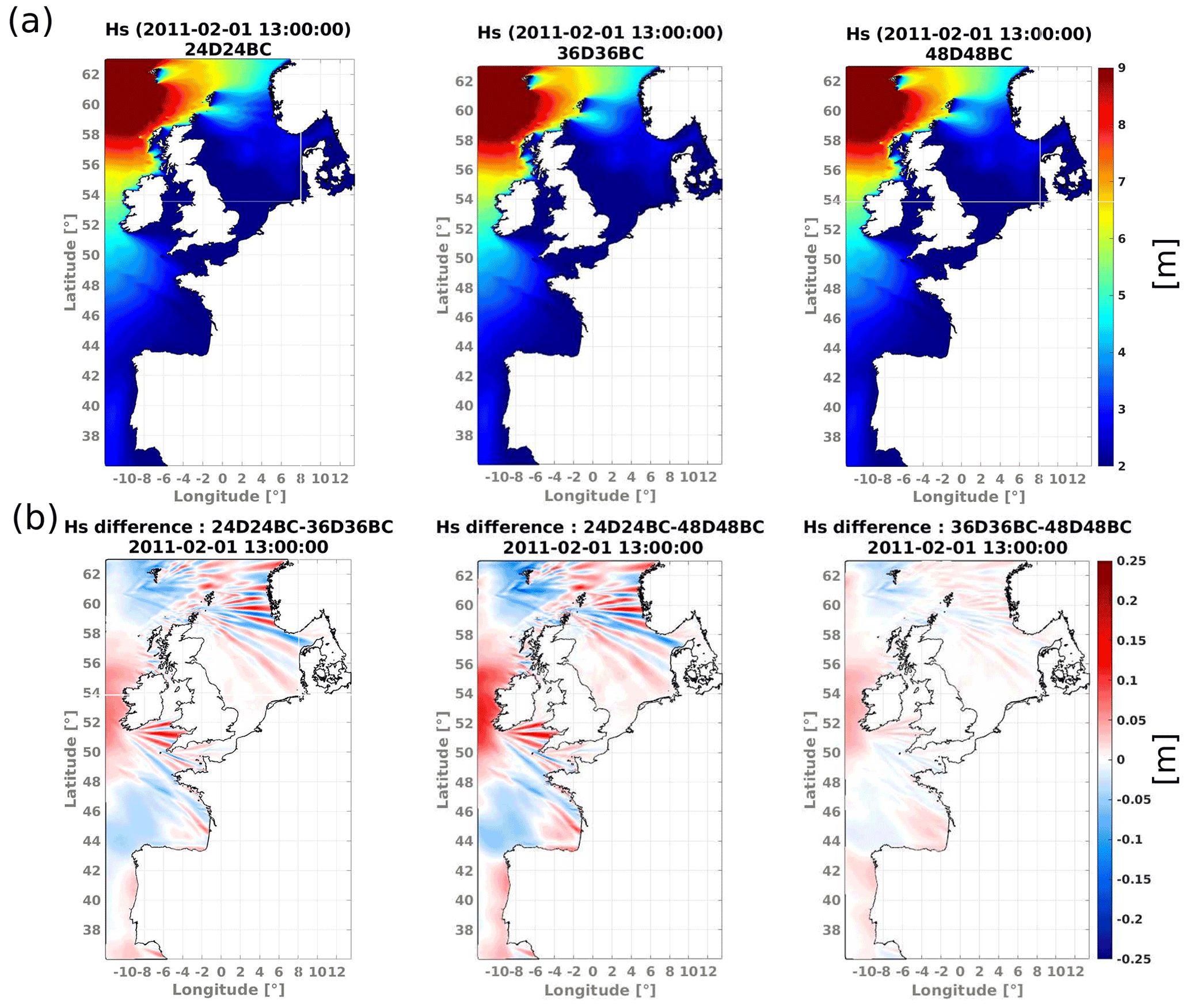
Figure 13 (a) Wave height field from 1 February 2011, 13:00:00 UTC, for different directional-resolution tests specified in Table 3. (b) Differences in wave height fields presented in (a). Offshore swell conditions (to the west of the Orkney and Shetland islands): $T_{\mathrm{p}}=\sim \mathrm{14}$ s; $D_{\mathrm{m}}=\sim \mathrm{260}$^∘.

The impact of the GSE was assessed by comparing the results against the output from a model with a higher directional resolution. Via a straightforward difference between tests, it is possible to visualize changes in the H_s field caused by the spurious wave propagation pattern (Fig. 13b). Comparing test 24D24BC with 36D36BC, and for this particular scenario, differences in wave height can reach ±0.2 m (roughly ±5 %) as the swell approaches Norway, between longitudes 2 to 4^∘ E (Fig. 13b, left panel). These values are only slightly higher when comparing tests with 24 to 48 directions (Fig. 13b, middle panel). Between 36D36BC and 48D8BC, only minor H_s changes are generated (<0.05 m; Fig. 13b, right panel).

The mild repercussion of the GSE over the wave height field in the present results should not be generalized, since this phenomenon could be intensified depending on the incoming swell conditions. Our findings suggest that using a directional resolution of 10^∘ is enough to mitigate the effects of the GSE. It is relevant to point out that, for example, the required computation time in 36D36BC is 40 % higher than in 24D24BC, a considerably elevated cost for potential operational (forecasting) applications.

5.5 Bottom friction effects

Over the continental shelf, in intermediate to shallow waters, the evolution of the wave fields becomes influenced by the bottom characteristics. In the absence of strong wind seas and outside the surf zone, the dissipation of energy is mainly induced by bottom roughness effects. We thus try to quantify the effects of including the bottom friction sink term in the wave action equation.

To provide a general view, we compared model output from 1-year tests with the 1 Hz altimeter data from the ESA Sea State CCI V2 dataset. For this particular analysis 1-year simulations were required in order to have at least a minimum of five satellite measurements to compare with the regridded WW3 wave height fields at 0.1^∘. Only altimeter measurements at least 10 km away from the coastline were considered to avoid potential data with a high noise-to-signal ratio.

Bottom friction effects were included through the SHOWEX parameterization proposed in Ardhuin et al. (2003). This expression was initially developed for sandy bottoms based on the eddy viscosity model of Grant and Madsen (1979) and includes a decomposed roughness parameterization for ripple formation and sheet flow. In WW3 it has been implemented, including a sub-grid parameterization for water depth variability following Tolman (1995b). The bottom friction source term can be written as follows:

$$\begin{array}{}\text{(6)}& S_{\text{bot}}=f_{\mathrm{e}}{u}_{\text{b,rms}}{\displaystyle \frac{{\mathit{\sigma }}^{\mathrm{2}}}{\mathrm{2}g\times {\sinh }^{\mathrm{2}}\left(kd\right)}}N(k,\mathit{\theta }),\end{array}$$

with

$$\begin{array}{}\text{(7)}& f_{\mathrm{e}}={\displaystyle \frac{{\mathit{\kappa }}^{\mathrm{2}}}{\mathrm{2}\left({\text{Ker}}^{\mathrm{2}}\left(\mathrm{2}\sqrt{\frac{z_{\mathrm{o}}}{l}}\right)+{\text{Kei}}^{\mathrm{2}}\left(\mathrm{2}\sqrt{\frac{z_{\mathrm{o}}}{l}}\right)\right)}},\end{array}$$

and

$$\begin{array}{}\text{(8)}& {\displaystyle \frac{z_{\mathrm{o}}}{l}}=\sqrt{{\displaystyle \frac{\mathrm{2}}{f_{\mathrm{e}}}}}{\displaystyle \frac{k_{\mathrm{N}}}{\mathrm{30}\mathit{\kappa }{a}_{\text{b,rms}}}}.\end{array}$$

When the Shields number ψ is ≥A₃ψ_c, the Nikuradse roughness k_N is taken as the sum of the ripple roughness k_r and a sheet flow roughness k_s:

$$\begin{array}{}\text{(9)}& {\displaystyle }{k}_{\mathrm{r}}& {\displaystyle }=a_{\text{b,rms}}\times A_{\mathrm{1}}{\left({\displaystyle \frac{\mathit{\psi }}{{\mathit{\psi }}_{\mathrm{c}}}}\right)}^{A_{\mathrm{2}}},\text{(10)}& {\displaystyle }{k}_{\mathrm{s}}& {\displaystyle }=\mathrm{0.57}{\displaystyle \frac{u_{\text{b,rms}}^{\mathrm{2.8}}{a}_{\text{b,rms}}^{-\mathrm{0.4}}}{\left[g\right(s-\mathrm{1}\left){]}^{\mathrm{1.4}}\right(\mathrm{2}\mathit{\pi }{)}^{\mathrm{2}}}},\end{array}$$

where

$$\begin{array}{}\text{(11)}& {\displaystyle }\mathit{\psi }& {\displaystyle }={\displaystyle \frac{f_{\mathrm{w}}{u}_{\text{b,rms}}^{\mathrm{2}}}{g(s-\mathrm{1})D_{\mathrm{50}}}},\text{(12)}& {\displaystyle }{\mathit{\psi }}_{\mathrm{c}}& {\displaystyle }={\displaystyle \frac{\mathrm{0.3}}{\mathrm{1}+\mathrm{1.2}{D}_{*}}}+\mathrm{0.55}[\mathrm{1}-\exp (-\mathrm{0.02}{D}_{*}\left)\right],\end{array}$$

with

$$\begin{array}{}\text{(13)}& D_{*}=D_{\mathrm{50}}{\left[{\displaystyle \frac{g(s-\mathrm{1})}{{\mathit{\nu }}^{\mathrm{2}}}}\right]}^{\mathrm{1}/\mathrm{3}}.\end{array}$$

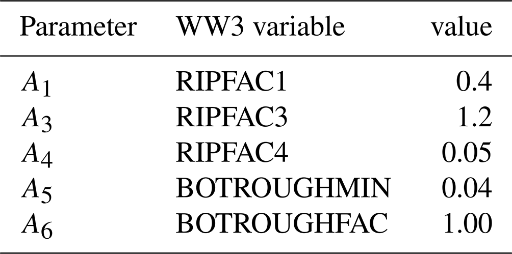
In Table 4 we present a set of empirical parameters originally taken from Ardhuin et al. (2003), where we have particularly modified A₅ to 0.04. D₅₀ is the median sediment size in meters defined at each node of the unstructured grid (see Fig. 2). A full description of the terms in Eqs. (6) to (13) can be found in Ardhuin et al. (2003) and in the WW3 user manual (The WAVEWATCH III® Development Group, 2019).

Table 4 List of empirical parameters used in SHOWEX bottom friction parameterization. The WW3 variables' names correspond to the keyword used in the model's BT4 namelist.

To assess the effects of the bottom friction parameterization, we first compared 1-year simulations with and without dissipation to verify changes in the wave field. In Fig. 14a we present the wave height mean bias obtained by comparing it with Saral (year 2014) for the full domain. A clear reduction in the wave height bias is detected in the south of the North Sea. In this area, we found that wave height mean differences between results with and without bottom friction can be 0.3 m and higher. Analysis with other altimeters (e.g., Jason-2 and Envisat) for the year 2011 show consistent results.

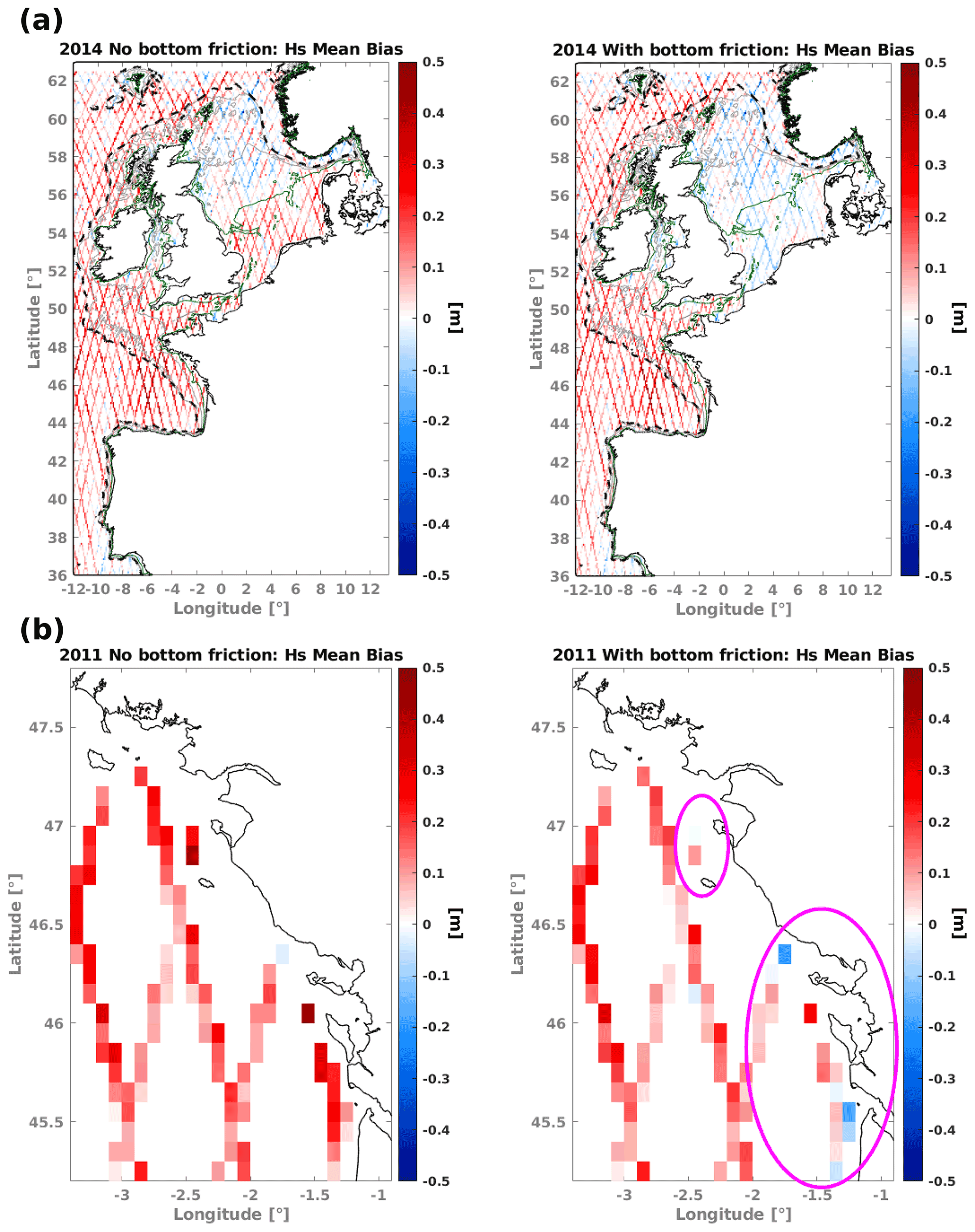
Figure 14 Wave height bias (WW3 – altimeter) computed with (a) Saral for the year 2014 and (b) Envisat for the year 2011. Dashed black lines show the 200 m depth contour, green lines the 50 m depth contours, and gray lines depth contours from 100 to 150 m depth. Magenta ovals in (b) highlight areas with the largest bias reduction.

In general, with altimeter data most relevant changes in wave heights, when bottom friction is included, are detected for depths smaller than 50 m. We found a couple of Envisat tracks passing almost parallel off the coast of La Rochelle and close to Ile de Yeu (Fig. 14b). In both locations the use of the bottom friction parameterization, with the defined D₅₀, helps to reduce the mean bias in wave heights. These results are consistent with the findings of Roland and Ardhuin (2014) for this area based on buoy data.

We picked three locations to compare our results with in situ measurements: buoy 62078 on the Atlantic French coast and buoys Westhinder and Scheur Wielingen deployed in shallower depths along the coast of Belgium (Fig. 4).

For buoy 62068 we first compared the full time series of in situ wave height against simulations with and without bottom friction effects. Reductions in the wave height bias and NRMSE of, respectively, 4.5 % and 5.0 % are obtained when bottom friction and the sediment size map are included (Fig. 15a and c). Nevertheless, the most significant changes in the modeled wave height appear at wave heights roughly larger than 3 m. We then selected an ad hoc wave height threshold of 3.5 m to define “extreme” sea states and analyze the effects of the parameterization over the events in which dissipation due to wave–bottom interactions is dominant. For these events, a wave height bias and RMSE reduction of about 0.3 m, with a decrease of about 8 % and 5.3 % in the bias and scatter are obtained when the SHOWEX dissipation term is used (Fig. 15b). Moreover, we found good agreement between the occurrences of the Shields number ψ exceeding its critical value ψ_c (Fig. 15d) and the occurrences of extreme sea states with H_s>3.5 m (Fig. 15c) especially between January and March 2014. In the model, the evolution timescale due to bottom friction is inversely proportional to f_eu_b,rms, which gives a measure of the strength of bottom friction, sharply increasing every time the critical Shields number is exceeded. In this case, the definition of extreme events helps to identify when the effects of bottom friction become relevant, since larger H_s is normally related to longer wavelengths; thus wave–bottom interactions start at deeper depths.

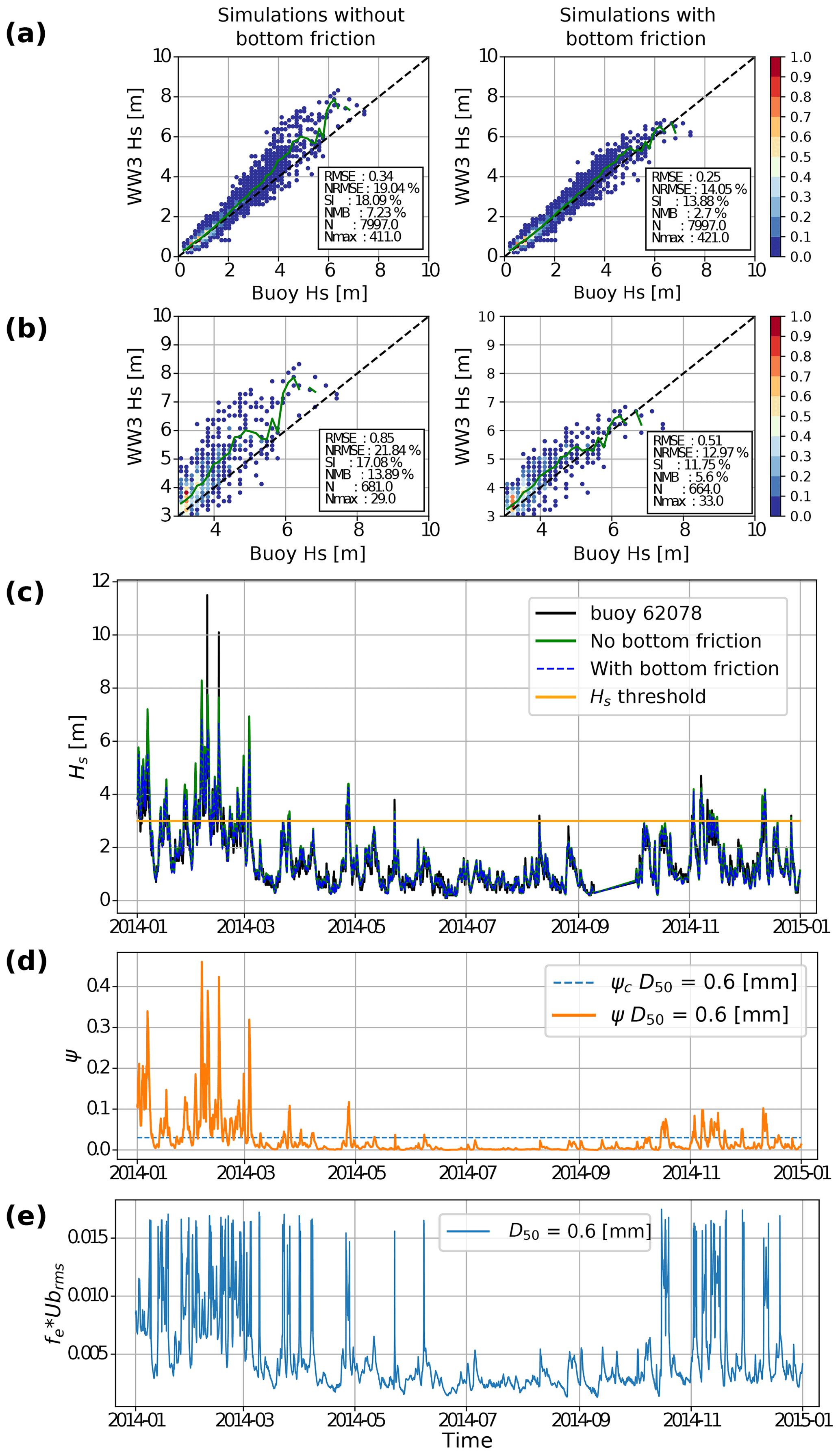
Figure 15 Bottom friction effects at buoy 62078 (year 2014). Performance analysis using (a) complete time series and (b) extreme events (H_s>3.5 m). (c) H_s time series for cases with and without SHOWEX parameterization. Time series of (d) Shields number ψ and (e) dissipation term f_eu_b,rms. In (a) and (b) green line shows the modeled averaged values at each 0.15 m wave height bin. Color bars represent the wave height frequency of occurrence normalized by the total number of analyzed data N. Time series in (d) and (e) computed with WW3's frequency spectrum following Eqs. (6) to (13). D₅₀ taken from bottom sediment map (Fig. 2). Blue dashed line in (d) represents the critical Shields number.

At Westhinder and Scheur Wielingen we analyzed the dissipation effects over components of the spectrum with periods longer than 10 s comparing H₁₀ values. For these locations we also compare them with simulations using the JONSWAP bottom friction parameterization (Hasselmann et al., 1973; Tolman, 1991) with its default values (Fig. 16). Wave energy for components longer than 10 s is clearly overestimated when no bottom friction is taken into account. The effect is visible at both analyzed depths. At Westhinder both parameterizations have similar effects, but at the shallower buoy location (Scheur Wielingen) the use of SHOWEX and the selected D₅₀ introduces a negative bias of H₁₀>0.5 m, which could be related to an overestimation of the sediment mean size in this area.

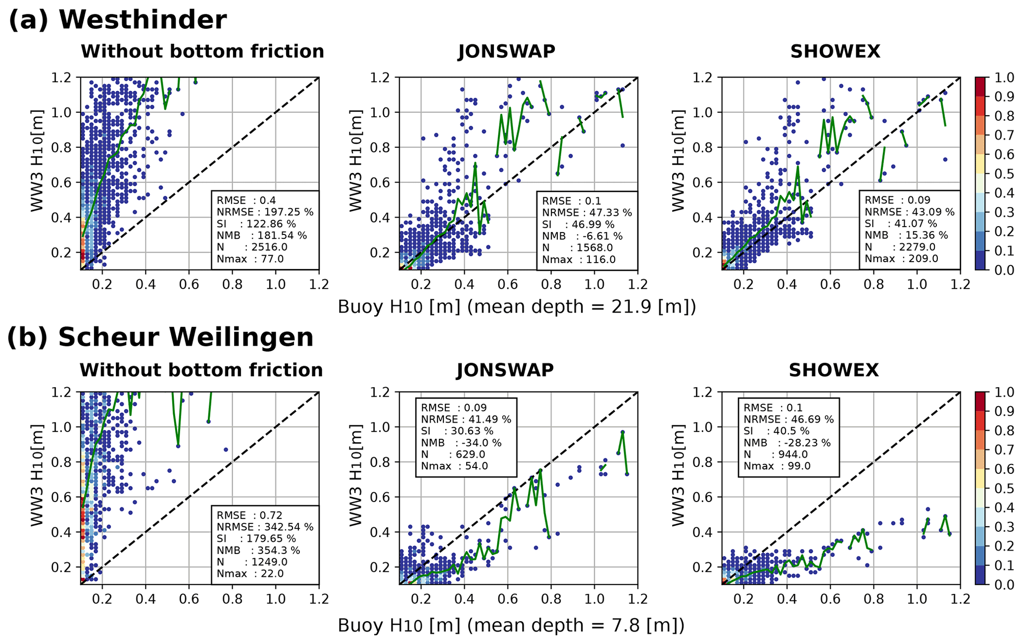
Figure 16 WW3-Buoy H₁₀ comparison for tests without bottom friction, using default JONSWAP and with SHOWEX parameterization including the implemented bottom sediment map. Results for (a) Westhinder and (b) Scheur Wielingen buoy location for the year 2014. Green line shows the modeled averaged values at each 0.02 m wave height bin. Color bars represent the wave height occurrences normalized by the total number of analyzed data N.

6 Model validation with altimetry data

Satellite altimetry provides a unique resource for worldwide wave height measurements. The integration and inter-calibration of past and ongoing missions have allowed us to continuously extend the coverage of measured data in space and time (Ribal and Young, 2019; Dodet et al., 2020). These datasets have been commonly used in open-ocean applications to improve our understanding of the sea states globally. On the other hand, their application in coastal (especially nearshore) areas has been very limited due to increased noise levels in the return signal. What is regarded as noise is actually the detection of the non-Gaussian land surface, which makes it difficult to retrieve the waves' geophysical signal in the radar footprint.

The Sea State CCI V2 dataset employs the WHALES partial waveform retracking algorithm, more effective for reducing the intrinsic noise of the return signal and suitable for coastal applications (Schlembach et al., 2020; Passaro et al., 2021). The vast number of measurements available at distances from the coast lines down to 5 km and less also implies a large coverage of measured wave heights in shallower-depth areas, providing a broader description than local in situ records. Making use of the coverage and improvements in this altimeter product, we analyzed the performance of our mesh over part of the wave hindcast described in Accensi et al. (2021), which was created using the same mesh employed in the present study.

We analyzed three zones of the modeled area: the Bay of Biscay, the North Sea, and the English Channel. The purpose of the defined zones is to assess the performance of the model in different wave generation and propagation conditions. The Bay of Biscay is constantly exposed to swells radiating from the North Atlantic. In the North Sea, wave conditions are dominated by the local winds blowing over a well-defined fetch and partially influenced by the swells from the Norwegian Sea. Finally, in the English Channel, most of the swells' energy arriving from the North Atlantic is blocked, refracted and dissipated at its western end, local waves are generated over a very short fetch, and it is highly influenced by its tidal regime.

Using an along-track comparison of the modeled wave heights with respect to the altimeter-derived wave heights, the bias and scatter were computed per altimeter mission as a function of the distance to the coast, using bins of 1 km and considering wave heights larger than 1 m. To provide an idea of the lower- and upper-bound values of bias and scatter from distances of 1 km offshore up to 80 km, the performance parameters were computed over the complete available years of data per mission until 2018: from 2002 to 2012 for Jason-1 and Envisat, 2008 to 2017 for Jason-2, 2013 to 2018 for Saral, and 2016 to 2018 for Jason-3 (Fig. 17).

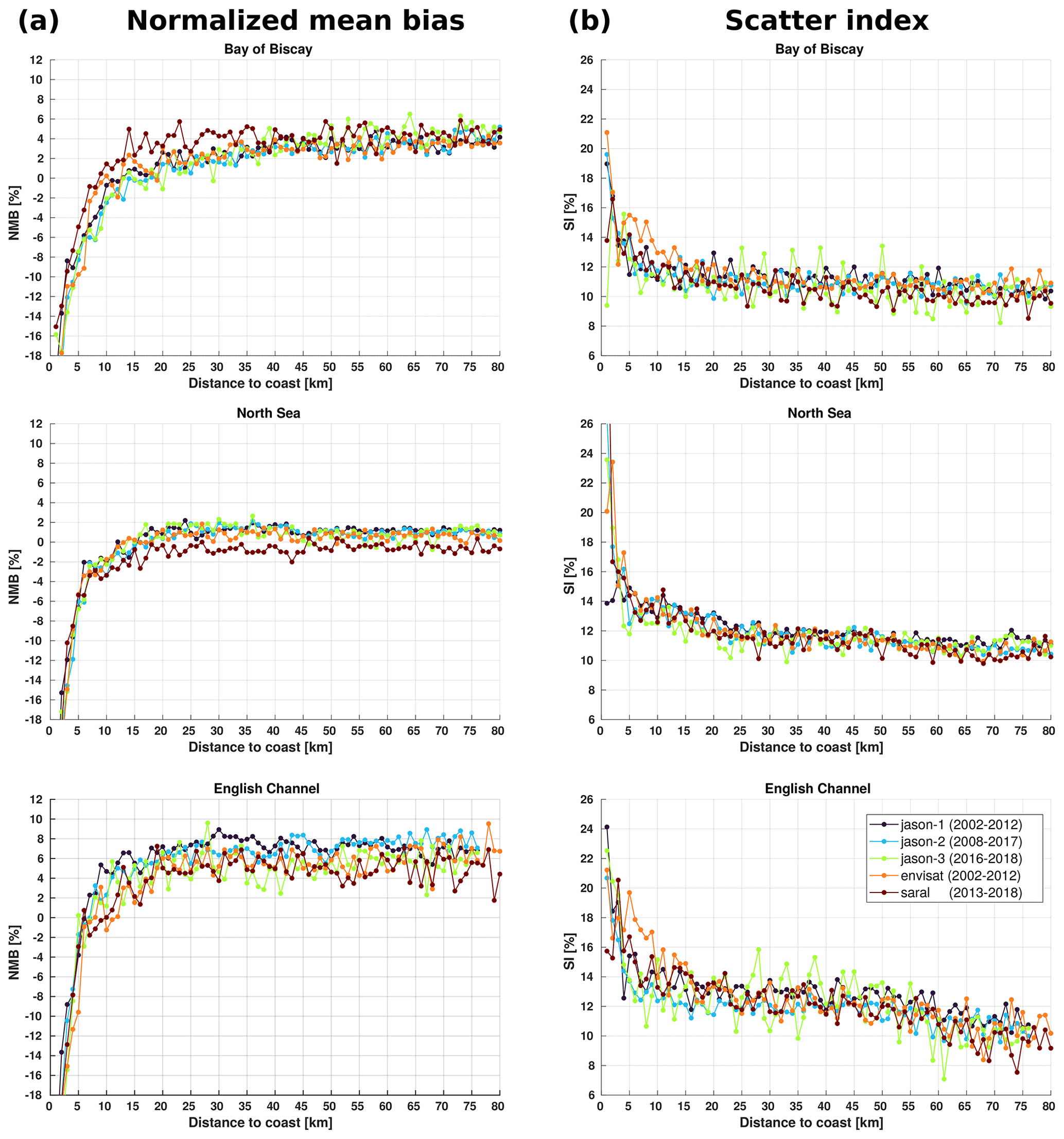
Figure 17 (a) Bias (NMB) and (b) scatter (SI) for wave heights as a function of distance to the coast (WW3 – altimeter wave height). Bin width is 1 km.

From distances to the coast of 15 km and more we noticed a constant positive bias ranging from 2 % to 6 % in the Bay of Biscay and in some cases going up to ∼8 % in the English Channel. In the North Sea, bias changes are more constrained between ±2 % (Fig. 17a). The positive bias in the Bay of Biscay is thought to be related to the BC obtained from the global hindcast using T475, which was calibrated with the Jason-2 data from CCI V1. These data were indeed found to overestimate wave heights recorded by offshore buoy measurements (Dodet et al., 2020), which has been corrected in V2. The English Channel stands out as a high-bias and high-scatter area, which is thought to be caused by the reduced number of valid altimeter measurements in this area and inaccuracies of the forcing fields. Finally, less influenced by the BC and with an extended fetch for wave growth, the North Sea presents the lowest bias values, which along with the lower scatter (Fig. 17b) shows the good performance of the proposed parameterization and model setup in this area.

An overall bias decrease is observed for distances to the coast smaller than 15 km, which implies that in general the wave heights from altimeters are higher than those from the model. These differences are more accentuated particularly in the Bay of Biscay at distances from the coast shorter than 10 km. Even with the higher uncertainty in modeled/measured wave heights closer to the shore, the available altimetry data down to ∼6 km offshore still provide unprecedented access to coastal information that, even at this early stage, allows us to evaluate the model performance.

7 Conclusions

In the present study we investigated the drivers of model errors in coastal areas and how choices of parameterization, forcing, spectral and spatial resolution, and boundary conditions affect the characteristics of the simulated sea states. Extensive sensitivity analyses were carried out with a high-resolution regional wave model for European coastal waters using the WAVEWATCH III framework. The performed tests and analyses aimed to assess when and where the choices in the model setup have a significant effect in regions where wave interactions with complex bathymetry, tidal currents, and bottom roughness become important in wave propagation.

Overall, spatial resolution is one of the most important elements in shallow-depth areas. We found that a higher spatial resolution adequate to solving bathymetry features and explicitly solving coastlines can introduce changes in modeled wave height of about 20 % when compared to lower-resolution global models. Differences become more significant below 400 m depth, in areas where refraction and diffraction are dominant or in regions sheltered from the most frequent swell conditions.

Changes in the energy distribution of the spectrum were analyzed mainly from two points of view, introduced by modifications in the parameterization and due to changes in directional resolution. Modification of the swell dissipation terms did not impact the wave energy distribution in the regional domain significantly, although its effect becomes important at global scales (Alday et al., 2021). In general, the applied enhancement to intensities higher than 21 m s⁻¹ in the ERA5 wind fields improves the model accuracy at swell-exposed locations, helping to reproduce realistic energy levels for frequencies lower than 0.05 Hz, partially solving their otherwise high underestimation (more than −50 % in some cases). These findings suggest that the considerations taken to generate the boundary conditions at a global scale are one of the most important factors on shorelines exposed to waves from the North Atlantic.

Spectral energy differences due to directional-resolution choices are larger than 10 % at frequencies lower than 0.1 Hz. The effect is visible from the boundary to the nearshore in zones influenced by the BC. Differences in wave parameters (SPR, T_p, D_p) observed between model tests suggest that the proper selection of directions to define the BC and within the nested model will help to reduce random errors. It was also found that with 10^∘ resolution, the GSE is successfully alleviated in the mesh.

Within areas with large tidal amplitudes, including tidal forcing (currents and levels) typically changes wave parameters by about 10 % at each output time and locally much more (e.g., Ardhuin et al., 2012). These differences are reduced for H_s and D_p for a monthly average but can still be larger than 5 % for the SPR and T_p. These findings imply that even if the average wave heights might be well estimated without tidal forcing, the propagation and evolution of the wave fields will be different. This can be observed in the H_s and T_m01 time series at buoy 62059 (Fig. 10).

Comparing wave heights retrieved from altimeter data with 1-year simulations, we identified areas influenced by bottom friction dissipation by looking at changes in H_s. We found that these changes can be observed at depths smaller than 50 m. In shallower areas of the North Sea and some sections of the Atlantic coast of France, including the SHOWEX bottom friction parameterization helps to reduce the H_s bias. Comparisons between model and in situ measurements of H₁₀ revealed an underestimation of the wave energy in the low-frequency bands in very shallow areas. This effect could be related to a higher sensitivity of the SHOWEX parameterization in very shallow depths; thus, dissipation induced in longer wave components is overestimated with our current model setup.

Using five available missions from the Sea State CCI V2 dataset we performed a validation of the modeled wave height as a function of the distance to the coast, between the years 2002 to 2018. We observed an overall increase in wave height differences with our model for distances to the coast smaller than 10 km that can reach −8 % (on average) at 5 km from the coast. These differences are likely due to increased uncertainties in altimeter measurements within the last 10 km from the coast, where coastal features are known to strongly impact radar waveforms (Vignudelli et al., 2019).

We found that in many cases time-averaged differences between model setups or with respect to in situ data are small, but these differences can be significant at each output time, implying that the time evolution of the sea states is in fact different. This could partially explain cases with low bias and still larger random errors (e.g., SI) in some locations, when modeled wave parameters are compared with measurements.

Due to the different characteristics of the modeled domain (e.g., bathymetry features, bottom sediment type, fetch, and tidal amplitudes) the factors driving the accuracy of the model cannot be completely generalized. Instead, through the proposed analyses we have identified where changes in the wave field characteristics are more significant with different choices in forcing, resolution, and parameterizations. Yet, it is not straightforward to assess how the combination of these choices can potentially compensate for errors in the simulations. We find that boundary condition effects are most easily evaluated at deep-water or partially sheltered locations (see also Crosby et al., 2017), while separating bottom friction from other effects will require a further analysis of specific swell events.

Appendix A: Detailed model implementation

All simulation results presented were generated using the unstructured grid WAVEWATCH III model version 7.0. The following compilation switches were included:

• physical parameterizations – LN1 ST4 STAB0 NL1 BT4 DB1 MLIM TR0 BS0 REF1 WCOR RWND TIDE

• advection scheme – UQ

• numerical choices – F90 NOGRB NC4 SCRIP SCRIPNC SHRD TRKNC O0 O1 O2 O2a O2b O2c O3 O4 O5 O6 O7.

In our tests, we used a few different combinations of the swell dissipation terms SWELLF7 and SWELLF4 of the ST4 parameterization (Sect. 5.2). Here we present the model namelist with its final values as defined in T475:

• wave growth and swell dissipation (SIN4 namelist) – BETAMAX = 1.75; SWELLF = 0.66; TAUWSHELTER = 0.3; SWELLF3 = 0.022; SWELLF4 = 115000.0; SWELLF7 = 432000.00

• wave reflection parameters (REF1 namelist) – REFCOAST = 0.05; REFCOSPSTRAIGHT = 4; REFFREQ = 1.0; REFMAP = 0.0; REFSLOPE = 0.03; REFSUBGRID = 0.1; REFRMAX = 0.5

• SHOWEX parameterization (SBT4 namelist) – SEDMAPD50 = T; BOTROUGHMIN = 0.0400; BOTROUGHFAC = 1.0

• unstructured grid options (UNST namelist) – UGBCCFL = F; UGOBCAUTO = T; UGOBCDEPTH = −15.0; EXPFSN = T

• wind correction and others (MISC namelist) – NOSW = 6; WCOR1= 21; WCOR2=1.05.