the Creative Commons Attribution 4.0 License.
the Creative Commons Attribution 4.0 License.
 | 22 Nov 2022
Seasonal variation in eddy activity and associated heat/salt transport in the Bay of Bengal based on satellite, Argo, and 3D reprocessed data
Jie Zhang
Based on satellite altimetry data spanning over 26 years in combination with Argo profile data or three-dimensional (3D) reprocessed thermohaline fields, the eddy synthesis method was used to construct vertical temperature and salinity structures of eddies in the Bay of Bengal, and the seasonal thermohaline properties of eddies and the heat and salt transport by eddies were analyzed. Analysis revealed that mesoscale eddy activities and the vertical thermohaline structures in the Bay of Bengal have evident seasonal variation. Temperature anomalies caused by eddies are usually between ±1 and ±3 ∘C (positive for anticyclonic eddies (AEs) and negative for cyclonic eddies (CEs)), and the magnitude varies seasonally. Salinity anomalies caused by eddies are small and disturbance signals in the southern bay due to the small vertical gradient of salinity there; salinity anomalies in the northern bay are generally between ±0.2 and ±0.3 psu, negative for AEs and positive for CEs. Owing to seasonal changes in both the eddy activity and the vertical thermohaline structure in the Bay of Bengal, the eddy-induced heat and salt transport in different seasons also changes substantially. Generally, high heat and salt transport is concentrated in eddy-rich regions, e.g., the western, northwestern, and eastern parts of the bay, the seas to the east of Sri Lanka, and the region to the southeast outside of the bay. The southern part of the bay shows weak salt transport owing to the inconsistent salinity signal within eddies. The result of the divergence of eddy heat transport illustrates that the 10–20 W m−2 value of the eddy-induced heat flux is comparable in magnitude with the annual mean air–sea net heat flux in the Bay of Bengal. Compared with the large-scale net heat flux and freshwater flux at the surface, the eddy-induced heat/freshwater transport can contribute substantially to regional and basin-scale heat/freshwater variability. This work provides data that could support further research on the heat and salt balance of the entire Bay of Bengal.
- Article
(21247 KB) - Full-text XML
-
Supplement
(1360 KB) - BibTeX
- EndNote


Oceanic mesoscale eddies are rotating coherent structures of ocean currents, which generally refer to ocean features with spatial scales from tens to hundreds of kilometers and timescales from days to months (Robinson, 2010). Following recent advances in remote-sensing satellites and the abundance of in situ observational data, it has been established that mesoscale eddies can be found nearly everywhere in the world's oceans (Chelton et al., 2011a; Xu et al., 2011; Fu, 2009; Chaigneau et al., 2009), and they transport water, heat, salt, and other tracer materials as they propagate in the ocean, impacting water column properties and biological activities (Chelton et al., 2011b; Xu et al., 2011; Dong et al., 2014). Combining altimetry data with Argo profile data, Zhang et al. (2014) found that mesoscale eddies have strong zonal mass transport which was comparable in magnitude to that of the large-scale wind- and thermohaline-driven circulation.
The Bay of Bengal is located in the northeastern part of the Indian Ocean. The northern Indian Ocean is subject to monsoonal wind forcing, which means there is a near-complete reversal of winds from summer (the Southwest Monsoon) to winter (the Northeast Monsoon), and the ocean circulation responds accordingly. During the summer Southwest Monsoon, the upper-ocean circulation from south of the Equator to the northern boundary is eastward. The eastward flow around southern India is called the Southwest Monsoon Current (SMC). During the winter Northeast Monsoon, a westward flow, the Northeast Monsoon Current (NMC), appears along the south side of Sri Lanka and India. Affected by complex exogenous effects such as the local monsoon, equatorial remote forcing, and seasonal changes in river runoff, the circulation of the Bay of Bengal has obvious seasonal variation (Hacker et al., 1998; Eigenheer and Quadfasel, 2000; Somayajulu et al., 2003; Qiu et al., 2007; Cheng et al., 2013; Chen et al., 2017). The climatological monthly mean circulation structure and thermohaline properties of the Bay of Bengal are shown in Fig. 1. During the summer Southwest Monsoon, alternate cyclonic and anticyclonic circulation cells prevail in the western bay; a basin-scale cyclone-like gyre dominates the bay during the November monsoon transition; during the winter Northeast Monsoon, the cyclonic gyre weakens, and an anticyclonic circulation appears in the northern bay; in spring premonsoon, the bay is again dominated by a strong anticyclonic gyre. The East Indian Coastal Current (EICC), i.e., the western boundary current in the Bay of Bengal, reverses direction twice a year, flowing northeastward in the Southwest Monsoon and southwestward in the Northeast Monsoon.
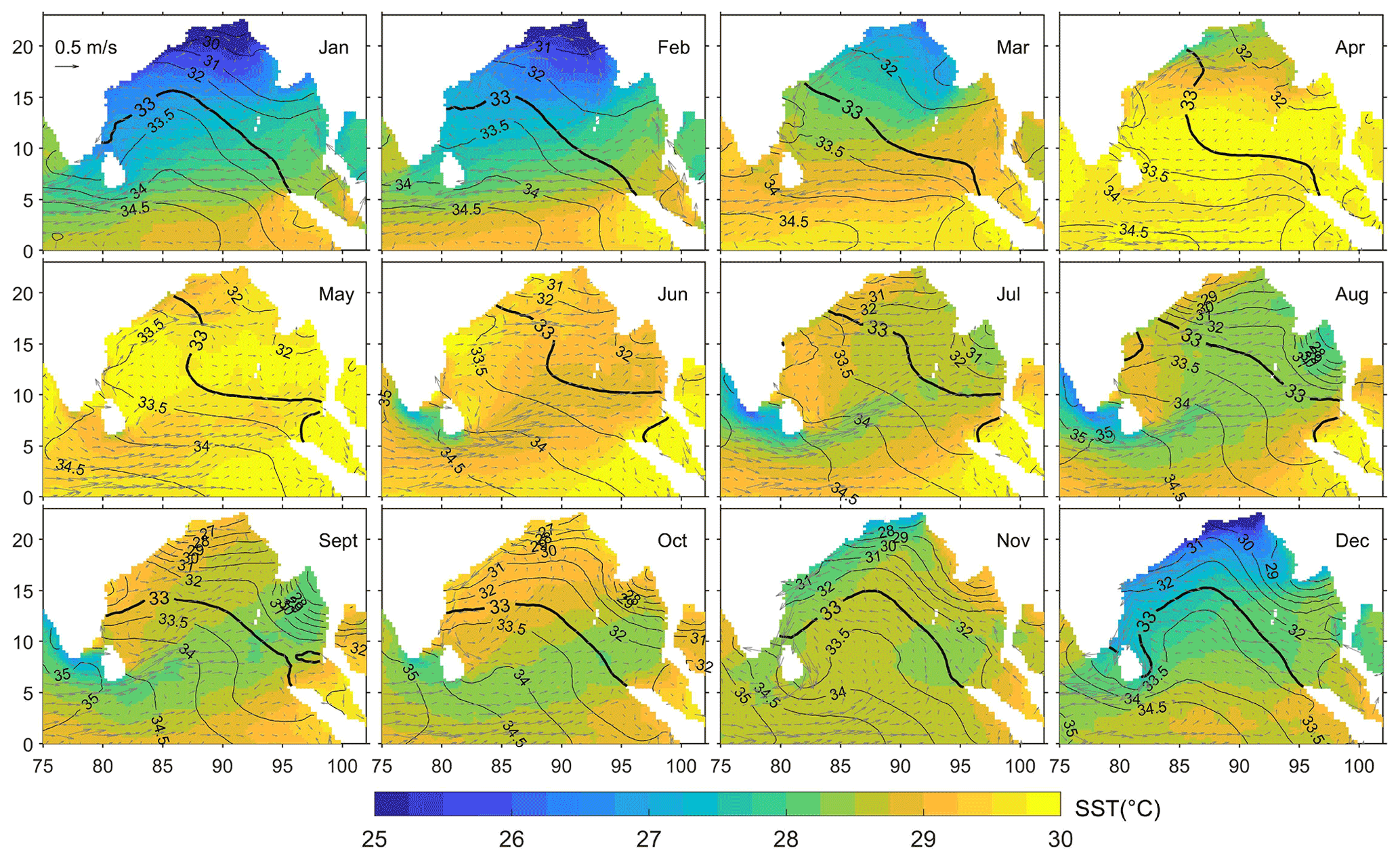
Figure 1Climatological monthly sea surface temperature fields (color), mean surface currents (arrows), and surface salinity (contours) in the Bay of Bengal. The climatological sea surface temperature fields are from the monthly averaged OISST dataset with a 0.25∘ regular grid at global scale from January 1982 to December 2011 (Banzon et al., 2014; ftp://eclipse.ncdc.noaa.gov/pub/OI-daily-v2/, last access: 8 April 2022). The climatological surface currents are from the monthly averaged global total velocity field (MULTIOBS_GLO_PHY_REP_015_004) at 0 and 15 m with a 0.25∘ grid from January 1993 to December 2018 (Etienne, 2018). The climatological surface salinity fields are from the global SSS/SSD L4 reprocessed dataset (MULTIOBS_GLO_PHY_REP_015_002) with a 0.25∘ grid from January 1993 to December 2018 (Mertz et al., 2018). The latter two datasets are available at http://marine.copernicus.eu (last access: 12 August 2021).
The sea surface temperature (SST) in the Bay of Bengal has obvious seasonal variation, which is influenced by the inflows from the tropical Indian Ocean and Arabian Sea to the south, considerable river runoff to the north, and abundant precipitation (Graham and Barnett, 1987; Rao et al., 2002; Shenoi et al., 2002; Murty et al., 1998). A cold pool exists to the southern Bay of Bengal and around Sri Lanka during the summer Southwest Monsoon, maintained by the advection and entrainment of cooler water by the SMC in spite of the ocean gaining heat from the atmosphere (Das et al., 2016; Vinayachandran et al., 2020). The salinity in the Bay of Bengal decreases from about 34 psu at about 5∘ N to 30 psu or less in the north. The Bay of Bengal with the fresh waters is dominated by the considerable runoff from all of the major rivers of India, Bangladesh, and Burma (Varkey et al.,1996; Prasad, 1997; Rao et al., 2003). The seasonal barrier layer in the Bay of Bengal is brought about by the strong salinity stratification due to the influx of freshwater from river discharge and excess precipitation over evaporation (Kumari et al., 2018; Vinayachandran et al., 2002; Akhil et al., 2014).
Many studies show that there are abundant cyclonic (CEs) and anticyclonic eddies (AEs) associated with the seasonally circulations in the Bay of Bengal (Babu et al., 1991; Prasanna Kumar et al., 2004; Chen et al., 2012, 2018; Cui et al., 2016; Cheng et al., 2018). Somayajulu et al. (2003) analyzed the seasonal and inter-annual variability of surface circulation in the Bay of Bengal and found that the monsoon conversion, EICC instability, and the coastally trapped Kelvin waves and radiated Rossby waves are responsible for the observed variability of the mesoscale eddies in the bay. Chen et al. (2018) suggested that both local monsoonal winds and remote equatorial winds as well as ocean internal instability are the main reasons for the generation and modulation of eddy kinetic energy in this region. The upper seasonal circulation in the Bay of Bengal is driven by the monsoon, on which are superimposed the local Ekman drifting and geostrophic circulation, so its seasonal changes are not completely synchronized with the monsoon transition (Vinayachandran et al., 1999; Qiu et al., 2007; Sreenivas et al., 2012).
The surface characteristics of oceanic eddies can be inferred from remote-sensing data, and the vertical thermohaline profile of subsurface waters can be provided by Argo buoys. In recent years, by combining satellite altimetry and Argo profiling float data, analysis of the vertical structure of eddies has become an important part of the study of oceanic eddies (Chaigneau et al., 2011; Yang et al., 2013; Amores et al., 2017). Knowledge of the vertical structure of the ocean is vital both for comprehensive understanding of ocean dynamic processes and for analysis of the ocean circulation and energy transport. Based on satellite altimetry and Argo floats, Lin et al. (2019) and Gulakaram et al. (2020) showed that eddy-induced ocean anomalies in the Bay of Bengal are mainly confined to the upper 300 m and eddy thermohaline structure has a seasonal character. Cui et al. (2021) found that the thermohaline properties of mesoscale eddies in the Bay of Bengal are different in the north–south direction. Combining estimated eddy diffusivity from 25 years of altimetry data with corresponding tracer gradients from the World Ocean Atlas 2013, Gonaduwage et al. (2019) investigated the meridional and zonal eddy-induced heat and salt transport in the Bay of Bengal, and they found that the baroclinic instability, local wind-stress curl, and remote forcing from the Equator contribute to the seasonal modulation of eddy-induced heat transport.
Many studies examined the surface characteristics of eddies in the Bay of Bengal, and some have investigated the vertical eddy properties (Nuncio and Kumar, 2012; Dandapat and Chakraborty, 2016; Chen et al., 2012, 2018; Cui et al., 2021). However, few studies considered the seasonal variation in the three-dimensional (3D) thermohaline structure and the heat and salt transport due to mesoscale eddies. Considering the hydrological differences from north of the bay to the south, the eddy vertical structure in different subregions should be further studied. Owing to the characteristics of the oceanic circulation and regional monsoons, the eddy activity in the Bay of Bengal has obvious seasonal differences. Specifically, the seasonal variation in surface eddies, 3D thermohaline structure of eddies and its regional variation, seasonal heat/salt transport, and their spatial distribution characteristics have not been analyzed comprehensively.
In this study, based on merged satellite altimetry data spanning over 26 years, the automatic identification method was used to extract information on the position and shape of mesoscale eddies in the Bay of Bengal, and the seasonal variation in the eddies was analyzed in detail. Then, by combining the satellite altimetry data with either Argo profile data or 3D thermohaline fields, the eddy synthesis method was used to construct the 3D thermohaline structures of eddies in the study area, and their seasonal thermohaline properties and regional thermohaline variations were analyzed. Finally, based on eddy movement and thermohaline properties, the heat and salt transports by eddies were estimated, and their seasonal variation and spatial distribution characteristics were analyzed. The remainder of this paper is organized as follows. Section 2 describes the data and methods adopted in the study. Section 3 presents the seasonal variations and seasonal 3D thermohaline properties of the eddies. Section 4 analyzes the seasonal heat and salt transports by eddies in the Bay of Bengal. Finally, summary and discussion are presented in Sect. 5.
2.1 Data
The daily and monthly gridded sea level anomaly (SLA) products (SEALEVEL_GLO_PHY_L4_REP _OBSERVATION_008_47) from January 1993 to February 2019 are used to determine the presence and positions of mesoscale eddies in the Bay of Bengal. The SLA product is processed by the Archiving, Validation, and Interpretation of Satellite Oceanographic data (AVISO) and distributed by the European Copernicus Marine Environment Monitoring Service (CMEMS, http://marine.copernicus.eu, last access: 12 August 2021).
The Argo float profiles provided by the Coriolis Global Data Acquisition Center of France (http://www.coriolis.eu.org, last access: 3 May 2022) are used to analyze the vertical temperature and salinity structures of eddies. In the analysis, we have taken pressure, temperature, and salinity profiles with quality flag 1 and have followed Chaigneau et al. (2011) for the selection of the profiles from the year 2001 to 2019. The final dataset includes a total of 29 219 available profiles in our study region. Potential temperature θ and salinity S data in each profile were linearly interpolated onto 101 vertical levels from the surface to 1000 dbar with an interval of 10 dbar using the Akima spline method. To get the thermohaline structures of mesoscale eddies, potential temperature anomaly θ′ and salinity anomaly S′ of Argo profiles were computed by removing Argo seasonal-mean climatologic profiles.
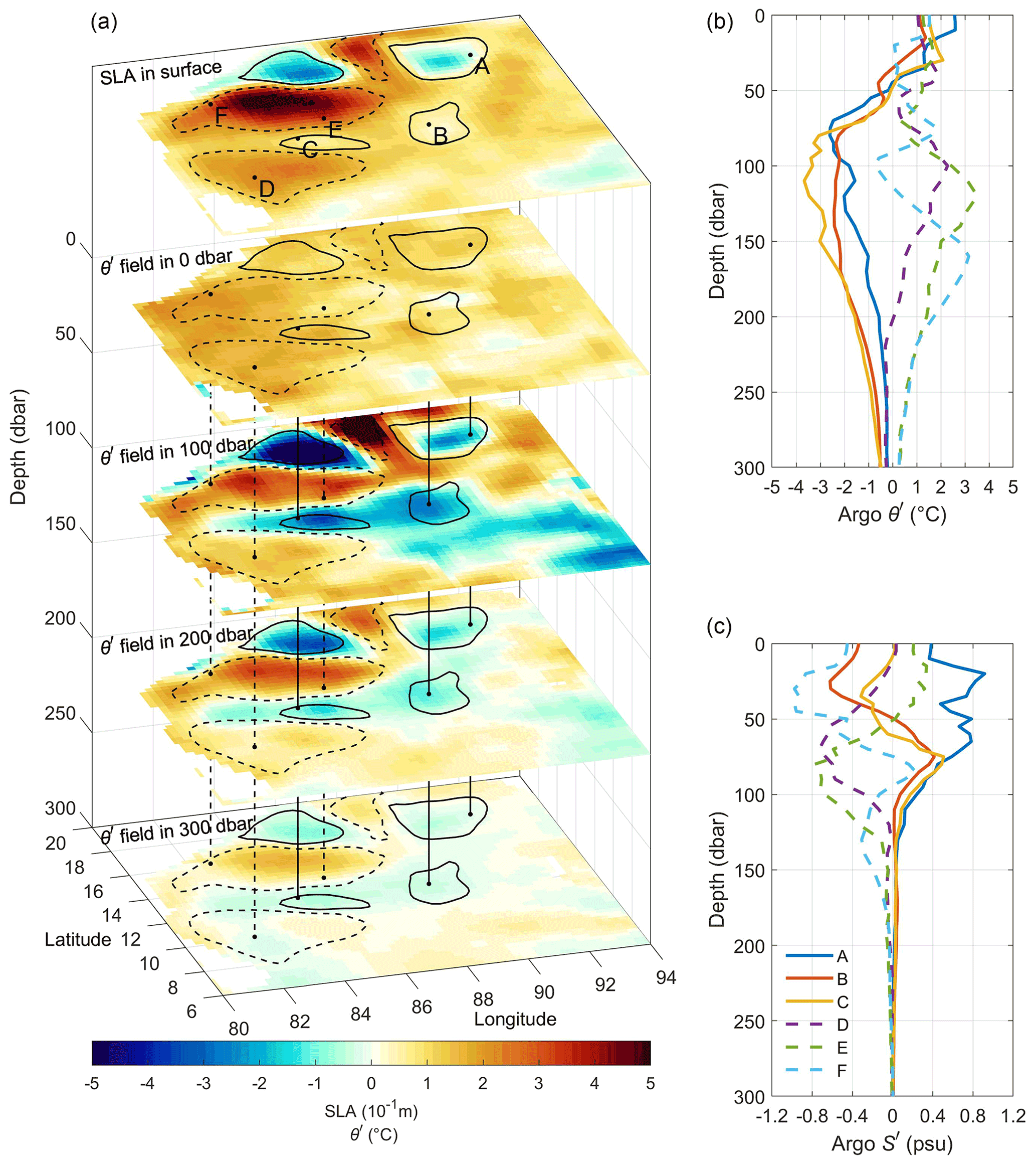
Figure 2(a) A case of matching identified eddies from sea level anomaly (SLA) fields with vertical temperature anomaly θ′ and salinity anomaly S′ fields on 20 May 2017. The top layer represents the SLA fields and identified eddies, where solid and dashed lines represent cyclones (CEs) and anticyclones (AEs), respectively. The colors in the lower layers represent the temperature anomaly θ′ field at different depths from the ARMOR3D data. The vertical solid and dashed lines represent Argo profiles located in CEs and AEs, respectively, and each profile is marked by a letter (A–F) in the top layer. (b, c) The graphs on the right show the vertical temperature and salinity anomaly profiles of the Argo buoy (A–F) located in the eddies.
The ocean reprocessed data can provide the 3D thermohaline information of the surface eddies captured by the satellite altimetry. The Global ARMOR3D L4 reprocessed dataset (MULTIOBS_GLO_PHY_REP_015_002, distributed by CMEMS, http://marine.copernicus.eu, last access: 12 March 2022) consists of 3D temperature, salinity, heights, and geostrophic currents, available on a 0.25∘ regular grid and at 33 depth levels from the surface down to the bottom (Guinehut et al., 2012). The ARMOR3D dataset is obtained by combining satellite (SLA, geostrophic surface currents, SST) and in situ (temperature and salinity profiles) observations through statistical methods. The dataset is available as weekly means for the period 1993–2019. Similar to Argo profiles, the 3D temperature and salinity anomaly fields were computed by removing ARMOR3D seasonal-mean climatologic fields.
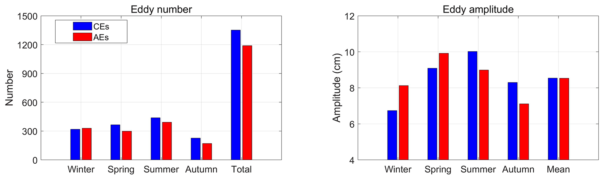
Figure 3The eddy number and amplitude of monthly cyclones (CEs) and anticyclones (AEs) in different seasons based on monthly averaged sea level anomaly fields from January 1993 to February 2019 in the Bay of Bengal.
2.2 Eddy detection, 3D reconstruction, and heat–salt transport estimation
2.2.1 SLA-based eddy identification and tracking
In SLA fields, mesoscale eddies can generally be identified as regions enclosed by SLA contours. A geometric algorithm for eddy identification based on the outermost closed contour of an SLA has been proposed by Chelton et al. (2011a). Following the algorithm, an eddy is defined as a simply connected set of pixel grids that satisfy some criteria. For the Bay of Bengal, the minimum amplitude of an eddy is increased from the original 1 cm used by Chelton et al. (2011a) to 3 cm in this study. The reason for this change is that the accuracy of measuring heights using Jason series altimeters (including TOPEX/Poseidon and Jason-1/2/3), which currently have optimal performance for observing ocean dynamics, is only about 2 cm in the open sea (Dufauet al., 2016). Furthermore, the distance between the two furthest apart internal points in an eddy is less than 600 km for avoiding enclosed elongated regions.
Based on daily SLA fields, the mesoscale eddies in the Bay of Bengal are identified, and the eddy amplitude, eddy scale/radius, and eddy propagation velocity are quantified over the study area. The eddy amplitude is defined here to be the magnitude of the SLA difference between the eddy boundary and the eddy center (local extremum). The eddy scale/radius is defined as the equivalent radius of a circle with the same area which is delimited by the eddy boundary. Based on the eddy identification results in the continuous time series, the evolution process of eddies (eddy trajectories) in the ocean can be tracked by comparing the eddy positions and dynamic properties (Chaigneau et al., 2008; Henson and Thomas, 2008; Nencioli et al., 2010; Souza et al., 2011). For an eddy at day n, its trajectory is tracked by searching the most similar eddy at the subsequent day n+1 in terms of the type and eddy characteristics within a circle of eddy radius (Chaigneau et al., 2008; Cui et al., 2021). To avoid the false tracking of the eddies, the same eddy is searched continuously for 10 d with circles of growing radius (maximum double eddy radius on the 10th day) when no match eddy is detected in subsequent time step n+1. The lifetime of an eddy represents the duration of an eddy from its generation to its termination. The eddy propagation velocity is defined as the change in the eddy center position as a function of time.
In addition, in order to study the seasonal spatial distribution of eddies, monthly eddies are identified from the monthly SLA fields without trajectory tracking. For such monthly eddies, the tracking processing is not performed, and the monthly results identified from monthly SLA fields are processed as individual eddies.
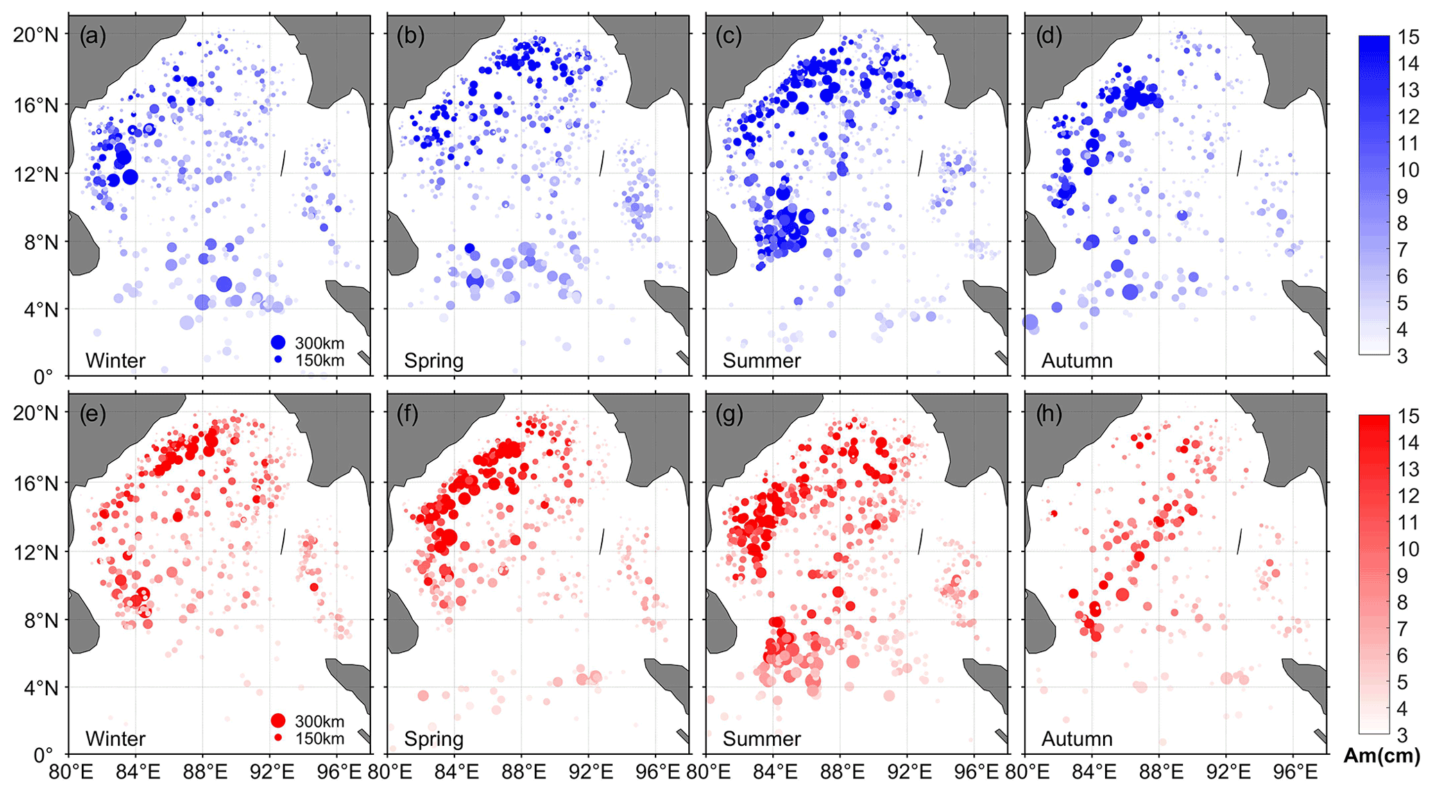
Figure 4Seasonal spatial distribution of monthly cyclonic eddies (CEs, upper) and anticyclonic eddies (AEs, lower) based on monthly averaged sea level anomaly fields from January 1993 to February 2019 in the Bay of Bengal. Blue and red points represent CEs and AEs, respectively, where the color intensity represents the eddy amplitude (Am; unit: cm) and the size of the point represents eddy scale (radius).
2.2.2 3D eddy reconstruction
Combined with the satellite altimetry data and the Argo profiles, composite 3D structures of a single CE and a single AE were created based on the eddy synthesis method in the study. The 3D structures of eddies were constructed by surfacing the Argo float profiles into SLA-based eddy areas, as shown in Fig. 2. We considered the detection results (from daily SLA fields) of the long-lived eddy (eddy trajectories with a lifetime ≥30 d) to match the Argo profiles on the same day, and selected Argo profiles with a distance of <1.5 radii from the eddy center for vertical eddy structure analysis. By matching identified eddies with Argo profiles in a long time (from the year 2001 to 2019), a large number of Argo profiles within eddies can be obtained. Consequently, 3882 and 4097 Argo profiles were selected for cyclonic and anticyclonic eddy reconstruction, respectively. These Argo profiles were interpolated to create an average CE and an average AE 3D profile. Due to Argo profiles captured by eddies being scattered (spatially nonuniform), it is necessary to transform these Argo profiles into a unified eddy center coordinate, so as to combine the vertical temperature and salt information provided by all profiles to obtain the 3D thermohaline structures of the composite eddy. Specifically, for each Argo profile matched by an eddy, we calculated the relative zonal and meridional distances to the eddy center. The relative distances were normalized relative to the eddy radius (nondimensionalization). Then, all the Argo profiles were transformed into the normalized eddy coordinate space, and θ, S and θ′, S′ data of Argo profiles were mapped onto a 0.1×0.1 grid using inverse distance weighting interpolation at each vertical level from the surface to 1000 dbar. Finally, composites of 3D thermohaline structures were reconstructed in each normalized grid location. Considering the hydrological differences from north of the bay to the south, here the Bay of Bengal is divided into north and south subregions with 12∘ N as the boundary to study the eddy 3D structure of each subregion. The Argo profiles acquired within eddies were classified according to season, so the 3D structures of eddies were reconstructed in different seasons.
Since the Argo floats only provide one-dimensional information on the profile and Argo profiles are scattered, we can only reconstruct one 3D thermohaline structure of eddies in a region by the above method. The ocean reprocessed data provide the 3D temperature and salinity field data covering the entire space. This allows us to obtain the 3D thermohaline structure of the surface eddies captured by the satellite altimetry by matching the eddy results with the reprocessed 3D field data. Here, the weekly ARMOR3D reprocessed dataset was used to provide vertical structure information on the surface eddies. We matched the eddy results identified from daily SLA fields with the weekly 3D field data at the closest time such that we could obtain the 3D temperature and salt structure of each eddy (Fig. 2a). Similar to the handling of Argo profiles, all eddies were classified by season, and the 3D structures of all vortices in a season were averaged and used for comparison with the reconstruction results of Argo profiles.
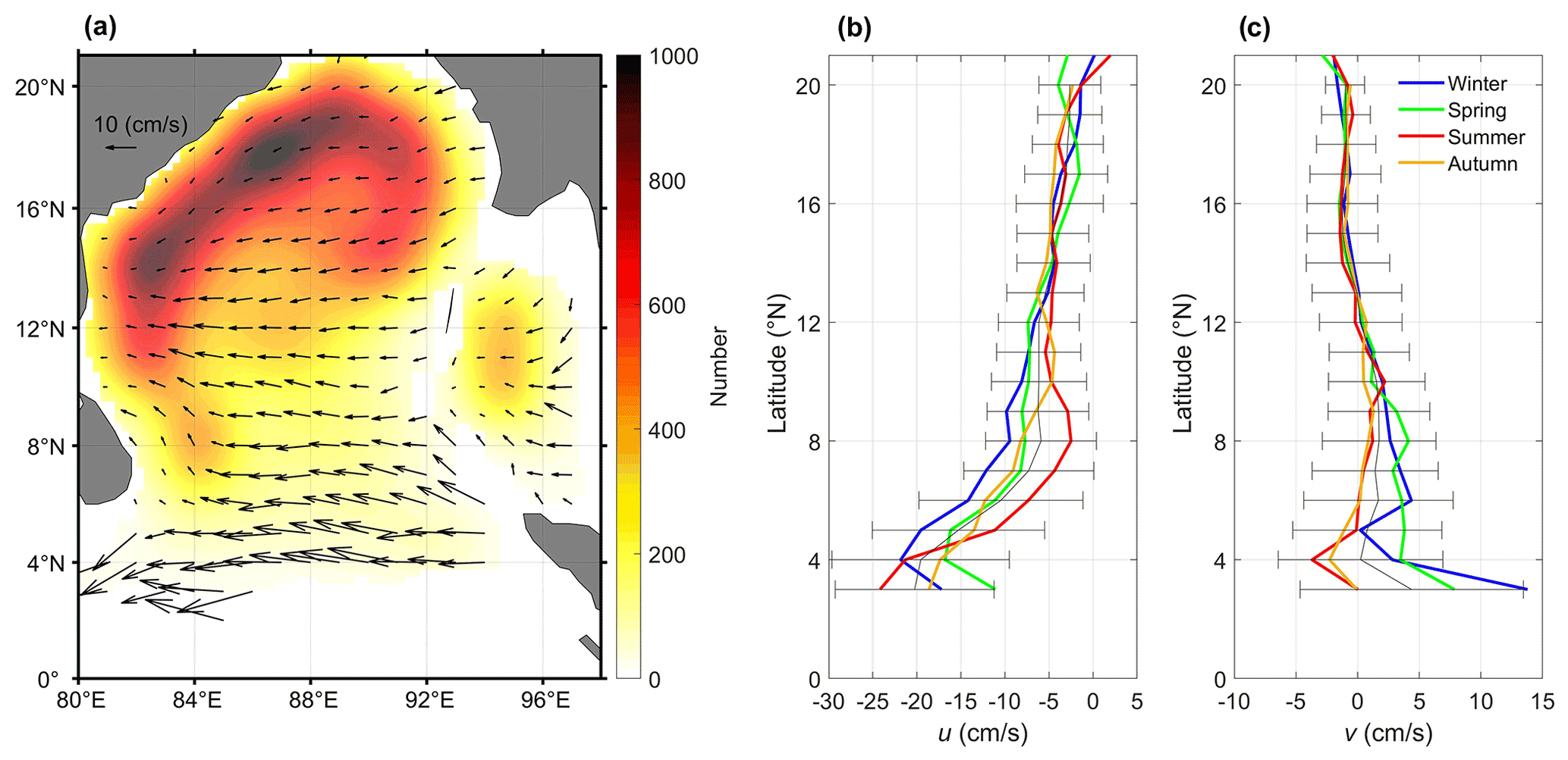
Figure 5(a) Statistical eddy propagation speed (color indicates the numbers of eddy interiors for eddy trajectories with lifetimes ≥30 d that passed through each region) and (b) the zonal component u and (c) the meridional component v (thin solid line represents the mean value and its standard deviation, and the color represents the season) in the Bay of Bengal based on daily SLA fields spanning a 26-year period from January 1993 to February 2019.
2.2.3 Eddy-induced heat and salt transport estimation
A nonlinear eddy can maintain its own waterbody characteristics and have minimal exchange with the surrounding water mass as it propagates in an ocean. By combining the spatial-scale information of the eddies provided by the SLA fields with the vertical temperature and salt anomaly information provided by the ARMOR3D temperature and salinity fields, the heat anomaly He and salt anomaly Se could be obtained for each eddy (the subscript e means eddy):
Here, the mean upper-ocean density and heat capacity are ρ0=1025 kg m−3 and Cp0=4200 J kg−1 ∘C−1. R is the eddy region, D0 is the integration depth (500 dbar for He and 300 dbar for Se; Lin et al. (2019); Gulakaram et al. (2020); also, Sect. 3.2), x and y represent horizontal position, and z represents the vertical depth. The unit of eddy heat anomaly He is joule, and that of salt anomaly Se is kilogram.
Instead of using eddy propagation velocity to calculate eddies' heat transport (Dong et al., 2014), eddy trajectories are used to calculate transport by eddy movements (Dong et al., 2017). Here we use 0.25∘ grid cells to calculate the eddy-induced heat and salt transport through following the eddy trajectory and check whether it crosses grid cell boundaries. If an eddy crosses the west or east boundary, it results in zonal transport, whereas eddy crossing of the north or south boundary results in meridional transport. In addition, the east and the north transport are defined as positive, while the west and the south are negative. For a grid cell, the zonal heat and salt transport Qhz and Qsz (the subscript z means zonal) are equal to the sum of heat anomalies He and salt anomalies Se of all eddies i which cross the east or west boundary, divided by the meridional length Dm of the grid (the subscript m means meridional; unit: m) and time length T (unit: s) (Dong et al., 2017):
Here the unit of heat transport Qhz is W m−1, and that of salt transport Qsz is kg m−1 s−1. The time length T is 26 years corresponding to the time series length of SLA products used for the eddy identification from January 1993 to February 2019. The denominator factor of 2 is because we separately considered the east and west boundaries of the eddy moving through the grid. Similarly, the eddy-induced meridional heat and salt transport Qhm and Qsm are calculated by
Here, Dz is the zonal length of the grid. In the actual calculation, a moving average filter with a box size is applied to reduce noise.
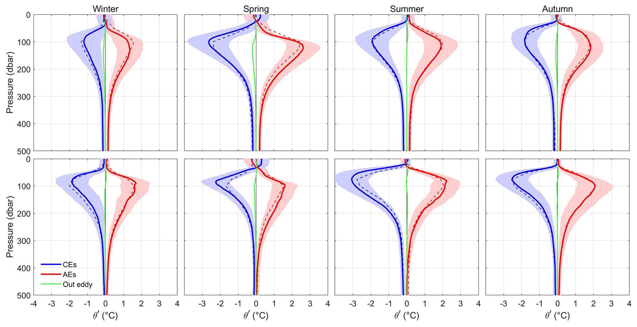
Figure 6Mean vertical profiles of the potential temperature anomaly θ′ of composite cyclonic eddies (CEs, blue lines) and anticyclonic eddies (AEs, red lines) in different seasons for the northern (upper) and southern (lower) bay. The green lines indicate the mean anomalies that were computed from Argo profiles outside eddies relative to the Argo seasonal-mean climatologic profiles. The solid lines indicate the mean anomalies from Argo profiles, the shading indicates the range of 1 standard deviation, and the dashed lines indicate the mean anomalies from the weekly ARMOR3D temperature and salinity field data.
3.1 Seasonal spatial distribution of eddies
The Bay of Bengal is affected by the Southwest Monsoon and Northeast Monsoon, and its entire circulation system is characterized by monsoon circulation. Following many studies on the Bay of Bengal (Somayajulu et al., 2003; Patnaik et al., 2014; Seo et al., 2019), the seasons are defined as the winter monsoon (December–February), spring premonsoon (March–May), summer monsoon (June–September), and autumn postmonsoon (October–November) in the present study. Based on daily SLA fields spanning over 26 years (from January 1993 to February 2019), 620 cyclonic eddies (CEs) and 516 anticyclonic eddies (AEs) (eddy trajectories) with lifetimes ≥30 d in the Bay of Bengal were detected in the eddy tracking procedure. The seasonal distributions of eddy trajectories (Fig. S1 in the Supplement) show that eddy activities have obvious seasonal variation, but messy trajectories obscure the distribution characteristics.
In order to understand the seasonal distribution characteristics of eddies in the Bay of Bengal more intuitively, we used monthly averaged SLA fields to identify eddies that occur frequently in certain regions (here we call them “the monthly eddies”). For such monthly eddies, the tracking processing is not performed, and these monthly results identified from monthly SLA fields are processed as individual eddies. Each individual monthly eddy is counted as one eddy. As a result, a total of 1351 CEs and 1190 AEs (individual monthly eddies) were identified from the monthly SLA fields in the whole Bay of Bengal (Fig. 3). The monthly eddies have a greater number in summer and a smaller number in autumn. Statistically, the mean amplitudes of CEs and AEs are both about 8.3 cm, but they vary greatly in different seasons. Eddy amplitudes are higher in spring and summer than in autumn and winter, especially for AEs in spring and CEs in summer, the mean amplitudes of which are close to 10 cm. Seasonal changes in eddy amplitude illustrate that eddy activities are vigorous in spring and summer and relatively weak in winter and autumn. Based on these monthly eddy results, eddies are classified according to different seasons, and the seasonal spatial distributions of CEs and AEs are given in Fig. 4.

It can be seen from Fig. 4 that CEs and AEs have obvious seasonal variation in their local distribution characteristics. In the winter monsoon season (Fig. 4a and e), although eddies are distributed throughout the Bay of Bengal, many CEs with high amplitude and large radius are clustered in western parts of the bay, while many high-amplitude AEs are clustered in northern parts. The monthly averaged SLA fields (Fig. S3) indicate that the bay is dominated by a cyclonic gyre in December, accompanied by abundant CEs in the western bay. Meanwhile, a persistent AE forms in the northern portion of the bay in January. In the low-latitude equatorial regions, some low-amplitude large-scale CEs often appear in the western waters of Sumatra, are largely manifestations of Rossby waves, and move gradually westward or northwestward with the westward drift of the monsoon (Fig. S1). In the spring premonsoon season, a basin-scale anticyclonic gyre appears and dominates the bay. Within the anticyclonic gyre, AEs are clustered in western and northwestern parts, while some small but high-strength CEs are clustered in the northernmost and western parts of the bay (Fig. 4b and f). Owing to river runoff and coastal current baroclinic instability, cyclonic structures are prone to appear in the northernmost part of the bay (Patnaik et al., 2014; Babu et al., 2003; Kumar and Chakraborty, 2011). In the summer monsoon season, the EICC becomes variable. In western parts of the bay, some persistent CEs often appear on the northern side of the EICC, while AEs are often shed on its southern side (Fig. 4c and g). In addition, many CEs and AEs are clustered in the eastern and northeastern parts of the bay, which are mainly driven by equatorial zonal winds, with both nonlinearity and coastline topography (Cheng et al., 2018). It is noteworthy that a large number of high-amplitude CEs (this refers to the Sri Lanka Dome, Vinayachandran and Yamagata, 1998) are clustered in the eastern seas of Sri Lanka in the summer monsoon season, while corresponding AEs often appear in the south. In the autumn postmonsoon season, a basin-scale cyclonic gyre is formed throughout the entire bay. Together with the southwestward EICC, many CEs appear in northwestern and western parts of the bay, whereas there are few AEs (Fig. 4d and h). In addition, in the central bay, some AEs often appear accompanied by local current variations.
The heat and salt transport efficiencies of mesoscale eddies are related closely to eddy propagation speed (Dong et al., 2014; Gonaduwage et al., 2019; Stammer, 1998). In order to study the propagation direction and speed of mesoscale eddies in the Bay of Bengal, all eddy trajectories with a lifetime ≥30 d from daily SLA fields are analyzed here. The average speed of propagation of eddies in the Bay of Bengal is shown in Fig. 5. In general, eddies move slowly in the western and northern parts of the bay and move faster in central and southern parts. The zonal component u of eddy propagation speed (Fig. 5b) shows that the westward speed of eddies gradually increases from <5 cm s−1 in the north to up to 20 cm s−1 in low-latitude equatorial regions. In addition, eddy propagation speeds clearly bounded by the 12∘ N line of latitude; eddies to the north/south move westward and slightly southward/northward. In terms of the meridional component v of eddy propagation speed (Fig. 5c), the value to the north of 12∘ N is generally negative (southward), while v to the south of 12∘ N is largely positive (northward). The eddy propagation speed in different seasons also shows some differences. The westward speed of eddies is fastest in winter, followed by spring and autumn, and slowest in summer (Fig. 5b). The meridional speed of eddies is faster in winter and spring than in summer and autumn, and eddies move southward outside the bay in summer and autumn (Fig. 5c). The seasonal propagation speed of eddies may be related to the seasonal variation in the overall circulation, especially in the southern part of the bay to the south of 12∘ N. In winter, the background current is westward/southwestward, which is more conducive to the westward propagation of eddies; while in summer, the drifting intrusion of the Southwest Monsoon Current blocks the westward movement of eddies.
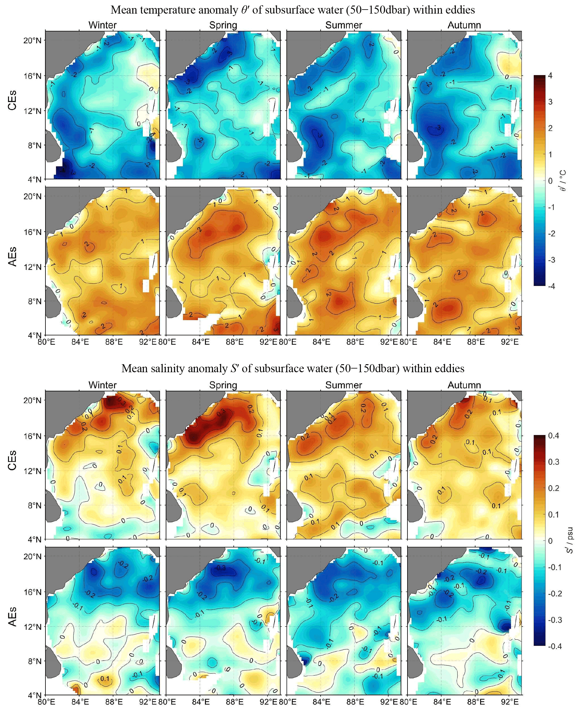
Figure 8Spatial characteristics of the vertical temperature and salinity anomalies of cyclonic eddies (CEs) and anticyclonic eddies (AEs) in the Bay of Bengal in different seasons based on the weekly ARMOR3D temperature and salinity field data.
3.2 Seasonal variation in vertical thermohaline structure of eddies
To reveal the seasonal variation in the vertical thermohaline structure of eddies in the Bay of Bengal, the 3D thermohaline structures of the eddies were constructed by surfacing the Argo float profiles into SLA-based eddy areas. In this study, all eddy trajectories with a lifetime ≥30 d from daily SLA fields and Argo profiles chosen following Chaigneau et al. (2011) were used for eddy composition. Based on Argo profiles matched with eddies in different seasons, the mean vertical profiles of the potential temperature anomaly θ′ and salt anomaly S′ of eddies in the Bay of Bengal were shown in Figs. 6 and 7. It can be seen that there are obvious seasonal variations in the temperature and salinity anomalies of the eddies, as well as some differences for the northern and southern bay. Specifically, for θ′ caused by eddies in the northern bay (upper panels in Fig. 6), the negative (positive) extrema of CEs (AEs) are located at approximately 100 dbar (120 dbar) due to the waterbody within eddies uplifting (sinking) the thermocline. The θ′ of CEs and AEs are both maximum in spring (up to ±2.5 ∘C) and minimum in winter (about ±1.2 ∘C), and about ±2 ∘C in summer and autumn. For θ′ caused by eddies in the southern bay (lower panels in Fig. 6), the negative (positive) extrema of CEs (AEs) are located at approximately 80 dbar (100 dbar), which is shallower than that in the northern bay due to the shallower thermocline in the southern bay (Cui et al., 2021). The θ′ of CEs is the largest in summer, reaching −3 ∘C, and the smallest in winter (less than −2 ∘C); the θ′ of AEs is larger in summer and autumn (around +2 ∘C)) and smaller in winter and spring (around +1.5 ∘C).
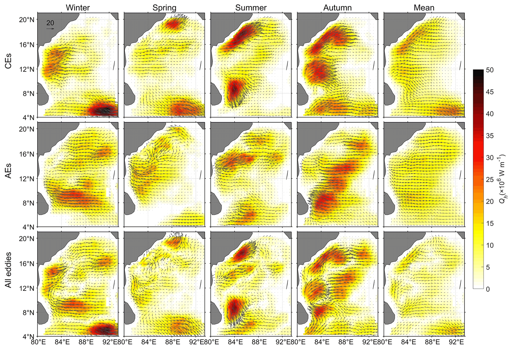
Figure 9Seasonal eddy-induced heat transport Qh in the Bay of Bengal: results for cyclonic eddies (CEs) (top row), results for anticyclonic eddies (AEs) (middle role), and results for all eddies (bottom row). Here, is a vector whose components are the meridional and zonal heat transports, the arrows indicate the transport direction, and the color indicates the transport magnitude.
Compared with θ′, the salinity anomalies S′ of eddies in the north and south bay present larger differences. Under the control of the low-salinity Bay of Bengal Water at the surface and the Indian Equatorial Water in the deep ocean (Stramma et al., 1996), the northern bay presents the salinity structures of positive S′ inside CEs and negative S′ inside AEs in the thermocline (upper panels in Fig. 7). The maximum S′ of CEs in spring can exceed +0.3 psu, whereas it is around +0.25 psu in autumn, and weakest in winter is only +0.2 psu. The extremum of negative S′ in AEs in autumn can reach −0.35 psu, values are around −0.25 psu in spring and summer, and −0.2 psu in winter. In addition, the S′ of CEs and AEs in the 30 dbar shallow surface water in summer and autumn exhibits some perturbation (positive/negative signals in CEs/AEs). For S′ in the southern bay (lower panels in Fig. 7), the magnitude of S′ signal is significantly small. Just in summer, the S′ of CEs and AEs exceed ±0.2 psu, while in other seasons, the S′ of CEs and AEs are less than 0.1 psu.
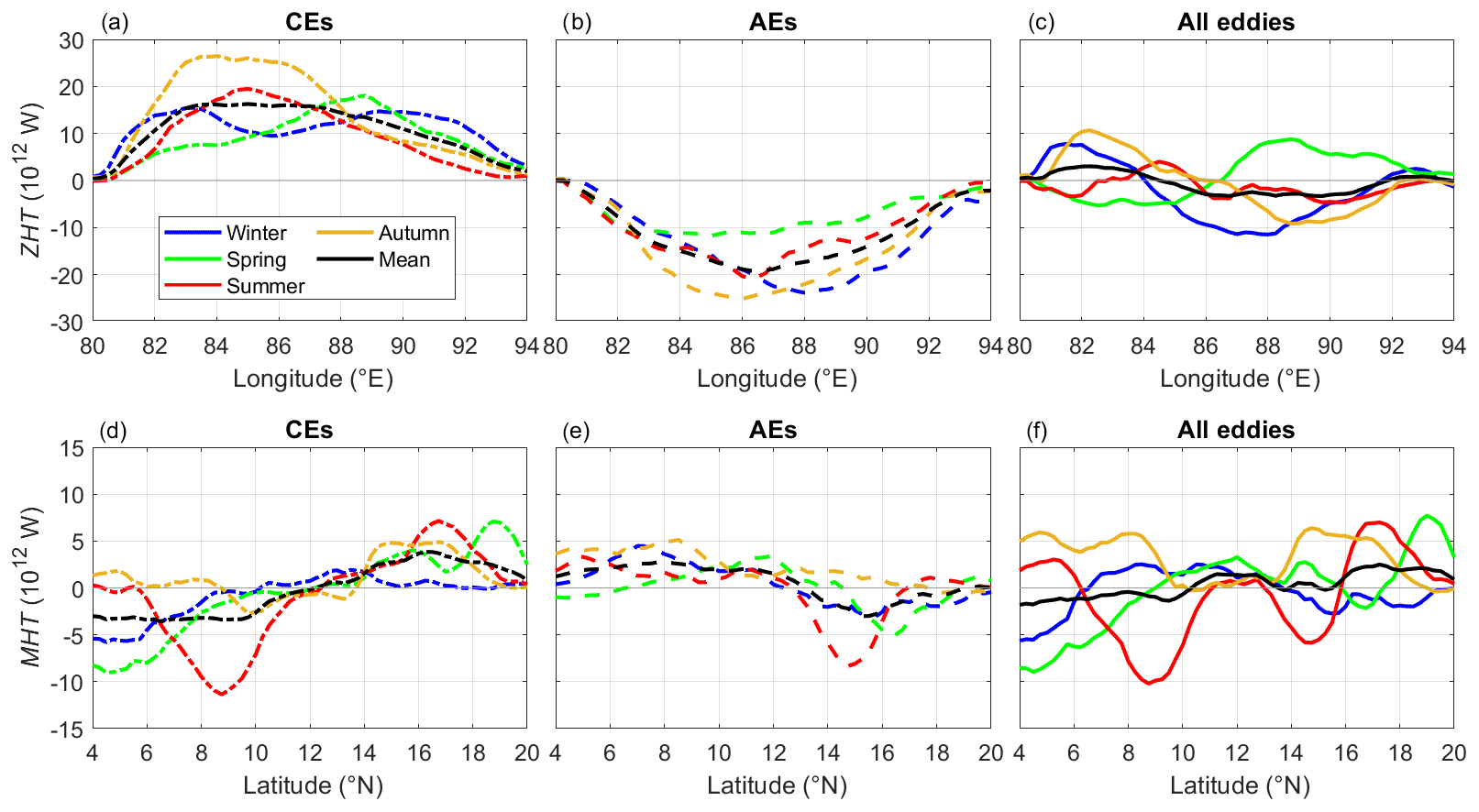
Figure 10The meridionally integrated zonal heat transport (ZHT, a–c) at different longitudes and the zonally integrated meridional heat transport (MHT, d–f) at different latitudes by cyclonic eddies (CEs), anticyclonic eddies (AEs), and all eddies in different seasons in the Bay of Bengal.
In addition, to verify the vertical thermohaline structure obtained from Argo profiles, the weekly ARMOR3D temperature and salinity field data were also used to analyze the seasonal variation in the vertical thermohaline structure of the eddies, and the corresponding results are drawn by dashed lines in Figs. 6 and 7. The seasonal variations in temperature and salinity signals are largely consistent with the result for the composite eddies based on the Argo profiles. Considering the full spatial coverage of the data, the spatial characteristics of the vertical thermohaline structure of the eddies in the Bay of Bengal was analyzed (Fig. 8). To ensure the accuracy of the data, we only calculated the average temperature and salt anomalies of subsurface water within the eddies (i.e., 50–150 dbar, which is the depth layer where eddies cause the greatest variations in temperature and salinity).
The spatial distribution of eddy-induced temperature anomalies is largely the same as the seasonal spatial distribution of eddies shown in Fig. 4; i.e., in areas where there are clustered eddies, the temperature anomaly is generally larger. The corresponding characteristic in spring is obvious; alternating CEs and AEs in the northwestern bay correspond to significant positive and negative variation in θ′, respectively. In summer and autumn, the clustered CEs in the northwestern bay and the Sri Lanka Dome cause large negative θ′, especially in the area to the east of Sri Lanka where the value of θ′ can exceed −3 ∘C. Similarly, AEs cause high positive values of θ′ in the western bay in summer and to the east of Sri Lanka in autumn. The spatial distribution of eddy-induced salinity anomalies is more complicated than that of temperature. In the region of the Bay of Bengal to the north of 12∘ N, the basic characteristics of CEs correspond to positive salinity anomalies, while those of AEs correspond to negative salinity anomalies. In the southern part to the south of 12∘ N, the salinity signal becomes turbulent owing to the invasion of the low-latitude equatorial circulation. For example, AEs present disordered positive salinity anomalies in the southern bay. Owing to differences in the salinity anomaly signal between the northern and southern parts of the bay, the perturbation of the salinity anomaly will appear in the surface during analysis of the 3D structure of one eddy in the entire Bay of Bengal (Fig. 7; Lin et al., 2019; Gulakaram et al., 2020). Some studies suggested that this reflects a salinity dipole structure in the near-surface layer due to the horizontal advection, eddy rotation, and background temperature/salinity meridional gradient (Melnichenko et al., 2017; Amores et al., 2017).
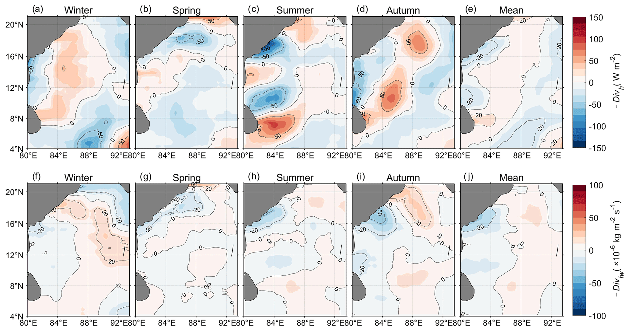
Figure 11Divergence of the heat transport (−Divh, a–e) and freshwater transport (−Divfw, f–j) caused by eddies in different seasons in the Bay of Bengal. Positive values represent oceanic heat/freshwater gains from eddies; negative values represent oceanic heat/freshwater losses by eddies.
Eddy heat transport is traditionally estimated within an Eulerian framework (Qiu and Chen, 2005; Roemmich and Gilson, 2001; Stammer, 1998), which does not explicitly identify eddy movements. In this study, similar to Dong et al. (2017), we considered changes in eddy structure along the paths of eddy propagation to estimate the eddy-induced heat and salt transport in the Bay of Bengal. Therefore, by combining the temperature and salinity anomalies of each eddy along the eddy path, provided by the weekly ARMOR3D temperature and salinity field data, with the details of eddy movement (propagation trajectory), provided by daily SLA fields, we estimated the eddy-induced heat and salt transport in different areas of the Bay of Bengal. The detailed method, as described in Sect. 2.2, considers not only the direction and speed of eddy propagation but also the variation in the properties of the intrinsic heat and salt during eddy movement.
4.1 Eddy-induced heat transport and its seasonal variation
The seasonal heat transport attributable to mesoscale eddies in the Bay of Bengal is illustrated in Fig. 9. It can be seen that CEs/AEs present eastward/westward heat transport in most regions due to CEs/AEs generally carrying negative/positive heat anomalies westward across the bay (upper and middle rows). The heat transport associated with CEs and AEs jointly determines the heat transport of all the eddies (bottom row). The eddy-induced heat transport is generally higher in regions where eddies are clustered. In the area to the south of 8∘ N, the southeast outside of the bay, the high eastward heat transport in winter and spring is related to the large-scale CEs that often appear there and move westward at a high speed (e.g., >10 cm s−1, Fig. 5). The seas to the east of Sri Lanka are dominated alternately by CEs and AEs in different seasons. Thus, in this region, the directions of heat transport are different in different seasons (e.g., in autumn and winter, westward-moving AEs lead to westward heat transport; in summer, northward-moving CEs lead to southward heat transport), and the magnitude of this transport is generally W m−1. The western bay is dominated by CEs and presents eastward heat transport in autumn and winter; conversely, it is dominated by AEs in spring and summer and presents westward heat transport. The eastern bay generally corresponds to westward heat transport in autumn and winter, due to the prevalence of AEs moving westward in the seasons (Cheng et al., 2018).
We integrated the zonal heat transport Qhz by mesoscale eddies at each 0.25∘ grid from north to south and obtained the integrated zonal heat transport ZHT = ∫Qhzdy in the entire meridional direction, where dy is the meridional unit distance (unit: m) such that the unit of ZHT is watt (abbreviated W). Similarly, the zonally integrated meridional heat transport MHT can be expressed as MHT = ∫Qhmdx, where Qhm is the meridional heat transport and dx is the zonal unit distance. The seasonal eddy-induced ZHT at different longitudes and MHT at different latitudes in the whole Bay of Bengal are shown in Fig. 10. In terms of ZHT, CEs/AEs present overall eastward/westward (positive/negative) heat transport in all seasons (Fig. 10a and b), and the maximum transport efficiency can be of the order of 10–20×1012 W at the longitudes of 84–88∘ E, corresponding to the eddy-rich regions in the northwestern bay (Fig. 4). Comparison with ZHT, eddy-induced MHT is substantially smaller (Fig. 10d–f). The magnitude of the seasonal MHT of CEs and AEs is almost below 5×10¹² W. CEs and AEs show almost opposite phase changes in the direction of MHT. In the northern bay to the north of 12∘ N, where most eddies move southward (Fig. 5), the CEs and AEs exhibit northward (positive) and southward (negative) heat transport, respectively. Conversely, in the southern bay to the south of 12∘ N, where eddies tend to move northward, the CEs and AEs exhibit southward and northward heat transport, respectively. Owing to the seasonal variation in eddies in the Bay of Bengal, the ZHT and MHT of all eddies vary substantially in different seasons (Fig. 10c and f).
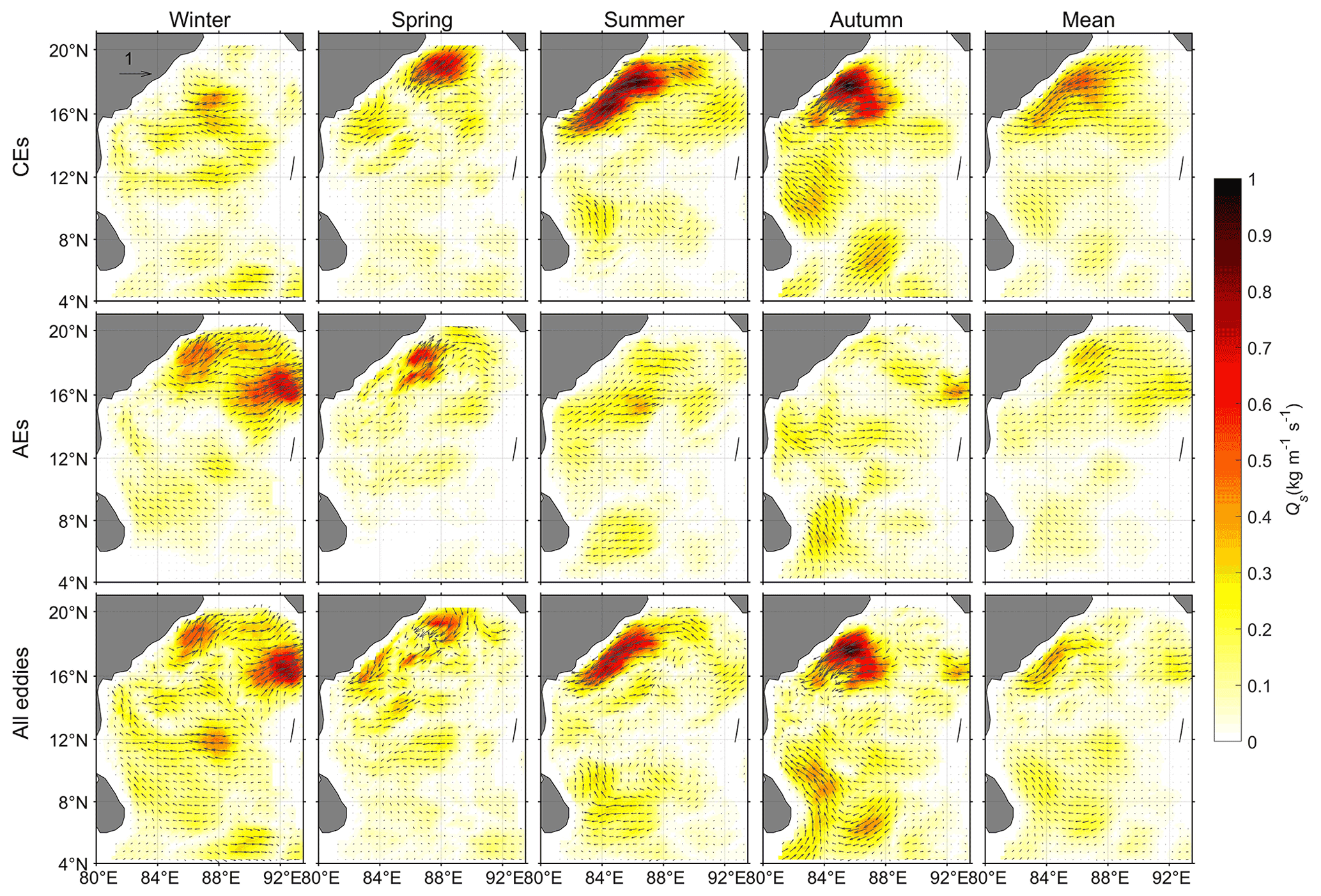
Figure 12Seasonal eddy-induced salt transport Qs in the Bay of Bengal: results for cyclonic eddies (CEs) (upper row), results for anticyclonic eddies (AEs) (middle row), and results for all eddies (bottom row). Here, is a vector whose components are the meridional and zonal salt transports, the arrows indicate the transport direction, and the color indicates the transport magnitude.
To estimate the impact of heat transports by eddy movements in the Bay of Bengal, we calculated the divergence of eddy heat transports Divh and smoothed it using a moving average filter with a half-width of 5∘ longitude and 3∘ latitude. The divergence of the heat transports Divh is calculated as Div; here Qh=(QhzQhm) is the horizontal heat transport vector and ∇⋅ is the horizontal divergence operator. Divh represents the heat flux by eddy movements in the horizontal direction; the unit is W m−2. Figure 11a–e show −Divh in different seasons in the Bay of Bengal. Positive values of −Divh represent oceanic heat gains from eddies, and negative values represent oceanic heat losses, which means heat is transported away by eddies.
In terms of the annual mean result (Fig. 11e), the ocean loses heat due to eddy movements in the eastern, southeastern, and western coastal regions of the bay, while the ocean gains heat from eddies in the northern and central regions. The magnitude of the ocean heat loss/gain caused by eddy movements is about 10–20 W m−2, of which the heat loss can reach 20 W m−2 in the southern and western coastal areas of the bay. As a comparison, the annual mean air–sea net heat flux at the surface in the Bay of Bengal is on the order of 20–50 W m−2 (Sanchez-Franks et al., 2018; Pokhrel et al., 2020; also see Fig. S4). The eddy-induced heat flux is comparable in magnitude with the air–sea net heat flux, implying that the mesoscale eddies can exert a strong impact on the oceanic heat transport and redistribution in the Bay of Bengal. In addition, −Divh caused by eddies varies substantially in different seasons. In autumn and winter, the geographical distribution of −Divh is similar to the annual mean result, showing a sandwich structure of ocean heat-loss–gain–loss from west to east. In spring, ocean heat loss is seen overall, with ocean heat gain only in limited areas in the western and northeastern parts. In summer, due to the strong eddy activities, the heat gain and heat loss alternately appear in the western part of the bay from north to south, and the magnitude can exceed 50 W m−2. Despite air–sea net heat flux into the ocean in the eastern seas of Sri Lanka, a cold pool is still formed there in summer due to the intrusion of cold water carried by the Southwest Monsoon Current (SMC, Vinayachandran et al., 2020; Das et al., 2016). The high eddy-induced ocean heat gain here suggests that eddy activities (mainly the northward input of AEs carrying warm waters and the northward outflow of CEs carrying cold waters) would somewhat balance the heat loss due to the SMC intrusion. Without the heat input from eddy movements, the temperature of the summer cold pool caused by SMC intrusion would be lower, and the lower summer cold pool might change the direction of the air–sea heat flux. Compared with the large-scale air–sea heat flux, the eddy-induced heat transport can contribute substantially to regional and basin-scale heat variability.
4.2 Eddy-induced salt transport and its seasonal variation
The spatial distribution of eddy-induced salt transport Qs in the Bay of Bengal is shown in Fig. 12. In the part of the bay to the north of 12∘ N, the salinity anomalies caused by eddies are relatively uniform with little interference by surface disturbances, and the salt transport Qs is basically westward/eastward for CEs/AEs (CEs/AEs carry positive/negative salinity anomalies moving westward – westward/eastward salt transport). The high salt transport of all eddies is also concentrated in the northern part. In winter, AEs dominate the salt transport eastward and northeastward; in spring, summer, and autumn, CEs dominate southwestward salt transport, which causes the salinity to decrease in the northern bay. The Qs in the part of the bay to the south of 12∘ N is notably smaller than that in the northern part. The reason for the low salt transport in the southern part is related not only to the small number of eddies and their weak strength but also to the complex structure of salinity anomalies caused by the eddies. In Sect. 3.2, the spatial characteristics of the vertical salinity anomalies of eddies (Fig. 8) shows that the salinity signals in the southern bay become turbulent, which may be caused by the invasion of the low-latitude equatorial circulation (Cui et al., 2021). Disturbance of salinity anomaly signals in the surface or subsurface waters reduces the salt transport capacity of CEs and AEs over the entire vertical structure.
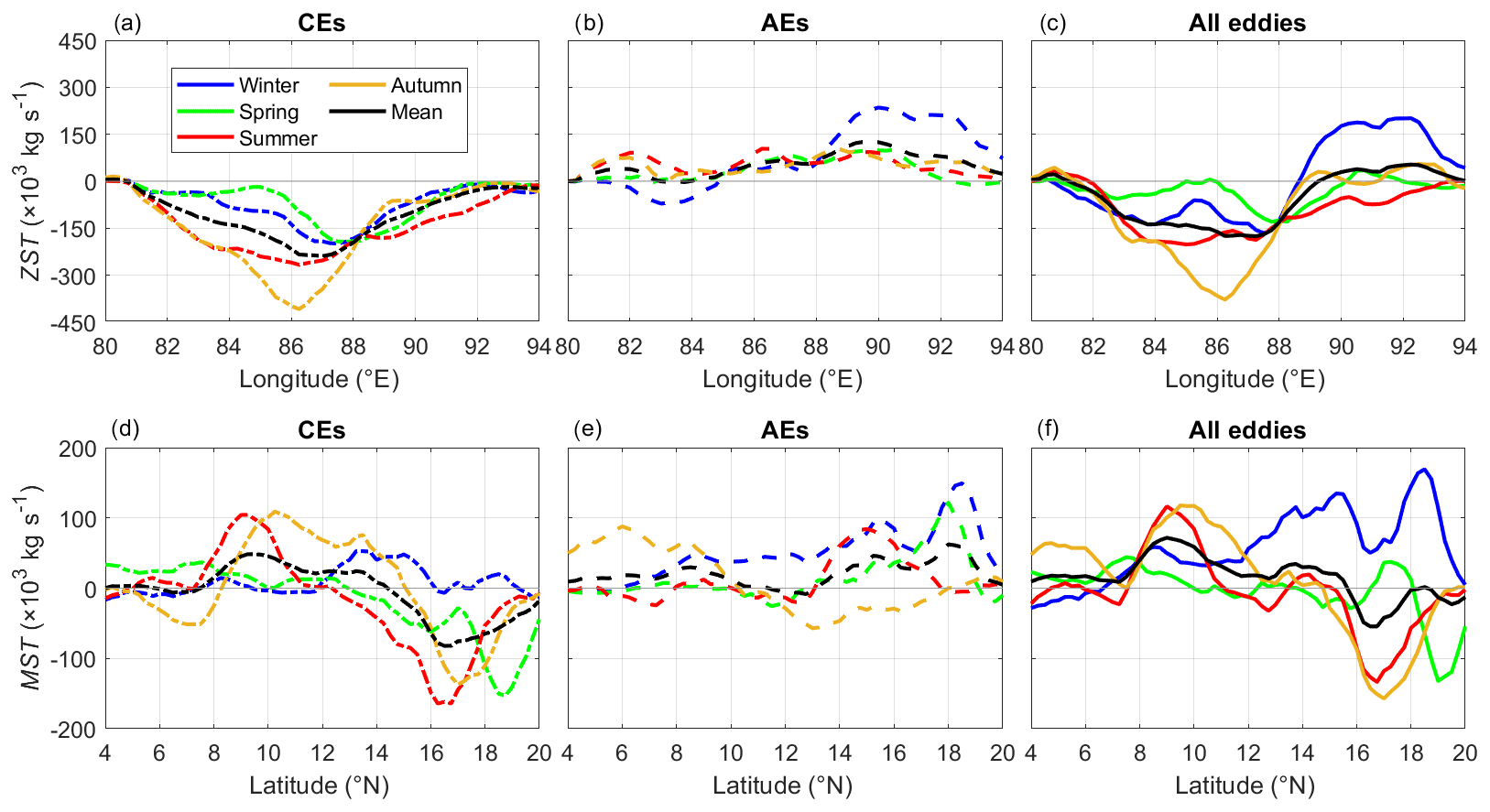
Figure 13The meridionally integrated zonal salt transport (ZST, a–c) at different longitudes and the zonally integrated meridional salt transport (MST, d–f) at different latitudes by cyclonic eddies (CEs), anticyclonic eddies (AEs), and all eddies in different seasons in the Bay of Bengal.
Figure 13 shows the meridionally integrated zonal salt transport ZST = ∫Qszdy and the zonally integrated meridional salt transport MST = ∫Qsmdx caused by eddies, which represent the salt flux (unit: kg s−1) in the entire meridional and zonal directions, respectively. The ZST direction of all eddies is largely consistent with that of CEs. The maximum ZST of CEs in autumn is greater than 400×103 kg s−1 at the longitude of about 86∘ N. The ZST of AEs is relatively low, except in winter, the magnitude in other seasons is less than 100×103 kg s−1. In terms of MST, the magnitude of the mean transport is kg s−1 for both CEs and AEs, which is substantially smaller than that of ZST (black lines in Fig. 13). The MST direction of CEs is southward in the northern bay and northward in the southern bay. Northward salt transport of AEs is presented almost in the entire bay. The combined effect of CEs and AEs results in southward MST in the area to the north of 16∘ N and northward MST in the central and southern parts (Fig. 13f).
To estimate the impact of salt transports by eddy movements in the Bay of Bengal, we calculated the divergence of eddy salt transports Div and smoothed it using a moving average filter with a half-width of 5∘ longitude and 3∘ latitude. Salt transport can be treated as an equivalent freshwater transport assuming conservation of mass across the transport section (Div), where mean upper-ocean salinity is s0=35 psu. Divfw represents the equivalent freshwater flux by eddy movements in the horizontal direction; the unit is kg m−2 s−1. Figure 11f–j show −Divfw in different seasons in the Bay of Bengal, positive values of −Divfw represent oceanic freshwater gains from eddies, and negative values represent oceanic freshwater losses by eddies. In terms of the annual mean result (Fig. 11j), the ocean gains and loses freshwater due to eddy movements in the east and west of the bay, respectively. The magnitude of the freshwater loss/gain is generally 0– kg m−2 s−1, of which the freshwater loss in the western coastal areas of the bay exceeds kg m−2 s−1. Compared with the north–south variation in the annual mean net freshwater flux at the surface (Fig. S4), the spatial distribution of −Divfw shows an east–west variation, which indicates that mesoscale eddies play an important role in maintaining the east–west freshwater or salt balance in the Bay of Bengal. Owing to the seasonal variation in eddy activities in the Bay of Bengal, the −Divfw caused by eddies varies substantially. The northernmost part of the bay exhibits freshwater losses only in winter and freshwater gains in the rest of the seasons, and the maximum freshwater gain in autumn can exceed kg m−2 s−1. The EICC area in the western bay shows eddy-induced freshwater losses in spring, summer, and autumn, and the extreme value in autumn can reach kg m−2 s−1. The eastern part of the bay presents freshwater gains of greater than kg m−2 s−1 in winter. The magnitude of freshwater gains and losses in the southern part of the bay is small in all seasons, which is mainly related to the weaker salt transport caused by the inconsistency of the salinity signal within eddies (Fig. 8).
The Bay of Bengal, occupying the eastern part of the tropical Indian Ocean, is characterized by the seasonal circulation and intense eddy activity throughout the year. The mesoscale eddies in the Bay of Bengal were determined from satellite altimetry data spanning over 26 years from January 1993 to February 2019. The eddy result revealed that mesoscale eddy activity in the Bay of Bengal has evident seasonal variation.
Generally, there are three main areas of distribution of mesoscale eddies in the Bay of Bengal. One is the EICC region in the west and northwest of the bay, indicating that variation or reversal of the western boundary current EICC will often shed rich eddy structures, especially in spring and summer. Another region is the northeastern part and the eastern boundary, where eddies generated in spring and summer move southwestward into the central bay in autumn (some even reach the western bay). The eddies are mainly driven by equatorial zonal winds, with both nonlinearity and coastline geometry essential for eddy generation (Cheng et al., 2018). The third region is seas to the east of Sri Lanka, where there are strong CEs (Sri Lanka Dome) in summer and AEs in autumn. The Sri Lanka Dome develops during the Southwest Monsoon, in response to the strong cyclonic curl in the local wind field and the northeastward Southwest Monsoon Current invading the bay (Murty et al., 1992; Burns et al., 2017; Cullen et al., 2022). In addition, the eddy propagation speed in different seasons also shows some differences. The westward speed of eddies is fastest in winter and slowest in summer. Moreover, eddy propagation directions were clearly bounded by the 12∘ N line of latitude; eddies to the north/south move westward and slightly southward/northward. The different directions and speeds of propagation of eddies in different seasons are crucial to estimation of the magnitude of the seasonal transport of eddies in the Bay of Bengal.
Based on satellite altimetry data in combination with Argo profile or 3D reprocessed thermohaline fields, the eddy synthesis method was used to construct vertical temperature and salinity structures of eddies in the Bay of Bengal. The vertical thermohaline structure of eddies in the Bay of Bengal shows obvious seasonal variation as well as some differences for the northern and southern subregions. The θ′ values of CEs and AEs are both at a maximum in spring (up to ±2.5 ∘C) and at a minimum in winter (about ±1.2 ∘C) for the northern bay. The minimum θ′ in winter is not only related to the smaller eddy amplitude (Fig. 4a and e) but also to the thicker barrier layer in this season (Thadathil et al., 2007), which attenuates temperature changes through vertical movement of the waterbody. The maximum θ′ of CEs in the southern bay in summer is associated with the persistent and strong Sri Lanka Dome which often appears in May and disappears in September. CEs (AEs) produce notable positive (negative) S′ signals at the subsurface in the northern bay but with a small magnitude in the southern bay. The spatial distribution of eddy-induced salinity anomalies illustrates that the salinity signal becomes turbulent owing to the invasion of the low-latitude equatorial circulation. For example, AEs present disordered positive salinity anomalies in the southern bay. Owing to differences in the salinity anomaly signal between the northern and southern parts of the bay, the perturbation of the salinity anomaly will appear in the surface during analysis of the 3D structure of one eddy in the entire Bay of Bengal (Fig. 7; Lin et al., 2019; Gulakaram et al., 2020). Some studies suggested that this reflects a salinity dipole structure in the near-surface layer due to the horizontal advection, eddy rotation, and background temperature/salinity meridional gradient (Melnichenko et al., 2017; Amores et al., 2017). If the average thermohaline structure of the entire region were used to estimate the eddy-induced heat/salt transport, the marked regional characteristics would be smoothed.
By combining the temperature and salinity anomalies of eddies, provided by the weekly ARMOR3D thermohaline field data, with the details of eddy movement (propagation trajectory), provided by gridded multimission altimeter products, we estimated the eddy-induced heat and salt transport in different areas of the Bay of Bengal. Generally, high heat and salt transport is concentrated in eddy-rich regions, e.g., the western, northwestern and eastern parts of the bay, the seas to the east of Sri Lanka, and the region to the southeast outside of the bay. The southern part of the bay shows weak salt transport owing to the inconsistent salinity signal within eddies. Owing to obvious seasonal variation in eddy activities, the heat and salt transport in different seasons also changes substantially. The magnitude of the seasonal ZHT of CEs and AEs in the whole bay is in the order of 10×1012 W, with higher values in autumn and winter and smaller values in spring and summer. The result is basically the same with theoretical calculation by Gonaduwage et al. (2019) in the distribution of high eddy transport, but there are some differences in the direction and magnitude of eddy transport. Gonaduwage et al. (2019) adopted the eddy diffusivity method for eddy transport estimation based on integral timescales of sea surface variability and near-surface eddy kinetic energy. The details of eddy movements and eddy-induced temperature and salinity anomalies in different regions were not considered in their analysis. The findings based on measured temperature and salt data show that diverse seasonal changes in temperature and salinity in the Bay of Bengal might cause substantial deviation in eddy-induced heat/salt transport estimated theoretically.
To estimate the impact of heat/salt transports by eddy movements in the Bay of Bengal, the divergence of eddy heat/freshwater transports was calculated. The 10–20 W m−2 value of the eddy-induced heat flux is comparable in magnitude with the annual mean air–sea net heat flux, implying that the mesoscale eddies can exert a strong impact on the oceanic heat transport and redistribution in the Bay of Bengal. Notably, the high eddy-induced ocean heat gain in the eastern seas of Sri Lanka in summer suggests that eddy activities would somewhat balance the heat loss due to the intrusion of cold water carried by the Southwest Monsoon Current. Without the heat input from eddy movements, the temperature of the summer cold pool caused by SMC intrusion would be lower, and the lower summer cold pool might change the direction of the air–sea heat flux. Compared with the north–south variation in the annual mean net freshwater flux at the surface, the spatial distribution of eddy-induced freshwater flux (the magnitude is generally 0– kg m−2 s−1; seasonal variation is higher: up to kg m−2 s−1 regionally) shows an east–west variation, which indicates that mesoscale eddies play an important role in maintaining the east–west freshwater or salt balance in the Bay of Bengal. Compared with the large-scale air–sea heat flux and net freshwater flux at the surface, the eddy-induced heat/freshwater transport can contribute substantially to regional and basin-scale heat/freshwater variability. This work provides data that could support further research on the heat and salt balance of the entire Bay of Bengal.
The altimeter products (SEALEVEL_GLO_PHY_L4_REP_OBSERVATION_008_47) and the Global ARMOR3D L4 reprocessed dataset (MULTIOBS_GLO_PHY_REP_015_002) used here are distributed by the European Copernicus Marine Environment Monitoring Service (CMEMS, http://marine.copernicus.eu, last access on 12 August 2021, CMEMS, 2021a, b). The Argo profiles are provided by Coriolis Global Data Acquisition Center (http://www.coriolis.eu.org, last access: 3 May 2022, Coriolis, 2022).
The supplement related to this article is available online at: https://doi.org/10.5194/os-18-1645-2022-supplement.
JY and JZ designed the experiments and WC carried them out. WC performed the data analyses and drafted the paper. WC prepared the paper with contributions from all co-authors.
The contact author has declared that none of the authors has any competing interests.
Publisher’s note: Copernicus Publications remains neutral with regard to jurisdictional claims in published maps and institutional affiliations.
We thank two anonymous reviewers for helpful comments on an earlier version of this paper. We acknowledge all the data providers for the data utilized in this study.
This research has been supported by the National Natural Science Foundation of China (grant no. 42106178), the Basic Scientific Fund for National Public Research Institutes of China (grant no. 2020Q07), the Science Foundation of Donghai Laboratory (grant no. DH-2022KF01014), and the Shandong Provincial Natural Science Foundation (grant no. ZR2021QD006).
This paper was edited by Karen J. Heywood and reviewed by two anonymous referees.
Akhil, V. P., Durand, F., Lengaigne, M., Vialard, J., Keerthi, M. G., Gopalakrishna, V. V., and de Boyer Montégut, C.: A modeling study of the processes of surface salinity seasonal cycle in the Bay of Bengal, J. Geophys. Res.-Oceans, 119, 3926–3947, 2014.
Amores, A., Melnichenko, O., and Maximenko, N.: Coherent mesoscale eddies in the North Atlantic subtropical gyre: 3-D structure and transport with application to the salinity maximum, J. Geophys. Res.-Oceans, 122, 23–41, 2017.
Babu, M. T., Kumar, P. S., and Rao, D. P.: A subsurface cyclonic eddy in the Bay of Bengal, J. Mar. Res., 49, 403–410, 1991.
Babu, M. T., Sarma, Y. V. B., Murty, V. S. N., and Vethamony, P.: On the circulation in the Bay of Bengal during northern spring inter-monsoon (March–April 1987), Deep Sea Res. Pt. II, 50, 855–865, 2003.
Burns, J. M., Subrahmanyam, B., and Murty, V. S. N.: On the dynamics of the Sri Lanka Dome in the Bay of Bengal, J. Geophys. Res.-Oceans, 122, 7737–7750, 2017.
Chaigneau, A., Eldin, G., and Dewitte, B.: Eddy activity in the four major upwelling systems from satellite altimetry (1992–2007), Prog. Oceanogr., 83, 117–123, 2009.
Chaigneau, A., Gizolme, A., and Grados, C.: Mesoscale eddies off Peru in altimeter records: Identification algorithms and eddy spatio-temporal patterns, Prog. Oceanogr., 79, 106–119, 2008.
Chaigneau, A., Le Texier, M., Eldin, G., Grados, C., and Pizarro, O.: Vertical structure of mesoscale eddies in the eastern South Pacific Ocean: A composite analysis from altimetry and Argo profiling floats, J. Geophys. Res.-Oceans, 116, C11025, https://doi.org/10.1029/2011JC007134, 2011.
Chelton, D. B., Gaube, P., Schlax, M. G., Early, J. J., and Samelson, R. M.: The influence of nonlinear mesoscale eddies on near-surface oceanic chlorophyll, Science, 334=, 328–332, 2011b.
Chelton, D. B., Schlax, M. G., and Samelson, R. M.: Global observations of nonlinear mesoscale eddies, Prog. Oceanogr., 91, 167–216, 2011a.
Chen, G., Han, W., Li, Y., McPhaden, M. J., Chen, J., Wang, W., and Wang, D.: Strong intraseasonal variability of meridional currents near 5 N in the Eastern Indian Ocean: Characteristics and causes, J. Phys. Oceanogr., 47, 979–998, 2017.
Chen, G., Li, Y., Xie, Q., and Wang, D.: Origins of eddy kinetic energy in the Bay of Bengal, J. Geophys. Res.-Oceans, 123, 2097–2115, 2018.
Chen, G., Wang, D., and Hou, Y.: The features and interannual variability mechanism of mesoscale eddies in the Bay of Bengal, Cont. Shelf Res., 47, 178–185, 2012.
Cheng, X., McCreary, J. P., Qiu, B., Qi, Y., Du, Y., and Chen, X.: Dynamics of eddy generation in the central Bay of Bengal, J. Geophys. Res.-Oceans, 123, 6861–6875, 2018.
Cheng, X., Xie, S. P., McCreary, J. P., Qi, Y., and Du, Y.: Intraseasonal variability of sea surface height in the Bay of Bengal, J. Geophys. Res.-Oceans, 118, 816–830, 2013.
CMEMS: Global Ocean Gridded L4 Sea Surface Heights And Derived Variables Reprocessed (SEALEVEL_GLO_PHY_L4_REP_OBSERVATION_008_47), http://marine.copernicus.eu, [data set], last access on 12 August 2021.
CMEMS: Multi Observation Global Ocean 3D Temperature Salinity Height Geostrophic Current and MLD (MULTIOBS_GLO_PHY_REP_015_002), http://marine.copernicus.eu, [data set], last access on 12 August 2021.
Coriolis: The Argo profiles are provided by Coriolis Global Data Acquisition Center, http://www.coriolis.eu.org, [data set], last access: 3 May 2022.
Cui, W., Yang, J., and Ma, Y.: A statistical analysis of mesoscale eddies in the Bay of Bengal from 22–year altimetry data, Acta Ocean. Sin., 35, 16–27, 2016.
Cui, W., Zhou, C., Zhang, J., and Yang, J.: Statistical characteristics and thermohaline properties of mesoscale eddies in the Bay of Bengal, Acta Ocean. Sin., 40, 10–22, 2021.
Cullen, K., Shroyer, E., and O'Neill, L.: Weakly Nonlinear Ekman Pumping in the Sri Lanka Dome and Southwest Monsoon Current, J. Phys. Ocean., 52, 1693–1703, 2022.
Dandapat, S. and Chakraborty, A.: Mesoscale eddies in the Western Bay of Bengal as observed from satellite altimetry in 1993–2014: statistical characteristics, variability and three-dimensional properties, IEEE J. Sel. Top. Appl., 9, 5044–5054, 2016.
Das, U., Vinayachandran, P. N., and Behara, A.: Formation of the southern Bay of Bengal cold pool, Clim. Dynam., 47, 2009–2023, 2016.
Dong, C., McWilliams, J. C., Liu, Y., and Chen, D.: Global heat and salt transports by eddy movement, Nat. Commun., 5, 1–6, 2014.
Dong, D., Brandt, P., Chang, P., Schütte, F., Yang, X., Yan, J., and Zeng, J.: Mesoscale eddies in the northwestern Pacific Ocean: Three-dimensional eddy structures and heat/salt transports, J. Geophys. Res.-Oceans, 122, 9795–9813, 2017.
Eigenheer, A. and Quadfasel, D.: Seasonal variability of the Bay of Bengal circulation inferred from TOPEX/Poseidon altimetry, J. Geophys. Res.-Oceans, 105, 3243–3252, 2000.
Fu, L. L.: Pattern and velocity of propagation of the global ocean eddy variability, J. Geophys. Res.-Oceans, 114, C11017. https://doi.org/10.1029/2009JC005349, 2009.
Gonaduwage, L. P., Chen, G., McPhaden, M. J., Priyadarshana, T., Huang, K., and Wang, D.: Meridional and zonal eddy-induced heat and salt transport in the Bay of Bengal and their seasonal modulation, J. Geophys. Res.-Oceans, 124, 8079–8101, 2019.
Graham, N. E. and Barnett, T. P.: Sea surface temperature, surface wind divergence, and convection over tropical oceans, Science, 238, 657–659, 1987.
Guinehut, S., Dhomps, A.-L., Larnicol, G., and Le Traon, P.-Y.: High resolution 3-D temperature and salinity fields derived from in situ and satellite observations, Ocean Sci., 8, 845–857, https://doi.org/10.5194/os-8-845-2012, 2012.
Gulakaram, V. S., Vissa, N. K., and Bhaskaran, P. K.: Characteristics and vertical structure of oceanic mesoscale eddies in the Bay of Bengal, Dynam. Atmos. Oceans, 89, 101131, https://doi.org/10.1016/j.dynatmoce.2020.101131, 2020.
Hacker, P., Firing, E., Hummon, J., Gordon, A. L., and Kindle, J. C.: Bay of Bengal currents during the northeast monsoon, Geophys. Res. Lett., 25, 2769–2772, 1998.
Henson, S. A. and Thomas, A. C.: A census of oceanic anticyclonic eddies in the Gulf of Alaska, Deep Sea Res. Pt. I, 55, 163–176, 2008.
Kumar, B. and Chakraborty, A.: Movement of seasonal eddies and its relation with cyclonic heat potential and cyclogenesis points in the Bay of Bengal, Nat. Hazards, 59, 1671, https://doi.org/10.1007/s11069-011-9858-9, 2011.
Kumari, A., Kumar, S. P., and Chakraborty, A.: Seasonal and interannual variability in the barrier layer of the Bay of Bengal, J. Geophys. Res.-Oceans, 123, 1001–1015. https://doi.org/10.1002/2017JC013213, 2018.
Le Traon, P. Y. and Dibarboure, G.: An illustration of the contribution of the TOPEX/Poseidon – Jason-1 tandem mission to mesoscale variability studies, Mar. Geodesy, 27, 3–13, 2004.
Lin, X., Qiu, Y. and Sun, D.: Thermohaline Structures and Heat/Freshwater Transports of Mesoscale Eddies in the Bay of Bengal Observed by Argo and Satellite Data, Remote Sens., 11, 2989, https://doi.org/10.3390/rs11242989, 2019.
Luo, H., Bracco, A., and Di Lorenzo, E.: The interannual variability of the surface eddy kinetic energy in the Labrador Sea, Prog. Oceanogr., 91, 295–311, 2011.
Melnichenko, O., Amores, A., Maximenko, N., Hacker, P., and Potemra, J.: Signature of mesoscale eddies in satellite sea surface salinity data, J. Geophys. Res.-Oceans, 122, 1416–1424, 2017.
Murty, V. S. N., Sarma, Y. V. B., Rao, D. P., and Murty, C. S.: Water characteristics, mixing and circulation in the Bay of Bengal during southwest monsoon, J. Mar. Res., 50, 207–228, 1992.
Murty, V. S. N., Subrahmanyam, B., Gangadhara Rao, L. V., and Reddy, G. V.: Seasonal variation of sea surface temperature in the Bay of Bengal during 1992 as derived from NOAA-AVHRR SST data, Int. J. Remote Sens., 19, 2361–2372, 1998.
Nencioli, F., Dong, C., Dickey, T., Washburn, L., and McWilliams, J. C.: A vector geometry–based eddy detection algorithm and its application to a high-resolution numerical model product and high-frequency radar surface velocities in the Southern California Bight, J. Atmos. Ocean. Tech., 27, 564–579, 2010.
Nuncio, M. and Kumar, S. P.: Life cycle of eddies along the western boundary of the Bay of Bengal and their implications, J. Mar. Syst., 94, 9–17, 2012.
Patnaik, K. V. K. R. K., Maneesha, K., Sadhuram, Y., Prasad, K. V. S. R., Ramana Murty, T. V., and Brahmananda Rao, V.: East India Coastal Current induced eddies and their interaction with tropical storms over Bay of Bengal, J. Operat. Ocean., 7, 58–68, 2014.
Pokhrel, S., Dutta, U., Rahaman, H., Chaudhari, H., Hazra, A., Saha, S. K., and Veeranjaneyulu, C.: Evaluation of different heat flux products over the tropical Indian Ocean, Earth Space Sci., 7, e2019EA000988, https://doi.org/10.1029/2019EA000988, 2020.
Prasad, T. G.: Annual and seasonal mean buoyancy fluxes for the tropical Indian Ocean, Current Sci., 73, 667–674, 1997.
Prasanna Kumar, S., Nuncio, M., Narvekar, J., Kumar, A., Sardesai, D. S., De Souza, S. N., and Madhupratap, M.: Are eddies nature's trigger to enhance biological productivity in the Bay of Bengal, Geophys. Res. Lett., 31, L07309, https://doi.org/10.1029/2003GL019274, 2004.
Qiu, B. and Chen, S.: Eddy-induced heat transport in the subtropical North Pacific from Argo, TMI, and altimetry measurements, J. Phys. Ocean., 35, 458–473, 2005.
Qiu, Y., Li, L., Yu, W., and Hu, J.: Annual and interannual variations of sea-level anomaly in the Bay of Bengal and the Andaman Sea, Acta Ocean. Sin., 26, 13–29, 2007.
Rao, R. R. and Sivakumar, R.: Seasonal variability of sea surface salinity and salt budget of the mixed layer of the north Indian Ocean, J. Geophys. Res.-Oceans, 108, 3009, https://doi.org/10.1029/2001JC000907, 2003.
Rao, S. A., Gopalakrishna, V. V., Shetye, S. R., and Yamagata, T.: Why were cool SST anomalies absent in the Bay of Bengal during the 1997 Indian Ocean Dipole Event, Geophys. Res. Lett., 29, 1555, https://doi.org/10.1029/2001GL014645, 2002.
Robinson, I. S.: Mesoscale ocean features: Eddies, In Discovering the Ocean from Space, Springer, Berlin, Heidelberg, 69–114, 2010.
Roemmich, D. and Gilson, J.: Eddy transport of heat and thermocline waters in the North Pacific: A key to interannual/decadal climate variability, J. Phys. Ocean., 31, 675–687, 2001.
Sanchez-Franks, A., Kent, E. C., Matthews, A. J., Webber, B. G., Peatman, S. C., and Vinayachandran, P. N.: Intraseasonal variability of air–sea fluxes over the Bay of Bengal during the southwest monsoon, J. Climate, 31, 7087–7109, 2018.
Seo, H., Subramanian, A. C., Song, H., and Chowdary, J. S.: Coupled effects of ocean current on wind stress in the Bay of Bengal: Eddy energetics and upper ocean stratification, Deep Sea Res. Pt. II, 168, 104617, https://doi.org/10.1016/j.dsr2.2019.07.005, 2019.
Shenoi, S. S. C., Shankar, D., and Shetye, S. R.: Differences in heat budgets of the near-surface Arabian Sea and Bay of Bengal: Implications for the summer monsoon, J. Geophys. Res.-Oceans, 107, 3052, https://doi.org/10.1029/2000JC000679, 2002.
Somayajulu, Y. K., Murty, V. S. N., and Sarma, Y. V. B.: Seasonal and inter-annual variability of surface circulation in the Bay of Bengal from TOPEX/Poseidon altimetry, Deep Sea Res. Pt. II, 50, 867–880, 2003.
Souza, J. M. A. C., de Boyer Montégut, C., and Le Traon, P. Y.: Comparison between three implementations of automatic identification algorithms for the quantification and characterization of mesoscale eddies in the South Atlantic Ocean, Ocean Sci., 7, 317–334, https://doi.org/10.5194/os-7-317-2011, 2011.
Sreenivas, P., Gnanaseelan, C., and Prasad, K. V. S. R.: Influence of El Niño and Indian Ocean Dipole on sea level variability in the Bay of Bengal, Global Planet. Change, 80, 215–225, 2012.
Stammer, D.: On eddy characteristics, eddy transports, and mean flow properties, J. Phys. Ocean., 28, 727–739, 1998.
Stramma, L., Fischer, J., and Schott, F.: The flow field off southwest India at 8∘ N during the southwest monsoon of August 1993, J. Mar. Res., 54, 55–72, 1996.
Thadathil, P., Muraleedharan, P. M., Rao, R. R., Somayajulu, Y. K., Reddy, G. V., and Revichandran, C.: Observed seasonal variability of barrier layer in the Bay of Bengal, J. Geophys. Res.-Oceans, 112, C02009, https://doi.org/10.1029/2006JC003651, 2007.
Varkey, M. J., Murty, V. S. N., and Suryanarayana, A.: Physical oceanography of the Bay of Bengal and Andaman Sea, Ocean. Mar. Biol., 34, 1–70, 1996.
Vinayachandran, P. N. and Yamagata, T.: Monsoon Response of the Sea around Sri Lanka: Generation of Thermal Domesand Anticyclonic Vortices, J. Phys. Ocean., 28, 1946–1960, 1998.
Vinayachandran, P. N., Masumoto, Y., Mikawa, T., and Yamagata, T.: Intrusion of the southwest monsoon current into the Bay of Bengal, J. Geophys. Res.-Oceans, 104, 11077–11085, 1999.
Vinayachandran, P. N., Murty, V. S. N., and Ramesh Babu, V.: Observations of barrier layer formation in the Bay of Bengal during summer monsoon, J. Geophys. Res.-Oceans, 107, 8018, https://doi.org/10.1029/2001JC000831, 2002.
Vinayachandran, P. N., Das, U., Shankar, D., Jahfer, S., Behara, A., Nair, T. B., and Bhat, G. S.: Maintenance of the southern Bay of Bengal cold pool, Deep Sea Res. Pt. II, 179, 104624, https://doi.org/10.1016/j.dsr2.2019.07.012, 2020.
Xu, C., Shang, X. D., and Huang, R. X.: Estimate of eddy energy generation/dissipation rate in the world ocean from altimetry data, Ocean Dynam., 61, 525–541, 2011.
Yang, G., Wang, F., Li, Y., and Lin, P.: Mesoscale eddies in the northwestern subtropical Pacific Ocean: Statistical characteristics and three-dimensional structures, J. Geophys. Res.-Oceans, 118, 1906–1925, 2013.
Zhang, Z., Wang, W., and Qiu, B.: Oceanic mass transport by mesoscale eddies, Science, 345, 322–324, 2014.
- Abstract
- Introduction
- Data and methods
- Seasonal variation in eddy activity in the Bay of Bengal
- Seasonal eddy-induced heat and salt transports in the Bay of Bengal
- Summary and discussion
- Code and data availability
- Author contributions
- Competing interests
- Disclaimer
- Acknowledgements
- Financial support
- Review statement
- References
- Supplement