the Creative Commons Attribution 4.0 License.
the Creative Commons Attribution 4.0 License.
 | 21 Nov 2022
Internal tides off the Amazon shelf during two contrasted seasons: interactions with background circulation and SSH imprints
Michel Tchilibou
Ariane Koch-Larrouy
Simon Barbot
Florent Lyard
Yves Morel
Julien Jouanno
Rosemary Morrow
The Amazon shelf break is a key region for internal tide (IT) generation. It also shows a large seasonal variation in circulation and associated stratification. This study, based on a high-resolution model (∘) explicitly forced by tide, aims to better characterize how the ITs vary between two contrasted seasons. During the season from March to July (MAMJJ) the currents and mesoscale eddies are weak while the pycnocline is shallower and stronger. From August to December (ASOND) mean currents and mesoscale eddies are strong, and the pycnocline is deeper and weaker than in MAMJJ. For both seasons, semi-diurnal M2 ITs are generated on the shelf break mainly between the 100 and 1000 m isobath in the model. South of 2∘ N, the conversion from barotropic to baroclinic tide is more efficient in MAMJJ than in ASOND. Local dissipation of the coherent M2 at the generation sites is higher in MAMJJ (30 %) than in ASOND (22 %), because higher modes are favourably generated (modes 2 and 3), making the internal wave packet more dispersive. The remaining fraction (70 %–80 %) propagates away from the generation sites and mainly dissipates locally every ∼ 100 km, which corresponds to the mode 1 reflection beams. About 13 %, 30 %, and 40 % of the M2 coherent IT dissipates at the first, second, and third beams. M2 coherent baroclinic flux propagates more northward during MAMJJ while it seems to be blocked at 6∘ N during ASOND. There is no intensified dissipation of the coherent M2 that could explain the disappearance of the coherent flux. In fact, the flux at this location becomes more incoherent because of strong interaction with the currents. This has been shown in the paper using 25 h mean snapshots of the baroclinic flux that shows branching and stronger eastward deviation of the IT when interacting with mesoscale eddies and stratification during ASOND. Finally, we evaluated sea surface height (SSH) frequency and wavenumber spectra for subtidal ( h−1), tidal ( h−1 < h−1), and supertidal ( h−1) frequencies. Tidal frequencies explain most of the SSH variability for wavelengths between 250 and 70 km. Below 70 km, the SSH is mainly incoherent and supertidal. The length scale at which the SSH becomes dominated by unbalanced (non-geostrophic) IT was estimated to be around 250 km. Our results highlight the complexity of correctly predicting IT SSH in order to better observe mesoscale and sub-mesoscale eddies from existing and upcoming altimetric missions, notably the Surface Water Ocean Topography (SWOT) mission.
- Article
(9737 KB) - Full-text XML
-
Supplement
(6004 KB) - BibTeX
- EndNote


The passage of barotropic tidal currents over a sloping bottom or topographic feature in a stratified fluid generates internal waves that propagate at a tidal frequency and are called internal tides or baroclinic tides. Internal tides induce (vertical) isopycnal displacements of up to tens of metres and are distributed into a set of vertical modes. The low modes can propagate horizontally over hundreds to thousands of kilometres, carrying most of the generated baroclinic energy away from the internal tide generation sites (Zhao et al., 2016). The higher-mode internal tides waves are associated with high vertical shear and are prone to dissipate in the vicinity of the generation site (Zhao et al., 2016). The internal tidal currents can be several times larger than those of barotropic tides, with enhanced shear and bottom friction that will induce ocean mixing. For the highest modes (having shorter horizontal and vertical wavelengths), the breaking of internal tides results in an irreversible diapycnal mixing. When the mixing occurs at depth, it impacts the general overturning circulation (Armi, 1979; de Lavergne et al., 2016; Laurent and Garrett, 2002; Munk and Wunsch, 1998), whereas when it is close to the surface, it can change the ocean surface temperature and salinity and thus impact the air–sea fluxes and modify the local climate (Koch-Larrouy et al., 2010). Internal tides might play a key role in structuring the ecosystem in certain locations. Understanding where and how internal tide waves propagate and dissipate is a key issue that remains to be clarified.
Contrary to barotropic tides, which are extremely stable with time (except in some very particular locations), the baroclinic tides are permanently modulated by the background ocean variability. Consequently, internal tide amplitudes and phases can be seen as the resulting sum of a “stable” or phase-locked component, called coherent tides, and a “variable-with-time” non-phase-locked component, called incoherent tides. In practice, the coherent tide is obtained by harmonic analysis of variables such as sea surface height (SSH) from altimetric observations and numerical models (Ray and Mitchum, 1997; Shriver et al., 2012), currents from mooring observations (Nash et al., 2012), isopycnal displacement of glider data (Rainville et al., 2013), and many others. The amplitude and phase of coherent and incoherent internal tides are closely dependent on the time period considered: longer time periods will have a larger proportion of incoherent tides (Nash et al., 2012). The incoherence of the internal tide is related to variations in stratification and circulation (mean current and eddy) both at the sites of internal tide generation and along its propagation trajectory (Zilberman et al., 2011; Zaron and Egbert, 2014; Shriver et al., 2014; Buijsman et al., 2017; Ponte and Klein, 2015). The scattering (reflection and refraction) and horizontal ducting of the internal tide by the pycnocline depend on its strength and width, and thus on the stratification (Gerkema, 2001, 2003). In addition, the varying depth of the pycnocline impacts the generation and the wavelength of the internal tide on seasonal timescales (Ray and Zaron, 2011; Müller et al., 2014; Gerkema et al., 2004; Lahaye et al., 2019). Seasons with a shallow pycnocline coincide with the intensification of the generation of high vertical modes, while a deeper pycnocline season leads mostly to mode 1 internal tide generation (Tchilibou et al., 2020; Barbot et al., 2021). The mean barotropic and baroclinic current act to deviate, trap, and advect the internal tide flux (Kelly et al., 2010, 2016; Duda et al., 2018). Dunphy and Lamb (2014) found that baroclinic eddies with diameters comparable to baroclinic mode 1 wavelength (the first internal radius of deformation) gradually disperse internal tide energy towards higher modes following the resonant triad wave–wave–vortex theory. These interactions of the background circulation (stratification, currents, and eddy) with the internal tide modulate the internal tide over a few days, but also on seasonal and interannual time scales (Müller et al., 2012; Nash et al., 2012; Tchilibou et al., 2020). In this study, we focus on the seasonal variability of the internal tide off the Amazon shelf.
The Amazon shelf is a shallow wide shelf extending off the north Brazilian coast in the western tropical Atlantic. The shelf break occurs along the 100 m isobath (Fig. 1). It is a macrotidal region where the semidiurnal M2 accounts for about 70 % of the barotropic tide (Gabioux et al., 2005; Beardsley et al., 1995) and dominates the baroclinic tide (Fig. 1b). Part of the barotropic energy converges to the Amazon river mouth (Geyer, 1995), and another one induces a weakening of the mean currents on the shallowest part of the Amazon shelf and facilitates the offshore exportation of the plume by the North Brazil Current (NBC) (Ruault et al., 2020). Internal tides are generated along the shelf break from several sites from A to E (Fig. 1a, for location) that have been primarily named in Magalhaes et al. (2016). From several sites A, B, and F, internal tides propagate toward the open ocean. From C and D there is no evidence of their propagation. Magalhaes et al. (2016) suggest that at those sites most of the energy is dissipated locally, which would explain why no energy remains for the propagation. Very few studies are dedicated to internal tides in the northern Brazilian continental shelf, even though it is a hotspot for internal tide generation (Baines, 1982; Arbic et al., 2010, 2012). To study the seasonal variability of the internal tide, Barbot et al. (2021) propose replacing the classical division into four climatic seasons by a division according to the stratification variations. In our case, the stratification conditions also correspond to particular conditions of oceanic circulation. Two main seasons have been identified: from March to July (MAMJJ in the following) and from August to December (ASOND).
Temperature and salinity (the stratification) along the north Brazilian continental shelf vary under the influence of the freshwater discharge of the Amazon and Para rivers, the trade winds, the North Brazil Current (NBC), and the tidal forcing, primarily the semi-diurnal M2 (Geyer, 1995; Ruault et al., 2020). During the MAMJJ season (in boreal spring), the Intertropical Convergence Zone (ITCZ) reaches its nearest equatorial position, the NBC is weaker and coastally trapped over the Brazilian shelf, the Amazon River discharge is higher, and the Amazon plume spreads across the entire shelf from about 2∘ S to 5∘ N and sometimes as far as the Caribbean region (Johns et al., 1998; Lentz and Limeburner, 1995; Lentz, 1995; Molleri et al., 2010). As a consequence, high temperatures and low salinity are observed in the surface layers (Neto and da Silva, 2014). A deep isothermal layer that contrasts with the shallow mixed layer of the Amazon plume leads to the formation of barrier layers near the shelf break about 50 m thick (Silva et al., 2005). During the ASOND season (in boreal summer and autumn), the ITCZ migrates to its northernmost position near 10∘ N, and the NBC is broader and deeper, with flows reaching their maximum value within the August–November periods. The Amazon River discharge decreases to its minimum in November–December. During this period the plume only extends 200–300 km in front of the Amazon River mouth and is carried eastward to the central Equatorial Atlantic by the NBC retroflection (NBCR) north of 5∘ N (Johns et al., 1998; Garzoli, 2004; Molleri et al., 2010). The continental shelf density stratification for this period is mainly determined by the temperature vertical distribution (Silva et al., 2005). A tongue of waters cooler than 27.5 ∘C, associated with a western extension of the Atlantic Cold Tongue, is present at the surface along and seaward of the continental shelf break south of 3–4∘ N (Neto and da Silva, 2014; Lentz and Limeburner, 1995; Ffield, 2005; Marin et al., 2009). This leads to vertical density structures that are very different between MAMJJ and ASOND, especially at the thermocline (pycnocline) depth.
During its annual cycle, the NBC develops a double retroflection, first into the Equatorial Undercurrent (EUC) in winter–spring and second into the North Equatorial Countercurrent (NECC) at about 5–8∘ N near 50∘ W (Didden and Schott, 1993). The most prominent mesoscale features observed along the northeastern Brazilian coast are the large anticyclonic NBC rings that detach from the NBC retroflection (NBCR) and transport heat and salt from one hemisphere to another. Some eddies are present at the subsurface with no surface signature (Fratantoni and Glickson, 2002; Barnier et al., 2001; Richardson et al., 1994; Silva et al., 2009). Less persistent eddies within the NBCR and several cyclonic or anticyclonic vortices coming from the eastern tropical Atlantic increase the eddy kinetic energy (EKE). Overall the EKE seasonal cycle is very well correlated with that of the NBC (Aguedjou et al., 2019), and EKE is lower in MAMJJ and higher in ASOND (see Aguedjou et al., 2019, their Fig. 4d). So MAMJJ and ASOND seasons are highly contrasting in stratification, surface currents, and EKE. The first objective of this study is to see what impact changes in the transition from MAMJJ to ASOND will have on the internal tide and especially on the generation, propagation, and dissipation of the coherent M2.
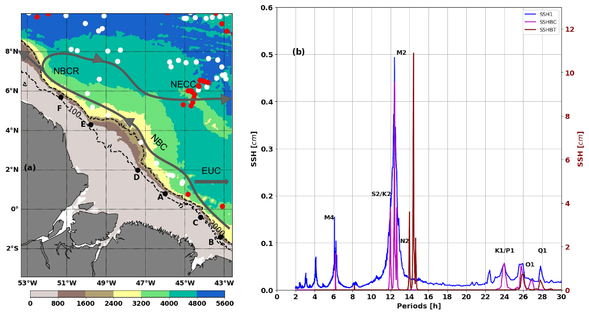
Figure 1(a) Model bathymetry and Argo profiles locations during MAMJJ (white dot) and ASOND (red dot). Points A, B, C, D, E, and F are internal tide generation sites mentioned in Magalhaes et al. (2016). Dashed blacks contours are 100 and 2000 m isobaths. Solid grey contours are NBC, NBCR, and NECC pathways, and EUC position is presented by a grey arrow. (b) SSH frequency spectra based on the 9.5 month (March to December) hourly signal of the coherent barotropic tides (SSHBT, brown), coherent baroclinic tides (SSHBC, magenta), and residual between the full SSH and SSHBT (SSH1, blue). The brown spectrum refers to the right scale and is shifted by 2 h for clarity. The spectra are averaged offshore of the 100 m isobath.
Our work is done as part of a project related to the future SAR-interferometry wide-swath altimeter mission SWOT (Surface Water and Ocean Topography). SWOT is designed to provide global 2D SSH observations for the spatial scale down to the sub-mesoscale of 15–30 km (Fu and Ferrari, 2008). The primary objective of the SWOT mission is to fill the gap in our knowledge of the 15–150 km 2D quasi-geostrophic ocean mesoscale and sub-mesoscale circulation determined from SSH (Fu et al., 2009; Fu and Ubelmann, 2014; Morrow et al., 2019). As with Jason-class along-track altimeter missions, SWOT is also specifically designed to observe the major ocean tidal constituents. SWOT should provide the first 2D SSH observations of the generation, propagation, and dissipation of internal tides and their interaction with the changing ocean stratification and circulation. In order to derive surface geostrophic currents (balanced motion) from the observed SSH gradients, a highly accurate prediction and correction of the SSH fluctuations due to non-geostrophic (unbalanced motion) high-frequency and internal wave motions are required, including barotropic tides and both coherent and incoherent internal tides. To date, the high-frequency barotropic tide is fairly well known from altimetry and models (Stammer et al., 2014; Carrère et al., 2021). The big challenge concerns the predictability of the internal gravity waves (IGWs) and baroclinic tides (Dushaw et al., 2011; Ray and Zaron, 2016; Zhao et al., 2016; Savage et al., 2017; Arbic et al., 2018). One of the key concerns in deriving surface geostrophic currents from altimetry is the spatial transition scale at which balanced motions dominate over unbalanced motions (Qiu et al., 2018). A second objective of this paper addresses the SSH structure in the Amazon shelf region, specifically on the geographical distribution of coherent and incoherent SSH, the variances they induce at different wavelengths, and the spatial “transition” scale. We are specifically interested in their variability from MAMJJ to ASOND.
Our study is based on a high-resolution ocean numerical model presented in Sect. 2. Section 2 is also dedicated to Argo and altimetric data used for the model validation and to the method of separating barotropic and baroclinic tides. The model is validated over the MAMJJ and ASOND seasons in Sect. 3 where the contrasting EKE characteristics are explored. The generation, propagation, and dissipation of the coherent internal tide M2 are presented in Sect. 4, along with some snapshots of the baroclinic flux and currents that illustrate the interaction of the internal tide with the circulation for each season. The SSH characteristics are analysed in Sect. 5. A summary of the paper is given in Sect. 6. The paper ends with Sect. 7 on discussion and perspectives.
2.1 Numerical model
The numerical model used in this study is NEMOv3.6 (Nucleus for European Modeling of the Ocean, Gurvan et al., 2019). The model domain covers the tropical Atlantic basin, and consists in a three-level, two-way embedding of: a ∘ grid covering the tropical Atlantic between 20∘ S and 20∘ N, a ∘ grid covering the western part of the basin (∼ 9 km resolution, from 15∘ S to 15∘ N, 55 to 30∘ W), and a ∘ grid (∼ 3 km resolution) covering the vicinity of the mouth of the Amazon (from 3.5∘ S to 10∘ N, from 53 to 42.5∘ W; for more details see Ruault et al., 2020). All three domains have 75 levels discretized on a Z* variable volume vertical coordinate, and 24 of the levels are within the upper 100 m. They are coupled online via the AGRIF library in two-way mode (Blayo and Debreu, 1999; Debreu, 2000). A third-order upstream biased scheme (UP3) with built-in diffusion is used for momentum advection. Laplacian isopycnal diffusion coefficients of 300, 100, and 45 m2 s−1 are used as tracers from the coarse to higher-resolution grid. A time-splitting technique is used to solve the free surface, with the barotropic part of the dynamical equations integrated explicitly. Atmospheric fluxes are from DFS5.2 (Dussin et al., 2016). The Amazon River discharges are based on the interannual time series from the So-Hybam (2019) hydrological measurements. The ∘ model is forced at its open boundary by the tidal potential of the nine major tidal constituents (M2, S2, N2, K2, K1, O1, Q1, P1, and M4) as defined by the global tidal atlas FES2012 (Finite Element Solution, Carrère et al., 2012). The ∘ model is initialized and forced at the lateral boundaries with daily velocity, temperature, salinity, and sea level from the MERCATOR GLORYS2V4 ocean reanalysis (http://marine.copernicus.eu/documents/PUM/CMEMS-GLO-PUM-001-025.pdf, last access: January 2019). The General Bathymetric Chart of the Oceans (GEBCO) bathymetry (Weatherall et al., 2015) was interpolated on each of the three nested grids. Figure 1a shows the domain and model bathymetry for the ∘ horizontal grid. Increasing the model horizontal resolution from to ∘ leads to more intense and realistic barotropic tide energy conversion to baroclinic tides (Niwa and Hibiya, 2011, 2014). The model was run over the period 2000–2015. In this study, we concentrate our analysis on hourly instantaneous output from the high-resolution grid stored from 15 March to 31 December 2015. A twin configuration of the model was run without the tidal forcing to allow spectral comparisons of the SSH with and without tides. More validations of the model are available in Ruault et al. (2020).
2.2 Observations: Argo potential density and altimetric SSH
Model validation was performed by comparing model outputs with observations. The model potential density and stratification were compared to the CORA (Coriolis Ocean Dataset for Reanalysis; Szekely et al., 2019) dataset. We benefited from the preprocessing data done by Barbot et al. (2021) on CORA version 4.3 data to gather density profiles. CORA data were co-located in time and space with model outputs. For 2015, most of the CORA data were Argo float observations in our model area (see location in Fig. 1). Altimetry data are from the daily mean ∘ × ∘ AVISO “global ocean gridded L4 sea surface heights and derived reprocessed variables (Copernicus climate service)”. Zonal and meridional geostrophic currents for the year 2015 were used to validate the EKE of the model. AVISO SSH and current anomalies are relative to a 1993–2012 mean. Along-track 1 Hz SARAL/AltiKa sea level anomaly altimetric observations for the period 2013–2014 were used to validate the model SSH wavenumber spectrum. With its Ka-band, the SARAL altimeter has a lower noise level and gives access to smaller horizontal scales compared to the Jason series Ku-band altimeter (Verron et al., 2015). Altimetric data are all available on the website https://www.aviso.altimetry.fr (last access: January 2022). The barotropic and coherent baroclinic SSHs are validated by comparison, respectively, to FES2012 and to Ray and Zaron (2016) internal tide SSH estimations based on altimetric observations.
2.3 Barotropic and baroclinic tide separation
Barotropic and baroclinic tides must be clearly separated to derive a correct internal tide energy budget. Baroclinic pressure and horizontal velocity are commonly defined as the difference between the total field and the depth-averaged field in a stratified ocean. This definition proposed by Kunze et al. (2002) can lead to spurious barotropic flux within the baroclinic flux (Kurapov et al., 2003). Kelly et al. (2010) renewed the Kunze et al. (2002) definition by adding a pressure–depth-dependent correction term to account for isopycnal heaving due to movement of the free surface. Much better physical representations of the baroclinic energy fluxes are obtained by considering the barotropic tide as the fast mode (mode 0) and the baroclinic tide as the sum of the baroclinic modes in a normal-mode decomposition (Kelly, 2016; Gill, 2003). Nugroho (2017, chap. 6) used the vertical mode decomposition but replaced the surface rigid lid condition with a surface pressure condition based on the SSH free surface, in order to keep the fast (barotropic) mode in the set of mode solutions of the Sturm–Liouville problem. The free-surface boundary condition eliminates unphysical energy flux arising from the rigid lid condition and gives similar barotropic to baroclinic energy conversions as Kelly et al. (2010) and Kelly (2016). We, therefore, used the Nugroho (2017) method to analyse the coherent internal tide and followed the Kelly et al. (2010) methodology to describe the baroclinic flux over short periods (see Sect. 4).
In practice, to carry out the vertical mode decomposition, we solve the eigenfunctions for 10 modes at each point of the model using the local mean stratification over the analysed periods (the entire period, March to December, or the seasons MAMJJ and ASOND). We then fit the U eigenmodes to each harmonic constant of the 3D velocity and pressure fields and used the modal amplitudes and phase in the energy analysis (see Eqs. 1 to 5 in Sect. 4). This provides the description of the barotropic tide (mode 0) and the coherent baroclinic tide that can be analysed for each mode or as the sum of the nine baroclinic modes. The M2 wavelength varies spatially and temporally between 90–125 km for mode 1 and 12–15 km for mode 9 (not shown). The horizontal resolution of the model allows us to solve for the first eight modes (Buijsman et al., 2020; Soufflet et al., 2016). However, the energy of the internal tide for baroclinic modes higher than mode 2 is so weak that taking into account two, seven, or nine baroclinic modes does not change our results (not shown).
3.1 Numerical tidal solution validation
We first evaluated the ability of the model to correctly simulate the barotropic and baroclinic tide. For this purpose only, the barotropic and baroclinic tides are evaluated over the entire simulation period from March to December (Figs. 1b and 2). The frequency spectra in Fig. 1b confirm that M2 is the dominant tide component for both barotropic and baroclinic modes. The modelled M2 barotropic and baroclinic tides were compared to the M2 barotropic tide from the hydrodynamic model assimilating altimeter data FES2012 from Carrère et al. (2012) and also to the M2 baroclinic tide from altimetry observations from Ray and Zaron (2016).
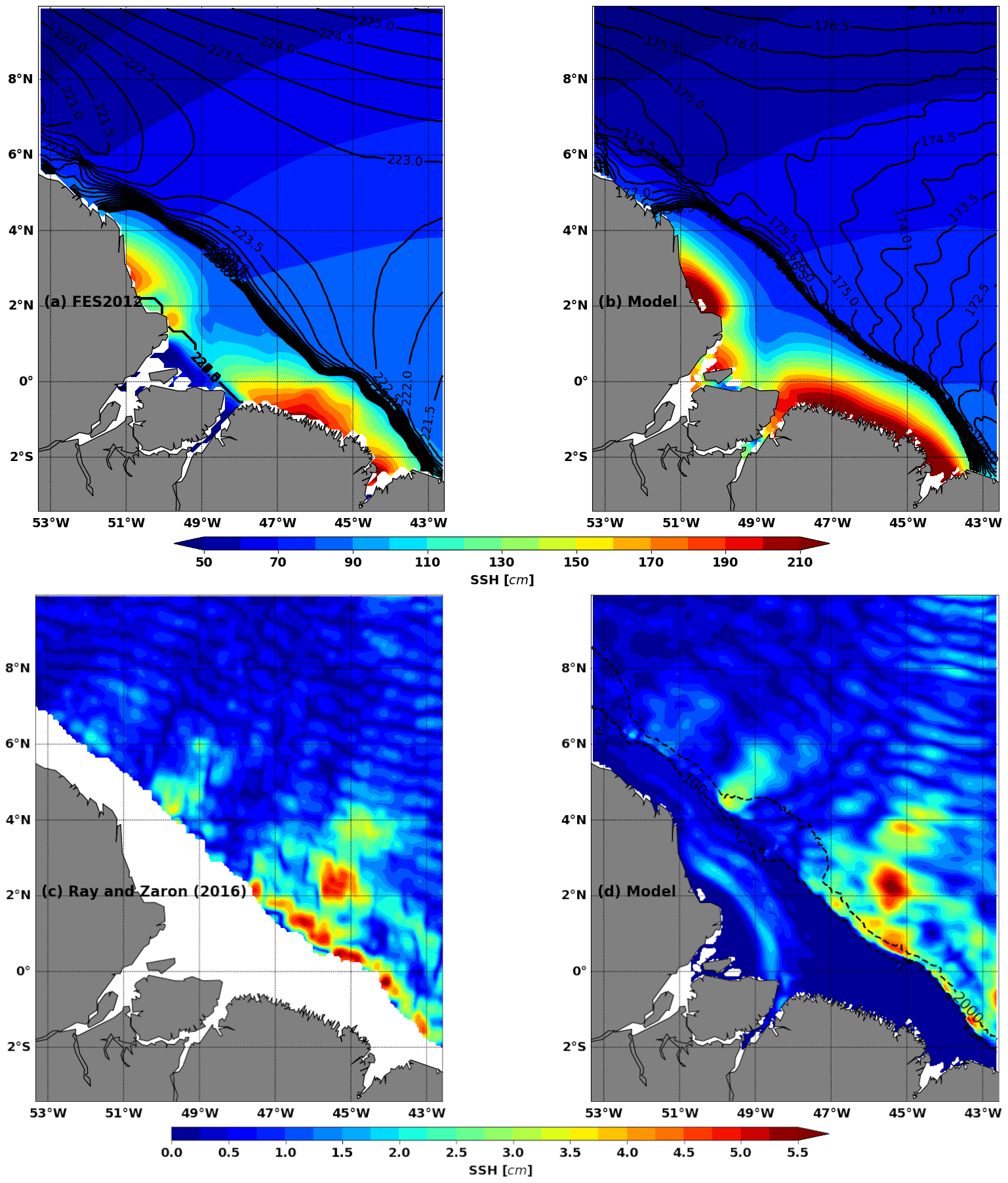
Figure 2(a, b) M2 coherent barotropic SSH from (a) FES2012 (Carrère et al., 2012) and (b) the model. (c, d) M2 coherent baroclinic SSH from (c) altimetry by Ray and Zaron (2016) and (d) the model. Amplitude is in colour (unit: centimetres), and the phase is in solid black contours. Dashed blacks contours are 100 and 2000 m isobaths. The models are based on the 9.5-month hourly output.
The barotropic tide evolves freely in the model after it has been forced at its lateral boundaries by FES2012. The resulting modelled M2 barotropic is maximum near the northwest and southeast of the Amazon mouth because of the landward propagation and convergence of the barotropic tide coming from the open ocean (Fig. 2b). Even though the M2 modelled barotropic SSH is stronger than FES2012 (Fig. 2a), the model and FES2012 agree. The differences with FES2012 might come from different bathymetry and friction coefficients (see Le Bars et al., 2010, for sensitivity study) or the difference in the river boundary conditions (closed in our simulation whereas tide penetrates into the Amazon for FES2012). The comparison between model and observations is also satisfactory for M2 baroclinic SSH (Fig. 2c and d). M2 internal tide amplitudes reach 5 cm in the region. Sites E and F are distinguished north of 2∘ N, while to the south the internal tide is at a maximum along the 100 m isobath. It is not surprising that the model and observations are not identical point by point, especially since the baroclinic SSH of Ray and Zaron (2016) is based on 20 years of altimetry observations.
3.2 Validation of the simulated regional circulation: the contrast between MAMJJ and ASOND
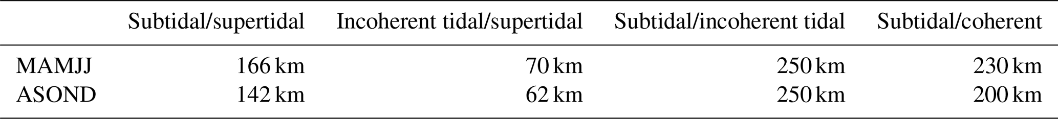
In this subsection, we illustrate the contrasts in ocean conditions (circulation and stratification) between MAMJJ and ASOND in the model. The surface current, the EKE, and density profiles are validated by comparison with AVISO and Argo observations. The 5-month “seasons” of MAMJJ and ASOND correspond to 1752 h covering the periods shown in Table 1. The MAMJJ shift of 1 week in August is necessary to have the same number of spring and neap tide cycles, which is necessary for the comparison of tidal harmonics.
3.2.1 Mean current and EKE during MAMJJ and ASOND
First, 25 h running means were performed to separate tide and high frequency from the low-frequency mesoscale variability in the model. Then EKE was evaluated using the anomaly of the 25 h running mean current relative to the mean current from March to December. During MAMJJ, the current is weak, the NBC is trapped along the coast, and the EKE is between 900–1200 cm2 s−2 (Fig. 3a). During ASOND, the NBC is wider and more intense, the NBC retroflection (NBCR) and the eastward current NECC are easily distinguished, and the EKE values exceed 2000 cm2 s−2 along the NBCR–NECC pathways (Fig. 3b). The behaviour of the surface currents between MAMJJ and ASOND corresponds to the seasonal description given in the introduction. Figure 3c and d show EKE in MAMJJ and ASOND for the year 2015 from the AVISO data. They confirm the EKE contrasts in our model, although the model and AVISO are quite different, mainly around the Amazon shelf break (2–4∘ N, 50–47∘ W). The sources of these differences are multiple, including the horizontal resolution (∘ for AVISO and ∘ for NEMO), the reference period for the calculation of the mean current used to calculate the anomalies (1993–2012 for AVISO, 2015 for NEMO), the nature of the currents (geostrophic for AVISO, total for NEMO) and the processing of the altimeter signal at the limit of the continent, where internal gravity wave residuals are still present in AVISO-mapped data (see Fig. 10 in the following), which could be the reason why AVISO is at a maximum around the Amazon shelf break (Fig. 3c and b).
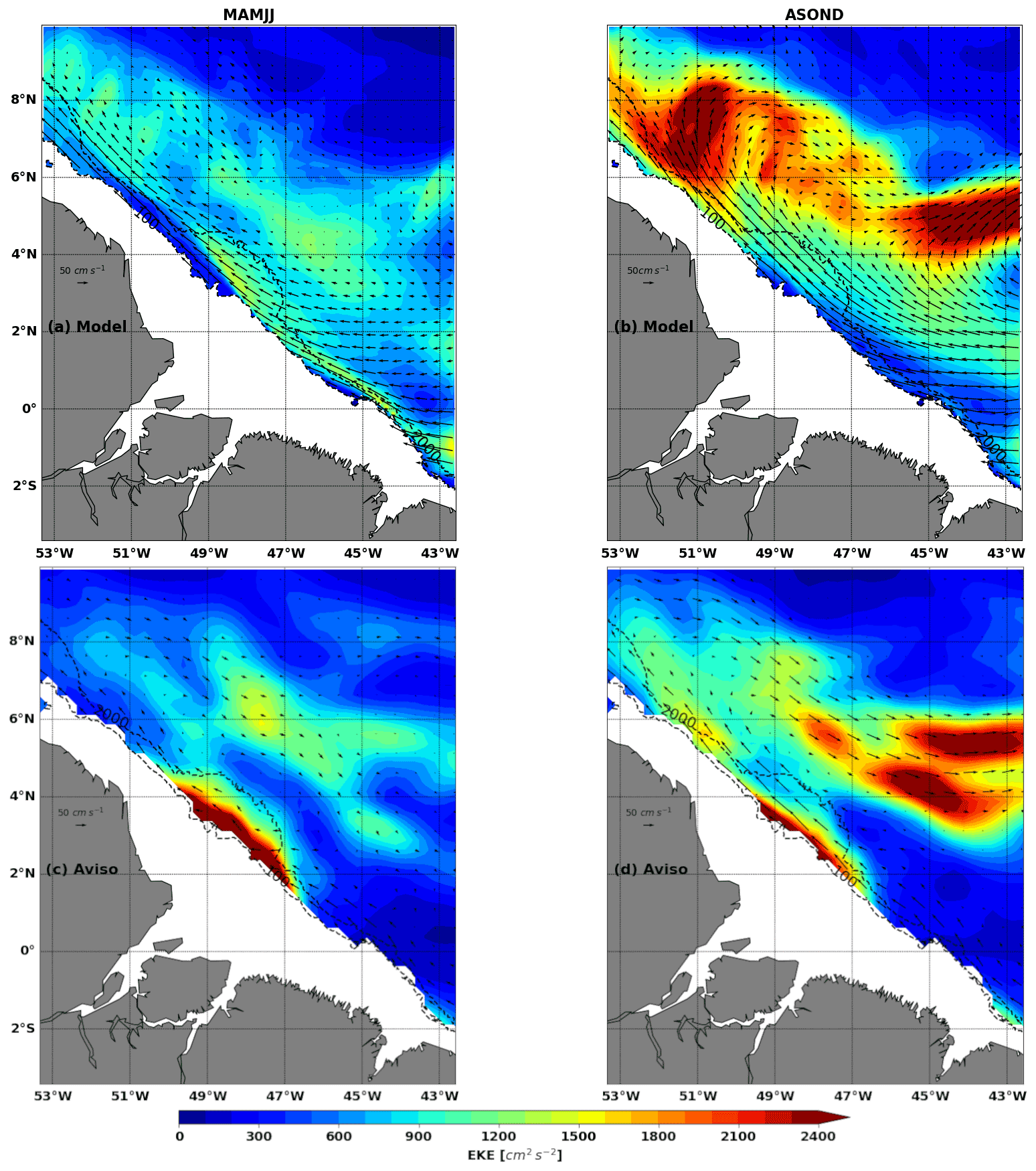
Figure 3(a, b) Model mean surface EKE (colours, units: cm2 s−2) and current (arrows, units: cm s−1) during (a) MAMJJ and (b) ASOND. (c, d) AVISO mean surface EKE during (c) MAMJJ and (d) ASOND. Dashed black contours are 100 and 2000 m isobaths. Bathymetry less than 100 m is masked.
3.2.2 MAMJJ and ASOND stratifications
About 50 Argo vertical profiles of potential density were selected between March and December 2015. The selection criterion was the stability of the Brunt–Väisälä frequency (hereafter N) in the first 1000 m of depth (see Barbot et al., 2021, for more details on the selection of Argo).
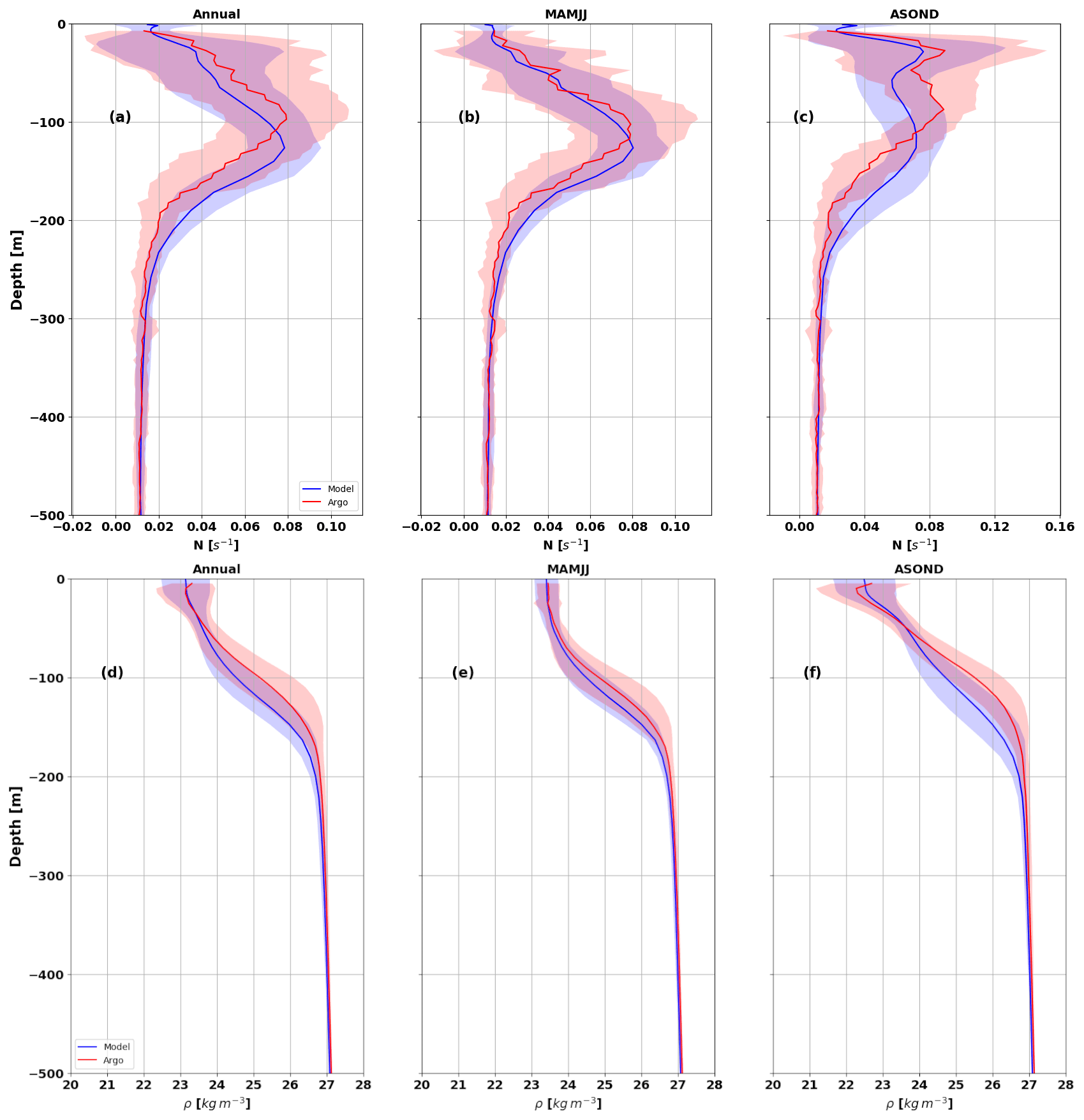
Figure 4Mean vertical profiles from Argo (red) and model (blue) during (a, d) March to December 2015 (annual) and (b, e) MAMJJ and (c, f) ASOND. (a–c) Brunt–Väisälä frequency (N, units: s−1). (d–f) Potential density (units: kg m−3). The blue and red envelopes are the standard deviation. See Fig. 1 for Argo profile location. Model profiles are collocated in time and space with Argo profiles.
The model and observations are collocated in time and space. The mean potential density profiles from March to December (annual, in Fig. 4), and over the MAMJJ and ASOND seasons, are presented in Fig. 4 with the corresponding N vertical profiles. The Argo profiles are in red, and those of the model in blue. The blue and red envelopes are the standard deviation.
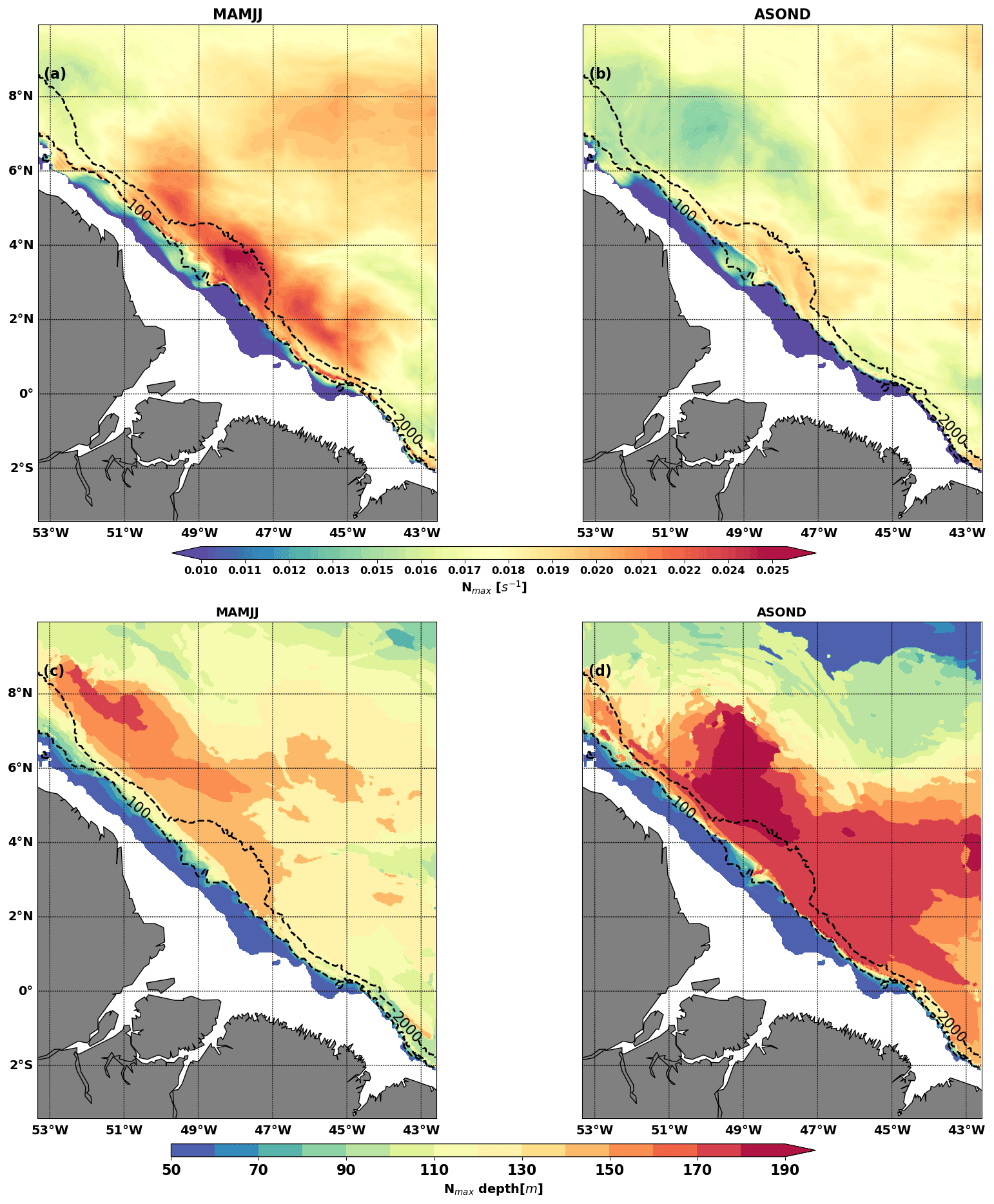
Figure 5(a, b) Nmax value (units: s−1) during MAMJJ (a) and (b) ASOND. (c, d) Pycnocline depth (depth of Nmax, units: m) during MAMJJ (c) and (d) ASOND. The Nmax value and depth were deducted from the mean potential density over each season. Dashed black contours are 100 and 2000 m isobaths. Bathymetry less than 50 m is masked.
Overall, the model reproduces the vertical and temporal variations in the potential density and N fairly well (Fig. 4). More than half of the vertical profiles concern the MAMJJ season (Fig. 1a), so that the annual profiles are closer to the stratification during this season (Fig. 4a–b and d–e). The vertical profiles of N (Argo and model) are characterized by two maxima (Nmax) in ASOND (Fig. 4c). The shallower is located in the first 50 m of depth and is associated with very light water of the Amazon plume (Fig. 4f). The presence of this near-surface Nmax will have an impact on the modal structure of the internal tide and certainly impacts the internal wave regime according to Gerkema (2003). We do not address the issue of the internal wave regime in this study. Vertical sections (not shown) indicate that the internal tide interacts first with the base of the pycnocline around the depth of the second peak of N. Thus, to differentiate MAMJJ from ASOND, and following Barbot et al. (2021), we will use the deeper Nmax as the proxy of the pycnocline.
The first 50 m of depth was not taken into account when determining the depth of Nmax and its intensity at each valid point of the model for the MAMJJ and ASOND seasons (Fig. 5). Nmax is stronger in MAMJJ compared to ASOND (Fig. 5a and b), so ocean stratification conditions during ASOND are more favourable for internal tide scattering (Gerkema, 2001). Except north of 2∘ N, the Nmax depth is less than 140 m in MAMJJ (Fig. 5c). During ASOND, the NBC retroflection splits the domain in two. The pycnocline deepens by about 50 m and reaches 170 to 190 m in the area delimited by the NBC and its retroflection (Fig. 5d). Offshore the pycnocline gradually rises, and the NBCR creates a kind of pycnocline gradient that could limit the propagation of the coherent internal tide (Li et al., 2019). The deepening of pycnocline in ASOND is favourable to the generation of mode 1 internal tide and less favourable to the generation of higher modes (Barbot et al., 2021).
Table 1 summarizes the circulation and stratification contrasts between MAMJJ and ASOND. MAMJJ is the season of low current, low EKE, and a shallower and stronger pycnocline with weak spatial gradient. In ASOND, the currents are stronger, the retroflection is well developed, the EKE is strong, and the pycnocline is deeper and weaker with stronger horizontal gradient.
Table 1Circulation and stratification characteristics during the MAMJJ and ASOND seasons.

4.1 M2 coherent internal tide for MAMJJ and ASOND: generation, propagation, and dissipation
Assuming that the energy tendency and nonlinear advection are small, the barotropic and baroclinic tide energy budget equations reduce to a balance between the conversion rate (CVR), the divergence of the energy flux, and the dissipation (Buijsman et al., 2017; Tchilibou et al., 2020) as shown by the equations below.
with
In these equations, bt and bc indicate the barotropic and baroclinic tides, U(u,v) is the horizontal velocity, P is the pressure, F is the energy flux, D is the dissipation term, H is the bottom depth, η is the surface elevation, and gradh and divh are the horizontal gradient and divergence operators. The overbar indicates an average over a tidal period. CVR appearing in the barotropic (Eq. 1) and baroclinic (Eq. 2) energy budget equations determines the amount of barotropic tide energy converted into baroclinic tides. The baroclinic (Fbc, Eq. 5) and barotropic (Fbt, Eq. 4) fluxes respectively provide information on baroclinic and barotropic tide propagation pathways. We derived the dissipation D from Eqs. (1) and (2). Note that D is more of a proxy of the real dissipation because it may also include energy loss to numerical dissipation (Nugroho et al., 2018).
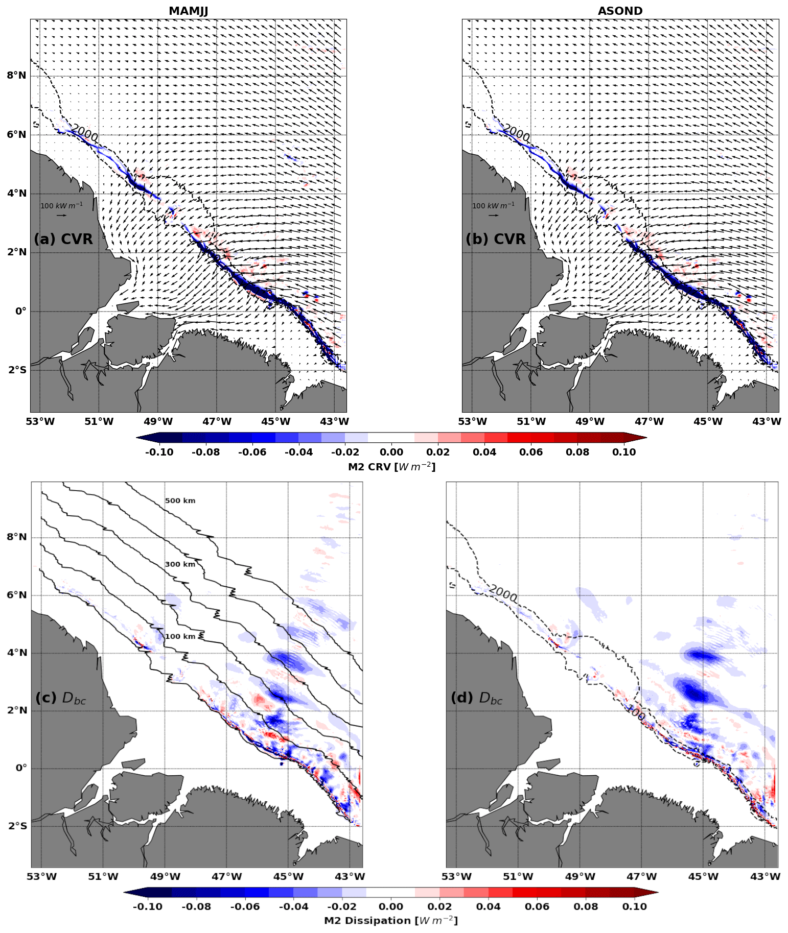
Figure 6Top: M2 conversion rate (CVR, colour, units: W m−2) and barotropic flux (Fbt, arrows, units: W m−1). Bottom: dissipation of M2 coherent (colours, D, units: W m−2). Left column is for MAMJJ (a, c) and right column is for ASOND (b, d). Dashed black contours are 100 and 2000 m isobaths. The black solid contours are parallels to the 100 m isobath drawn every 100 km and along which the integrations are performed for Fig. 8.
For MAMJJ (Fig. 6a, vectors) and ASOND (Fig. 6b, vectors), the M2 barotropic energy fluxes are quasi-identical, as only a small fraction of barotropic energy loss is due to internal tide generation (compared to bottom friction), and the resulting change in the conversion rate is itself a small fraction of the total. The M2 barotropic energy flux originates from the southeastern open ocean and propagates towards the continental shelf. Initially directed towards the northwest, the fluxes gradually turn southward as they cross the shelf and converge towards the mouth of the Amazon River and Para River. The cross-shelf barotropic energy fluxes will be eroded through dissipation (Dbt) or through the generation of internal tides (CVR) according to Eq. (1), until full extinction. North of 4∘ N in the NBC retroflection and NBC ring area, the barotropic tide flux decreases, likely because a large part was diverted toward the Amazon shelf.
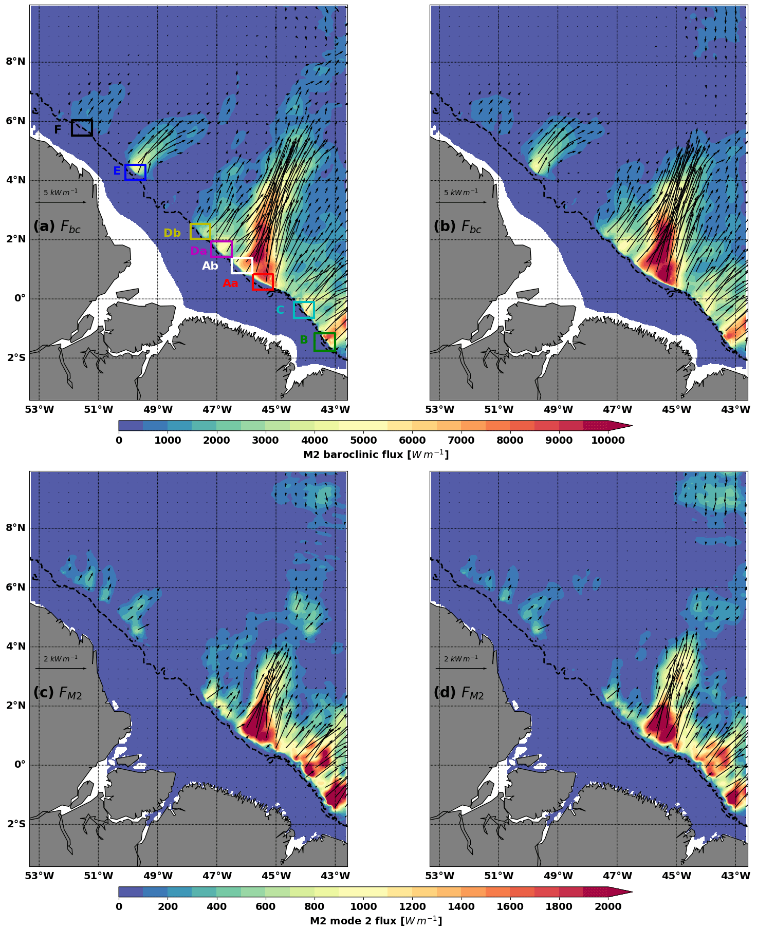
Figure 7M2 total (a, b) and mode 2 (b, d) baroclinic flux (Fbc, colours and arrows, units: W m−1). Left column is for MAMJJ (a, c) and right column is for ASOND (b, d). Dashed black contours are 100 and 2000 m isobaths. Boxes delimit eight hotspots of internal tide generation.
Internal tide generation occurs along the shelf break (Fig. 6a and b, negative values and blue colour shading) between the 100 and 1000 m isobaths, with some exceptions until 1800 m (Fig. 6a and b). Note that the positive conversion rate in Fig. 6 (energy directed from the baroclinic tide towards the barotropic tide) can occur when the phase difference between the baroclinic bottom pressure perturbation and the barotropic vertical velocity exceeds 90∘ (Zilberman et al., 2011). Typically, this will happen at some distance of the generation site, at non-flat bottom locations, as the phase speed of the baroclinic tides is much slower than that of barotropic tides, making the phase difference vary quickly in the propagation direction. As noted in Fig. 2, internal tide generation is stronger south of the Amazon cone (situated between 2–4∘ N, 50–47∘ W) than north of it. During MAMJJ, the total M2 conversion rate integrated over the entire model domain is 5.05 GW, including 3.66 GW for mode 1, 1.06 GW for mode 2, and 0.21 GW for mode 3. During ASOND, the total remains the same (5.08 GW), but there is more in mode 1 than in MAMJJ (3.92 GW) and less in modes 2 and 3 (0.93, 0.13 GW). This is explained well since the pycnocline is closer to the surface during MAMJJ than during ASOND. A detailed analysis of the conversion rate in the boxes surrounding sites A to F is presented in the appendix (see Fig. 7 for location and Table A1 in Appendix A for coordinates). The hotspots of internal tide generations are located in A (Aa + Ab) and B sites in good agreement with Magalhaes et al. (2016). Site B, on the other hand, is the site where the conversion to baroclinic tide is the least effective due to the orientation of the barotropic flows (see P1 in Table A1).
After generation, M2 internal tide mainly propagates to the open ocean in the northeast direction (Fig. 7a and b). The maximum propagation occurs from sites A and B, although south of 2∘ N, the M2 internal tide propagates from the entire coastline including sites D and C. The baroclinic flux from these latter sites then contributes in part to strengthening the baroclinic flux from A. North of 2∘ N, internal tides propagate selectively from points E and F. The mode 1 baroclinic flux is similar to the total (not shown), and mode 2 is about 10 times weaker than the total (Fig. 7c and d) south of 2∘ N. Figure 7 shows significant divergence in the propagation of the M2 coherent internal tides between MAMJJ and ASOND. In particular, mode 1 and mode 2 baroclinic fluxes from A propagate further north during MAMJJ than during ASOND. During MAMJJ, the baroclinic flux reaches 8∘ N while it is largely blocked at 6∘ N during ASOND. The arrest of the propagation of the baroclinic flux from A could suggest at first order a significant increase in dissipation of the coherent M2 between the two seasons.
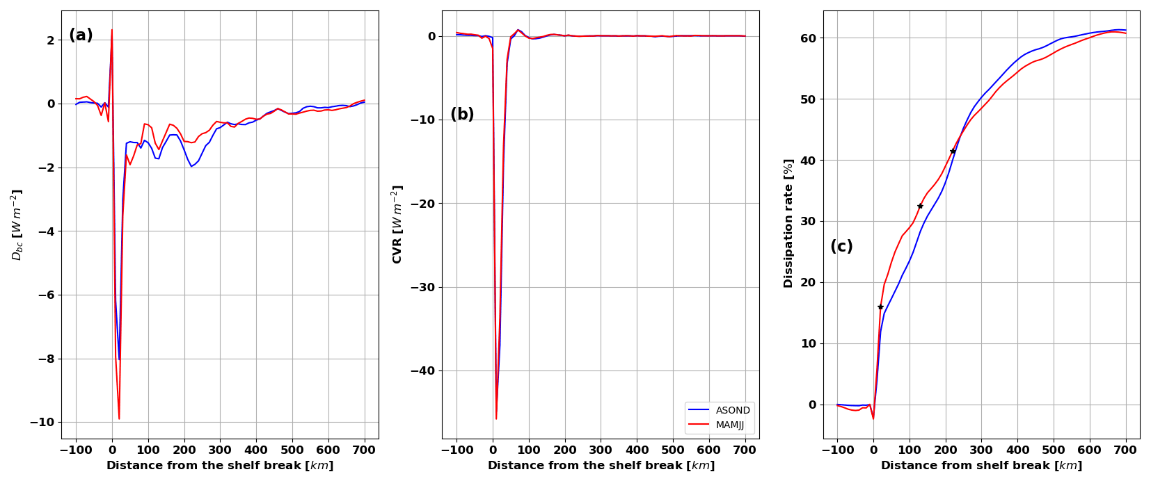
Figure 8(a) Dbc (units: W m−2), (b) CVR (units: W m−2), and (c) dissipation rate (%) as a function of distance from the continental shelf break. CVR and Dbc are integrated every 10 km from the shelf break. The dissipation rate is the ratio between the cumulative sum of Dbc and the sum of CVR within the first 50 km from the shelf break. ASOND is in blue and MAMJJ is in red. The black stars are the locations of the three peaks of maximum dissipation.
A proxy of the dissipation is given in Fig. 6c and d as the residual between the conversion rate and the divergence of the baroclinic flux. Although it does not take into account non-linear terms, it is quite revealing of the coherent internal tide dissipation. Most of the dissipation occurs locally in a wave-like pattern parallel to the shelf break contours from E to B, with wavelengths between 90 and 120 km (Fig. 6c and d). The dissipation maps indicate local dissipation on the shelf break near site F, but not offshore. Contrary to what could have been an explanation for the flux blocked at 6∘ N, there are no particular dissipation structures apparent during ASOND beyond 4∘ N. To further compare the dissipation over the two seasons, we integrated it every 10 km along sections parallel to the shelf break (here the 100 m isobath), and we present it as a function of the distance to the shelf break in Fig. 8a. The maximum dissipation occurs 20 km offshore, and it is separated from a much weaker second peak located 110 km offshore and a third peak at 200 km offshore (Fig. 8a). These are the same distances that separate the negative patches of dissipation in Fig. 6c and d.
The M2 conversion rate is integrated in the same way as the dissipation, having a maximum at 10 km distance from the shelf break and a zero crossing at 50 km from the shelf break (Fig. 8b). The 50 km distance was considered the boundary between local dissipation on the shelf break including the generation sites from A to F and the remote dissipation in the open ocean. From the dissipation and conversion rate curves in Fig. 8a and b, we defined the dissipation rate as the ratio between the cumulative sum of the dissipation and the conversion rate within the first 50 km from the shelf break. During MAMJJ, 23 % of the generated internal tide dissipates locally on the shelf break, and the local dissipation rate decreases to 17 % in ASOND (Fig. 8c). The local dissipation rates found for the entire coastline are of the same order and vary in a similar way between MAMJJ and ASOND, as shown in the box analysis (see Table A2). The dissipation rates at the three dissipation peaks (beams; see star in Fig. 8c) are 16 %, 32 %, and 41 % during MAMJJ and 11 %, 28 %, and 40 % during ASOND. The second and third peaks account for the remote dissipation. They show a slight increase in the dissipation rate from the second to the third beams during ASOND (12 %) compared to MAMJJ (9 %). The remote dissipation rates are about 50 % for both seasons at 300 km from the shelf break (Fig. 8c). Thus, there is no drastic increase in dissipation from the MAMJJ season to ASOND, and thus, the dissipation of the coherent M2 modes cannot explain all the differences in baroclinic fluxes. A more detailed exploration is performed in the following section to analyse the change of the baroclinic flux from MAMJJ to ASOND.
4.2 Detailed analysis of the baroclinic flux and the current: internal tide interactions with the circulation
The internal tide generated on the Amazon shelf propagates through a complex environment of strong boundary currents (NBC, NECC, EUC), eddies, and salinity plumes associated with strong frontal structures and density gradients. It is not excluded that changes in oceanic conditions from MAMJJ to ASOND have an impact on the trajectory of the internal tides through the interaction between the internal tide and the background circulation (eddies, current, or stratification). To more precisely investigate the internal tide interactions with the circulation, we make the choice to leave aside the harmonic analysis approach, which does not allow us to depict short-term changes in the internal tide propagation characteristics. Instead, we make use of time filtering over a 25 h period, which provides a fair separation of tidal and non-tidal processes, at the sacrifice of individual tidal constituent diagnostics, leaving the neap and spring tide modulation in the filtered tidal signal. In Fig. 9, the vertically integrated baroclinic flux, the relative vorticity and the current along the 1025 kg m−3 isopycnal are presented together for some typical dates which summarize the conditions during MAMJJ and ASOND well (videos showing the daily propagation of internal tides are provided in the Supplement). As expected, the 25 h mean eliminates the tidal signal in the currents while preserving the background and mesoscale circulation (Fig. 9). The 25 h averaged internal tide flux (computed from the hourly low-pass-filtered simulated currents and pressure and averaged over 25 h) now refers to the total baroclinic flux; i.e it includes all the modelled baroclinic modes and tidal constituents. Even though the internal tide signal is dominated by mode 1 of M2, the stronger higher modes 2 and 3 during MAMJJ could add smaller scales to the baroclinic signal. The isopycnal 1025 kg m−3 was chosen because it is representative of the thermocline spatial and temporal variability in the area. It should also be noted that in this region, several eddies have a reduced surface signature (Garraffo et al., 2003), and the isopycnal 1025 kg m−3 crosses the cores of the main currents.
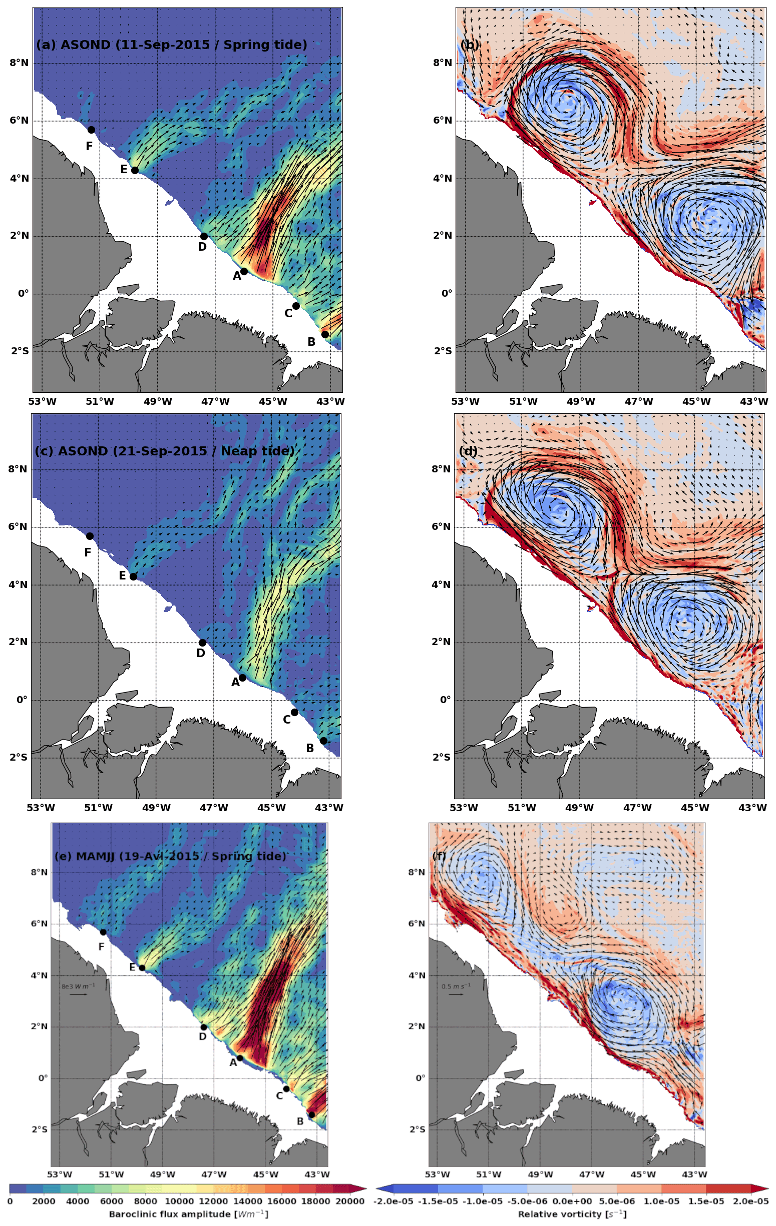
Figure 9Examples of 25 h mean snapshots of depth-integrated baroclinic flux (colours and arrows, left, units: W m−1), relative vorticity along the 1025 kg m−3 isopycnal (colour, right, units: s−1), and horizontal velocity along the 1025 kg m−3 isopycnal (arrows, right, units: m−1) on (a, b) 11 September 2015 spring tide during ASOND, (c, d) 21 September 2015 neap tide during ASOND, and (e, f) 19 April 2015 spring tide during MAMJJ. Bathymetry less than 100 m is masked.
During ASOND, the very intense currents delimit a frontal line with a steep pycnocline slope. Along the 1025 kg m−3 isopycnal, we can also distinguish anticyclonic eddies that skim the coast (Fig. 9b and d). The signature of these eddies is intensified in the upper ocean, but they have a significant barotropic signature too. On 11 September 2015, a day of spring tide during ASOND, the baroclinic flux originating from A initially directed towards the northeast turns towards the east between 4–6∘ N where the current and the circulation at the edge of the anticyclone are very intense and directed almost horizontally towards the east (Fig. 9a and b). The baroclinic flux coming from D divides in two, and the first part quickly merges with the baroclinic flux coming from A. The other part directed towards the northwest interacts with the front or the current around 5∘ N and turns to the northeast. Starting from E, the baroclinic flux keeps its initial direction for a few kilometres before being redirected east and merging with the baroclinic flux coming from D. The propagation of the baroclinic flux generated in F is almost inhibited by the anticyclonic circulation (Fig. 9a and b). On 21 September 2015, the current and eddies remain intense, and the baroclinic flux decreases because it is a neap tide day. The baroclinic flux of the different sites undergoes the deviations noted previously but is made up of more branches (Fig. 9c and d).
During MAMJJ, the currents are weaker and the eddies less intense and of smaller diameter (Fig. 9f). In Fig. 9e and f showing 19 April 2015, the baroclinic flux of A extends further offshore. It is almost not deflected by the ocean circulation, which is more southward (around 4∘ N) than in ASOND. Weak circulation and spring tide conditions are favourable for the propagation of the flux coming from F for this day (Fig. 9e), and the baroclinic flux and the eddy skimming the coast near F are in opposite directions.
According to Fig. 9, MAMJJ and ASOND are mainly distinguished by the intensification of the eastward deviation of the baroclinic flux by the circulation east of 45∘ W in ASOND. At sites D, E, and F, the internal tidal flux is subdivided into different branches, including a main eastern branch which sometimes merges with the baroclinic flux from a neighbouring site. Figure 9 also highlights the neap tide and spring tide modulation of the interactions between the internal tide and the background circulation. Thus, the harmonic analysis only captures the internal tide trajectories with the most occurrences over the analysed periods and selected frequency. The internal tides have not dissipated as one might think with regard to the M2 baroclinic flux M2 during ASOND (Fig. 6), but the interaction between internal tides and the background circulation induce ramifications and deviations of the baroclinic flux such that on average at M2 frequency there is no preferred propagation direction beyond 6∘ N during ASOND.
Since the differences between the M2 baroclinic fluxes of MAMJJ and ASOND are strongly linked to the interactions with the circulation, a fraction of the internal tide has become incoherent (non-phase-locked). The term incoherent is not limited to the internal tide; it also encompasses internal gravity waves (IGWs), which constitute a continuum of energy over a wide range of spatial and temporal scales. This study is conducted as part of a SWOT project, so we evaluate the incoherent components based on their SSH signatures.
As mentioned in the introduction, SSH from altimetric observations or models includes high-frequency unbalanced (non-geostrophic) components from the barotropic tides, from the coherent and incoherent internal tides, and from IGWs. Global model estimates of the barotropic tide are applied as a correction to altimetric SSH before the data are used for ocean circulation studies (e.g. FES2014, Lyard et al., 2021). New global coherent internal tide corrections are also becoming available (e.g. M2 SSH, Ray and Zaron, 2016). However any residual errors from these tide model corrections will remain in the corrected altimetric SSH data and pollute the calculation of balanced (geostrophic) currents from SSH altimetry observations. In the perspective of using SSH measurements including SWOT to study geostrophic (balanced) motion, it is important to understand what spatial and temporal scales are affected by these non-geostrophic components, so that adequate filtering can be applied to remove them for ocean circulation studies. This section addresses these scales for the Amazon region. To study the SSH variations, the hourly SSH of the tidal model is split as indicated by Eqs. (6) and (7).
SSHBT and SSHBC are respectively the coherent barotropic and baroclinic SSH, and they constitute mode 0 and the sum of the nine baroclinic modes remaining after projection on the vertical mode (see Sect. 2.3). They contain both the diurnal and semidiurnal tide components by which the model was forced. SSH1 corresponds to the usual processing of altimeter observations from which the barotropic tide correction is removed from the total SSH (Eq. 6). The coherent part of internal tides (SSHBC) is removed from SSH1 to obtain SSH2 (Eq. 7). SSH1 and SSH2 have similar low-frequency (here h−1) components, with the high frequency ( h−1) of SSH2 being the incoherent SSH (internal tide and IGWs).
To study the spatio-temporal scales of the coherent and incoherent SSH, spectral analyses are performed on SSHBC, SSH1, and SSH2. Before the fast Fourier transform (FFT) calculation, SSH is detrended and windowed with a Tukey 0.5 window, as previously done in Tchilibou et al. (2020). The spectra are integrated over different frequency bands. We consider the “subtidal” to be the periods above ( h−1), the “tidal” to be the periods between 28 and 11 h ( h−1 < h−1), and the “supertidal” to be the periods below 11h ( h−1). The sensibility to these cutoff frequency bands was tested without major changes to our results. The frequency band distribution is such that the intraseasonal and mesoscale low-frequency variations are contained in the subtidal band. The high frequency of tides and gravity waves is contained in the tidal and supertidal bands. A separate analysis of the SSH variations in the model without tides revealed that fluctuations associated with high-frequency atmospheric forcing can be neglected here (not shown).
5.1 Geographical distribution of the SSH temporal root mean square (rms) for different frequency bands
The frequency spectra of the total baroclinic tides, SSH1, are integrated at each point of the model to deduce the geographical distribution of the total (full, Fig. 10a and b), tidal-band (Fig. 10a and b), and supertidal-band rms (Fig. 10e and f) during both seasons: MAMJJ (Fig. 10, left) and ASOND (Fig. 10, right).
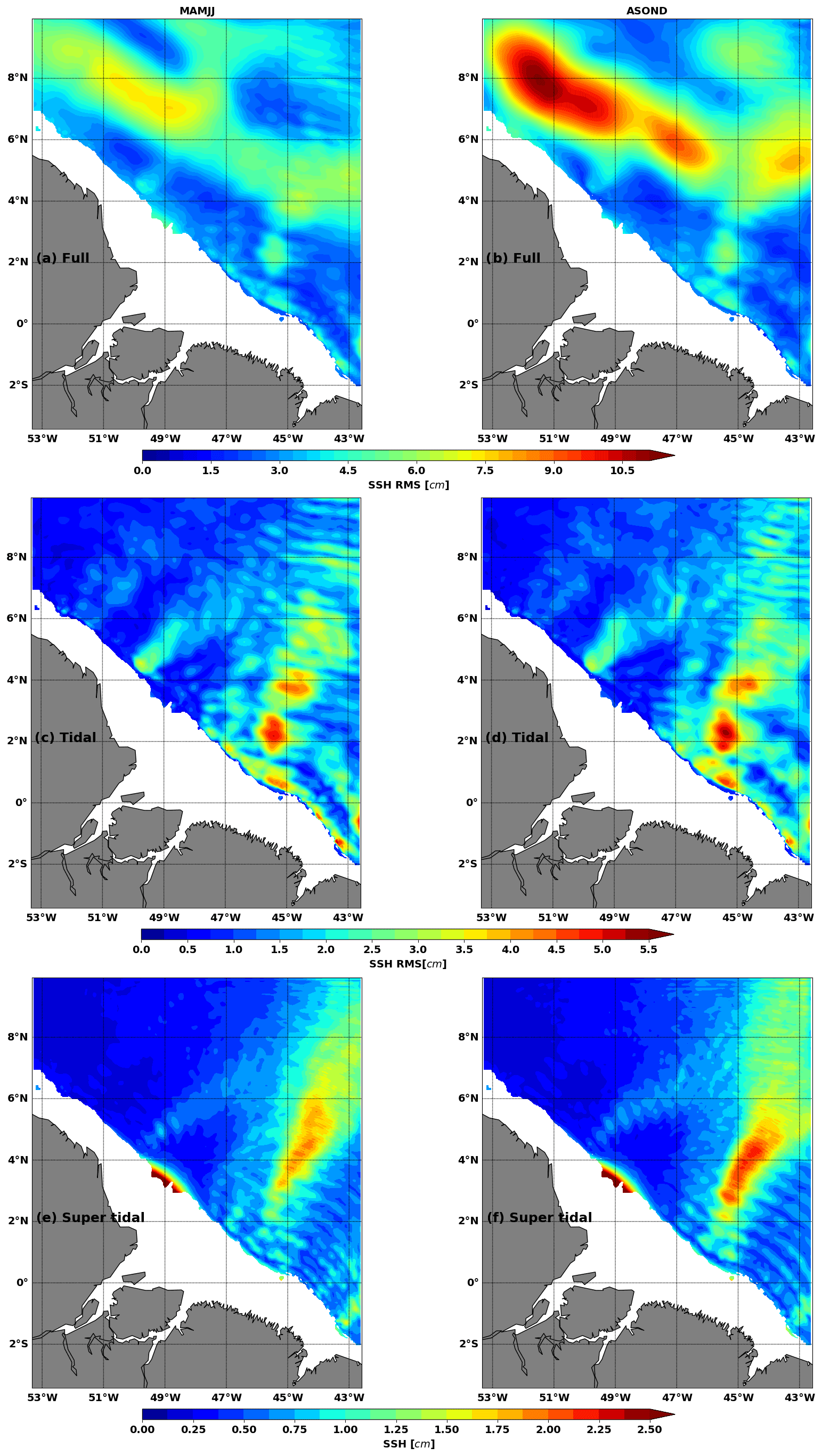
Figure 10Root means square (rms) of SSH1 for (a, b) all frequencies (full), (c, d) tidal frequencies ( h h−1), and supertidal frequencies ( h−1) during MAMJJ (a, c, e) and ASOND (b, d, f). SSH1 is the residual between the SSH and the coherent barotropic SSH (SSHBT); see Eq. (8). Units: cm. Bathymetry less than 100 m is masked.

Figure 11Root mean square of (a, b) SSHBC and (c, d) SSH2 for tidal frequencies during MAMJJ (a, c, e) and ASOND (b, d, f). SSHBC is the coherent baroclinic SSH, and SSH2 is the incoherent SSH defined as the residual between SSH1 and SSHBC; see Eq. (9). Units: cm. Bathymetry less than 100 m is masked.
For both seasons the maximum variations in SSH1 occur north of 6∘ N and west of 48∘ W (Fig. 10a and b) where the retroflection of the NBC takes place (Fig. 3). Along the NBCR–NECC, the rms is greater than 4 cm and the EKE is maximal (Fig. 3). These maxima are first due to the intraseasonal mesoscale variations in the SSH since the same geographic distribution is observed on the subtidal rms (not shown). The second contributor to the SSH maximum variability is the baroclinic tidal frequency (Fig. 10 10c and d) associated in particular with the semi-diurnal internal tide as expected from Figure 1b. In the area 4–6∘ N, 43–45∘ W for example, the full rms is on average 5 cm in MAMJJ and 7 cm in ASOND while the rms is about 3 cm for the tidal band over the two seasons. The eastern part of the basin is the most marked by baroclinic tidal variability (Fig. 10c and d)as already seen for M2 in Fig. 2d. Initially measuring about 100 km close to the coast, the wavelengths become smaller offshore. Judging by their number, the waves propagating from the coast to the open sea at supertidal frequencies are of wavelengths less than 70 km (Fig. 10f and e). At supertidal frequencies, the SSH rms increases by 1 to 2 cm along the internal tide path from site A (Fig. 10e and f). MAMJJ and ASOND are particularly distinctive in their maximum and the shape of the envelope around it.
SSH1 includes the coherent baroclinic SSH (SSHBC) and the incoherent SSH (SSH2, Eq. 7). The coherent part (Fig. 11a and b) and incoherent part (Fig. 11c and d) of SSH1 at tidal frequencies (Fig. 10c and d) are separately evaluated in Fig. 11. M2 being the dominant component of the internal tide, the geographical distributions of the rms in Fig. 11a to b are in agreement with the M2 SSH amplitude in Fig. 2d and the M2 baroclinic flux in Fig. 7. For both seasons, the rms of the incoherent baroclinic tide reaches between 2 and 3 cm (Fig. 11c and d). At each model point, the fraction of incoherent SSH (Fig. 11e and f) is obtained by dividing the rms of the incoherent SSH (Fig. 11c and d) by the sum of the rms of the incoherent SSH (Fig. 11a and d) and the rms of coherent SSH (Fig. 11a and b).
During ASOND, the tidal incoherence dominates north of 4∘ N as the coherent baroclinic tide weakens, and the fraction of incoherence exceeds 0.5 (Fig. 11d and f). South of 6∘ N, the tidal incoherence in ASOND mixes the large scales close to mode 1 and the smaller scale close to higher modes (Fig. 11d). North of 6∘ N, the incoherent baroclinic tide is on a smaller scale and likely represents higher-mode internal tides or IGWs. The tidal incoherence during MAMJJ presents fewer small-scale structures than in ASOND (Fig. 11c). However, the incoherent fraction reaches 0.7 in this season (Fig. 11e), suggesting changes in the wavelength and pathways of the coherent internal tide and not the generation of new waves. The rms values of the coherent and incoherent internal tide SSH averaged over the whole model domain are presented in Table 2. On average, SSH is more coherent at tidal frequencies during MAMJJ than during ASOND. As can be seen in Table 2, the incoherent internal tide SSH dominated over the coherent SSH at the supertidal frequencies for both seasons.
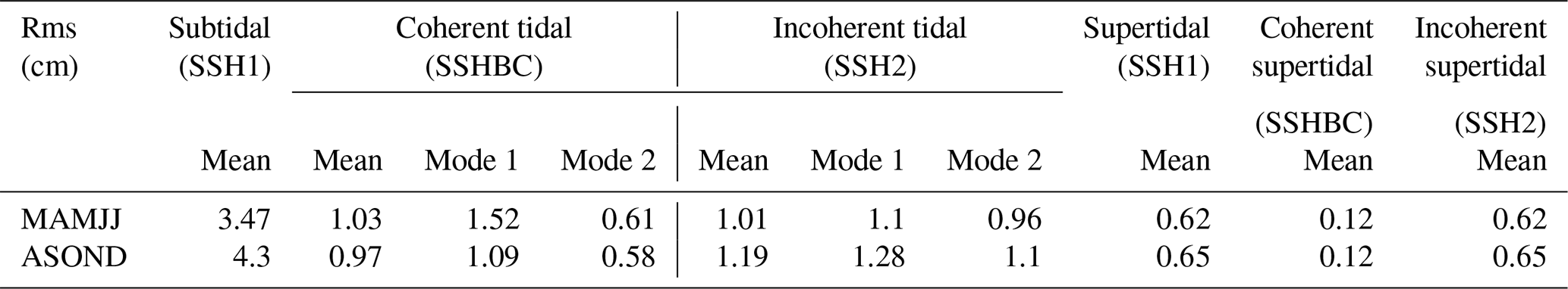
Table 2Rms of SSH1 at subtidal frequencies; coherent (SSHBC) and incoherent (SSH2) at tidal frequencies; and SSH1, SSHBC, and SSH2 at super tidal frequencies. Mean refers to the mean of rms in Figs. 10 and 11 over the model domain. Mode 1 and mode 2 refer to the rms deducted from the integration of spectra in Fig. 13 over the wavelength bands 150–100 and 100–70 km, respectively.
5.2 Meridional wavenumber spectrum and transition scale
In preparation for SWOT, it is important to know how the spatio-temporal SSH structures of the model depicted in Figs. 10 and 11 project onto frequency–wavenumber spectra and wavenumber spectra. Wavenumber spectra are often used to describe the spatial scales impacted by the ocean's turbulent energy cascade and to identify spatial scales impacted by the altimetric noise (Vergara et al., 2019; Xu and Fu, 2012; Chen and Qiu, 2021), or the spatial scales impacted by internal tides. Here, wavenumber spectra are evaluated in the 0–10∘ N, 43–45∘ W box where the rms of the subtidal, tidal, and supertidal SSHs are high (Fig. 10). The 10∘ latitudinal extension of the box limits the effects of overlap and flattening of the spectrum that would have occurred with a smaller latitudinal extension (Tchilibou et al., 2018).
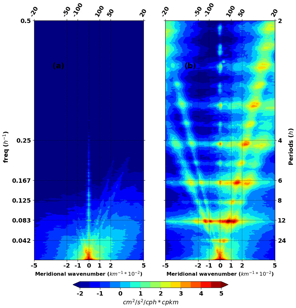
Figure 12Meridional frequency–wavenumber of (a) the hourly SSH of the model without tide (NTSSH) and (b) the hourly SSH1 of the model with tide, both during MAMJJ. SSH1 is the residual between hourly total SSH and the coherent barotropic SSH. Spectra are evaluated within 0–10∘ N, 43–45∘ W and averaged over the longitudes. Units: cm2 s−2 (cph cpkm)−1. Similar results are obtained for ASOND.
Examples of frequency–wavenumber spectra of hourly SSH1 (Fig. 12b) and of hourly SSH of the no-tide model (NTSSH, Fig. 12a) are shown in Fig. 12. The subtidal energy is unchanged between the two models while the SSH variances are at a maximum at diurnal (0.042 h−1, i.e. 12 h), semidiurnal (0.083 h−1, 12 h), and higher harmonic (8, 6, 4, 3 h) frequencies for the model with tide (Fig. 12b). The peaks at semidiurnal and diurnal frequencies are not isolated but linearly connected to each other. Such a high-frequency distribution of energy in the spectrum is linked to the IGW field (Farrar and Durland, 2012) that contributes to both tidal and supertidal variations (Fig. 12b). In Fig. 13, the SSH frequency–wavenumber spectra have been integrated over the different frequency bands to investigate the dominant spatial scales in terms of wavenumber spectra for the two seasons.
The altimetry data (Saral_full, black) and SSH1_full (blue) have both been corrected for the barotropic tide only. They show flatter SSH power spectrum density (PSD) spectral slopes over the 20–300 km wavelength range and are characterized by spectral peaks around 120 and 70 km. Despite the discrepancies at large scales and at scales smaller than 60 km, the agreement between altimetry and model reinforces our confidence in the model. At subtidal frequencies, the baroclinic SSH1_subtidal (red) is closer to SSH1_full (blue) from 1000 to 300 km in Fig. 13a and b. These SSH variances for scales larger than 300 km are mainly due to mesoscale and intraseasonal variability. From 300 to 30 km, the PSD spectrum for the model with no tides (NTSSH_subtidal; orange) and SSH1_subtidal (red) filtered spectrum both decrease sharply towards the smallest wavelengths (Fig. 13). In the classic “mesoscale” band from 250 to 70 km (delimited in Fig. 13 by the vertical dotted green line), the two spectra have slopes in K−4 and comparable rms values of 0.23 cm (SSH1_subtidal) and 0.21 cm (NTSSH_subtidal) during MAMJJ and 0.46 and 0.43 cm, respectively, during ASOND. So the observed increase in SSH PSD for scales between 250–70 km in altimeter data are dominated by tidal fluctuations (Fig. 13). In addition to presenting similar peaks at the same wavelengths, SSH1_full (blue) and SSH1_tidal (green) have similar rms values within the 250–70 km band: 2.46 and 2.4 cm, respectively, during MAMJJ and 2.57 and 2.43 cm, respectively, during ASOND. At wavelengths smaller than 60 km, the SSH1_full and SSH1_supertidal wavenumber spectra overlap during both MAMJJ and ASOND. These scales are dominated by IGW (Fig. 12).
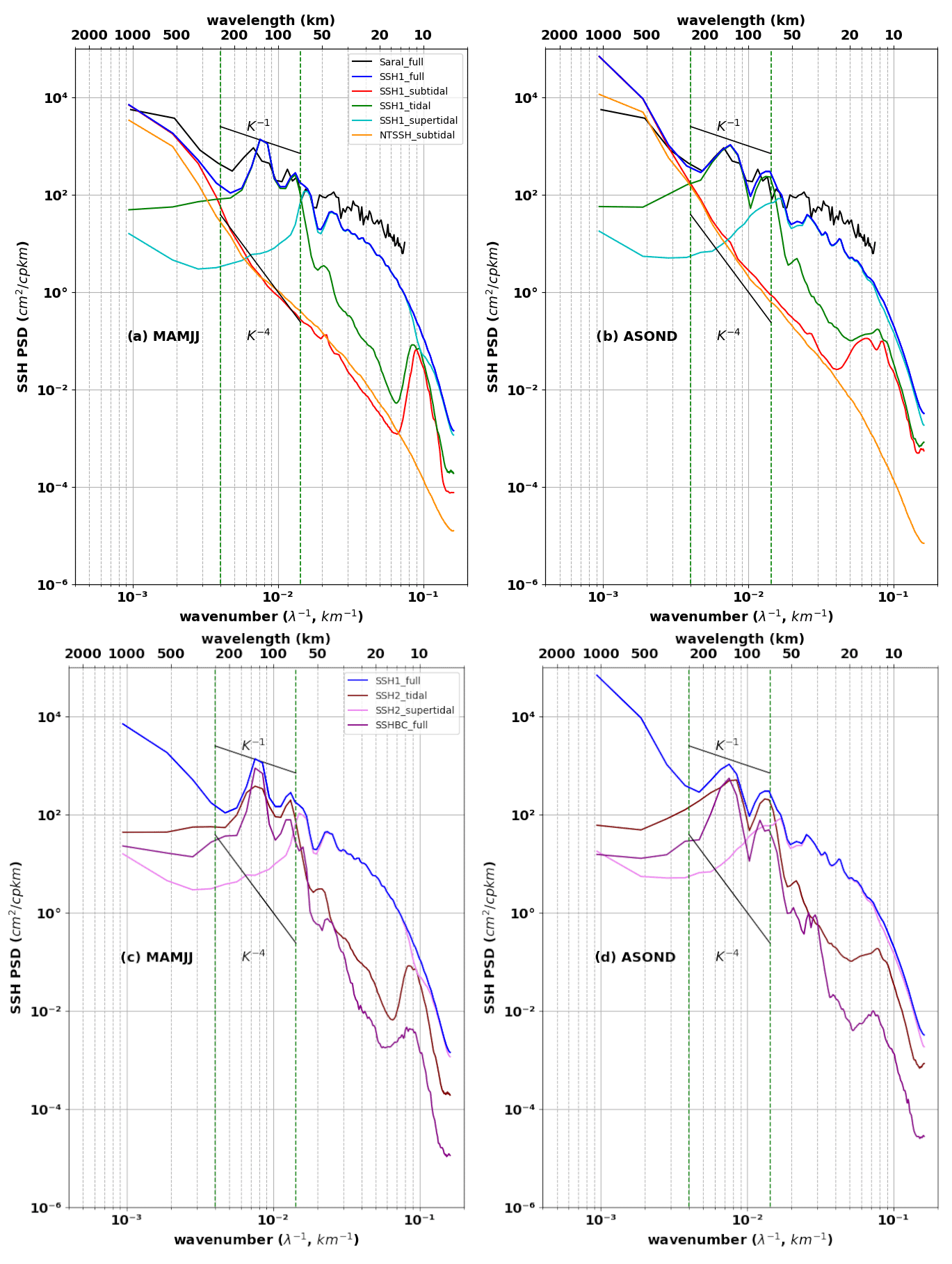
Figure 13SSH meridional wavenumber spectra separated into different frequency bands during (a, c) MAMJJ and (b, d) ASOND. (a, b) SSH1 (hourly residual between the total SSH and the coherent barotropic SSH, over all frequencies (full; blue), subtidal ( h−1); red), tidal ( h−1 f h−1; green) and supertidal frequencies ( h−1; cyan). Saral_full (in black) is the mean of SARAL/AltiKa along-track SSH spectra for the period 2013–2014, and NTSSH (orange) is the hourly SSH of the model with no tides. (c, d) Hourly coherent baroclinic SSH (SSHBC_full, purple) and SSH2 (hourly incoherent baroclinic SSH) at tidal (brown) and supertidal (pink) frequency bands. All spectra are evaluated within 0–10∘ N, 43–45∘ W and averaged over the longitudes. The vertical dotted green line delimits the classical 250–70 km mesoscale band. Units are in cm−2 cpkm−1.
The baroclinic contributions to the spectral PSD are shown in the lower panels of Fig. 13. The spectrum of the coherent internal tide's SSH (SSHBC_full, magenta) and the spectra of the incoherent SSH at tidal (SSH2_tidal, brown) and supertidal (SSH2_supertidal, pink) frequencies are presented in Fig. 13c and d. For the spectrum of SSHBC_full, there are clear peaks of mode 1 and mode 2 between 150–100 and 100–60 km. The peaks appear in the same ranges of wavelengths on the SSH2_subtidal spectrum (Fig. 13c and d). The SSH rms for mode 1 (within the wavelength band 150–100 km) and for mode 2 (within the wavelength band 100–60 km) are reported in Table 2. During the weak EKE period of MAMJJ, the rms of coherent SSH at tidal frequencies is 1.52 cm for mode 1 and 0.61 cm for mode 2, whereas the rms of the incoherent SSH is 1.1 and 0.96 cm, respectively (Table 2). They lead to 0.42 (mode 1) and 0.62 (mode 2) fraction of incoherence. So the SSH variances related to the incoherent component reach levels comparable to the coherent one for mode 1 and surpass it for mode 2. During the stronger EKE conditions in ASOND, the rms of coherent SSH at tidal frequency is 1.09 cm for mode 1 and 0.58 cm for mode 2. The rms of the incoherent modes is much larger during this period, 1.28 and 1.1 cm, respectively (Table 2), and the fraction of incoherence is 0.54 for mode 1 and 0.65 for mode 2. The incoherent SSH is thus more prominent at tidal frequencies during the strong EKE conditions of ASOND for mode 1 and mode 2.
Finally, it is relevant to know up to what wavelengths the geostrophic balance relation is still valid and to determine the wavelength of transition from which the mesoscale and sub-mesoscale dominate over non-geostrophic movements including the internal tide and the IGWs. The SSH1_subtidal spectrum associated with the mesoscale and sub-mesoscale first intersects the SSH1_tidal spectrum (dominated by the internal tide) around 250 km during MAMJJ and ASOND; it then intersects the SSH1_supertidal spectrum (dominated by the IGWs) at 166 km in MAMJJ and 142 km in ASOND (see Table 3). For both seasons, the spectra of SSH1_subtidal and SSH1_supertidal are such that the variance of SSH1 at tidal frequencies dominates the supertidal ones for scales above 60 km. It is therefore reasonable to set the transition scale at 250 km given the behaviour of the spectra of SSH1_subtidal and SSH1_tidal during the MAMJJ and ASOND seasons. This is similar to the transition scale in the Amazon region found by Qiu et al. (2018) based on a more complete dispersion relation analysis. This 250 km transition scale does not significant show seasonal variability from MAMJJ to ASOND (column 4 in Table 3). Indeed, the incoherent component is so important in the energetic ASOND that it shifts the transition scale by 50 km; it would have been 200 km using the coherent tidal SSH (Table 3). The tidal incoherence used to set the transition scale is dominated by the supertidal below 70 km (column 3 in Table 3). This confirms that the dynamics at scales below 60 km are governed by supertidal variations.
Table 3Transition length scale between balanced and unbalanced motion.
One of the challenges for the future SWOT mission is to propose appropriate processing to filter out most of the internal tide signals in the SSH products. Such an objective requires a clearer knowledge of internal tide dynamics including their temporal variability in various regions of the ocean. This study focuses on the Amazon shelf, one of the hotspots of M2 internal tide generation in the tropical Atlantic. The Amazon shelf is influenced by freshwater from river flow and precipitation below the ITCZ, as well as strong currents and eddies. The seasonal cycles of these oceanic, continental, and atmospheric forcings lead to two contrasting seasons (March to July – MAMJJ and August to December – ASOND) for which the properties of the M2 internal tide, the interaction of the internal tide with the circulation, and the SSH imprint of the internal tide have been explored. Barotropic and baroclinic tides were separated using vertical mode decomposition (Nugroho, 2017; Tchilibou et al., 2020). A harmonic analysis was performed in order to isolate the different components of the tide from which the coherent internal tide (phase-locked to barotropic tide) is deduced.
The analyses are based on 9.5 months (March to December 2015) of hourly outputs of a high-resolution (∘) NEMO numerical model forced by explicit tides. Model outputs are equally distributed between the two contrasted seasons MAMJJ and ASOND. During MAMJJ, the pycnocline is closer to the surface, slightly stronger, and quite horizontally homogeneous over the model domain. The currents and mesoscale activity are weak. During ASOND, the pycnocline is deeper (up to 50 m difference with MAMJJ), slightly weaker but with a strong horizontal gradient along the North Brazilian Current retroflexion and North Equatorial Countercurrent path. The currents and mesoscale activity became intense.
For both seasons, we have shown that the M2 barotropic tide originating from the southeastern open ocean is converted to M2 internal tide between the 100 m (the shelf break reference) and the 1000 m isobaths, with the maximum conversion occurring 10 km from the shelf break. The generated M2 internal tide then propagates mainly offshore in a northeasterly direction from sites A and B as in Magalhaes et al. (2016), but also from sites C, D, E, and F (see Fig. 1 for location). During ASOND, the M2 baroclinic fluxes are arrested around 6∘ N, especially east of 47∘ W. This behaviour of the baroclinic flux is different from that during MAMJJ and was first associated with an increase in dissipation. A proxy of the dissipation of the coherent baroclinic M2 was evaluated from the divergence of the M2 baroclinic flux and the M2 conversion rate. It is characterized by beam-like structures separated by 90 to 120 km. A distinction has been made between the local dissipation on the shelf break and the remote dissipation that occurs beyond 50 km from the shelf break. The local dissipation rate of the coherent baroclinic M2 increased from 17 % during ASOND to 23 % during MAMJJ because of strong higher-mode generation during MAMJJ. With the difference between the remote dissipation rates of the coherent baroclinic M2 not being significant, the hypothesis of a drastic increase in the dissipation was discarded. A temporal filter was then used to access the 25 h mean of the baroclinic flux, the relative vorticity, and the current. The filter allowed us to observe baroclinic flux variations over short periods and to get an idea of the interactions between the internal tide and the background circulation. The baroclinic fluxes coming from sites E and D undergo branching and merge with the baroclinic flux coming from neighbouring sites. The propagation of the baroclinic flux from F is a function of the intensity of the circulation, and it is well observed in periods of weak current and spring tides. The change of seasons between MAMJJ and ASOND is marked by an intensification of the circulation, which participates in deflecting the baroclinic flux from A further eastwards. It is therefore the changes in the interactions between internal tide and circulation, modulated by neap tide–spring tide cycles that explain the differences in baroclinic fluxes. The harmonic analysis at frequency M2 retained only the most relevant trajectories over the two periods.
The SSH has been separated into its coherent (phase-locked to barotropic forcing) and incoherent (with variable amplitude and phase) components. For each of the MAMJJ and ASOND seasons, the frequency and frequency–wavenumber spectra have been integrated for different frequency bands: the subtidal band for periods greater than 28 h counting for intraseasonal and mesoscale and sub-mesoscale variations, the tidal band between 28 and 11 h dominated by internal tide motions, and the supertidal band for periods less than 11 h where the inertial gravity waves are prominent. On the wavenumber spectra, it appears that the SSH variability for scales larger than 300 km is due to the intraseasonal and mesoscale and sub-mesoscale variability. Between 250 and 60 km, the SSH wavenumber spectra are flattened with peaks at mode 1 (150–100 km) and mode 2 (100–60 km) wavelength bands, and the SSH variance is related to the internal tide of tidal frequency. The supertidal and thus inertial gravity waves dominate scales under 60 km. At tidal and supertidal frequencies, the incoherent SSH induces SSH variations are of an order equal to or even greater than the coherent SSH. In the mode 1 wavelength band, the incoherent fraction (measuring how incoherent SSH is) is 0.4 during MAMJJ and 0.6 during ASOND. For mode 2 and wavelengths under 60 km, the incoherence fraction is higher than 0.5, marking a predominance of the incoherent tide. The transition scale corresponding to the wavelength at which the balanced (geostrophic) motion becomes more important than the unbalanced (non-geostrophic) motion was defined as the crossing wavelength of the SSH wavenumber spectra for subtidal and tidal frequencies. The transition scale is 250 km during MAMJJ for both coherent and incoherent SSHs at tidal frequencies. During ASOND, the transition scale is shifted from 200 km with the coherent to 250 km with the incoherent SSH. Even if coherent internal tide corrections are made available for conventional altimetry and SWOT data in this region, incoherent tides will still be present out to the transition scale wavelength of 250 km and will pollute the calculation of geostrophic currents at smaller scales.
Although this study provides some answers on the dynamics of the internal tide in this region of the tropical Atlantic, it raises other questions. The impression of non-propagation of the baroclinic tidal fluxes from sites E and D on the shelf break is, in our opinion, linked to the merging of these baroclinic fluxes with others. The branching of the baroclinic flux is probably an effect of refraction. However, the refraction here can be related to the density gradient at the front of the NBC retroflection or to the internal tidal interaction with the circulation (current and eddies). Much remains to be done to clearly describe the interaction of the internal tide with the background circulation in this area. An eastern extension of the model is being developed to distinguish whether the eastward deviation of the baroclinic flux from A is related to advection by the current or to strong refraction. With this new simulation, we hope to look at what happens to the baroclinic fluxes coming from C and B. It also remains to quantitatively determine the conditions under which the current advects the internal tide. According to Duda et al. (2018) as well as Kelly and Lermusiaux (2016), the angle between the mean current and the internal tide plays a role. The angle between the current and the baroclinic flux changes between 4–6∘ N in the eastern part of the basin during the passage from MAMJJ to ASOND, but it is premature to consider it as the essential element that imposes the trajectory of the baroclinic flux. Our study suggests that under real ocean conditions, the interaction between the internal tide and the current depends on the neap–spring cycle and the current intensity. All these parameters should be taken into account to define the significance threshold of the interaction between the internal tide and the current.
Intense semidiurnal internal solitary waves (ISWs, up to hundreds of kilometres from the shelf break) are consistently observed with SAR images propagating toward the open ocean in the Amazon area (Magalhaes et al., 2016; Jackson, 2004). These ISWs are associated with the instability and energy loss of internal tides coming from A and B (Magalhaes et al., 2016; Ivanov et al., 1990). Modulation of their propagation direction has been reported in Magalhaes et al. (2016), with the azimuth being larger in July–December (45∘) than in February–May (30∘). The authors suggest that the stronger NECC in July–December might be a likely explanation for the ISW seasonal deviation. In our opinion, the seasonal variability of the ISWs is not just related to the NECC but also to the variability of the interaction between internal tide and the background circulation, including all the diversity of the currents according to the vertical and the horizontal space, the eddies, and the stratification.
At the sites of internal tide generation, changes in stratification from MAMJJ to ASOND had an impact on the generation of higher modes, which is not surprising given that higher modes are best projected on density profiles with a stratification maximum near the ocean surface. Stratification has certainly played a role in the dissipation and propagation of the internal tide. In fact, the hotspots of M2 dissipation have been observed along propagating beams distant from about 90 to 120 km, in good agreement with previous simulations (Buijsman et al., 2016). The distance of 90 km smaller than a mode 1 baroclinic wavelength (120 km) suggests that the dissipation would occur in the water column between 100 and 500 m, depending on the thickness of the pycnocline. The vertically integrated dissipation proxy does not allow us to verify this. An analysis of the total dissipation similar to the work of Nugroho et al. (2018) would be appropriate. The 90 km distance could express a change of the mode 1 wavelength because of a change in stratification and in particular the depth of the pycnocline as discussed by Barbot et al. (2021). This is possible if the effects of stratification on the trajectory of the internal tide are stronger than those of the circulation (current and eddies). A quantitative study of the interactions between internal tide and the background circulation (stratification, currents, eddies) is essential.
The energy level of the SSH wavenumber spectra at subtidal frequencies is not exactly the same in the models with and without tide, especially at large scales and slightly at small scales. This is not surprising since the interactions between internal waves and eddies can enhance the forward energy cascade (Barkan et al., 2021; Thomas and Daniel, 2021) or stimulate the generation of sub-mesoscale ocean structures (Jensen et al., 2018). The analysis of SSH spectra deserves to be extended to energy in order to verify what happens to the energy transfer regime in this region. The transition scale we found may seem very large because we did not use any specific criterion to distinguish geostrophic from non-geostrophic motions outside of the temporal filter. We would have found a smaller transition scale varying by 24 km between MAMJJ and ASOND (see column 2 in Table 3), by applying the criteria of Savage et al. (2017) based on the ratio between the subtidal and supertidal spectra. Our approach with the temporal filter gives similar results to Qiu et al. (2018), who estimate the separation of geostrophic and non-geostrophic dynamics based on the vertical-mode IGW dispersion curve, although their calculation is not applied in the tropical band. The simpler filtering technique could be a starting point to determine the transition scale in other tropical regions. We note that the predicted standard deviations of the uncorrelated measurement error for the SWOT observations are 2.74 cm for the raw data on 1 km × 1 km grids and 1.35 cm in the case of 2 km × 2 km (Chelton et al., 2019): these noise levels are comparable to the SSH rms at supertidal to tidal frequencies. Our model results suggest that some high-frequency physical signals will be hidden by the SWOT noise in this Amazon region. The wavenumber frequency and the coherent baroclinic flux also highlight southward propagation of internal tide. It is possible that those entering the model area through its northern boundary originated from the Mid-Atlantic Ridge. Some of the wavenumber spectra are characterized by a hump at scales smaller than 20 km. We did not pay particular attention to this hump at 20 km, which is close to the model effective resolutions.
In the past decade, many investigations have been motivated by the internal tide surface signature corrections for all altimetry missions but especially for the future wide-swath altimetry SWOT mission. Various empirical atlases for surface internal tides have been derived from nearly 30 years of multi-mission altimetry, which reveal the coherent part of this signal over the altimetry era. The altimetry community's more pressing issue is the non-coherent part that is left aside in these atlases, whose magnitude and variability are the main concerns today as they will significantly contribute to the conventional altimetry and SWOT error budgets. Our investigations are a contribution to their quantification in a specific area and demonstrate the large variability of the internal tide dynamics at seasonal timescales. They also suggest even higher variability when considering shorter timescales because of the interaction with the upper ocean circulation, indicating clearly that the internal tide correction will be one of the most challenging problems for future altimetry data processing. In tropical regions with high seasonal variability, it is possible that internal tidal predictions at seasonal frequencies are more effective for altimetry data correction than annual prediction maps as currently proposed.
For more detailed investigations, we divide the shelf break into eight boxes of the same size as reported in Table A1 and plotted in Fig. 7a. Our modelled hotspots of internal tide generations are located at A (Aa + Ab) and B sites (in good agreement with Magalhaes et al., 2016). They respectively produce between 1.5 and 1.6 GW for A (Aa + Ab) and between 0.57 and 0.6 GW for B, depending on the season (MAMJJ or ASOND, Table A2).
Table A1Location of boxes surrounding internal tide generation hotspots. In brackets, the colour of the box is as in Fig. 7.

Table A2Energy balance in the different boxes, units: GW. divh(Fbt), Dbt, CVR, divh(Fbc), and Dbc are integrated in the boxes. We masked on the shelf where bathymetry is less than 100 m. P1 and P2 are defined by Eqs. (A1) and (A2), respectively.
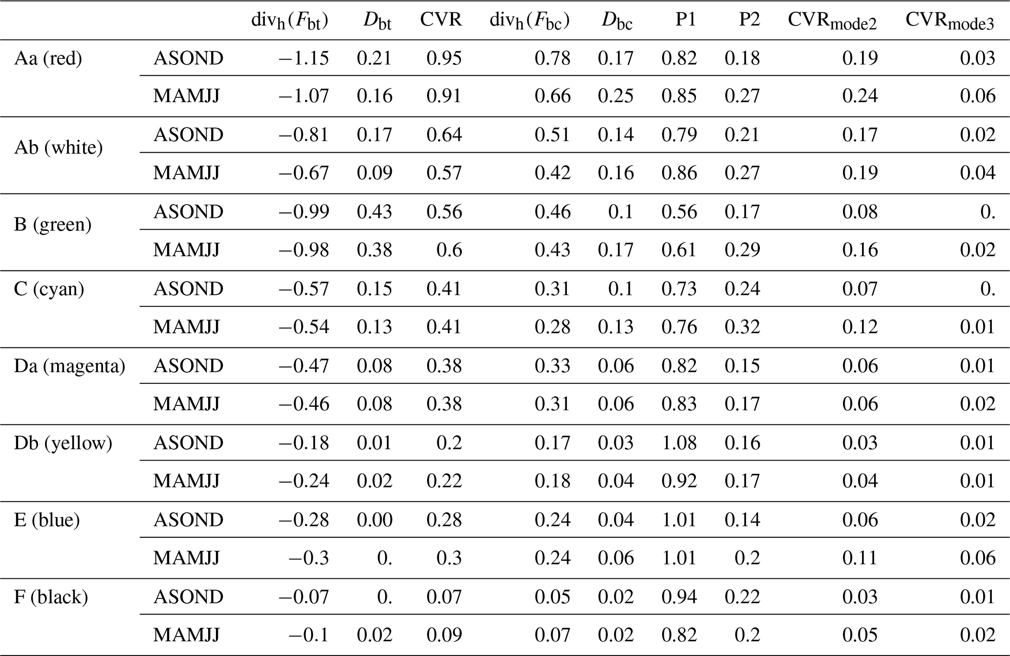
Sites C and Da also produce strong energy for internal tides (almost 0.4 GW, Table A2), whereas the other sites show lower baroclinic conversion rates with about 0.3 GW for E, 0.2 GW for Db, and 0.1 GW for F (Table A2). In Table A2, we also calculate the ratio P1 (Eq. A1), which can be seen as a proxy of the efficiency to convert internal tides from the barotropic flux.
For P1 close to 1, the internal tide generation explains most of the barotropic energy loss. If P1 is close to 0, then the divergence of the barotropic flux (divh(Fbt)) will be greater than the baroclinic conversion rate, meaning that the barotropic flux exports most of the barotropic energy out of the box without local generation of internal tides. In the case of the A site, almost 80 % of divh(Fbt) is converted into internal tides, with only 20 % flowing out of the shelf break in the Aa and Ab boxes. C and Da show similar behaviour to A. In contrast, the B site has a smaller P1 ratio of 60 %, and less energy is converted into internal tides. Actually, B has the same divh(Fbt) as A, but the efficiency to create internal tides is smaller (only 60 %). This is due to the fact that the barotropic flux (Fig. 6a and b) is perpendicular to the shelf break at the other sites (A, D, C, E, and F), which is more efficient to create propagating internal tides, whereas the angle is smaller in the case of B. For Db and F sites, the P1 ratio is even larger and close to 1. In this region north to 2∘ N (Db and F sites), the angle between the barotropic tides and the gradient of the topography is close to 90∘, which is the most efficient angle for conversion of barotropic to baroclinic tides (P1 close to 1). During the lower-energy MAMJJ season, the conversion rate CVR in A (Aa + Ab) is slightly smaller (−7 %) than in the more energetic ASOND (MAMJJ: 0.91 + 0.57 = 1.48 vs. ASOND: 0.95 + 0.64 = 1.59 GW, Table A2), whereas for B, Db, E, and F, it is the opposite (between 5 % and 10 % higher in MAMJJ than ASOND, Table A2). For C and Da the conversion rate remains identical between ASOND and MAMJJ. As shown in Table A2, the conversion efficiency (P1, Eq. A1) is higher in MAMJJ than in ASOND for the sites A to Da south of 2∘ N. It is the reverse (or unchanged) for the northern sites Db to F. These changes might be due to the stratification changes occurring from MAMJJ to ASOND and also between north and south of 2∘ N. The higher efficiency to convert to internal tides south of 2∘ N in MAMJJ compared to ASOND is associated with the shallower and stronger stratification (Fig. 5). The larger numbers (P1>1) found for E and Db sites may be due to some truncation errors.
At the generation sites, the conversion of internal tides (CVR column, Table A2) is balanced by the export further away through the baroclinic flux (divh(Fbc) column, Table A2) and the local dissipation (Dbc column, Table A2), following Eq. (2). In regions further away from generation sites, where CVR equals zero, the dissipation explains all the loss of baroclinic energy. Table A2 shows that dissipation is the highest for boxes A, B, and C (between 0.1 and 0.3 GW), with the highest value for Aa. Smaller values of the dissipation are obtained at D, E, and F (between 0.02 and 0.06 GW). Regarding divh(Fbc), the largest values are for Aa (between 0.6 and 0.8 GW) while Ab and B have relatively smaller values (between 0.4 and 0.5 GW). The divergence of the baroclinic flux gets smaller further northward (about 0.3 to 0.2 GW for C, Da, Db, and E) and is almost null for F. This is coherent with the baroclinic flux intensity (Fig. 7e and f), where the flux exported toward the open ocean is decreasing from A to F.
To discuss the dissipation, we defined the P2 ratio as follows:
P2 close to 1 means that internal tides generated in a box are dissipated locally there. In contrast, if P2 is close to 0, the energy of the baroclinic tides propagates out of the box. As an example for site Aa (Table A2), during ASOND, CVR = 0.95 GW and divh(Fbc)=0.78 GW are exported away while 0.17 GW dissipates locally, yielding P2 = 0.18, so 18 % of the internal tide energy generated in the box is locally dissipated. In fact, for the majority of the boxes, this ratio is between 15 % and 30 %, implying that 70 % to 85 % of baroclinic tide energy is radiated away. The largest P2 ratio occurs at C for both ASOND and MAMJJ (24 % and 32 %, respectively), then Aa (18 % and 29 %), Ab (21 % and 27 %), B (17 % and 29 %), F (22 % and 20 %), E (14 % and 22 %), and Da (15 % and 17 %) and Db (16 % and 17 %). For all sites except F, the P2 ratio is stronger in MAMJJ than ASOND, meaning that MAMJJ is more favourable to local dissipation. In the eight boxes, the generation of modes 2 and 3 is larger in MAMJJ compared to ASOND (see CVR for modes 2 and 3 columns of Table A2), as expected for a season with shallower pycnocline (Barbot et al., 2021). Once higher modes are generated, instabilities are more probable, and thus local dissipation is higher.
Data are available upon request by contacting the corresponding authors.
The supplement related to this article is available online at: https://doi.org/10.5194/os-18-1591-2022-supplement.
This work is part of the MT postdoc supervised by FL and AKL. JJ performed the numerical simulations, and MT made the analysis. The Argo data were pre-processed by SB. MT wrote the paper with contributions from all co-authors.
The contact author has declared that none of the authors has any competing interests.
Publisher's note: Copernicus Publications remains neutral with regard to jurisdictional claims in published maps and institutional affiliations.
We thank Damien Allain for helpful discussions. This work is a contribution to the project “Amazomix”.
Michel Tchilibou's postdoc is funded by CNRS. Ariane Koch Larrouy, Yves Morel, and Julien Jouanno are funded by IRD. Rosemary Morrow is funded by CNAP. Florent Lyard is funded by CNRS. Simon Barbot is funded by CNES (grant no. 2884), CLS, CNRS (grant no. 167349), and UPS.
This paper was edited by Neil Wells and reviewed by two anonymous referees.
Aguedjou, H. M. A., Dadou, I., Chaigneau, A., Morel, Y., and Alory, G.: Eddies in the Tropical Atlantic Ocean and Their Seasonal Variability, Geophys. Res. Lett., 46, 12156–12164, https://doi.org/10.1029/2019GL083925, 2019. a, b
Arbic, B., Richman, J., Shriver, J., Timko, P., Metzger, J., and Wallcraft, A.: Global Modeling of Internal Tides Within an Eddying Ocean General Circulation Model, Oceanography, 25, 20–29, https://doi.org/10.5670/oceanog.2012.38, 2012. a
Arbic, B. K., Wallcraft, A. J., and Metzger, E. J.: Concurrent simulation of the eddying general circulation and tides in a global ocean model, Ocean Model., 32, 175–187, https://doi.org/10.1016/j.ocemod.2010.01.007, 2010. a
Arbic, B. K., Alford, M. H., Ansong, J. K., Buijsman, M. C., Ciotti, R. B., Farrar, J. T., Hallberg, R. W., Henze, C. E., Hill, C. N., Luecke, C. A., Menemenlis, D., Metzger, E. J., Müeller, M., Nelson, A. D., Nelson, B. C., Ngodock, H. E., Ponte, R. M., Richman, J. G., Savage, A. C., Scott, R. B., Shriver, J. F., Simmons, H. L., Souopgui, I., Timko, P. G., Wallcraft, A. J., Zamudio, L., and Zhao, Z.: A Primer on Global Internal Tide and Internal Gravity Wave Continuum Modeling in HYCOM and MITgcm, in: New Frontiers in Operational Oceanography, edited by Chassignet, E. P., Pascual, A., Tintoré, J., and Verron, J.: GODAE OceanView, DigiNole, https://doi.org/10.17125/gov2018.ch13, 2018. a
Armi, L.: Effects of variations in eddy diffusivity on property distributions in the oceans, Woods Hole Oceanographic Institution, Woods Hole, MA, WHOAS, https://doi.org/10.1575/1912/10336, 1979. a
Baines, P.: On internal tide generation models, Deep-Sea Res. Pt. A, 29, 307–338, https://doi.org/10.1016/0198-0149(82)90098-X, 1982. a
Barbot, S., Lyard, F., Tchilibou, M., and Carrere, L.: Background stratification impacts on internal tide generation and abyssal propagation in the western equatorial Atlantic and the Bay of Biscay, Ocean Sci., 17, 1563–1583, https://doi.org/10.5194/os-17-1563-2021, 2021. a, b, c, d, e, f, g, h
Barkan, R., Srinivasan, K., Yang, L., McWilliams, J. C., Gula, J., and Vic, C.: Oceanic Mesoscale Eddy Depletion Catalyzed by Internal Waves, Geophys. Res. Lett., 48, e2021GL094376, https://doi.org/10.1029/2021GL094376, 2021. a
Barnier, B., Reynaud, T., Beckmann, A., Böning, C., Molines, J.-M., Barnard, S., and Jia, Y.: On the seasonal variability and eddies in the North Brazil Current: insights from model intercomparison experiments, Prog. Oceanogr., 48, 195–230, https://doi.org/10.1016/S0079-6611(01)00005-2, 2001. a
Beardsley, R. C., Candela, J., Limeburner, R., Geyer, W. R., Lentz, S. J., Castro, B. M., Cacchione, D., and Carneiro, N.: The M 2 tide on the Amazon Shelf, J. Geophys. Res., 100, 2283, https://doi.org/10.1029/94JC01688, 1995. a
Blayo, E. and Debreu, L.: Adaptive Mesh Refinement for Finite-Difference Ocean Models: First Experiments, J. Phys. Oceanogr., 29, 1239–1250, https://doi.org/10.1175/1520-0485(1999)029<1239:AMRFFD>2.0.CO;2, 1999. a
Buijsman, M. C., Ansong, J. K., Arbic, B. K., Richman, J. G., Shriver, J. F., Timko, P. G., Wallcraft, A. J., Whalen, C. B., and Zhao, Z.: Impact of Parameterized Internal Wave Drag on the Semidiurnal Energy Balance in a Global Ocean Circulation Model, J. Phys. Oceanogr., 46, 1399–1419, https://doi.org/10.1175/JPO-D-15-0074.1, 2016. a
Buijsman, M. C., Arbic, B. K., Richman, J. G., Shriver, J. F., Wallcraft, A. J., and Zamudio, L.: Semidiurnal internal tide incoherence in the equatorial Pacific, J. Geophys. Res.-Oceans, 122, 5286–5305, https://doi.org/10.1002/2016JC012590, 2017. a, b
Buijsman, M. C., Stephenson, G. R., Ansong, J. K., Arbic, B. K., Green, J. M., Richman, J. G., Shriver, J. F., Vic, C., Wallcraft, A. J., and Zhao, Z.: On the interplay between horizontal resolution and wave drag and their effect on tidal baroclinic mode waves in realistic global ocean simulations, Ocean Model., 152, 101656, https://doi.org/10.1016/j.ocemod.2020.101656, 2020. a
Carrère, L., Arbic, B. K., Dushaw, B., Egbert, G., Erofeeva, S., Lyard, F., Ray, R. D., Ubelmann, C., Zaron, E., Zhao, Z., Shriver, J. F., Buijsman, M. C., and Picot, N.: Accuracy assessment of global internal-tide models using satellite altimetry, Ocean Sci., 17, 147–180, https://doi.org/10.5194/os-17-147-2021, 2021. a
Carrère, L., Lyard, F., Cancet, M., Guillot, A., and Roblou, L.: FES 2012: A New Global Tidal Model Taking Advantage of Nearly 20 Years of Altimetry, Paper presented at the symposium 20 Years of Progress in Radar Altimetry, Venice, Italy, p. 6, 2012. a, b, c
Chelton, D. B., Schlax, M. G., Samelson, R. M., Farrar, J. T., Molemaker, M. J., McWilliams, J. C., and Gula, J.: Prospects for future satellite estimation of small-scale variability of ocean surface velocity and vorticity, Prog. Oceanogr., 173, 256–350, https://doi.org/10.1016/j.pocean.2018.10.012, 2019. a
Chen, S. and Qiu, B.: Sea Surface Height Variability in the 30–120 km Wavelength Band From Altimetry Along-Track Observations, J. Geophys. Res.-Oceans, 126, e2021JC017284, https://doi.org/10.1029/2021JC017284, 2021. a
de Lavergne, C., Madec, G., Le Sommer, J., Nurser, A. J. G., and Naveira Garabato, A. C.: The Impact of a Variable Mixing Efficiency on the Abyssal Overturning, J. Phys. Oceanogr., 46, 663–681, https://doi.org/10.1175/JPO-D-14-0259.1, 2016. a
Debreu, L.: Raffinement adaptatif de maillage et méthodes de zoom: application aux modèles d'océan, PhD thesis, thèse de doctorat dirigée par Le Dimet, François-Xavier et Blayo, Éric Mathématiques appliquées Grenoble, http://www.theses.fr/2000GRE10004 (last access: January 2022), 2000. a
Didden, N. and Schott, F.: Eddies in the North Brazil Current retroflection region observed by Geosat altimetry, J. Geophys. Res., 98, 20121, https://doi.org/10.1029/93JC01184, 1993. a
Duda, T. F., Lin, Y.-T., Buijsman, M., and Newhall, A. E.: Internal Tidal Modal Ray Refraction and Energy Ducting in Baroclinic Gulf Stream Currents, J. Phys. Oceanogr., 48, 1969–1993, https://doi.org/10.1175/JPO-D-18-0031.1, 2018. a, b
Dunphy, M. and Lamb, K. G.: Focusing and vertical mode scattering of the first mode internal tide by mesoscale eddy interaction: mode one focusing and scattering, J. Geophys. Res.-Oceans, 119, 523–536, https://doi.org/10.1002/2013JC009293, 2014. a
Dushaw, B. D., Worcester, P. F., and Dzieciuch, M. A.: On the predictability of mode-1 internal tides, Deep-Sea Res. Pt. I, 58, 677–698, https://doi.org/10.1016/j.dsr.2011.04.002, 2011. a
Dussin, R., Barnier, B., Brodeau, L., and Molines, J. M.: The Making of the DRAKKAR FORCING SET DFS5, p. 34, DRAKKAR/MyOcean Report 01-04-16, LGGE, Grenoble, France, 2016. a
Farrar, J. T. and Durland, T. S.: Wavenumber–Frequency Spectra of Inertia–Gravity and Mixed Rossby–Gravity Waves in the Equatorial Pacific Ocean, J. Phys. Oceanogr., 42, 1859–1881, https://doi.org/10.1175/JPO-D-11-0235.1, 2012. a
Ffield, A.: North Brazil current rings viewed by TRMM Microwave Imager SST and the influence of the Amazon Plume, Deep-Sea Res. Pt. I, 52, 137–160, https://doi.org/10.1016/j.dsr.2004.05.013, 2005. a
Fratantoni, D. M. and Glickson, D. A.: North Brazil Current Ring Generation and Evolution Observed with SeaWiFS, J. Phys. Oceanogr., 32, 1058–1074, https://doi.org/10.1175/1520-0485(2002)032<1058:NBCRGA>2.0.CO;2, 2002. a
Fu, L.-L. and Ferrari, R.: Observing Oceanic Submesoscale Processes From Space, EOS T. Am. Geophys. Un., 89, 488–488, https://doi.org/10.1029/2008EO480003, 2008. a
Fu, L.-L. and Ubelmann, C.: On the Transition from Profile Altimeter to Swath Altimeter for Observing Global Ocean Surface Topography, J. Atmos. Ocean. Tech., 31, 560–568, https://doi.org/10.1175/JTECH-D-13-00109.1, 2014. a
Fu, L.-L., Alsdorf, D., Rodriguez, E., Morrow, R., Mognard, N., Lambin, J., Vaze, P., and Lafon, T.: THE SURFACE WATER AND OCEAN TOPOGRAPHY (SWOT) MISSION, p. 9, 2009. a
Gabioux, M., Vinzon, S. B., and Paiva, A. M.: Tidal propagation over fluid mud layers on the Amazon shelf, Cont. Shelf Res., 25, 113–125, https://doi.org/10.1016/j.csr.2004.09.001, 2005. a
Garraffo, Z. D., Johns, W. E., Chassignet, E. P., and Goni, G. J.: North Brazil Current rings and transport of southern waters in a high resolution numerical simulation of the North Atlantic, in: Elsevier Oceanography Series, edited by: Goni, G. J. and Malanotte-Rizzoli, P., Vol. 68 of Interhemispheric Water Exchange in the Atlantic Ocean, 375–409, Elsevier, https://doi.org/10.1016/S0422-9894(03)80155-1, 2003. a
Garzoli, S. L.: North Brazil Current retroflection and transports, J. Geophys. Res., 109, C01013, https://doi.org/10.1029/2003JC001775, 2004. a
Gerkema, T.: Internal and interfacial tides: Beam scattering and local generation of solitary waves, J. Marine Res., 59, 227–255, https://doi.org/10.1357/002224001762882646, 2001. a, b
Gerkema, T.: Development of internal solitary waves in various thermocline regimes – a multi-modal approach, Nonlin. Processes Geophys., 10, 397–405, https://doi.org/10.5194/npg-10-397-2003, 2003. a, b
Gerkema, T., Lam, F. A., and Maas, L. R. M.: Internal tides in the Bay of Biscay: conversion rates and seasonal effects, Deep-Sea Res. Pt. II, 51, 2995–3008, https://doi.org/10.1016/j.dsr2.2004.09.012, 2004. a
Geyer, W. R.: Tide-induced mixing in the Amazon Frontal Zone, J. Geophys. Res., 100, 2341, https://doi.org/10.1029/94JC02543, 1995. a, b
Gill, A. E.: Atmosphere-ocean dynamics, no. 30 in International geophysics series, Acad. Press, San Diego, oCLC: 249294465, 2003. a
Gurvan, M., Bourdallé-Badie, R., Chanut, J., Clementi, E., Coward, A., Ethé, C., Iovino, D., Lea, D., Lévy, C., Lovato, T., Martin, N., Masson, S., Mocavero, S., Rousset, C., Storkey, D., Vancoppenolle, M., Müeller, S., Nurser, G., Bell, M., and Samson, G.: NEMO ocean engine, Zenodo [code], https://doi.org/10.5281/ZENODO.1464816, 2019. a
Ivanov, V. A., Ivanov, L. I., and Lisichenok, A. D.: Redistribution of energy of the internal tidal wave in the North Equatorial Countercurrent region, Soviet Journal of Physical Oceanography, 1, 383–386, https://doi.org/10.1007/BF02196837, 1990. a
Jackson, C. R.: An Atlas of Internal Solitary-like Waves and Their Properties, 2nd Edn., Global Ocean Associates, Alexandria, VA, 560 pp., http://www.internalwaveatlas.com (last access: January 2022), 2004. a
Jensen, T. G., Shulman, I., Wijesekera, H. W., Anderson, S., and Ladner, S.: Submesoscale features and their interaction with fronts and internal tides in a high-resolution coupled atmosphere-ocean-wave model of the Bay of Bengal, Ocean Dynam., 68, 391–410, https://doi.org/10.1007/s10236-018-1136-x, 2018. a
Johns, W. E., Lee, T. N., Beardsley, R. C., Candela, J., Limeburner, R., and Castro, B.: Annual Cycle and Variability of the North Brazil Current, p. 26, https://doi.org/10.1175/1520-0485(1998)028<0103:ACAVOT>2.0.CO;2, 1998. a, b
Kelly, S. M.: The Vertical Mode Decomposition of Surface and Internal Tides in the Presence of a Free Surface and Arbitrary Topography, J. Phys. Oceanogr., 46, 3777–3788, https://doi.org/10.1175/JPO-D-16-0131.1, 2016. a, b
Kelly, S. M. and Lermusiaux, P. F. J.: Internal-tide interactions with the Gulf Stream and Middle Atlantic Bight shelfbreak front: INTERNAL-TIDE INTERACTIONS, J. Geophys. Res.-Oceans, 121, 6271–6294, https://doi.org/10.1002/2016JC011639, 2016. a
Kelly, S. M., Nash, J. D., and Kunze, E.: Internal-tide energy over topography, J. Geophys. Res., 115, C06014, https://doi.org/10.1029/2009JC005618, 2010. a, b, c, d
Kelly, S. M., Lermusiaux, P. F. J., Duda, T. F., and Haley, P. J.: A Coupled-Mode Shallow-Water Model for Tidal Analysis: Internal Tide Reflection and Refraction by the Gulf Stream, J. Phys. Oceanogr., 46, 3661–3679, https://doi.org/10.1175/JPO-D-16-0018.1, 2016. a
Koch-Larrouy, A., Lengaigne, M., Terray, P., Madec, G., and Masson, S.: Tidal mixing in the Indonesian Seas and its effect on the tropical climate system, Clim. Dynam., 34, 891–904, https://doi.org/10.1007/s00382-009-0642-4, 2010. a
Kunze, E., Rosenfeld, L. K., Carter, G. S., and Gregg, M. C.: Internal Waves in Monterey Submarine Canyon, J. Phys. Oceanogr., 32, 1890–1913, https://doi.org/10.1175/1520-0485(2002)032<1890:IWIMSC>2.0.CO;2, 2002. a, b
Kurapov, A. L., Egbert, G. D., Allen, J. S., Miller, R. N., Erofeeva, S. Y., and Kosro, P. M.: The M2 Internal Tide off Oregon: Inferences from Data Assimilation, J. Phys. Oceanogr., 33, 1733–1757, https://doi.org/10.1175/2397.1, 2003. a
Lahaye, N., Gula, J., and Roullet, G.: Sea Surface Signature of Internal Tides, Geophys. Res. Lett., 46, 3880–3890, https://doi.org/10.1029/2018GL081848, 2019. a
Laurent, L. S. and Garrett, C.: The Role of Internal Tides in Mixing the Deep Ocean, J. Phys. Oceanogr., 32, 2882–2899, https://doi.org/10.1175/1520-0485(2002)032<2882:TROITI>2.0.CO;2, 2002. a
Le Bars, Y., Lyard, F., Jeandel, C., and Dardengo, L.: The AMANDES tidal model for the Amazon estuary and shelf, Ocean Model., 31, 132–149, https://doi.org/10.1016/j.ocemod.2009.11.001, 2010. a
Lentz, S. J.: Seasonal variations in the horizontal structure of the Amazon Plume inferred from historical hydrographic data, J. Geophys. Res., 100, 2391, https://doi.org/10.1029/94JC01847, 1995. a
Lentz, S. J. and Limeburner, R.: The Amazon River Plume during AMASSEDS: Spatial characteristics and salinity variability, J. Geophys. Res., 100, 2355, https://doi.org/10.1029/94JC01411, 1995. a, b
Li, Q., Mao, X., Huthnance, J., Cai, S., and Kelly, S.: On Internal Waves Propagating across a Geostrophic Front, J. Phys. Oceanogr., 49, 1229–1248, https://doi.org/10.1175/JPO-D-18-0056.1, 2019. a
Lyard, F. H., Allain, D. J., Cancet, M., Carrère, L., and Picot, N.: FES2014 global ocean tide atlas: design and performance, Ocean Sci., 17, 615–649, https://doi.org/10.5194/os-17-615-2021, 2021. a
Magalhaes, J. M., da Silva, J. C. B., Buijsman, M. C., and Garcia, C. A. E.: Effect of the North Equatorial Counter Current on the generation and propagation of internal solitary waves off the Amazon shelf (SAR observations), Ocean Sci., 12, 243–255, https://doi.org/10.5194/os-12-243-2016, 2016. a, b, c, d, e, f, g, h, i
Marin, F., Caniaux, G., Giordani, H., Bourlès, B., Gouriou, Y., and Key, E.: Why Were Sea Surface Temperatures so Different in the Eastern Equatorial Atlantic in June 2005 and 2006?, J. Phys. Oceanogr., 39, 1416–1431, https://doi.org/10.1175/2008JPO4030.1, 2009. a
Molleri, G. S., Novo, E. M. M., and Kampel, M.: Space-time variability of the Amazon River plume based on satellite ocean color, Cont. Shelf Res., 30, 342–352, https://doi.org/10.1016/j.csr.2009.11.015, 2010. a, b
Morrow, R., Fu, L.-L., Ardhuin, F., Benkiran, M., Chapron, B., Cosme, E., d’Ovidio, F., Farrar, J. T., Gille, S. T., Lapeyre, G., Le Traon, P.-Y., Pascual, A., Ponte, A., Qiu, B., Rascle, N., Ubelmann, C., Wang, J., and Zaron, E. D.: Global Observations of Fine-Scale Ocean Surface Topography With the Surface Water and Ocean Topography (SWOT) Mission, Front. Mar. Sci., 6, 232, https://doi.org/10.3389/fmars.2019.00232, 2019. a
Munk, W. and Wunsch, C.: Abyssal recipes II: energetics of tidal and wind mixing, Deep-Sea Res. Pt. I, 45, 1977–2010, https://doi.org/10.1016/S0967-0637(98)00070-3, 1998. a
Müller, M., Cherniawsky, J. Y., Foreman, M. G. G., and von Storch, J.-S.: Global M2 internal tide and its seasonal variability from high resolution ocean circulation and tide modeling: M2 INTERNAL TIDE, Geophys. Res. Lett., 39, L19607, https://doi.org/10.1029/2012GL053320, 2012. a
Müller, M., Cherniawsky, J. Y., Foreman, M. G. G., and von Storch, J.-S.: Seasonal variation of the M 2 tide, Ocean Dynam., 64, 159–177, https://doi.org/10.1007/s10236-013-0679-0, 2014. a
Nash, J., Shroyer, E., Kelly, S., Inall, M., Duda, T., Levine, M., Jones, N., and Musgrave, R.: Are Any Coastal Internal Tides Predictable?, Oceanography, 25, 80–95, https://doi.org/10.5670/oceanog.2012.44, 2012. a, b, c
Neto, A. V. N. and da Silva, A. C.: Seawater temperature changes associated with the North Brazil current dynamics, Ocean Dynam., 64, 13–27, https://doi.org/10.1007/s10236-013-0667-4, 2014. a, b
Niwa, Y. and Hibiya, T.: Estimation of baroclinic tide energy available for deep ocean mixing based on three-dimensional global numerical simulations, J. Oceanogr., 67, 493–502, https://doi.org/10.1007/s10872-011-0052-1, 2011. a
Niwa, Y. and Hibiya, T.: Generation of baroclinic tide energy in a global three-dimensional numerical model with different spatial grid resolutions, Ocean Model., 80, 59–73, https://doi.org/10.1016/j.ocemod.2014.05.003, 2014. a
Nugroho, D.: La marée dans un modèle de circulation générale dans les mers indonésiennes, PhD, Université de Toulouse, Université Toulouse III – Paul Sabatier, http://thesesups.ups-tlse.fr/3614/ (last access: January 2022), 2017. a, b, c
Nugroho, D., Koch-Larrouy, A., Gaspar, P., Lyard, F., Reffray, G., and Tranchant, B.: Modelling explicit tides in the Indonesian seas: An important process for surface sea water properties, Mar. Pollut. Bull., 131, 7–18, https://doi.org/10.1016/j.marpolbul.2017.06.033, 2018. a, b
Ponte, A. L. and Klein, P.: Incoherent signature of internal tides on sea level in idealized numerical simulations, Geophys. Res. Lett., 42, 1520–1526, https://doi.org/10.1002/2014GL062583, 2015. a
Qiu, B., Chen, S., Klein, P., Wang, J., Torres, H., Fu, L.-L., and Menemenlis, D.: Seasonality in Transition Scale from Balanced to Unbalanced Motions in the World Ocean, J. Phys. Oceanogr., 48, 591–605, https://doi.org/10.1175/JPO-D-17-0169.1, 2018. a, b, c
Rainville, L., Lee, C. M., Rudnick, D. L., and Yang, K.-C.: Propagation of internal tides generated near Luzon Strait: Observations from autonomous gliders, J. Geophys. Res.-Oceans, 118, 4125–4138, https://doi.org/10.1002/jgrc.20293, 2013. a
Ray, R. D. and Mitchum, G. T.: Surface manifestation of internal tides in the deep ocean: observations from altimetry and island gauges, Prog. Oceanogr., 40, 135–162, https://doi.org/10.1016/S0079-6611(97)00025-6, 1997. a
Ray, R. D. and Zaron, E. D.: Non-stationary internal tides observed with satellite altimetry, Geophys. Res. Lett., 38, L17609, https://doi.org/10.1029/2011GL048617, 2011. a
Ray, R. D. and Zaron, E. D.: M2 Internal Tides and Their Observed Wavenumber Spectra from Satellite Altimetry, J. Phys. Oceanogr., 46, 3–22, https://doi.org/10.1175/JPO-D-15-0065.1, 2016. a, b, c, d, e, f
Richardson, P. L., Hufford, G. E., Limeburner, R., and Brown, W. S.: North Brazil Current retroflection eddies, J. Geophys. Res., 99, 5081, https://doi.org/10.1029/93JC03486, 1994. a
Ruault, V., Jouanno, J., Durand, F., Chanut, J., and Benshila, R.: Role of the Tide on the Structure of the Amazon Plume: A Numerical Modeling Approach, J. Geophys. Res.-Oceans, 125, e2019JC015495, https://doi.org/10.1029/2019JC015495, 2020. a, b, c, d
Savage, A. C., Arbic, B. K., Richman, J. G., Shriver, J. F., Alford, M. H., Buijsman, M. C., Thomas Farrar, J., Sharma, H., Voet, G., Wallcraft, A. J., and Zamudio, L.: Frequency content of sea surface height variability from internal gravity waves to mesoscale eddies: FREQUENCY CONTENT OF SEA SURFACE HEIGHT, J. Geophys. Res.-Oceans, 122, 2519–2538, https://doi.org/10.1002/2016JC012331, 2017. a, b
Shriver, J. F., Arbic, B. K., Richman, J. G., Ray, R. D., Metzger, E. J., Wallcraft, A. J., and Timko, P. G.: An evaluation of the barotropic and internal tides in a high-resolution global ocean circulation model: Barotropic and Internal Tides in HYCOM, J. Geophys. Res.-Oceans, 117, C10024, https://doi.org/10.1029/2012JC008170, 2012. a
Shriver, J. F., Richman, J. G., and Arbic, B. K.: How stationary are the internal tides in a high-resolution global ocean circulation model?, J. Geophys. Res.-Oceans, 119, 2769–2787, https://doi.org/10.1002/2013JC009423, 2014. a
Silva, A., Araujo, M., Medeiros, C., Silva, M., and Bourles, B.: Seasonal changes in the mixed and barrier layers in the western Equatorial Atlantic, Braz. J. Oceanogr., 53, 83–98, https://doi.org/10.1590/S1679-87592005000200001, 2005. a, b
Silva, A. C., Bourles, B., and Araujo, M.: Circulation of the thermocline salinity maximum waters off the Northern Brazil as inferred from in situ measurements and numerical results, Ann. Geophys., 27, 1861–1873, https://doi.org/10.5194/angeo-27-1861-2009, 2009. a
So-Hybam: Observation Service SO HYBAM Geodynamical, hydrological and biogeochemical control of erosion/alteration and material transport in the Amazon, Orinoco and Congo basins, So-Hybam [data set], http://www.ore-hybam.org/ (last access: 2 September 2022), 2019. a
Soufflet, Y., Marchesiello, P., Lemarié, F., Jouanno, J., Capet, X., Debreu, L., and Benshila, R.: On effective resolution in ocean models, Ocean Model., 98, 36–50, https://doi.org/10.1016/j.ocemod.2015.12.004, 2016. a
Stammer, D., Ray, R. D., Andersen, O. B., Arbic, B. K., Bosch, W., Carrère, L., Cheng, Y., Chinn, D. S., Dushaw, B. D., Egbert, G. D., Erofeeva, S. Y., Fok, H. S., Green, J. A. M., Griffiths, S., King, M. A., Lapin, V., Lemoine, F. G., Luthcke, S. B., Lyard, F., Morison, J., Müller, M., Padman, L., Richman, J. G., Shriver, J. F., Shum, C. K., Taguchi, E., and Yi, Y.: Accuracy assessment of global barotropic ocean tide models, Rev. Geophys., 52, 243–282, https://doi.org/10.1002/2014RG000450, 2014. a
Szekely, T., Gourrion, J., Pouliquen, S., and Reverdin, G.: CORA, Coriolis Ocean Dataset for Reanalysis, SEANOE [data set], https://doi.org/10.17882/46219, 2019. a
Tchilibou, M., Gourdeau, L., Morrow, R., Serazin, G., Djath, B., and Lyard, F.: Spectral signatures of the tropical Pacific dynamics from model and altimetry: a focus on the meso-/submesoscale range, Ocean Sci., 14, 1283–1301, https://doi.org/10.5194/os-14-1283-2018, 2018. a
Tchilibou, M., Gourdeau, L., Lyard, F., Morrow, R., Koch Larrouy, A., Allain, D., and Djath, B.: Internal tides in the Solomon Sea in contrasted ENSO conditions, Ocean Sci., 16, 615–635, https://doi.org/10.5194/os-16-615-2020, 2020. a, b, c, d, e
Thomas, J. and Daniel, D.: Forward flux and enhanced dissipation of geostrophic balanced energy, J. Fluid Mech., 911, A60, https://doi.org/10.1017/jfm.2020.1026, 2021. a
Vergara, O., Morrow, R., Pujol, I., Dibarboure, G., and Ubelmann, C.: Revised Global Wave Number Spectra From Recent Altimeter Observations, J. Geophys. Res.-Oceans, 124, 3523–3537, https://doi.org/10.1029/2018JC014844, 2019. a
Verron, J., Sengenes, P., Lambin, J., Noubel, J., Steunou, N., Guillot, A., Picot, N., Coutin-Faye, S., Sharma, R., Gairola, R. M., Murthy, D. V. A. R., Richman, J. G., Griffin, D., Pascual, A., Rémy, F., and Gupta, P. K.: The SARAL/AltiKa Altimetry Satellite Mission, Mar. Geodesy, 38, 2–21, https://doi.org/10.1080/01490419.2014.1000471, 2015. a
Weatherall, P., Marks, K. M., Jakobsson, M., Schmitt, T., Tani, S., Arndt, J. E., Rovere, M., Chayes, D., Ferrini, V., and Wigley, R.: A new digital bathymetric model of the world's oceans, Earth Space Sci., 2, 331–345, https://doi.org/10.1002/2015EA000107, 2015. a
Xu, Y. and Fu, L.-L.: The Effects of Altimeter Instrument Noise on the Estimation of the Wavenumber Spectrum of Sea Surface Height, J. Phys. Oceanogr., 42, 2229–2233, https://doi.org/10.1175/JPO-D-12-0106.1, 2012. a
Zaron, E. D. and Egbert, G. D.: Time-Variable Refraction of the Internal Tide at the Hawaiian Ridge, J. Phys. Oceanogr., 44, 538–557, https://doi.org/10.1175/JPO-D-12-0238.1, 2014. a
Zhao, Z., Alford, M. H., Girton, J. B., Rainville, L., and Simmons, H. L.: Global Observations of Open-Ocean Mode-1 M2 Internal Tides, J. Phys. Oceanogr., 46, 1657–1684, https://doi.org/10.1175/JPO-D-15-0105.1, 2016. a, b, c
Zilberman, N. V., Merrifield, M. A., Carter, G. S., Luther, D. S., Levine, M. D., and Boyd, T. J.: Incoherent Nature of M2 Internal Tides at the Hawaiian Ridge, J. Phys. Oceanogr., 41, 2021–2036, https://doi.org/10.1175/JPO-D-10-05009.1, 2011. a, b
- Abstract
- Introduction
- Data and method
- Model validation and contrasting season
- Internal tide characteristics
- Coherent and incoherent SSH for MAMJJ and ASOND
- Summary
- Discussions and perspectives
- Appendix A
- Data availability
- Author contributions
- Competing interests
- Disclaimer
- Acknowledgements
- Financial support
- Review statement
- References
- Supplement