A numerical study of near-inertial motions in the Mid-Atlantic Bight area induced by Hurricane Irene (2011)

Hurricane Irene generated strong near-inertial currents (NICs) in ocean waters when passing over the Mid-Atlantic Bight (MAB) of the US East Coast in late August 2011. It is demonstrated that a combination of valuable field data and detailed model results can be taken advantage of to study the development and decay mechanism of this event. Numerical results obtained with the Regional Oceanic Modeling System (ROMS) are shown to agree well with the field data. Both computed and observed results show that the NICs were significant in most areas of the MAB region except in the nearshore area where the stratification was totally destroyed by the hurricane-induced strong mixing. Based on the energy budget, it is clarified that the near-inertial kinetic energy (NIKE) was mainly gained from the wind power during the hurricane event. In the deepwater region, NIKE was basically balanced by the vertical turbulence diffusion (40 %) and downward divergence (33 %), while in the continental shelf region, NIKE was mainly dissipated by the vertical turbulence diffusion (67 %) and partially by the bottom friction (24 %). Local dissipation of NIKE due to turbulence diffusion is much more closely related to the rate of the vertical shear rather than the intensity of turbulence. The strong vertical shear at the offshore side of the continental shelf led to a rapid dissipation of NIKE in this region.

1 Introduction

Near-inertial currents (NICs), which are widely observed in ocean basins around the world, are characterized by the important role of the Coriolis effect and by periodic motion with the frequency of an inertial mode (Garrett, 2001). The basic energy source of these freely flowing currents is wind power (Pollard, 1980; D'Asaro et al., 1985). Globally, the annually averaged wind power supply to NICs was estimated to range from 0.3 TW to more than 1 TW by previous investigators (Alford, 2003a; Furuichi et al., 2008; Rimac et al., 2013). As a comparison, the total power required to maintain abyssal stratification and thermohaline circulation is about 2 TW (Munk and Wunsch, 1998). This implies that the NIC is a very important phenomenon in physical oceanography (Gregg, 1987; Alford, 2003b; Jochum et al., 2013).

A tropical or extratropical cyclone (hereinafter collectively referred to as TC) is a rotating low-pressure and strong-wind mesoscale weather system, which generates NICs more powerfully than other types of atmospheric processes in nature (Alford et al., 2016; Steiner et al., 2017). When a TC passes over a deep ocean, enormous energy is directly transferred into the ocean waters, which rapidly generates strong NICs with a velocity up to 1 m s⁻¹ in the horizontal direction of the mixed layer (Price, 1983; Sanford et al., 2011). A right-bias effect is often shown in the NIC pattern, i.e., NICs are more intense on the right side of the hurricane track, due to the resonance between the surface flow driven by NICs and clockwise-rotating wind stress on the right side (Chang and Anthes, 1978; Price et al., 1994). After the passage of a TC, the surface near-inertial energy usually persists for several inertial cycles and then gradually decays (Price, 1983; Sanford et al., 2011; Hormann et al., 2014; Zhang et al., 2016; Wu et al., 2020).

It is known that NICs in shallow waters show some significant differences with those in deep waters, and the velocity of NICs in shallow waters is usually of a smaller magnitude of 0.1–0.5 m s⁻¹ (Chen and Xie, 1997; Rayson et al., 2015; Yang et al., 2015; Chen et al., 2017; Zhang et al., 2018). The decrease i current velocity in shallow waters may be an effect of the sea-bottom friction as Rayson et al. (2015) pointed out. Chen and Xie (1997), however, found that it was because a significant part of the wind input, which may otherwise be an energy source of the NICs, was exhausted to generate a wave-induced nearshore current system. Chen et al. (2017) considered that barotropic waves in shallow waters, such as seiches, may trap some wind energy. In addition to the difference in magnitude, the modes of the NICs in shallow and deep waters are also different. More specifically, a two-layer structure was observed in shallow waters in several studies, i.e., NICs were in opposite phases in surface and bottom layers, which differed from the conventional multi-layer mode in deep waters (Chen et al., 1996; Shearman, 2005; Yang et al., 2015), though a multi-layer mode may also sometimes be observed in nearshore waters due to the combined effect of changing wind stress, variable stratification, and nonlinear bottom friction (MacKinnon and Gregg, 2005).

There have been a considerable number of studies on the decay of specific TC-generated NICs in coastal regions. Rayson et al. (2015) paid attention to four intense TCs on the Australian North West Shelf and related the rapid decay of NICs in shallow waters to the bottom friction. Yang et al. (2015) examined coastal ocean responses to Typhoon Washi and found that the negative background vorticity could trap near-inertial energy and result in a slow decay. Shen et al. (2017) investigated five TCs over the Taiwan Strait and identified a rapid decaying rate due to nonlinear interaction between NICs and tides. Zhang et al. (2018) studied Hurricane Arthur in the Mid-Atlantic Bight and showed that excessive wind input does not necessarily lead to amplification of NICs because intensive wind input is usually accompanied by an even higher rate of energy dissipation.

Though a significant number of investigations have been conducted, some basic features of a TC-induced NIC in the coastal ocean are still not clarified. For instance, the energy budget in the NIC generated by a TC has not yet been thoroughly discussed in either deep or shallow waters, and the relative importance of different physical processes, including advection, conversion, turbulence diffusion, bottom friction, and energy divergence, in the energy budget has not yet been fully understood. In addition, it is still not concluded which processes dominate the decay of near-inertial energy or how each physical process affects the decay rate of the near-inertial energy in deep and shallow waters, respectively. Our limited understanding to the basic features of a TC-induced NIC is largely due to the difficulties in ocean observations under extreme weather.

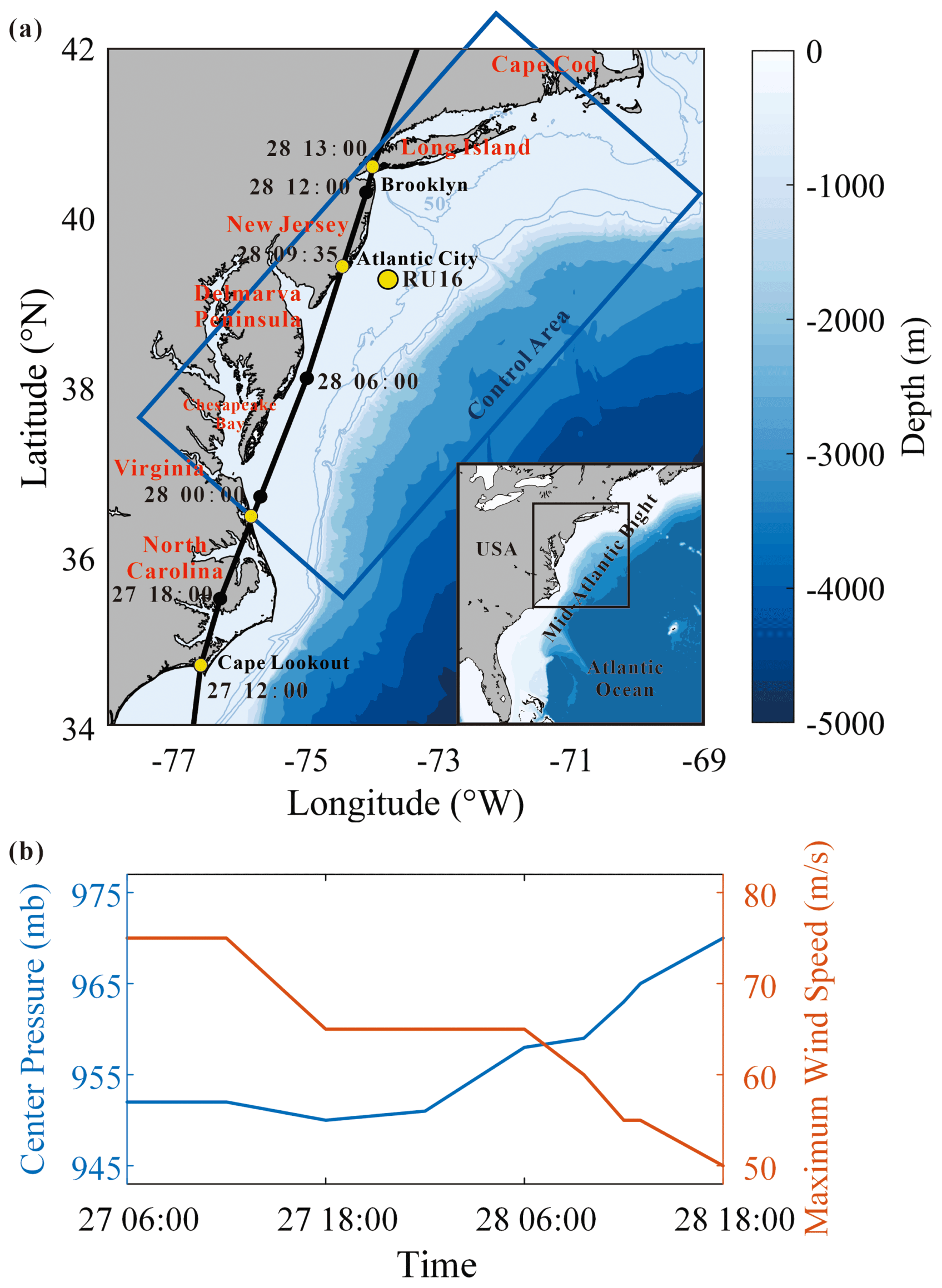
Figure 1 (a) Map of the MAB region. The best track of Hurricane Irene (2011) reported by Avila and Cangialosi (2011) is shown by a black line. Reanalysis data provided by H^*WIND show a similar track as Avila and Cangialosi (2011) and are thus omitted. The mean position of Glider RU16 is marked by a yellow circle. The control domain defined in Sect. 4 is marked by a blue box. (b) Time series of center pressure and 10 m maximum wind speed of Hurricane Irene reported by Avila and Cangialosi (2011).

In this study, we pay close attention to the NIC induced by Hurricane Irene (2011). Hurricane Irene (2011) crossed over the Mid-Atlantic Bight (MAB), a coastal region of the North Atlantic extending from Cape Cod, Massachusetts, to Cape Lookout, North Carolina, USA, as shown in Fig. 1a. Before the hurricane event, seawater stratification in MAB was quite strong due to the cold pool effect (Lentz, 2017), and the temperature difference between the surface and the bottom exceeded 10 ^∘C. The vertical gradient of the temperature should also be very large because previous studies showed that the thermocline in the shelf region was rather thin; for instance, the thermocline was less than 5 m in the place where water depth was around 40 m (Glenn et al., 2016; Seroka et al., 2017). During the passage of Hurricane Irene (2011), a network of high-frequency (HF) radars measured the surface currents in MAB (Roarty et al., 2010). Meanwhile, a Slocum glider launched near New Jersey measured the vertical profiles of the temperature and salinity (Schofield et al., 2010). The combination of valuable field data and effective numerical techniques then provided an opportunity to achieve a comprehensive study of the NICs generated by this hurricane event.

2 Numerical model

2.1 Basic equations

In this study, the ocean responses to Hurricane Irene (2011) are studied using the Regional Oceanic Modeling System (ROMS) (Shchepetkin and McWilliams, 2005; Haidvogel et al., 2008; Hedstrom et al., 2021). ROMS deals with the Reynolds-averaged N–S equations in the σ-coordinate system (Freeman et al., 1972). Specifically, the Cartesian coordinate z is replaced by σ based on a general relation $\mathit{\chi }\left(\mathit{\sigma }\right)=\left(z-\mathit{\eta }\right)/D$, where η is the vertical displacement of the free surface and D is the instantaneous water depth, while χ(σ) is a stretching function introduced for grid refinement. In the σ-coordinate system the Reynolds-averaged N–S equations may finally be expressed as follows.

$$\begin{array}{}\text{(1)}& {\displaystyle \frac{\partial \mathit{\xi }}{\partial t}}+{\displaystyle \frac{\partial \left(\mathit{\xi }u\right)}{\partial x}}+{\displaystyle \frac{\partial \left(\mathit{\xi }v\right)}{\partial y}}+{\displaystyle \frac{\partial \left(\mathit{\xi }\mathit{\omega }\right)}{\partial \mathit{\sigma }}}=\mathrm{0}\text{(2)}& {\displaystyle }\begin{array}{rl}& {\displaystyle \frac{\partial \left(\mathit{\xi }u\right)}{\partial t}}+{\displaystyle \frac{\partial \left(\mathit{\xi }uu\right)}{\partial x}}+{\displaystyle \frac{\partial \left(\mathit{\xi }uv\right)}{\partial y}}+{\displaystyle \frac{\partial \left(\mathit{\xi }u\mathit{\omega }\right)}{\partial \mathit{\sigma }}}-f\mathit{\xi }v+{\displaystyle \frac{\mathit{\xi }}{\mathit{\rho }}}{\displaystyle \frac{\partial p}{\partial x}}\\ & =-g\mathit{\xi }\left(\mathit{\chi }{\displaystyle \frac{\partial D}{\partial x}}+{\displaystyle \frac{\partial \mathit{\eta }}{\partial x}}\right)+{\displaystyle \frac{\partial }{\partial \mathit{\sigma }}}\left({\displaystyle \frac{\mathit{\nu }}{\mathit{\xi }}}{\displaystyle \frac{\partial u}{\partial \mathit{\sigma }}}\right)\\ & +{\displaystyle \frac{\partial }{\partial x}}\left(\mathit{\xi }{\mathit{\nu }}^{\prime }{\displaystyle \frac{\partial u}{\partial x}}\right)+{\displaystyle \frac{\partial }{\partial y}}\left(\mathit{\xi }{\mathit{\nu }}^{\prime }{\displaystyle \frac{\partial u}{\partial y}}\right)\end{array}\text{(3)}& {\displaystyle }\begin{array}{rl}& {\displaystyle \frac{\partial \left(\mathit{\xi }v\right)}{\partial t}}+{\displaystyle \frac{\partial \left(\mathit{\xi }uv\right)}{\partial x}}+{\displaystyle \frac{\partial \left(\mathit{\xi }vv\right)}{\partial y}}+{\displaystyle \frac{\partial \left(\mathit{\xi }v\mathit{\omega }\right)}{\partial \mathit{\sigma }}}+f\mathit{\xi }u+{\displaystyle \frac{\mathit{\xi }}{\mathit{\rho }}}{\displaystyle \frac{\partial p}{\partial y}}\\ & =-g\mathit{\xi }\left(\mathit{\chi }{\displaystyle \frac{\partial D}{\partial y}}+{\displaystyle \frac{\partial \mathit{\eta }}{\partial y}}\right)+{\displaystyle \frac{\partial }{\partial \mathit{\sigma }}}\left({\displaystyle \frac{\mathit{\nu }}{\mathit{\xi }}}{\displaystyle \frac{\partial v}{\partial \mathit{\sigma }}}\right)\\ & +{\displaystyle \frac{\partial }{\partial x}}\left(\mathit{\xi }{\mathit{\nu }}^{\prime }{\displaystyle \frac{\partial v}{\partial x}}\right)+{\displaystyle \frac{\partial }{\partial y}}\left(\mathit{\xi }{\mathit{\nu }}^{\prime }{\displaystyle \frac{\partial v}{\partial y}}\right)\end{array}\text{(4)}& {\displaystyle }\mathrm{0}=-{\displaystyle \frac{\mathrm{1}}{\mathit{\rho }}}{\displaystyle \frac{\partial p}{\partial \mathit{\sigma }}}-g\mathit{\xi }\text{(5)}& {\displaystyle }\begin{array}{rl}& {\displaystyle \frac{\partial \left(\mathit{\xi }C\right)}{\partial t}}+{\displaystyle \frac{\partial \left(\mathit{\xi }uC\right)}{\partial x}}+{\displaystyle \frac{\partial \left(\mathit{\xi }vC\right)}{\partial y}}+{\displaystyle \frac{\partial \left(\mathit{\xi }\mathit{\omega }C\right)}{\partial \mathit{\sigma }}}\\ & ={\displaystyle \frac{\partial }{\partial \mathit{\sigma }}}\left({\displaystyle \frac{\mathit{\kappa }}{\mathit{\xi }}}{\displaystyle \frac{\partial C}{\partial \mathit{\sigma }}}\right)+{\displaystyle \frac{\partial }{\partial x}}\left(\mathit{\xi }{\mathit{\kappa }}^{\prime }{\displaystyle \frac{\partial C}{\partial x}}\right)+{\displaystyle \frac{\partial }{\partial y}}\left(\mathit{\xi }{\mathit{\kappa }}^{\prime }{\displaystyle \frac{\partial C}{\partial y}}\right)\end{array}\end{array}$$

Here, $\mathit{\xi }=\partial z/\partial \mathit{\sigma }=D\left(\partial \mathit{\chi }/\partial \mathit{\sigma }\right)$; u, v, and ω are the velocity components in the x, y, and σ directions, respectively; C stands for the potential temperature T or salinity S; p is the seawater pressure; ρ is the density of the seawater; f=2Ωsin ϕ is the Coriolis parameter with $\mathrm{2}\mathrm{\Omega }=\mathrm{1.458}\times {\mathrm{10}}^{-\mathrm{4}}$ s⁻¹ and ϕ being the latitude; ν and κ are the diffusion coefficients for momentum and potential temperature or salinity, respectively, in the vertical direction; and ν^′ and κ^′ are those in the horizontal directions. Note that Eq. (1) is the continuity equation, Eqs. (2) and (3) are equations of motion in two horizontal directions, Eq. (4) is the hydrostatic assumption, and Eq. (5) is the advection–diffusion equation of the potential temperature or the salinity. The density of the seawater ρ is determined following the equation of state proposed by Jackett and McDougall (1995):

$$\begin{array}{}\text{(6)}& \mathit{\rho }\left(S,T,p\right)={\displaystyle \frac{{\mathit{\rho }}_{\mathrm{0}}}{\mathrm{1}-p/K\left(S,T,p\right)}},\end{array}$$

where ${\mathit{\rho }}_{\mathrm{0}}=\mathit{\rho }\left(S,T,\mathrm{0}\right)$ is the seawater density at the standard atmospheric pressure, and $K\left(S,T,p\right)$ is the bulk modulus; both are given by Jackett and McDougall (1995).

The vertical mixing is known to play an important role in determining the structure of a NIC, so it must be properly evaluated. In this study, we consider $\mathit{\nu }={\mathit{\nu }}_{\mathrm{0}}+{\mathit{\nu }}_{\mathrm{e}}$ and $\mathit{\kappa }={\mathit{\kappa }}_{\mathrm{0}}+{\mathit{\kappa }}_{\mathrm{e}}$, in which ν₀ and κ₀ are the molecular viscosity and diffusivity of the seawater set to ${\mathit{\nu }}_{\mathrm{0}}={\mathrm{10}}^{-\mathrm{5}}$ m² s⁻¹ and ${\mathit{\kappa }}_{\mathrm{0}}={\mathrm{10}}^{-\mathrm{6}}$ m² s⁻¹ following previous suggestions (Xu et al., 2002; Li et al., 2007; Lentz, 2017), while ν_e and κ_e are the eddy viscosity and diffusivity determined by the conventional k-ε turbulence model (see Rodi, 1987, and Umlauf and Burchard, 2003, for a detailed description), a widely employed model that demonstrated good performance in simulating various oceanographic processes (Olabarrieta et al., 2011; Toffoli et al., 2012; Zhang et al., 2018).

Horizontal mixing is included in Eqs. (2), (3), and (5), though it has been pointed out to play a relatively insignificant role in simulating the response of the stratified ocean to a hurricane compared to vertical mixing (Li et al., 2007; Zhai et al., 2009; Dorostkar et al., 2010). In the ocean basin of the present interest, the horizontal diffusion coefficient was estimated to be of the order of 10 m² s⁻¹ under extreme conditions, e.g., TC conditions (Allahdadi, 2014; Mulligan and Hanson, 2016). Thus, we take ${\mathit{\nu }}^{\prime }={\mathit{\kappa }}^{\prime }=\mathrm{10}$ m² s⁻¹ in the present study for simplicity to simulate the ocean response to Hurricane Irene.

2.2 Computational conditions

In order to fully capture the NIC induced by Hurricane Irene (2011), our computational domain covers the entire MAB region of the US East Coast extending from Cape Cod, Massachusetts, to Cape Lookout, North Carolina. The computational domain is discretized into 35 layers with refinement near the surface and covered with a 5 km × 5 km grid in the horizontal plane. The 1 arcmin bathymetry data are obtained from the ETOPO1 global relief model (Amante and Eakins, 2009) and resampled to a resolution of 5 km. The simulation starts from 20 August, 1 week before the hurricane event, and lasts for a period of 16 d. The time step is set to 1 min.

The initial and open boundary conditions of the seawater temperature and salinity, the ocean flow velocities, and the sea surface elevation are all from the Hybrid Coordinate Ocean Model (HYCOM, https://www.hycom.org/, last access: 30 June 2022) with a resolution of $\mathrm{1}/\mathrm{12}$^∘ in space and 3 h in time (Cummings, 2005; Chassignet et al., 2007; Naval Research Laboratory, 2012). The initial stratification in HYCOM is examined through a comparison with the 4D data provided by the Experimental System for Predicting Shelf and Slope Optics (ESPreSSO, https://tds.marine.rutgers.edu/thredds/roms/catalog.html, last access: 30 June 2022). Seven tidal constitutes (M2, S2, N2, K2, O1, K1, Q1) included in the simulation are derived from the ADvanced CIRCulation model (ADCIRC, https://adcirc.org/, last access: 30 June 2022) (Luettich et al., 2015). Daily inflows from the 11 largest rivers, containing the Susquehanna River, Delaware River, Hudson River, and Potomac River, among others, are obtained from the United States Geological Survey (USGS, 2022, https://waterdata.usgs.gov/nwis/uv/?referred_module=sw, last access: 30 June 2022). The so-called radiation-nudging condition is adopted at the open boundaries (Marchesiello et al., 2001). A wet-and-dry option is activated at coastal boundaries (Warner et al., 2013). The seabed boundary condition is required to satisfy

$$\begin{array}{}\text{(7)}& \mathit{\nu }{\displaystyle \frac{\partial \mathit{u}}{\partial z}}={\mathit{\tau }}_{\mathrm{b}}=\mathit{\rho }{\left[{\displaystyle \frac{\mathit{\lambda }}{\ln \left(\mathrm{\Delta }z/z_{\mathrm{0}}\right)}}\right]}^{\mathrm{2}}\left|{\mathit{u}}_{\mathrm{b}}\right|{\mathit{u}}_{\mathrm{b}},\end{array}$$

where τ_b is the bottom friction; λ is the von Karman constant, u_b is the fluid velocity at the center of the bottom layer, Δz is the distance between the center of the bottom layer and the seabed, and z₀ is the bottom roughness, which is set to 0.02 m in MAB following Churchill et al. (1994).

The hurricane wind forcing required in this study can be obtained from two sources, i.e., H^*WIND data, with a spatial resolution of 6 km and a temporal resolution of 6 h, published by the Atlantic Oceanographic and Meteorological Laboratory, National Oceanic and Atmospheric Administration (AOML/NOAA) (https://www.rms.com/event-response/hwind, last access: 20 December 2019) (Powell et al., 1998; RMS, 2019), and North American Mesoscale (NAM) data, with a spatial resolution of 12 km and a temporal resolution of 3 h, provided by the National Centers for Environmental Prediction (NCEP, 2012) (https://tds.marine.rutgers.edu/thredds/catalog/met/ncdc-nam-3hour/catalog.html, last access: 30 June 2022) (Janjic et al., 2004). In our computation, the former is used between 26 and 31 August (during the hurricane event) because it has better accuracy in capturing the maximum wind speed, while the latter is used during other periods of the simulation. Reanalysis data for other atmospheric forcing, such as the surface air temperature, air pressure, relative humidity, radiation, and precipitation, are also available from NAM for determining the surface buoyancy fluxes.

In this study, the boundary layer effect on the near-inertial current is not directly considered. The driving effect of the airflow on the near-inertial current is reflected by adding a wind drag on the ocean surface. The wind drag τ_s, which is measure of the vertical flux of horizontal momentum, can be estimated through (Fairall et al., 1996)

$$\begin{array}{}\text{(8)}& {\mathit{\tau }}_s={\mathit{\rho }}_{\mathrm{a}}{C}_{\mathrm{d}}{u}_{\mathrm{10}}^{\mathrm{2}},\end{array}$$

where ρ_a is the density of the air, C_d is the drag coefficient, and u₁₀ is the horizontal wind speed at the 10 m level. Traditionally, the drag coefficient C_d is expressed as a linear function of the wind speed. In this study, we adopt a more advanced formula that fits the numerical results obtained with an improved wave boundary layer model under extreme wind conditions (Chen and Yu, 2016; Chen et al., 2018; Xu and Yu, 2021):

$$\begin{array}{}\text{(9)}& C_{\mathrm{d}}=C_{\mathrm{dw}}+{\displaystyle \frac{C_{\mathrm{d}\mathrm{0}}-C_{\mathrm{dw}}}{(W_{\mathrm{0}}-W{)}^{\mathrm{2}}}}(u_{\mathrm{10}}-W{)}^{\mathrm{2}},\end{array}$$

where C_d0 is a threshold value set to 0.001 for the wind stress at $u_{\mathrm{10}}\le W_{\mathrm{0}}=\mathrm{5}$ m s⁻¹, C_dw is the saturated wind stress coefficient, and W is the saturation wind speed. We have the following.

$$\begin{array}{}\text{(10)}& {\displaystyle }{C}_{\mathrm{dw}}=\left\{\begin{array}{ll}-\mathrm{1.86}\times {\mathrm{10}}^{-\mathrm{4}}\ln \frac{gD}{W_{\mathrm{D}}}+\mathrm{0.0025}& \frac{gD}{W_{\mathrm{D}}}\le \mathrm{3}\\ & \\ \mathrm{0.00225}& \frac{gD}{W_{\mathrm{D}}}>\mathrm{3}\end{array}\right.\text{(11)}& {\displaystyle }W=\left\{\begin{array}{ll}\mathrm{4.64}\ln \left(\frac{gD}{W_{\mathrm{D}}}\right)+\mathrm{42.6}& \frac{gD}{W_{\mathrm{D}}}\le \mathrm{0.6}\\ & \\ W_{\mathrm{D}}& \frac{gD}{W_{\mathrm{D}}}>\mathrm{0.6}\end{array}\right.\end{array}$$

Here, W_D set to 40 m s⁻¹ is the saturation wind speed in deep water. Except for the momentum flux, other air–sea fluxes, e.g., the sensible heat flux and the latent heat flux, are determined based on the conventional bulk parameterization scheme (see Fairall et al., 1996, for detailed description). The sea surface boundary condition is then required to satisfy

$$\begin{array}{}\text{(12)}& \mathit{\nu }{\displaystyle \frac{\partial \mathit{u}}{\partial z}}={\mathit{\tau }}_s.\end{array}$$

2.3 Observational data

During the passage of Hurricane Irene (2011), a network of high-frequency (HF) radars measured the surface currents and a Slocum glider launched near New Jersey measured the vertical profiles of the temperature and salinity (Roarty et al., 2010; Schofield et al., 2010). The measured data are used to verify the computational results in this study. In fact, they have been widely used in previous studies (Glenn et al., 2016; Seroka et al., 2016, 2017).

HF radars in the Mid-Atlantic Regional Association's Coastal Ocean Observing System are able to observe the surface currents. The recorded data have a temporal resolution of 1 h and a spatial resolution of 6 km, and they are assumed to be measured at an effective depth of around 2.7 m below the ocean surface based on Roarty et al. (2020). The data cover the MAB area from the coast to the shelf break. HF radar measures the radial component of ocean surface currents based on the Doppler effect. The surface currents are determined by combining overlapping radials from different radars in the observational network using an optimal interpolation method (Roarty et al., 2010; Zhang et al., 2018). “Coverage” is defined to represent how many overlapping radials are combined and is thus closely related to the accuracy of data at a given point. Previous studies pointed out that the data are rather reliable when the coverage is larger than 90 % (Roarty et al., 2010; Kohut et al., 2012). Intrinsic HF radar uncertainty has been estimated to be of the order of 5 cm s⁻¹ (Brunner and Lwiza, 2020), indicating a relative error of around 0.10 in regards to the surface current velocities. When compared with ADCP, the root mean square (rms) difference of HF radar is only within 8 cm s⁻¹ (Roarty et al., 2010; Kohut et al., 2012; Roarty et al., 2020). In this study, HF radar data are directly obtained from http://tds.marine.rutgers.edu/thredds/dodsC/cool/codar/totals/5Mhz_6km_realtime_fmrc/Maracoos_5MHz_6km_Totals-FMRC_best.ncd.html (last access: 30 June 2022) (RUCOOL, 2022) and spatially interpolated to the locations of our interest. All the data within the shelf break are found to be quite reliable since the coverage there is larger than 90 %. Note that the data outside the shelf break have a low coverage of 60 %–90 %. Though we use all the data as they are, we must remind readers that the data outside the shelf break should be viewed with caution.

Glider RU16 is an autonomous underwater vehicle of the Rutgers Slocum glider (Schofield et al., 2007, 2010) platform developed by Teledyne Webb Research and has demonstrated to be advantageous in marine monitoring, particularly under extreme weather conditions (Glenn et al., 2016; Miles et al., 2017; Zhang et al., 2018). It was equipped with a Sea-Bird un-pumped conductivity, temperature, and depth (CTD) sensor and could thus measure not only the vertical profiles of the seawater temperature and the salinity but also the water depth. It was programmed to move vertically through the water column, collect data every 2 s, and surface at a 3 h interval to provide high-temporal-resolution data (Schofield et al., 2007; Glenn et al., 2016; Seroka et al., 2016). The RU16 dataset has been widely used and well verified by previous authors (Glenn et al., 2016; Seroka et al., 2016, 2017). Therefore, it is used as it is in this study. The dataset is available at http://tds.marine.rutgers.edu/thredds/dodsC/cool/glider/mab/Gridded/20110810T1330_epa_ru16_active.nc.html (last access: 30 June 2022) (RUCOOL, 2016).

3 Ocean responses to Hurricane Irene

3.1 Effect of the hurricane on ocean surface flow

As shown in Fig. 1, Hurricane Irene (2011) entered the Mid-Atlantic Bight (MAB) area of the present interest at Cape Lookout, North Carolina, as a Category-1 event at 12:00 on 27 August 2011 (UTC, the same below) with a maximum sustained wind (MSW) of over 38 m s⁻¹. It continued to move northeastward and made landfall at Atlantic City, New Jersey, at 09:35 on 28 August with an MSW of around 30 m s⁻¹. During its motion in the MAB area of our interest, the radius of the hurricane wind field (the area with wind speed ≥32.9 m s⁻¹) reached a large value of 140 km (Avila and Cangialosi, 2011).

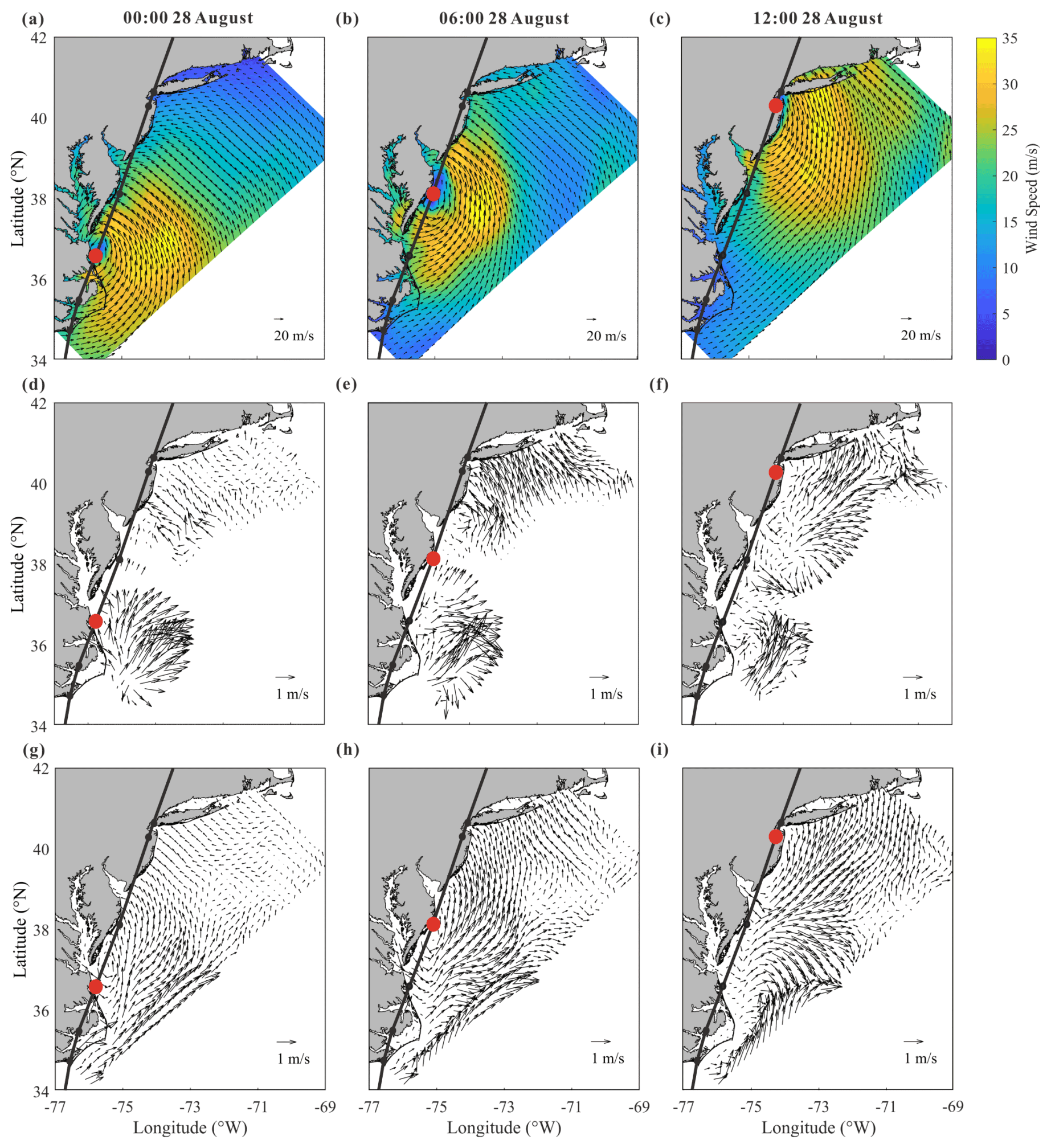
Figure 2 Snapshots of (a–c) the 10 m wind provided by H^*WIND, (d–f) computed current velocity of the surface layer, and (g–i) observed current velocity of the surface layer at (a, d, g) 00:00, (b, e, h) 06:00, and (c, f, i) 12:00 on 28 August during the passage of Hurricane Irene (2011). Note that the best track of the hurricane reported by Avila and Cangialosi (2011) is shown by black lines, while the hurricane center is shown by red circles.

Figure 2 provides snapshots of the wind as well as the computed and observed currents in the MAB area at 00:00, 06:00, and 12:00 on 28 August 2011, respectively. Note that 00:00 and 12:00 correspond to the time when Hurricane Irene entered and left the area of our interest, respectively. The wind field is plotted from the H^*WIND data, while the field currents are obtained by the HF radars and detided with MATLAB toolbox T_TIDE (Pawlowicz et al., 2002).

The computed current velocity of the surface layer, as shown in Fig. 2d–f, is compared with the observed one, as shown in Fig. 2g–i, to verify the reliability of the numerical model presented in this study. At 00:00 on 28 August, it is numerically demonstrated that currents rotating counterclockwise with a magnitude of over 1 m s⁻¹ are rapidly generated by the wind near the hurricane center (Fig. 2d). In the observed results, though there are significant data missing near the hurricane center, northeastward currents can still be identified in the offshore waters along the North Carolina coast (Fig. 2g) and are in reasonable agreement with the computed current field. Moreover, both computational and observational results support the fact that the onshore wind (Fig. 2a) on the front side of the hurricane drives an onshore current with a magnitude of 0.4 m s⁻¹ along the northern MAB, especially in the nearshore area of New Jersey (Fig. 2d and g). At 06:00, Hurricane Irene arrived at the offshore waters of the Delmarva Peninsula. In spite of the field data missing, the rotating currents induced by the hurricane wind can be clearly recognized in both computed and observed results in the nearshore area of New Jersey (Fig. 2e and h). In addition, relatively strong onshore currents with a magnitude of over 1 m s⁻¹ are observed near Long Island and are also well represented in the numerical results (Fig. 2e). At 12:00, i.e., the time when the hurricane left the area of our interest, the counterclockwise-rotating currents are still formed near the hurricane center as demonstrated by both computational and observational results (Fig. 2f and i). At the same time, clockwise-rotating currents are shown to have been generated near the Delmarva Peninsula in the southern MAB after the hurricane passed over. This fact is certainly confirmed by both computed and observed results, indicating that near-inertial currents are activated after the hurricane event. Therefore, it becomes evident that the rotating wind of the hurricane immediately forces a rotating current in the surface layer of the ocean and induces an inertial current rotating in the opposite direction shortly after the hurricane passes over. It is also worthwhile to emphasize that, in general, the numerical results obtained with the present model agree fairly well with observed data.

3.2 Effect of the hurricane on vertical stratification and sea surface cooling

Shown in Fig. 3a is the vertical profile of the seawater temperature measured by Glider RU16 launched off the New Jersey coast. It provides a good chance for us to validate the response of stratification to the hurricane event, which is likely one of the most important results of hurricane–ocean interaction. In Fig. 3a, it is seen that the mixed layer off the New Jersey coast was quite thin, with a thickness of less than 10 m, before the hurricane event. A strong stratification was clearly formed over a water depth of 40 m, with a surface temperature of 24 ^∘C and a bottom temperature of 10 ^∘C. When the hurricane center passed over the position of Glider RU16 at around 09:30 on 28 August, the thickness of the mixed layer rapidly increased to nearly 30 m, while the surface temperature decreased by more than 5 ^∘C, indicating the occurrence of a strong mixing process. By plotting the time series of the squared buoyancy frequency N based on the measured data, expansion of the mixed layer due to the hurricane event may be more vividly demonstrated (Fig. 3c).

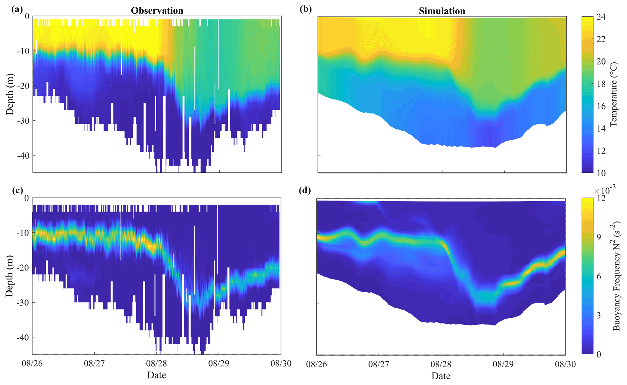
Figure 3 Time series of the vertical profiles of (a, b) the temperature and (c, d) the squared buoyancy frequency obtained from (a, c) Glider RU16 and the (b, d) numerical model.

Figure 3b and d present the computed results for the vertical distribution of seawater temperature obtained by virtually setting a measuring point moving with the glider in the real situation. The numerical results show a similar variation of the stratification pattern as observed before and during the hurricane event. They reproduce both extension of the mixed layer and cooling of the sea surface, indicating that the numerical model is capable of describing the development and destruction of ocean stratification. However, a sea surface cooling of about 4 ^∘C obtained by the numerical model is a little smaller than 6–7 ^∘C observed by the glider in the field, probably due to the inaccurate setting of the initial bottom temperature in the computation. Discrepancies of the squared buoyancy frequency N were also found in the thermocline (Fig. 3c), where the temperature varied most dramatically. They are probably caused by the inaccurate setting of the initial temperature profile. In fact, the initial condition for the bottom temperature in HYCOM is somehow higher (about 4 ^∘C) than the observed value in the field if Fig. 3a and b are compared. To correct this system error, the real-time profile obtained from RU16 is used for a nudging process in computation; i.e., the model temperature and salinity fields are forced to nudge toward observed data (see Thyng et al., 2021, for a detailed description).

The sea surface temperatures (SSTs) before and after the hurricane event are further compared in Fig. 4 (obtained from The Advanced Very High Resolution Radiometer – AVHRR, https://tds.marine.rutgers.edu/thredds/cool/avhrr/catalog.html?dataset=cool-avhrr-bigbight-2011, last access: 30 June 2022) (RUCOOL, 2011). Before the hurricane event, both observed and computed SSTs show similar patterns; i.e., the SST decreases with the increasing latitude. After the hurricane passage, the strong mixing and cooling mainly take place in shallow waters, where the initial stratification is strong (Zhang et al., 2016), especially near New Jersey and Long Island. However, the cooling is not prominent in shallow waters near North Carolina. In fact, it has been reported that the SST in this region decreased and then recovered to its pre-hurricane level within only 1 d (Seroka et al., 2016). In fact, the HYCOM data showed that the initial bottom temperature near North Carolina was as high as 18 ^∘C. Considering that sea surface cooling was positively related to the vertical temperature gradient (Shay and Brewster, 2010; Vincent et al., 2012; Zhang et al., 2016), the small amount of cold pool water in this region may have caused insignificant cooling and fast recovery.

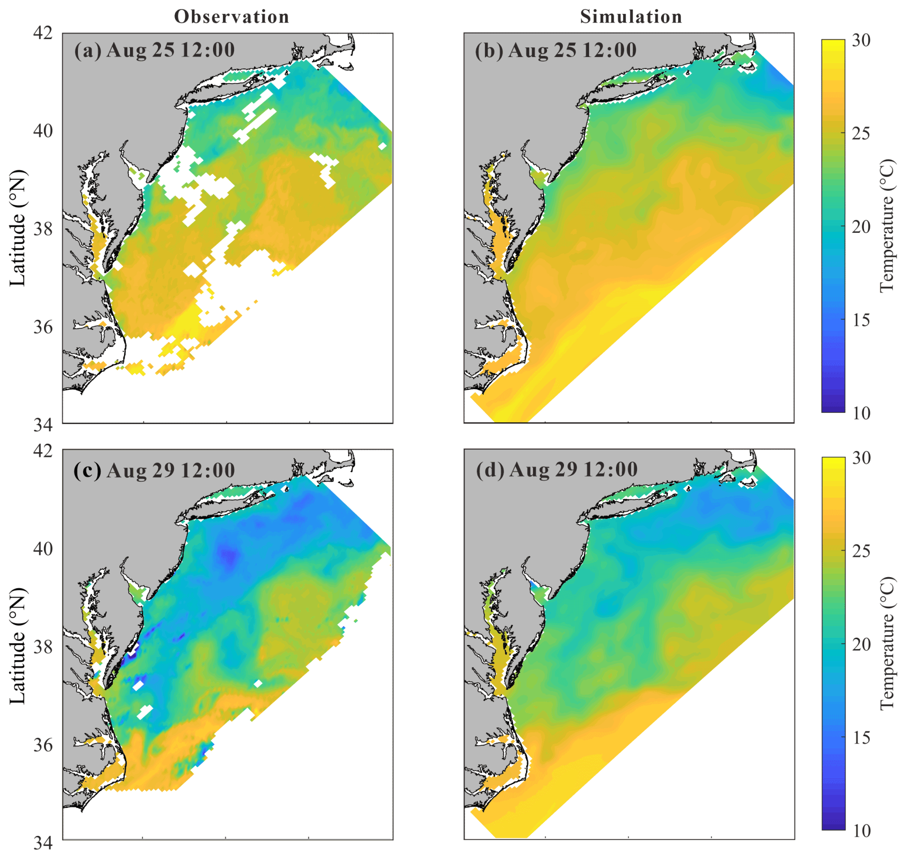
Figure 4 Sea surface temperature on 25 August at 12:00 before the hurricane event (a, b) and on 29 August at 12:00 after the hurricane event (c, d) from (a, c) observed data and the (b, d) numerical model.

It should be pointed out that the computed SST cooling is 3–4 ^∘C smaller than the observed one, which could also be explained by the inaccurate initial condition obtained from HYCOM. The HYCOM bottom temperature is somehow higher than actual, which could lead to the underestimation of the SST cooling. Therefore, we use the real-time SST data obtained from AVHRR for the nudging process in computation to correct this system error (Thyng et al., 2021), considering that the accuracy of the initial stratification could obviously affect the modeling of the mixing process. Note that the error is mainly caused by the discrepancy in initial settings but not defects in the numerical method. Thus, this error could be calibrated to a certain extent and would not affect the reliability of subsequent analysis, e.g., energy budget analysis.

3.3 Characteristics of NIC

To have a general understanding of the NICs in the MAB area induced by Hurricane Irene (2011), a network of 30 stations aligned on five cross-shore sections from south to north is introduced in this study to cover the area of our interest as shown in Fig. 5, similar to Zhang et al. (2018). In each section, six stations are placed in the cross-shore direction from the shore side to the deep ocean, where water depths are around 30, 50, 75, 120, 220, and 1000 m, respectively. Note that the most offshore stations are located outside the shelf break.

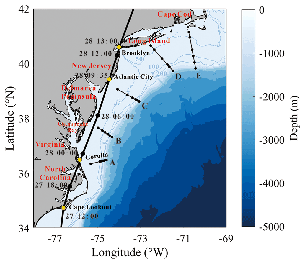
Figure 5 Five virtual sections marked by short black lines.

The velocity of NIC is obtained from the total current velocity by first excluding the tidal components and then passing it through a Butterworth filter with the frequency band of 0.8–1.2 f₀, an effective approach proposed by Hormann et al. (2014), Zhang et al. (2018), and Kawaguchi et al. (2020). Shown in Fig. 6 are the time series of the surface velocity of the NIC component in the cross-shore direction interpolated to 30 stations during the time period of our study (16 d from 20 August to 5 September). Results obtained with the numerical model are also presented. The alongshore component is similar to the cross-shore component and thus omitted here. Intuitively, the numerical results are in reasonably good agreement with the HF radar data. For a further discussion we define the near-inertial kinetic energy (NIKE) in the following way:

$$\begin{array}{}\text{(13)}& E^{\prime }={\displaystyle \frac{\mathrm{1}}{\mathrm{2}}}{\mathit{\rho }}_{\mathrm{0}}{\left|{\mathit{u}}^{\prime }\right|}^{\mathrm{2}},\end{array}$$

where ρ₀ is the velocity of the NIC, and u^′ is the seawater density at the standard atmospheric pressure. A phase-corrected relative mean square error may then be introduced to describe the difference between the computed and observed NIKE:

$$\begin{array}{}\text{(14)}& \mathrm{\Delta }={\displaystyle \frac{\underset{\mathit{\tau }}{min}{\int }_{t_{\mathrm{0}}}^{t_{\mathrm{1}}}\left[E_{\mathrm{O}}^{\prime }\right(t)-E_{\mathrm{C}}^{\prime }(t-\mathit{\tau }){]}^{\mathrm{2}}\mathrm{d}t}{\sqrt{{\int }_{t_{\mathrm{0}}}^{t_{\mathrm{1}}}\left[E_{\mathrm{O}}^{\prime }\right(t){]}^{\mathrm{2}}\mathrm{d}t}\sqrt{{\int }_{t_{\mathrm{0}}}^{t_{\mathrm{1}}}\left[E_{\mathrm{C}}^{\prime }\right(t){]}^{\mathrm{2}}\mathrm{d}t}}},\end{array}$$

where $E_{\mathrm{O}}^{\prime }\left(t\right)$ and $E_{\mathrm{C}}^{\prime }\left(t\right)$ are the observed and computed NIKE time series, respectively; [t₀,t₁] is the duration when the hurricane-induced NICs are prominent, which is taken to be from 25 August to 4 September in this study; and τ is a time shift for eliminating the phase error. We calculate Δ at all 30 stations. It is shown that Δ varies from 0.14–0.23 in most stations where the coverage is larger than 90 %. However, it is also necessary to mention that in several nearshore stations, i.e., A1, D1, and E1, Δ exceeds 0.3 because the NIC is too weak at these stations compared to the background currents. At the six stations outside the shelf break, e.g., at A6, C6, and D6, Δ even exceeds 0.5–0.6, implying that the HF radar data are less accurate outside the shelf with low coverage. As we mentioned in Sect. 2.3, the relative rms difference of HF radar data is around 0.10. Taking this intrinsic HF radar uncertainty into consideration, Δ = 0.14–0.23 in our study is quite acceptable. Therefore, we could conclude that our numerical results are in reasonably good agreement with the HF radar data. Inaccuracy in the numerical results of the NICs may come from the minor errors in the wind forcing data because they are very sensitively related; e.g., underestimation at C3–C6 before the hurricane event may come from the errors in low-resolution NAM data used in pre-hurricane periods. In addition, error in the initial wind data may cause insignificant phase discrepancies in B3–B6.

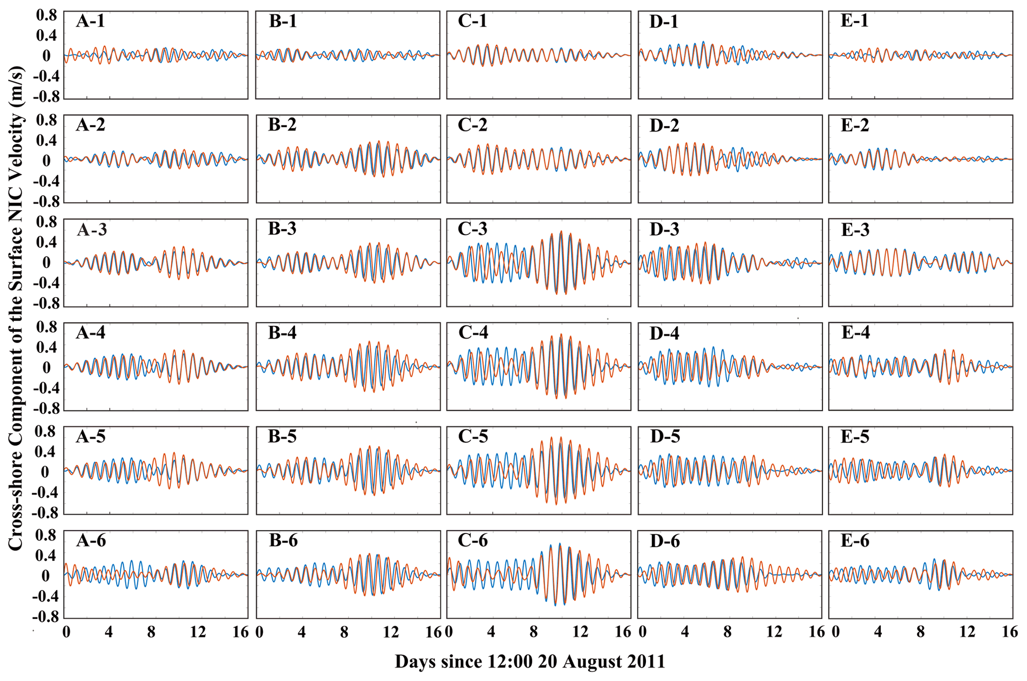
Figure 6 Time series of the NIC velocity in the surface layer obtained (blue line) by the HF radar and (orange line) with the numerical model at 30 stations along sections A–E.

In Fig. 6, it can be readily recognized that in the cross-shore direction from shallow to deep waters (i.e., station nos. 1–5 in the present study) the NIC velocity gradually increases by a factor of at least 3, e.g., from 0.15 to 0.6 m s⁻¹ in section C, which is consistent with conclusions in previous studies (Kim and Kosro, 2013; Yang et al., 2015; Rayson et al., 2015; Zhang et al., 2018). This is because NIC velocity in the nearshore region is restricted due to a combination of several factors presented by Chen and Xie (1997), Rayson et al. (2015), and Chen et al. (2017). Different from other studies, however, the NIC velocity in the deep waters (i.e., station no. 6 in the present study) is found to be not larger (or even smaller) than that near the shelf break. This is probably due to that fact that the track of Hurricane Irene (2011) was nearly attached to the shore during its motion in the area of our interest and the wind stress over the deep ocean was relatively small. From south to north, it is found that the NIC velocity in the middle regions, such as along section C, is larger than those in the south and north. By checking the numerical results, it is found that the stratification was only slightly destroyed during the hurricane event near section C compared to the adjacent sections, which thus provided a better environment for NIC generation (Yang et al., 2015; Shen et al., 2017).

To evaluate the relative importance of the near-inertial currents, the rotary spectra of the surface current velocity during the period of study (16 d) at different stations are shown in Fig. 7. The tidal flows corresponding to the major constituents M2, N2, and K1, obtained with ADCIRC, are also plotted. It is seen that the velocity of the NICs is of an equivalent magnitude to that of the M2 tidal current at the shallow-water stations where the water depth is about 30 m (section C was taken for an example, Fig. 7a). But, the velocity of the NICs is significantly larger than that of the tidal current in deeper regions (Fig. 7b, c). It may be necessary to point out that weak NICs are not limited to the most nearshore stations. In section D, for example, it is extended to a water depth of 75 m (station D3, Fig. 7d) due to the severe destruction of stratification. However, the stratification outside D3 was relatively well maintained due to the thicker mixed layer in these regions and the farther distance from the main hurricane track. As discussed in the previous subsection, the weak NICs in the nearshore area are closely related to the destruction of stratification by the strong mixing process associated with the hurricane event (Yang et al., 2015; Shen et al., 2017). However, this effect does not challenge the dominant role of NICs in deep waters.

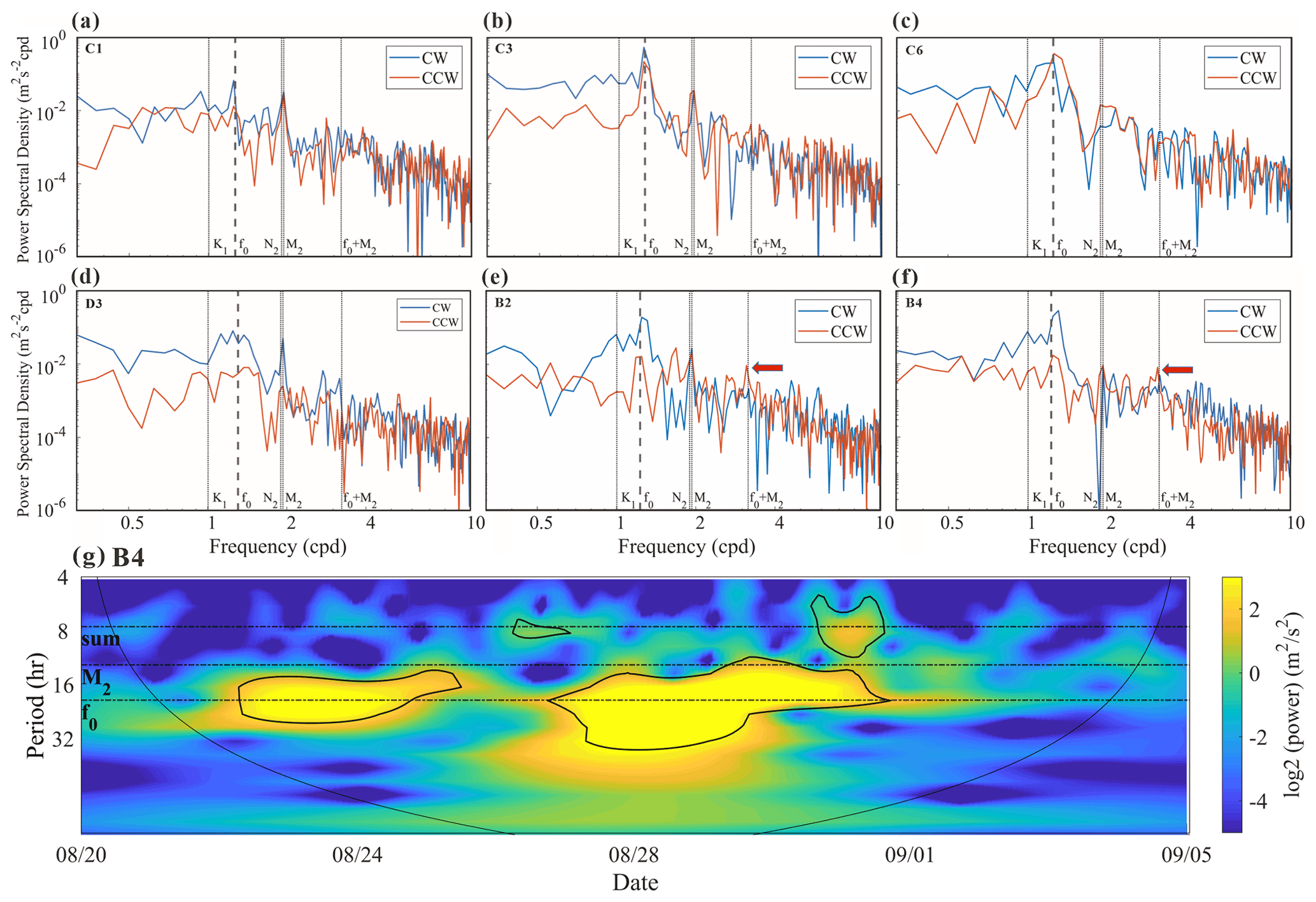
Figure 7 The rotary spectra of the current velocity in the surface layer during the simulation time (16 d) obtained by HF radar at stations (a) C1 (∼ 30 m), (b) C3 (∼ 75 m), (c) C6 (∼ 1000 m), (d) D3, (e) B2, and (f) B4. Clockwise and counterclockwise components of the current are shown by blue and orange lines, respectively (NICs are considered to be dominated by the clockwise component). The frequencies of the major tidal constituents M2, N2, and K1, the inertial frequency f0, and the sum frequency of M2 and f₀ are all marked by gray lines. (g) Wavelet power spectrum for the 10–30 m depth-averaged alongshore current component at station B4 (see Thiebaut and Vennell, 2010, for detailed description). Black contours indicate the 5 % significance level against red noise, and the arc line indicates the cone of influence.

Previous studies have reported that nonlinear wave–wave interaction could transfer energy from the M2 tide and NIC into a wave at the sum of their frequencies (fM2). The key mechanism is the coupling between the vertical shear in NIC and the vertical velocity due to the internal tide (Davies and Xing, 2003; Hopkins et al., 2014; Shen et al., 2017; Wu et al., 2020). Though the M2 tide is rather strong in shallow waters during the hurricane event (Fig. 7), nonlinear wave–wave interaction between the tidal current and the NIC could hardly be identified in most parts of MAB. Nevertheless, a peak of the energy spectrum seems to appear at the sum frequency fM2 for the surface velocity at stations B1 to B4 near the Delmarva Peninsula (B2 and B4 were taken as examples in Fig. 7e, f). The evolution of energy power at different frequencies for the middle-layer-averaged (i.e., 10–30 m) currents, where the flow shear is concentrated, is further demonstrated based on wavelet analysis (station B4 was taken as an example in Fig. 7g). A peak energy at the sum frequency fM2 is clearly identified after the hurricane passage. In fact, Sect. 4.2 in this paper will show that the strongest shear is found in offshore waters between the Delmarva Peninsula and New Jersey, i.e., near sections B and C (Fig. 9a). In addition, Brunner and Lwiza (2020) indicated that the most prominent M2 tide in the southern MAB is located off the Delmarva Peninsula (near section B), according to long-term observed data. Therefore, the vertical shear in NIC and the vertical velocity due to the M2 tide are more likely to be coupled in this region (i.e., near section B). However, this interaction only occurs in limited regions and thus would not influence the NIC evolution in most parts of MAB.

4 Near-inertial kinetic energy

4.1 Conservation of NIKE

For a description of the intensity of a NIC, the near-inertial kinetic energy (NIKE) may be defined in Eq. (13). Note that the NIKE is mainly gained from the wind power and dissipated due to a few mechanisms. Evolution of the vertically integrated NIKE within a water column from the sea bottom the ocean surface is thus governed by (Zhai et al., 2009)

$$\begin{array}{}\text{(15)}& \begin{array}{rl}\underset{-d}{\overset{\mathit{\eta }}{\int }}{\displaystyle \frac{\partial E^{\prime }}{\partial t}}\mathrm{d}z& ={\mathit{\tau }}_s\cdot {{\mathit{u}}^{\prime }}_s+{\mathit{\tau }}_{\mathrm{b}}\cdot {{\mathit{u}}^{\prime }}_{\mathrm{b}}-\underset{-d}{\overset{\mathit{\eta }}{\int }}{\mathit{\rho }}_{\mathrm{0}}{\mathit{\nu }}_e{\left|{\displaystyle \frac{\partial {\mathit{u}}^{\prime }}{\partial z}}\right|}^{\mathrm{2}}\mathrm{d}z\\ & -\underset{-d}{\overset{\mathit{\eta }}{\int }}\mathrm{\nabla }\cdot \left({\mathit{u}}^{\prime }{p}^{\prime }\right)\mathrm{d}z-\underset{-d}{\overset{\mathit{\eta }}{\int }}{\mathit{\rho }}^{\prime }g{w}^{\prime }\mathrm{d}z\\ & -\underset{-d}{\overset{\mathit{\eta }}{\int }}\mathrm{\nabla }\cdot \left(\mathit{U}{E}^{\prime }\right)\mathrm{d}z+\mathrm{others},\end{array}\end{array}$$

where ${{\mathit{u}}^{\prime }}_s$ and ${{\mathit{u}}^{\prime }}_{\mathrm{b}}$ are near-inertial velocities at the sea surface and bottom, respectively; U is the sub-inertial velocity; ρ^′ is the perturbation density, defined by ${\mathit{\rho }}^{\prime }=\mathit{\rho }-{\mathit{\rho }}_{\ast }$; ρ_∗ is the reference density, i.e., the density corresponding to a flattened stratification where the fluid is redistributed adiabatically to a stable and vertically uniform state from the actual condition (Holliday and McIntyre, 1981; Kang and Fringer, 2010; MacCready and Giddings, 2016); and p^′ is the perturbation pressure, defined by $p^{\prime }=g{\int }_z^{\mathit{\eta }}{\mathit{\rho }}^{\prime }\mathrm{d}z$. Terms on the right-hand side of Eq. (13) are the wind energy input, the dissipation due to bottom friction, the vertical diffusion due to turbulence, the horizontal divergence of near-inertial energy flux, the conversion between kinetic and potential energy, and the advection of NIKE by the sub-inertial flow. The last term “others” includes nonlinear transfer of energy between NICs and flows of other frequencies as well as the horizontal diffusion due to mixing. Note that the energy is integrated over the water column from $z=-d$ to the free surface z=η. In shallow waters, d is the actual water depth, while in deep waters, d is truncated to 200 m (i.e., the depth of the shelf break). When the bottom boundary is set at $z=-\mathrm{200}$ m, the bottom friction vanishes in Eq. (13) but a term related to the downward energy flux, i.e., $p^{\prime }{w}^{\prime }{\mathrm{|}}_{z=-\mathrm{200}\mathrm{m}}$, should be added.

For a general understanding, distribution of the depth-integrated NIKE averaged over a 10 d period from 25 August to 4 September is presented in Fig. 8a. The wind power integrated over the same period is plotted in Fig. 8b. It is clearly shown in Fig. 8a that the high-NIKE region is mainly located in the offshore waters of the Delmarva Peninsula and New Jersey rather than in the nearshore area. This distribution pattern is rather similar to that of the wind energy input, as presented in Fig. 8b, indicating that the NIKE was immediately gained from the wind power (Rayson et al., 2015; Shen et al., 2017; Zhang et al., 2018). In fact, the NIKE could also come from other processes apart from the wind energy input (Alford et al., 2016). Meanwhile, the wind energy input may also be transferred to energy of waves apart from NIC (Chen et al., 2017), which leads to differences between Figs. 8a and 7b.

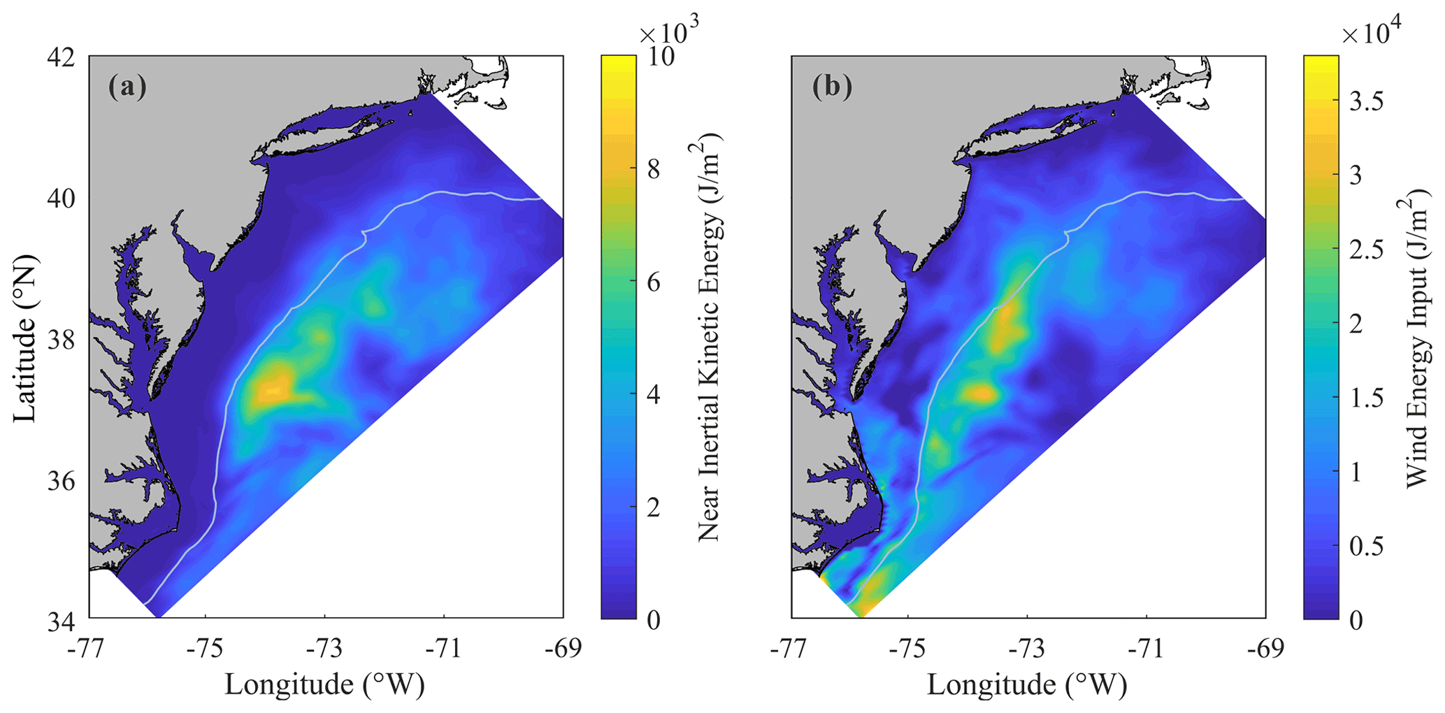
Figure 8 Spatial distribution of (a) depth-integrated near-inertial kinetic energy averaged over the 10 d period and (b) wind power input to NICs integrated over the 10 d period.

Table 1 The contribution of each mechanism to the energy budget. Percentages in parentheses refer to the ratio of each factor to wind energy input.

An important objective of the present study is to identify the mechanism of NIC development and decay. For this purpose, we consider a rectangular domain and separate it into deepwater region A (depth >200 m) and continental shelf region B (depth ≤200 m), as depicted in Fig. 1a. If the NICs are considered to be negligibly weak before and after Hurricane Irene (2011), we may try to find out how the wind power that drives the NICs during the hurricane event is balanced by comparing the accumulated contribution of different mechanisms. Performing an integration of each term in Eq. (13) with respect to time over 10 d from 25 August to 4 September and with respect to the horizontal coordinates over both deepwater region A and continental shelf region B, the contribution of each mechanism to the energy budget is obtained as shown in Table 1. It is clearly demonstrated that in the deepwater region, the wind energy input was basically balanced by the vertical diffusion due to turbulence (40 %) and a downward transfer of the near-inertial energy to the deep ocean (33 %). In the continental shelf region, the vertical diffusion due to turbulence dominated the dissipation of NIKE (nearly 70 %), while the bottom friction played a secondary role (24 %). It is worth mentioning that lateral divergence of NIKE should not be neglected in both shallow and deepwater regions under hurricane conditions (nearly 20 %), which is different from previous studies that focused on NICs under local wind conditions or in a broader research region across the whole North Atlantic (Chant, 2001; Zhai et al., 2009; Shen et al., 2017). Other processes, e.g., advection due to sub-inertial flows, only played a minor role. Note that the ratio of near-inertial energy decay to wind energy input exceeded 100 % in the continental shelf region, confirming that NIKE may be gained from other sources in addition to wind energy input in nearshore regions (Alford et al., 2016).

4.2 Decay of NIKE

The spatial distribution of the time-integrated energy dissipated through vertical diffusion due to turbulence is plotted in Fig. 9a. It is seen that a large amount of the dissipation occurred at the offshore side of the continental shelf (i.e., at the offshore side of the shallow region B), which does not coincide with the region where the wind energy input is intense as demonstrated in Fig. 8b. This implies that dissipation of NIKE is not mainly caused by an increased intensity of turbulence, which certainly takes place in a region where wind energy input achieves a high level (Zhai et al., 2009; Zhang et al., 2018). For a more detailed discussion, the averaged eddy viscosity ν_e and the averaged vertical shear rate of NIC ${\left|\partial {\mathit{u}}^{\prime }/\partial z\right|}^{\mathrm{2}}$ during the period of our study are presented in Figs. 9b and 8c. It is then confirmed that strong vertical shear also occurred at the outer half of the continental shelf. The eddy viscosity, however, has a completely different distribution. In conclusion, the vertical shear, which is known to be closely related to the ocean stratification (Shen et al., 2017), plays a crucial role in the turbulence diffusion. One of the most well-known and sharpest thermoclines in the world happens to exist in the coastal waters of MAB (Schofield et al., 2008; Lentz, 2017). It may be necessary to emphasize that, although the stratification in the shallowest water was totally destroyed during the hurricane event, as mentioned in Sect. 3, the seawater at the outer half of the continental shelf still partly maintained its stratification.

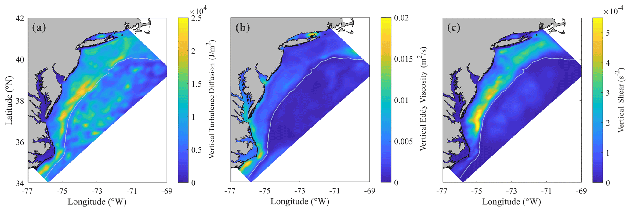
Figure 9 Spatial distribution of (a) depth-integrated vertical diffusion due to turbulence integrated over the 10 d period, (b) depth-averaged vertical eddy viscosity, and (c) depth-averaged vertical shear, both averaged over the 10 d period.

The lateral divergence of NIKE flux, which also results in decay of NIKE and is not trivial (∼ 20 %) in both shallow-water and deepwater regions, may have to be discussed in some detail. As shown in Eq. (13), the lateral divergence of NIKE flux is a vertical integration of $\mathrm{\nabla }\cdot \left({\mathit{u}}^{\prime }{p}^{\prime }\right)$, which may also be expressed as an equivalent integration of $\mathrm{\nabla }\cdot \left({\mathit{c}}^{\prime }{E}^{\prime }\right)$, where c^′ is the transport velocity of NIKE in the horizontal plane (Price et al., 1994). When compared to previous studies (Zhai et al., 2009), which dealt with the normal wind-induced NIC over a large part of the North Atlantic and showed that the lateral divergence only accounted for less than 5 % of the total NIKE loss, we focused only on the hurricane-affected region. In the hurricane-affected region, the larger NIKE gradient naturally leads to a larger divergence. If we extend the domain of study by a factor of 1.5, however, the contribution of the averaged lateral divergence decreases by more than half. It is thus strongly implied that the lateral divergence of NIKE flux is significant within the hurricane-affected region.

It is also of interest to note that the contribution of the lateral divergence in the southern region of our computational domain is less than 8 %, which is much smaller than the average value of ∼ 20 %. Several studies have pointed out that the transport velocity c^′ is largely influenced by the background vorticity gradient (Zhai et al., 2009; Park et al., 2009). In other words, NIKE can hardly be transferred from a place of lower background vorticity to a place of higher background vorticity, or NIKE can hardly penetrate a vorticity ridge from either side. Shown in Fig. 10 is the distribution of the background vorticity within our computational domain during the hurricane event (data from https://resources.marine.copernicus.eu/product-detail/SEALEVEL_GLO_PHY_CLIMATE_L4_MY_008_057/INFORMATION, last access: 30 June 2022) (Copernicus Marine Service, 2022). A remarkable vorticity ridge exists in the southeast of the computational domain, which is considered to be caused by the strong horizontal shear at the edge of the Gulf Stream (a warm and swift ocean current in the Atlantic flowing through the southern MAB and propagating northeastward). This vorticity ridge can reduce the lateral divergence of NIKE flux in the southern region of our computational domain.

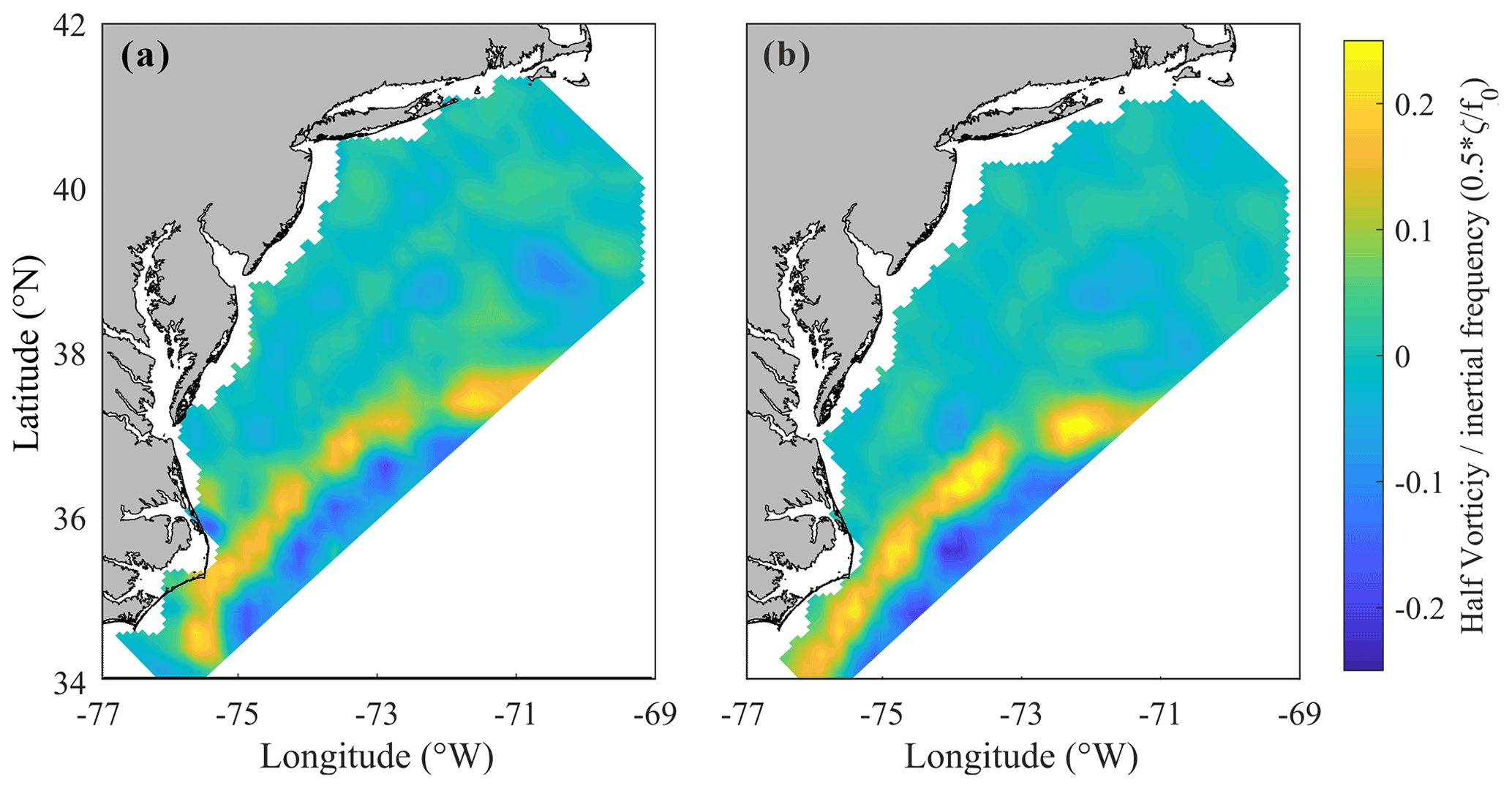
Figure 10 Spatial distribution of background vorticity (a) before the hurricane event on 25 August and (b) after the hurricane event on 4 September.

4.3 Decay timescale of NIKE

It is of practical importance to determine the rate of NIKE decay. A conventional measure of the rate of NIKE may be its e-folding time, i.e., the timescale in which the NIKE decreases by a factor of e. Shown in Fig. 11 is the e-folding time of the depth-integrated NIKE at 24 stations along sections A to D. The decay timescale in section E is not considered because this section is relatively far from the hurricane track compared with other sections and also because the orientation of section E differs quite significantly from that of other sections.

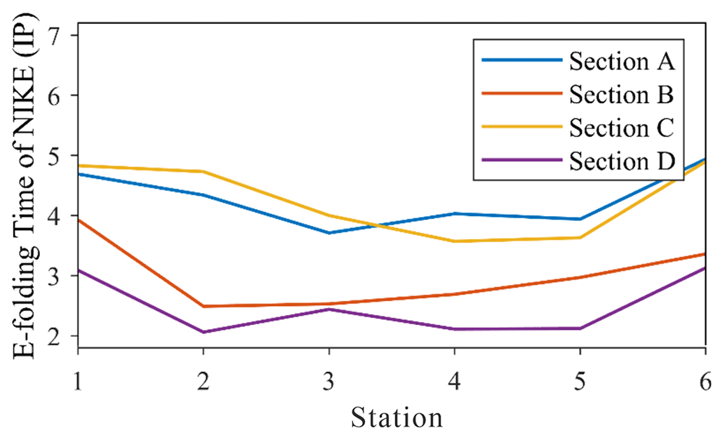
Figure 11 The decay timescale of the depth-integrated NIKE at 24 stations along sections A to D. Note that the unit for the e-folding time is the inertial period.

It is interesting to note that the decay timescales in the shallow and deep regions are fairly different. As shown in Fig. 11, NIKE is dissipated much more slowly outside the shelf break (station no. 6) than over the continental shelf. This difference is often considered to be an effect of the bottom friction and the extremely strong turbulence in the shallow waters, as pointed out by other researchers (Rayson et al., 2015; Shen et al., 2017). It is also interesting to find that the variation of the NIKE decay rate in shallow waters is much more complicated than in deep waters. In the cross-shore direction, the NIKE at the middle stations, i.e., station no. 3 to no. 5 located at the outer half of the continental shelf, is shown to be dissipated most rapidly, especially along sections A to C (Fig. 11). This phenomenon is actually supported by the fact that the strongest turbulence diffusion occurred over the outer half of the continental shelf, particularly in the relevant region between sections A and C (Fig. 9a). Considering that the variation of the wind energy input within the same section should not be too large, the ratio of turbulence diffusion to wind energy input must be mainly determined by the turbulence diffusion. Therefore, the strong turbulence dissipation due to the strong vertical shear in well-maintained stratification is responsible for the rapid energy decay in the outer half of the continental shelf, as shown in Sect. 4.2. Although the bottom friction also has some effect on the decay timescale of NIKE onshore, the turbulence effect is predominant.

In the alongshore direction, it is shown that the NIKE in sections B and D decayed more rapidly. Actually, the decay timescale there is only two to three inertial periods compared to four to five inertial periods in sections A and C. However, the limited variability of the turbulence diffusion in the alongshore direction should not lead to such a big difference. Near section A, the vorticity ridge in the Gulf Stream restricted the lateral divergence of NIKE, which may contribute to a long decay timescale to some extent. However, the role of this effect was limited. In fact, as mentioned in Sect. 3, the nonlinear wave–wave interaction near section B may have caused a transfer of NIKE to other frequencies, as also pointed out by Shen et al. (2017). In fact, it is found that the ratio of turbulence diffusion to wind input in section B was larger than in other sections by 20 %–30 % due to the low level of wind input (Fig. 8b) and high level of turbulence dissipation (Fig. 9a) there. These factors combined seem to have yielded an extraordinarily short e-folding time in section B. In section D, due to the complete destruction of stratification after the hurricane event (as mentioned in Sect. 3 and shown in Fig. 7d), the NICs were of the same order as the background flow (D1–D4 in Fig. 6). Therefore, the decay timescale of NIKE in section D is certainly inaccurate and possibly meaningless.

5 Conclusion

This study aimed to investigate the development and decay mechanism of NICs in the MAB area caused by Hurricane Irene (2011). Numerical results obtained with ROMS are shown to agree well with the observational data. Both computational and observational results show that the rotating wind of the hurricane immediately forced a rotating current in the surface layer of the ocean and induced an inertial current rotating in the opposite direction about one inertial period after the hurricane passed over. The NICs overwhelmed the M2 tide in most areas of the MAB region except in the nearshore area where the stratification was totally destroyed by the strong mixing due to turbulence. In addition, the cross-shore component of the NIC velocity gradually increases by a factor of at least 3 from a shallow-water position to the shelf break.

The energy budget in the NICs is investigated in both deep and shallow waters. NIKE was shown to be immediately gained from the wind power during the hurricane event. In the deepwater region, NIKE was mainly dissipated by the vertical diffusion due to turbulence and partially transferred to deep waters. In the continental shelf region, NIKE was basically dissipated by the turbulence diffusion. Meanwhile, the bottom friction played a secondary role. The nonlinear wave–wave interaction only dissipated NIKE in limited regions, e.g., shelf waters off the Delmarva Peninsula. Notably, the lateral divergence of NIKE should be taken into consideration in both shallow-water and deepwater regions under hurricane conditions. However, in the southern MAB, it was restricted by a vorticity ridge at the edge of the Gulf Stream. It is also clarified that the NIKE dissipation due to turbulence diffusion is much more closely related to the rate of vertical shear than the intensity of turbulence, which certainly takes place in a region where wind energy input achieves a high level. The strong vertical shear at the offshore side of the continental shelf led to the strong turbulence dissipation in this region.