the Creative Commons Attribution 4.0 License.
the Creative Commons Attribution 4.0 License.
 | 05 Oct 2022
Major sources of North Atlantic Deep Water in the subpolar North Atlantic from Lagrangian analyses in an eddy-rich ocean model
Patricia V. K. Handmann
Arne Biastoch
The North Atlantic Deep Water (NADW) is a crucial component of the Atlantic meridional overturning circulation and is therefore an important factor of the climate system. In order to estimate the mean relative contributions, sources, and pathways of the NADW at the southern exit of the Labrador Sea, a Lagrangian particle experiment is performed. The particles were seeded according to the strength of the velocity field along the 53∘ N section and traced 40 years backward in time in the three-dimensional velocity and hydrography field. The resulting transport pathways, their sources and corresponding transit timescales were inferred. Our experiment shows that, of the 30.1 Sv of NADW passing 53∘ N on average, the majority of this water is associated with a diapycnal mass flux without contact to the atmosphere, accounting for 14.3 Sv (48 %), where 6.2 Sv originate from the Labrador Sea, compared to 4.7 Sv from the Irminger Sea. The second-largest contribution originates from the mixed layer with 7.2 Sv (24 %), where the Labrador Sea contribution (5.9 Sv) dominates over the Irminger Sea contribution (1.0 Sv). Another 5.7 Sv (19 %) of NADW crosses the Greenland–Scotland Ridge within the NADW density class, where about two-thirds pass the Denmark Strait, while one-third crosses the Iceland–Scotland Ridge. The NADW exported at 53∘ N is hence dominated by entrainment through the diapycnal mass flux and mixed-layer origin in the Labrador Sea.
- Article
(5502 KB) - Full-text XML
-
Supplement
(7432 KB) - BibTeX
- EndNote


The meridional overturning circulation (MOC) is the global redistribution system of heat, mass, fresh water, and tracers. Water mass transformation from the upper to the lower MOC component associated with deep convective mixing (Lab Sea Group, 1998; Marshall and Schott, 1999) and diapycnal mixing (Straneo, 2006; Katsman et al., 2018; Johnson et al., 2019) occurs in only a few key regions globally, one of them being the highly complex region of the subpolar North Atlantic (SPNA). The associated density increase eventually results in a net downwelling of upper Atlantic MOC (AMOC) water in density space (Johnson et al., 2019) and thereby the formation of deep and intermediate water (Rhein et al., 2011). These water masses are then transported southward through the Deep Western Boundary Current (DWBC), (Dickson and Brown, 1994; Molinari et al., 1998) as well as the interior, as part of the deep AMOC branch (Bower et al., 2009). Water mass properties of the North Atlantic Deep Water (NADW) are largely imprinted within the SPNA and the Nordic Seas and are mostly maintained farther south (Haine et al., 2008).
In observations at 53∘ N, i.e., the southern exit of the Labrador Sea, all three components of the NADW are present in the DWBC. The shallowest component, named Labrador Sea Water (LSW), is thought to be majorly formed through deep convective mixing in the Labrador Sea (Yashayaev and Loder, 2016). This water mass is regularly ventilated in winter and is defined as a low potential vorticity water mass with conservative temperatures below 4 ∘C and densities between 27.70–28.10 kg m−3 in neutral density (γn), 27.68–27.80 kg m−3 in potential density (σ0) (e.g., Pickart et al., 1997; Stramma et al., 2004; Mertens et al., 2014; Liu and Tanhua, 2021), and 36.50–36.94 kg m−3 in potential density relative to 2000 m (σ2) (e.g., van Sebille et al., 2011; Zantopp et al., 2017). The first lower NADW (lNADW) component is the Northeast Atlantic Deep Water (NEADW) which is modified Iceland–Scotland Overflow Water (ISOW) originating at the overflows of the Iceland–Scotland Ridge (ISR) that was modified along its spreading pathway. This water mass features conservative temperatures between 2.2–3.3 ∘C and high absolute salinities of >34.95 g kg−1, with γn between 28.00–28.15, σ0 between 27.80–27.88 kg m−3, and σ2 between 36.94–36.98 kg m−3 (Hansen and Østerhus, 2000; Østerhus et al., 2001; Jochumsen et al., 2015). NEADW appears as a salinity maximum at depth in the hydrography of 53∘ N below the LSW component. The deepest lNADW component is the Denmark Strait Overflow Water (DSOW) originating at the overflow sills of the Denmark Strait (DS) between Greenland and Iceland, with densities of γn>28.15 kg m−3, σ0>27.88 kg m−3, and σ2>36.98 kg m−3 (Pickart et al., 1997; Schott et al., 2006; Liu and Tanhua, 2021). NEADW and DSOW are modified through entrainment of upper-ocean water after passing the Greenland–Scotland Ridge (GSR) and descending into the SPNA (Fogelqvist et al., 2003; Chafik et al., 2020).
From the observed mid-depth flow field (Palter et al., 2016; Fischer et al., 2018), the spreading path of the mid-depth water masses is known as follows: the ISOW flows along the eastern flank of the Reykjanes Ridge after crossing the ISR and entering the Iceland Basin from the Nordic Seas. Two paths, through the Charlie–Gibbs Fracture Zone (CGFZ) and the Bight Fracture Zone (Lankhorst and Zenk, 2006; Zou and Lozier, 2016; Xu et al., 2018), connect the Iceland and Irminger basins passing the Mid-Atlantic Ridge. More recent model-based studies reveal an additional westward branch from the Iceland Basin through the Reykjanes Ridge and crossing through the interior Irminger Sea towards the Labrador Sea (Xu et al., 2010; Zou et al., 2020a). The mean mid-depth circulation shows a confined current band west of the Reykjanes Ridge towards the DS. South of the DS it encounters the DSOW (Pickart, 1992; Dickson and Brown, 1994) and is transported farther south around Greenland and the Labrador Sea basin through the DWBC. A confined boundary current is established along the East Greenland shelf break. Once the western boundary current (WBC) passes Cape Farewell (while being partly dispersed), the WBC refocuses along the West Greenland shelf break. At Cape Desolation, where eddies are shed towards the interior Labrador Sea (Hátún et al., 2007; Prater, 2002; Lilly et al., 2003; Rieck et al., 2018), the WBC is partly dispersed, and just north of it a bifurcation of the boundary current, following the 1500 and 3000 m isobaths of the northwestern Labrador Sea, takes place (Cuny et al., 2002; Higginson et al., 2011; Palter et al., 2016; Fischer et al., 2018). At the coast of Labrador, the flow becomes confined in the boundary current again.
The importance of Labrador Sea convection for the strength and the variability of the AMOC still remains unclear and is currently under debate (Lozier, 2012; Rhein et al., 2013; Yeager et al., 2021). While some studies assume a direct linkage (Marshall and Schott, 1999; Yashayaev et al., 2008; Haine et al., 2008), others corroborate the assumption that the AMOC is only minimally impacted by Labrador Sea convection (Pickart and Spall, 2007; Zou and Lozier, 2016; Lozier et al., 2019; Petit et al., 2020). Deep convective mixing has been widely observed since the 1950s (Dietrich, 1957; Lazier, 1973) in the Labrador Sea, and there is an increasing amount of observations of deep convection south of Cape Farewell and in the Irminger Sea (see Rühs et al., 2021, for an extensive literature collection). The interest in understanding exactly where the transformation from upper AMOC water to lower AMOC water takes place in the SPNA has increased in recent years. Several studies, within medium- to high-resolution ocean models, have shown that, in addition to deep convective mixing, diapycnal mixing between the basin interior and the boundary currents and densification along the spreading pathways at the boundary currents play a crucial role for the total formation of dense deep water (e.g., Straneo, 2006; Katsman et al., 2018; Desbruyères et al., 2019; Sayol et al., 2019; Georgiou et al., 2020; Petit et al., 2020). The extent of the relative importance of these sources and their respective pathways for the total deep-water export towards the south and its variability is not completely clear yet.
Newer research has shown that a major volume of water is transformed along the North Atlantic Current path (Desbruyères et al., 2019). This water originates from different transformation processes, which are related to different export timescales (Le Bras et al., 2020). Hence, the very localized deep convection might only be adding a comparatively small amount of transformed water to the overall NADW volume. Additionally, the observed deep convection in the Irminger Sea increased over the past years (Våge et al., 2009; de Jong et al., 2012; Jong and Steur, 2016; Piron et al., 2016; Fröb et al., 2016; de Jong et al., 2018; Rühs et al., 2021). In contrast to the well-documented southward spreading of deep water south of 45∘ N from the subpolar gyre, the dynamics of the formation and subsequent spreading of NADW within the SPNA are not so well documented nor understood. In this model-based study, we present (i) the relative contributions of the respective deep-water sources to the NADW transport at 53∘ N and (ii) the pathways and advection timescales of the connections between 53∘ N and the respective deep-water sources. The methods and model used to perform the desired analyses are presented in Sect. 2. Subsequently, we present the sources and pathways of each deep-water particle category in Sect. 3.1. In Sect. 3.2, the water mass properties of the different water masses are presented. To conclude and classify the results within the current literature, the results are then discussed in Sect. 4, and our conclusions close this paper in Sect. 5.
2.1 Lagrangian experiment in VIKING20X-JRA-OMIP
The model output used to conduct our Lagrangian experiment is the eddy-rich nested ocean–sea-ice model configuration VIKING20X-JRA-OMIP, which (as the name reveals) is forced by the JRA55 forcing and covers the period from 1958 to 2019 (version 1.4, Tsujino et al., 2018); see Biastoch et al. (2021) for a full model description of VIKING20X and the experiment used here. It is based on the global ∘ resolution grid of the Nucleus for European Modelling of the Ocean code (NEMO, version 3.6, Madec et al., 2017) and the Louvain la Neuve Ice Model (LIM2, Fichefet and Maqueda, 1997). The tripolar ∘ global horizontal grid is refined in the Atlantic Ocean to ∘, yielding an effective grid spacing of ≤5 km in the SPNA. It contains 46 geopotential z levels, increasing in thickness from ∼6 m at the surface to ∼250 m in the deepest layers. Here, daily snapshots of the three-dimensional Eulerian flow and hydrographic fields are used for the offline Lagrangian particle tracking experiment. Biastoch et al. (2021) show that the model reproduces both the major and regional dynamic properties in the SPNA region, such as the strength and width of the boundary currents; the position, depth, and expansion of the mixed layer (see also Rühs et al., 2021); and an AMOC strength comparable to observations. To conduct the offline Lagrangian particle experiment, the Python module Parcels (version 2.2.2, Delandmeter and Sebille, 2019) is utilized. Trajectories are estimated by advecting virtual particles along streamlines that are calculated from the Eulerian flow field. We hence analyze the output of the ocean model in detail through the Lagrangian particle experiment.
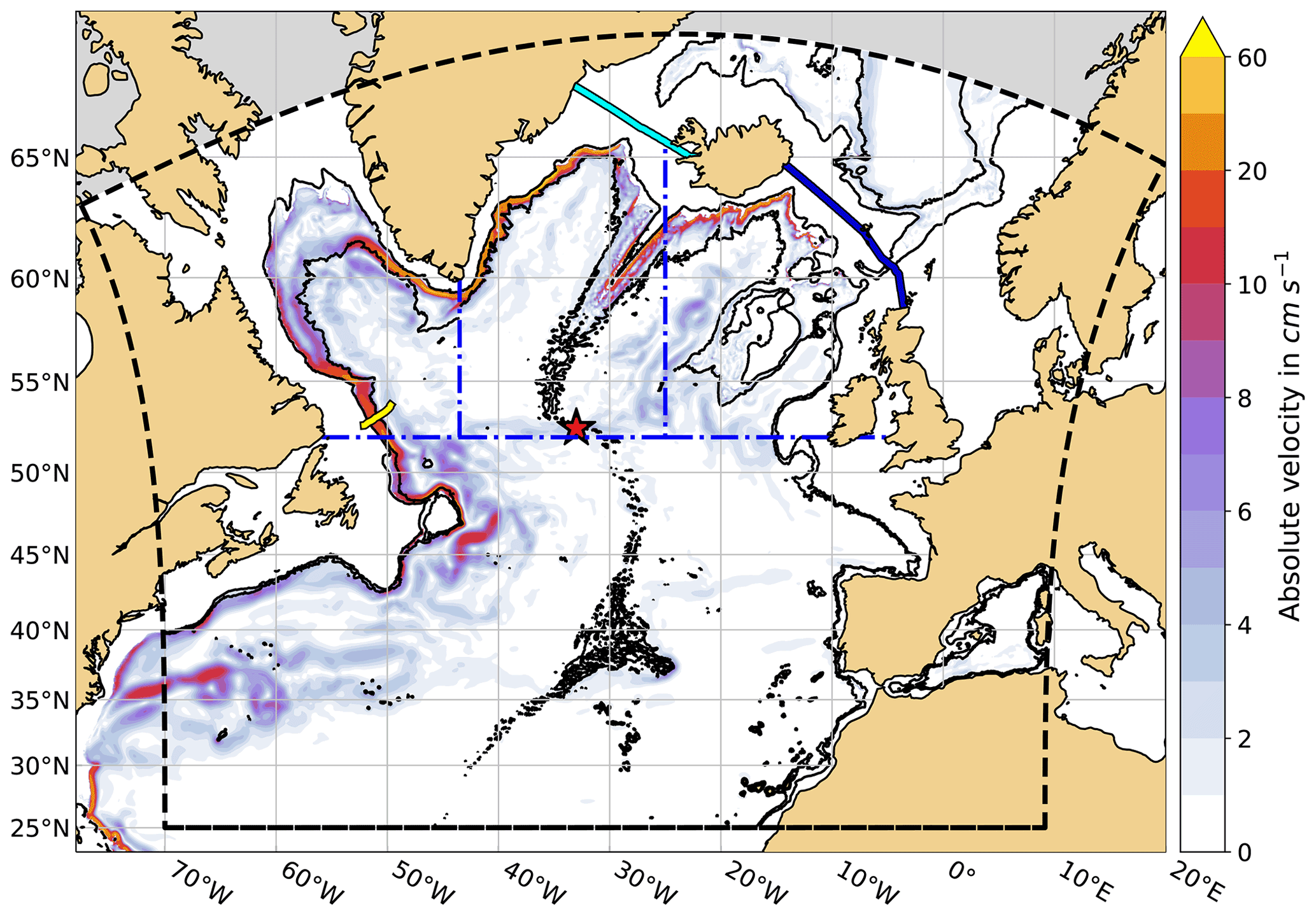
Figure 1Mean absolute velocity (1958–2019, in cm s−1, shading) at 1298 m in VIKING20X-JRA-OMIP. The Charlie–Gibbs Fracture Zone is indicated by the red star. The yellow line marks the 53∘ N section, and the light and dark blue lines mark the Denmark Strait and Iceland–Scotland Ridge sections, respectively. The dashed black line indicates the boundary of the experiment domain considered in this study. The dashed–dotted blue lines indicate the areas that are used to calculate the Labrador Sea (west of 43.5∘ W; north of 52∘ N), the Irminger Sea (43.5 to 25∘ W; north of 52∘ N, south of the GSR), the Iceland Basin (east of 25∘ W; north of 52∘ N, south of the GSR) and southern SPNA (south of 52∘ N) volume transport contributions. The black contours indicate the 1000 and 3000 m isobaths, respectively, in the Labrador Sea area, as indicated by the dashed–dotted blue lines. In the remaining SPNA the black contours indicate the 1000 and 2000 m isobaths, respectively.
The domain in which the Lagrangian particle experiment is conducted is bounded to the north by the northern boundary of the high-resolution nest of VIKING20X (the northernmost point is 69.3∘ N) and by 25∘ N to the south. The easternmost point is 20∘ E, while the westernmost point is 77.5∘ W. However, due to the tripolar grid of the model, the exact northern, eastern, and western boundaries of the domain vary (see dashed black line in Fig. 1).
2.1.1 Seeding strategy
Virtual particles are released at a section along the observational mooring array at 53∘ N (Zantopp et al., 2017) off the coast of Newfoundland (yellow line in Fig. 1), which is part of the Overturning in the subpolar North Atlantic Program (OSNAP, Lozier et al., 2017, 2019). The section in the model is approximated following the tripolar model grid in the x and y directions (Handmann, 2019, chapter 4.3). Virtual particles are released daily during the period 2010 through 2019 in each grid box along this section. Following Schmidt et al. (2021), the amount of particles released in each grid box is defined relative to the volume transport associated with each individual grid box. If Vgb is the volume transport of a given grid box and Vth>0 a volume transport threshold determining the maximum absolute volume transport assigned to an individual particle, then the number of particles Ngb released within the given grid box is defined by
where ⌈⌉ is the ceiling function. The volume transport assigned to each particle Pi within a grid box is then defined as
where i=1…Ngb. Subsequently, particles are only released in grid boxes where |Vgb|>0. For grid boxes where , only one particle is released, which is assigned exactly the absolute transport value that is associated with the corresponding grid box. If |Vgb|>Vth, the transport associated with the given grid box is distributed equally among multiple particles Pi. Thus, each particle is associated with a predefined volume transport value that varies among particles from different grid boxes.
The release positions of the individual particles are determined by randomly distributing the particles across their corresponding grid box. Since this study is concerned with the NADW export from the Labrador Sea, particles are only released in a southeast-directed flow. Particles are seeded throughout the entire water column with a maximum volume transport per particle of 0.1 Sv. This results in a total of approximately 8.9×10⁶ particles being released.
2.1.2 Experiment execution
The virtual particles are integrated backwards in time for 14 600 d (∼40 years) using a fourth-order Runge–Kutta scheme at a time step of 5 min. Since no additional diffusion kernel is applied, the obtained particle trajectories are equivalent to volume transport pathways (Schmidt et al., 2021). An additional kernel is however incorporated to sample potential temperature, salinity, and mixed-layer depth along the particles' trajectories. Note that Parcels assumes tracer values to be constant within individual grid boxes for Arakawa C-type grids (Delandmeter and Sebille, 2019). The particle positions and properties are stored at daily resolution.
2.1.3 Categorization of particles
Here we focus on NADW; hence, only particles released within this water mass are considered during the analyses. All particles lighter than the upper NADW boundary at the seeding location are filtered out and not considered hereafter. The upper boundary of NADW is the density of the AMOC maximum at OSNAP, in VIKING20X-JRA-OMIP defined as kg m−3 (Biastoch et al., 2021). To start with, the LSW was defined as 27.62 kg m kg m−3. Consequently, the lNADW in the model is found at σ0≥27.86 kg m−3 (Handmann et al., 2018; Biastoch et al., 2021). The water mass boundaries are defined as the mean density value over the complete model output, covering 1958 through 2019. Contrary to the dynamically defined upper bound of NADW, the definition of the boundary between LSW and lNADW is based on the hydrography in the central Labrador Sea (Handmann et al., 2018). Even though this method works fine with observations and yields the distinct densities of the three NADW water masses, we show in this study that this does not necessarily hold for a water mass distinction in the classical sense in an ocean model. This is partly related to the unrealistically large diapycnal mixing in regions where dense waters descend topographic slopes, producing lighter water (Willebrand et al., 2001). This spurious mixing is dependent on the vertical and horizontal resolution of the ocean model and is a typical model artifact. It is also a reason why we did not define the density boundary between NEADW and DSOW (Handmann et al., 2018) here, which is additionally difficult due to changes in water mass properties along the spreading pathways of NEADW.
The particles are subsampled based on their density at their respective release, i.e., only particles released at densities σ0≥σDW are considered, resulting in a subset of particles. These particles are referred to as NADWP, amounting to approximately 3.5×10⁶ particles. Once the particles belonging to the NADW water mass are identified, they are then divided into five mutually exclusive categories. The categories are defined based on the particles' point of origin. For each particle, the trajectory is considered only between the particle's origin, described in detail in the following, and 53∘ N. Resulting from the definition of the point of origin, the trajectories have varying lengths. In turn, these are consequently related to varying transit times. However, all resulting trajectories lie entirely within the NADW density range and within the North Atlantic. The terms source, origin, and point of origin are used synonymously in this work. Note that despite being calculated backwards in time, the trajectories are referred to in their forward sense in the following, i.e., in flow direction. Consequently, the particle release at 53∘ N constitutes the last time step or the end of the trajectory. Hence, the point of origin is considered the first time step.
In short, each particle trajectory has a defined point of origin or source. This point of origin is defined as the point where a particle changes its density from σ0<σDW to σ0≥σDW or where it last crosses a defined section with a density σ0≥σDW.
Particles that cross the Greenland–Scotland Ridge (GSR) and retain densities of σ0≥σDW represent NADW crossing the GSR from the Nordic Seas into the SPNA. The section that particles need to cross in order to be taken into account here is a combination of two subsections, the DS and the ISR. The particles are classified as DSP or ISRP depending on the section they cross. The subsections are extracted from the model grid as described in Handmann (2019, chapter 4.3). In Fig. 1, the two sections are indicated by the solid light and dark blue lines, respectively. For DSP and ISRP, the point of origin is the last crossing of the GSR within the NADW density before reaching 53∘ N. The particle information along the respective trajectories is only considered between the last crossing of the GSR and arriving at 53∘ N. Therefore, parts of the trajectories lying within the Nordic Seas or recirculating over the GSR are not considered, as we do not consider the density change north of this section. As all NADW is considered, we call these particle categories “overflow water” in the following as they are NADW flowing over the sills; however, these two particle categories do not necessarily resemble the overflow water masses from observations.
If particles increase their density during the experiment from σ0<σDW to σ0≥σDW outside of the mixed layer before reaching 53∘ N and without contact to the atmosphere, this is referred to as diapycnal mass flux, and the particles are classified as DIAP. If this threshold is not met and the respective density increase occurs within the mixed layer with contact to the atmosphere, the particles are classified as MLP. The pivotal density change of a particle is the last increase from σ0<σDW to σ0≥σDW before reaching 53∘ N. Hence, the exact processes and property changes in the mixed layer are not explicitly considered here. To separate DIAP from MLP the particle depth is compared to the instantaneous mixed-layer depth at the particle position, which is stored during the experiment along each particle's trajectory (Sect. 2.1.2). For DIAP, trajectories are only considered between the point of respective density increase and reaching 53∘ N, i.e., the point of origin is defined as the point of density transition from the upper AMOC component to the NADW below the mixed layer. For MLP, trajectories are considered between leaving the mixed layer and arriving at 53∘ N, i.e., the point of origin is the location where the particles leave the mixed layer, after having changed their density from the upper AMOC to NADW density within the mixed layer.
The particles that can not be assigned to any of the previous categories form the last category. Particles belonging to this category retain densities σ0≥σDW throughout their entire advection time and are referred to as RESP. These particles either reside within the North Atlantic during the whole experiment or enter the domain at any point in time through its lateral boundaries (except through the GSR). Particles of this category do not have a defined point of origin.
It is important to point out that every particle belonging to any of the described categories can still be entrained into the mixed layer. These mixed-layer contacts, however, are not associated with a densification from σ0<σDW to σ0≥σDW.
In order to differentiate the region of densification, the particle categories are further divided by their position above topography. Since in the SPNA the boundary current sticks to the strong shelf break, the particle is classified as being in the boundary if the underlying bathymetry is shallower than 3000 m in the Labrador Sea or 2000 m in the remaining SPNA (Fig. 1). If the bathymetry is deeper, the density transition is located in the basin interior.
2.2 Analyses
In the following, all volume transport estimates are given with respect to the 10-year mean NADW volume transport at 53∘ N of 30.1 Sv from 2010 to 2019. First, particles are grouped based on a certain condition (e.g., point of origin). Then, the cumulative transport of all particles within a group is divided by the cumulative transport of all NADWP. The obtained fraction is then multiplied by the mean transport at 53∘ N to obtain the mean volume transport associated with the defined particle group.
To derive the relative and absolute transport contributions of the different volume transport sources, the particles are separated into five categories, as described in Sect. 2.1.3. The corresponding contributions are then estimated as explained above.
In order to compute the transport distribution at 53∘ N, particles are grouped into 5 km × 0.01 kg m−3 bins, where the distance refers to the horizontal distance from the starting point of the section. To obtain a depth profile, the transport is then summed over all distance bins and two density bins each, resulting in 0.02 kg m−3 bins.
To evaluate the horizontal pathways of the particles, we follow Sect. 4.3 in van Sebille et al. (2017). A regular latitude–longitude grid is defined. For each grid cell the transport-weighted number of particles visiting the grid cell is estimated, which is independent of the respective flow direction through the grid cell. Each particle, however, is only accounted for once per grid cell (recirculation is not considered). By dividing the resulting cumulative transport per grid cell by the total transport of all NADWP, transport-weighted probability maps are derived. These reflect the pathways in the horizontal plane that are associated with most of the volume transport conducted by the particles. In other words, the transport-weighted fraction of particles visiting a certain grid cell at least once is obtained. Within each grid cell values can range between 0 and 1 or 0 % and 100 %, equivalently. This would be the case if none (0 %) or all (100 %) of the particles pass through the same grid cell. In the following, grid cells with values <0.01 % are masked out.
Since, by definition, the source of DSP and ISRP is known, the point of origin is only binned for MLP and DIAP. A regular latitude–longitude grid is defined, and for each grid cell the transport-weighted number of particles, whose point of origin is located within the particular grid cell, is obtained. Therefore, integrating the transport over all grid cells yields the volume transport at 53∘ N associated with DIAP and MLP. The resulting maps can then be used to identify regions from which most of the NADW volume transport originates. Grid cells with values Sv are masked out. To determine the transport contributions of different ocean basins, the SPNA is divided into four distinct areas. These areas are indicated by the dashed–dotted blue lines in Fig. 1. Integrating the transport over all grid cells within each of these defined areas yields the transport associated with the respective basin. The different regions are denoted Labrador Sea, Irminger Sea, Iceland basin, and southern SPNA in the following.
For each particle the transit time, i.e., the time it takes a particle, starting from its respective point of origin, to reach 53∘ N is calculated. The particles are then binned based on their transit times into 1 month bins. The transport per bin is estimated as described above. Additionally, the transport is summed over all bins, cumulatively.
To obtain the volumetric water mass transformations, the particles are grouped by their water mass properties at 53∘ N and at their point of origin. The considered properties are σ0, absolute salinity (SA), and conservative temperature (Θ), with bin sizes of 0.025 kg m−3, 0.01 g kg−1, and 0.2 ∘C, respectively. These properties were computed from the practical salinity, potential temperature, and depth tracked along each trajectory using the TEOS-10 toolbox for Python (Intergovernmental Oceanographic Commission, 2015). The difference between the volume at 53∘ N and the volume at the point of origin for the σ0, SA, and Θ classes then gives the volumetric water mass transformation.
To evaluate the evolution of the particle properties along the individual pathways, the maximum or minimum salinity and temperature are determined along a particle trajectory. Then, the location along the trajectory is determined where the difference in salinity or temperature between the extremum and the particle source is halved. Based on these locations, the particles are then grouped into longitude–latitude bins and the transport-weighted mean particle depth per bin is estimated.
3.1 Sources, pathways, and transit timescales
Here we start with a general assessment of the absolute and relative transport contributions of the defined particle categories (Sect. 2.1.3, Fig. 1) and a description of the transport distributions (Fig. 2). Common features of the particle pathways (Fig. 3) are introduced as well. This is followed by a detailed evaluation of the origin locations (Fig. 4) and their relative importance (Table 2), the spreading pathways (Fig. 3), and the associated transit timescales (Fig. 5) for each particle category, ordered by the relative contribution to the transport at 53∘ N.
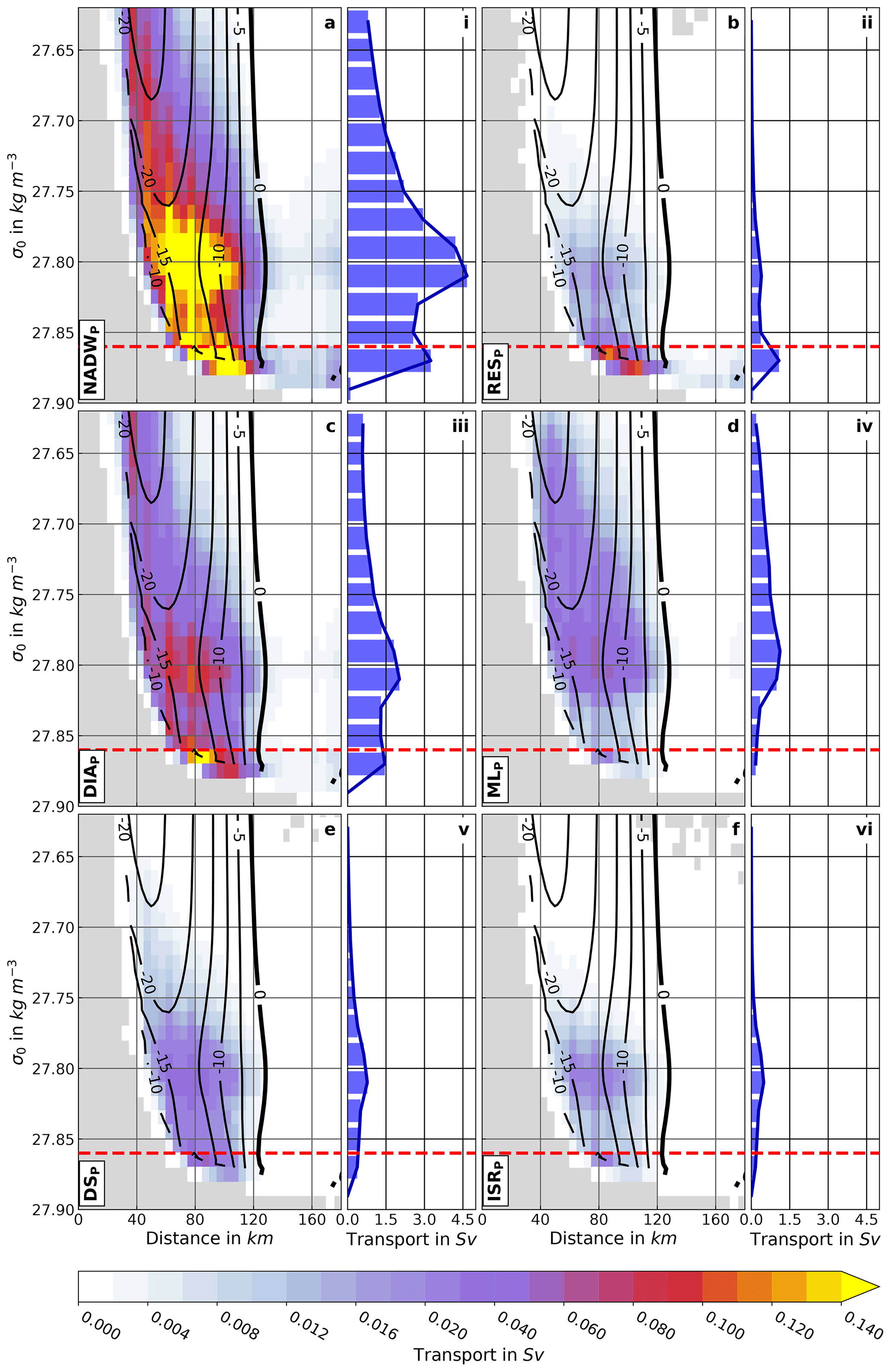
Figure 2Mean transport distribution at 53∘ N (in Sv) in density space (a to f, shading, 5 km × 0.01 kg m−3 distance–density bins) and mean transport accumulated along 53∘ N (in Sv) (i) to (vi), 0.02 kg m−3 bins). The dashed red lines mark the mean σ0=27.86 kg m−3 isopycnal. Black contours in (a) to (f) are mean meridional velocities (in cm s−1). Note the nonlinear color scale (0.002 Sv intervals up to 0.02 and 0.01 Sv intervals starting from 0.02 Sv) for (a) to (f). Mean transport distributions are shown for (a, i) NADWP, (b, ii) RESP, (c, iii) DIAP, (d, iv) MLP, (e, v) DSP, and (f, vi) ISRP (see Sect. 2.1.3 for details of the definitions).
Table 1Mean transport from 2010–2019 (in Sv) at 53∘ N associated with each particle category (DIAP, MLP, DSP, ISRP, and RESP), as detailed in Sect. 2.1.3, as well as their relative contributions (in %) for σ0≥27.62 kg m−3 (NADW), kg m−3 (LSW), and σ0≥27.86 kg m−3 (lNADW). The transports are rounded to 0.1 Sv.
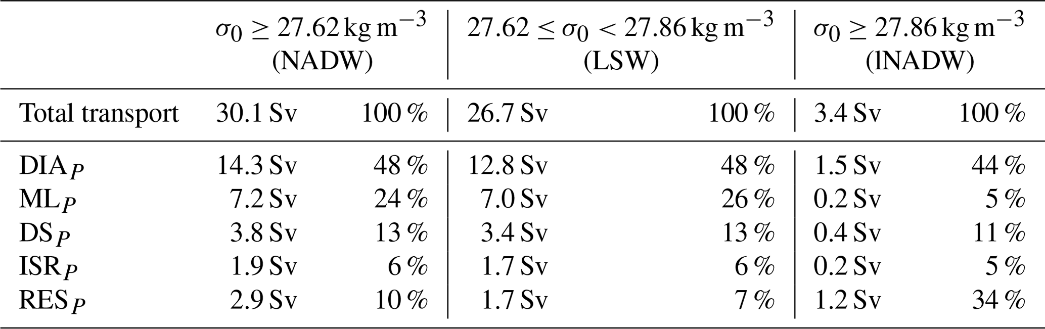
The mean southward NADW transport in the presented Lagrangian experiment (Fig. 2a, i) shows two peaks in density space, the first of which is located around σ0=27.80 kg m−3. A secondary peak is found around σ0=27.87 kg m−3 (Fig. 2i). The upper, lighter transport peak is associated with transport peaks around 27.80 kg m−3 for all four defined particle sources (Fig. 2iii–vi). The dense maximum (Fig. 2i), on the other hand, is dominated by DIAP and RESP (Fig. 2ii–iii). Diapycnal mass flux dominates the transport distribution throughout the water column with an overall mean transport of 14.3 Sv (48 %, Table 1 and Fig. 2). In the density range kg m−3, DIAP amounts to 12.8 Sv (48 %), with the second-largest contributor being particles from the mixed layer (7.0 Sv or 26 %, Table 1). The component with densities σ0≥27.86 kg m−3 (below the dashed red line in Fig. 2) is dominated by DIAP, with 1.5 Sv (44 %), while the second-largest contribution, 1.2 Sv (34 %), is associated with RESP (Table 1). Overall, DSP contributes 3.8 Sv (13 %) to the southward NADW transport at 53∘ N, with about 3.4 Sv (13 %) within the density range of kg m−3 and 0.4 Sv (11 %) at densities σ0≥27.86 kg m−3. ISRP amounts to 1.9 Sv (6 %) throughout the NADW σ0 range, with 1.7 Sv (6 %) for the density range kg m−3 and 0.2 Sv (5 %) at densities σ0≥27.86 kg m−3 (Table 1).
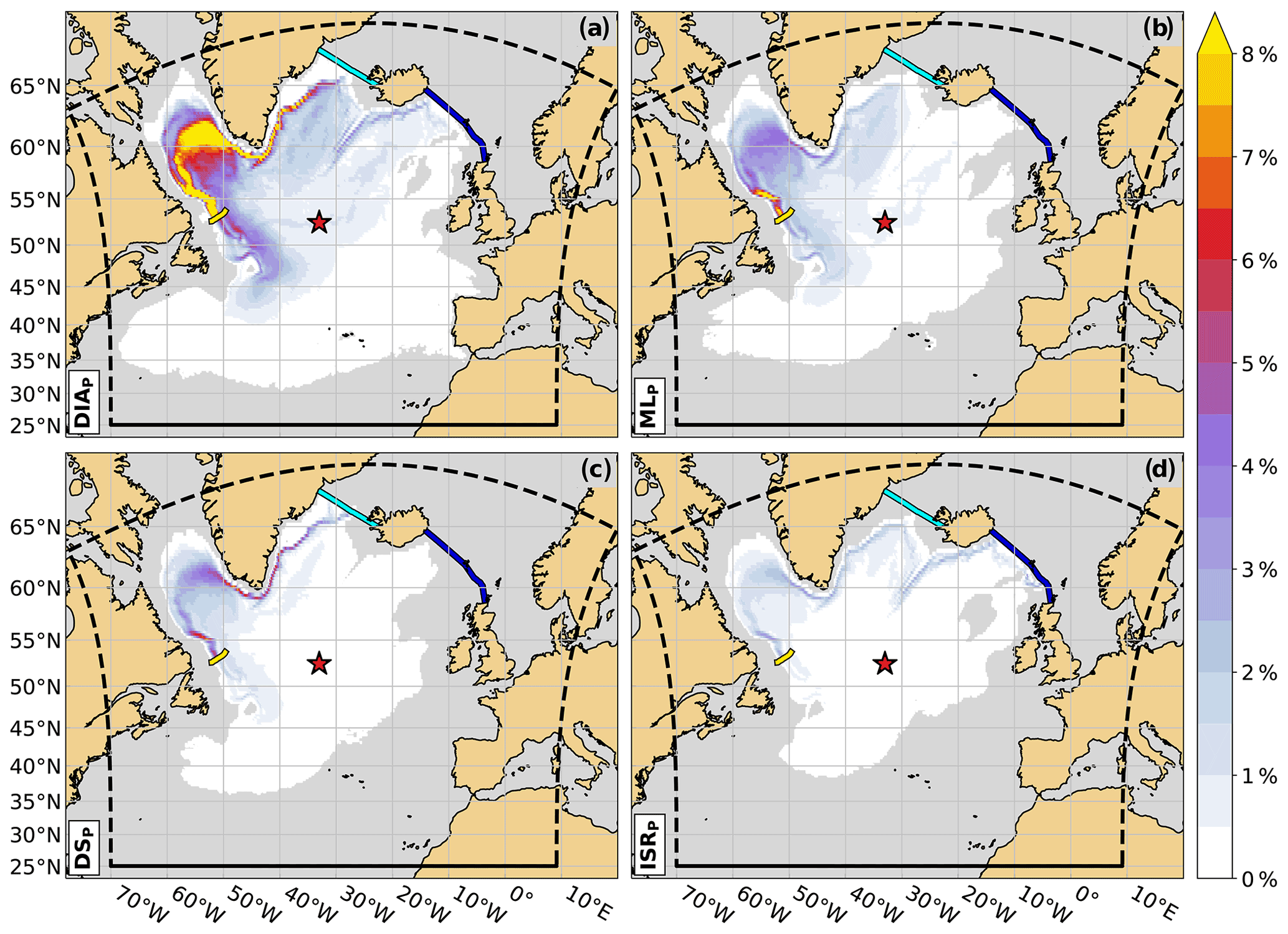
Figure 3Particle pathways associated with most of the volume transport, calculated as transport-weighted probability density maps (∘ bins) of the different particle categories: (a) DIAP, (b) MLP, (c) DSP, and (d) ISRP (see Sect. 2.1.3 for details of the definitions). The Charlie–Gibbs Fracture Zone is indicated by the red star. The yellow line marks the 53∘ N section, and the light and dark blue lines mark the Denmark Strait and Iceland–Scotland Ridge sections, respectively. The dashed black line indicates the boundary of the experiment domain.
The main spreading pathways from the respective sources to 53∘ N (Fig. 3) are largely concentrated within the boundary currents for all four particle categories. In the northeastern Labrador Sea, near Cape Desolation (west of Greenland), the pathways fan out for all categories, most probably related to the eddy activity here (Rieck et al., 2018), namely the shedding of Irminger rings. Furthermore, all particle categories exhibit pathways extending southward from 53∘ N (Fig. 3). These pathways become more distinct on longer timescales and represent the recirculation south of 53∘ N at the Orphan Knoll region (not shown).
Table 2Mean transport contributions (2010–2019) from the Labrador Sea (LS) and Irminger Sea (IS), the Iceland basin, as well as the remaining SPNA south of 52∘ N (southern SPNA) in Sv. The regions are outlined by the dashed–dotted blue lines in Fig. 1. The Labrador and Irminger Sea contributions are separated into an interior and boundary component (water depths shallower than 3000 m in the Labrador Sea and 2000 m elsewhere). Transport contributions are given for DIAP and MLP (see Sect. 2.1.3 for details of the definitions). Values are given for σ0≥27.62 kg m−3 (NADW) and kg m−3 (LSW); the difference between the two corresponds to the transport associated with σ0≥27.86 kg m−3 (lNADW).
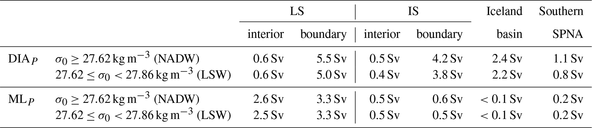
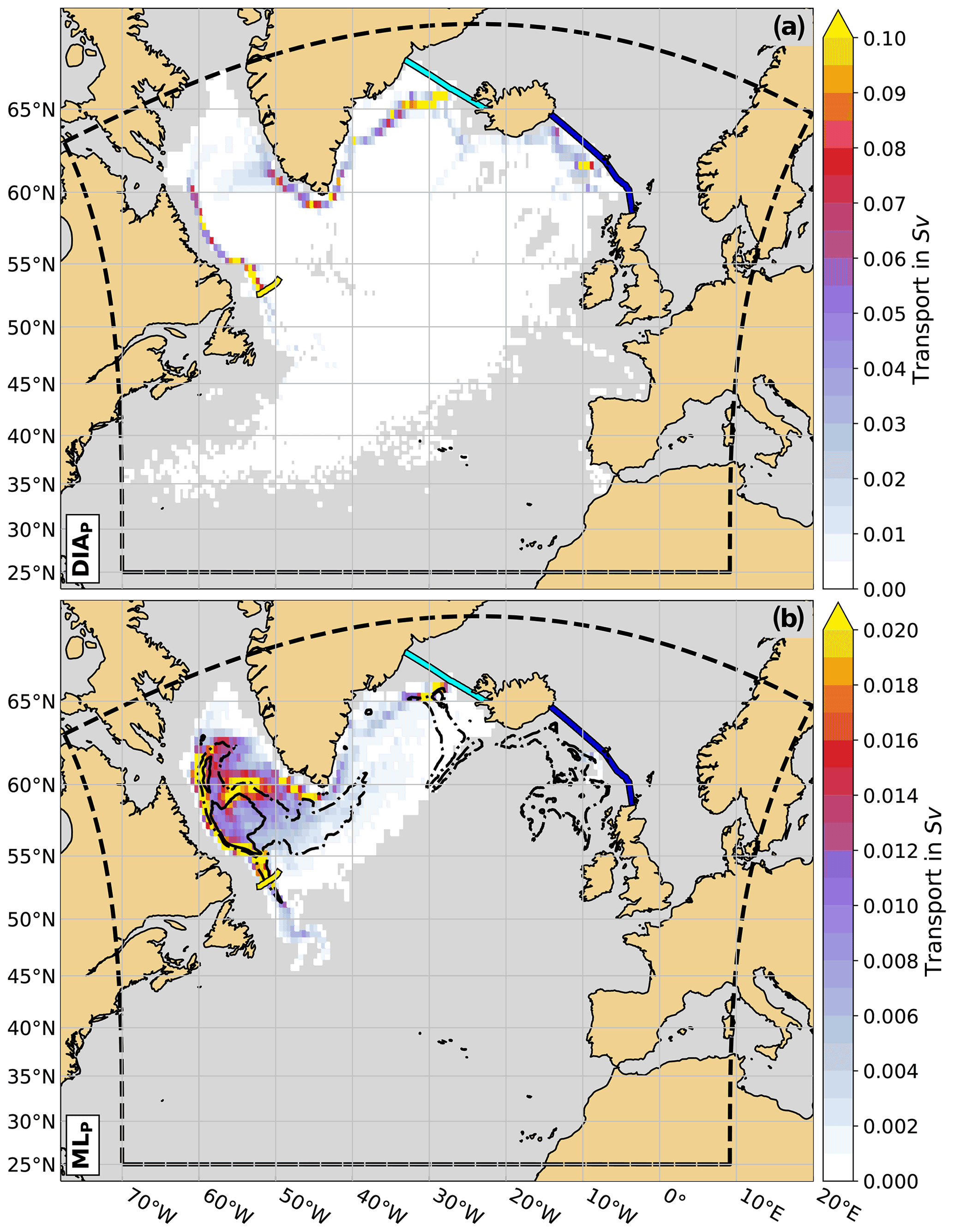
Figure 4Locations of origin, calculated as mean transport (in Sv, shading, bins) for (a) DIAP and (b) MLP (see Sect. 2.1.3 for details of the definitions). (b) The solid black contour marks the 2000–2019 mean December–January–February–March (DJFM) mixed-layer depth of 500 m. The dashed–dotted black contour marks the 2000–2019 mean of the annual maximum mixed-layer depth of 500 m. The period 2000–2019 is chosen to capture the period where the vast majority of MLP is circulating. The yellow line marks the 53∘ N section, and the light and dark blue lines mark the Denmark Strait and Iceland–Scotland Ridge sections, respectively. The dashed black line indicates the boundary of the experiment domain.
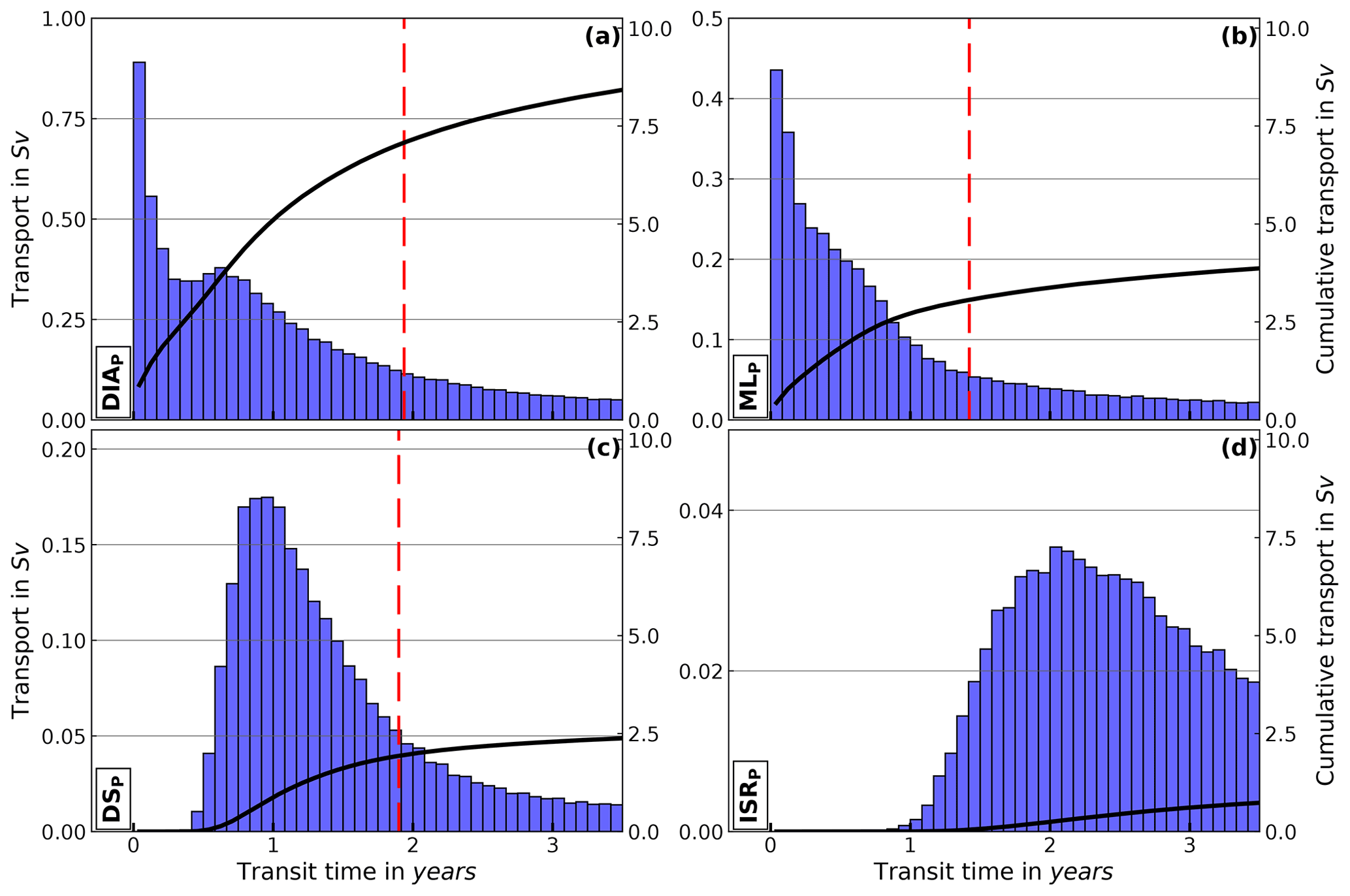
Figure 5Transit time distributions, calculated as mean volume transport in Sv (bars, left-hand y axis) and cumulative mean volume transport in Sv (black lines, right-hand y axis) as a function of transit time (1-month bins) for (a) DIAP, (b) MLP, (c) DSP, and (d) ISRP (see Sect. 2.1.3 for details of the definitions). The dashed red lines mark the time after which half the transport associated with the respective category has reached 53∘ N. Note the different y axis scales for the bar plots.
3.1.1 Diapycnal mass flux
About half the NADW transport at 53∘ N, 14.3 Sv (48 %) is associated with diapycnal mass flux (Table 1). The majority of DIAP enters the NADW density range within the boundary current in the Labrador Sea (5.5 Sv, Table 2) and Irminger Sea (4.6 Sv, Table 2) at depths between 600 and 1000 m (not shown). Only a very small portion is added in the basin interiors (Fig. 4a, Table 2) at depths below 1300 m (not shown). The Iceland basin, adding 2.4 Sv, and the southern SPNA, adding 1.1 Sv, consequently play only a small role for the total NADW with DIAP origin. After their densification, particles of this category spread (Fig. 3a), in addition to the boundary currents, throughout the basin interior of the western SPNA, with further pathways from the Iceland basin following the 1000 m isobath (Figs. 3a and 1) along the Reykjanes Ridge and through the CGFZ. Most particles pass through the central Labrador Sea before exiting it via the DWBC at 53∘ N (Fig. 3a). Most of the DIAP is formed at densities kg m−3, where the Labrador Sea exceeds the Irminger Sea by 1.4 Sv. Similar amounts of lNADW (∼0.5 Sv) are added in both basins, with the Iceland basin and the southern SPNA again only playing a minor role, with 2.2 and 0.8 Sv, respectively (Table 2). The respective maxima of the mean transport are found just south of the DS until 65∘ N, east and west of Cape Farewell, and between Hamilton Bank and 53∘ N. Minor contributing regions are found along the continental slopes south of the ISR, at the Reykjanes Ridge, and within the Labrador Sea (Fig. 4a), most probably following the eddy track of Irminger Rings shed at Cape Desolation (Prater, 2002; Hátún et al., 2007; Rieck et al., 2018). Contrary to the boundary current, the interior does not show as elevated values and a spread over a larger area (Fig. 3a). These patterns of the total NADW are similarly found for the density ranges kg m−3 and σ0≥27.86 kg m−3 (not shown). As the particle sources are located within or nearby boundary currents, which exhibit strong velocities, the particles can have rather short transit times. The transit time distribution peaks between 0 and 1 years, with more than a third of the volume transport associated with DIAP reaching 53∘ N within this time span (Fig. 5a). After approximately 1.94 years, 50 % of the transport associated with DIAP has passed 53∘ N (Fig. 5a).
3.1.2 Mixed layer
The second-largest supplier of NADW, with 7.2 Sv (24 %) of the 30.1 Sv of NADW passing 53∘ N, was found to originate from the mixed layer (MLP, Table 1). The particles leave the mixed layer between November and June, with a peak export between February and April (not shown) dominantly within the central Labrador Sea or the boundary current along the Labrador shelf break (Fig. 4b). Elevated values can also be found south of the DS and west of the Faroe Islands, which could possibly be related to the shallow pathways of the particles at these locations. There are minor but noticeable contributions from the Irminger Sea and southwest of Cape Farewell. These particles tend to leave the mixed layer at shallower depths and lower densities compared to particles from the Labrador Sea (Fig. S1 in the Supplement). The Labrador Sea, however, dominates as source region of this particle category with 5.9 Sv (82 % of the total MLP transport) compared to 1.0 Sv (14 % of the total MLP transport) from the Irminger Sea (Table 2). Within the Labrador Sea, the contribution from the boundary regions dominates with 3.3 Sv over the interior contribution with 2.6 Sv (Table 2). Half of the volume transport associated with MLP reaches 53∘ N within 1.42 years (Fig. 5b), which we expected due to the close proximity of the source regions to 53∘ N.
3.1.3 GSR
With 5.7 Sv (19 %) of the NADW transport at 53∘ N, the water passing the DS (DSP, 3.8 Sv or 13 %) and the ISR (ISRP, 1.9 Sv or 6 %) is the third-largest source of supply for NADW passing 53∘ N (Table 1). These volume transports are comparable to previous model analyses (DS 3.1±0.4 Sv and ISR 1.3±0.2 Sv; Biastoch et al., 2021). These values compare well with the transport estimates from observations, ranging from 3.1 Sv (Jochumsen et al., 2017) to 3.5 Sv (Harden et al., 2016) at DS and are slightly lower than the observed 2.2 Sv (Hansen et al., 2016; Rossby et al., 2018) to 2.7 Sv (Berx et al., 2013) at the ISR.
Particles that pass through the DS within the NADW density range majorly populate the two ∼600 m deep troughs of the strait, with domination of the deeper one just west of Iceland (Fig. 3c). Both pathways then merge south of the DS and follow the East Greenland and West Greenland shelf breaks until reaching the Labrador Sea. DSP has a density between 27.70 and 27.88 kg m−3 (Fig. 2e, v). The longer the particles take to reach 53∘ N, the more particles recirculate through the basin interiors of the Irminger and the Labrador seas (not shown). The transit time distribution peaks between 1 and 2 years of advection (Fig. 5c), with 0 % of the associated transport arriving at 53∘ N within 1.90 years.
NADW particles crossing the ISR are strongly concentrated within the boundary currents after entering the SPNA majorly through the Faroe Bank channel and a trough in the Iceland–Faroe Ridge just east of Iceland (Hvalbakshalli slope, Hjartarson et al., 2017, Fig. 3d). ISRP surround the Reykjanes Ridge between the 1000 and 2000 m isobaths (Figs. 3c and 1) and do not majorly pass through the CGFZ. The longer the particles take to reach 53∘ N, the more particles tend to be advected through the basin interior of the SPNA (not shown). Due to the longer pathways of these particles, transit times tend to be longer. The transit time distribution peaks between 2 and 3 years (Fig. 5d), with 50 % of the associated transport arriving at 53∘ N within 4.78 years. The decay with increasing transit times relative to the peak value is slowest for this category, as a relatively high amount of particles tend to be advected through the basin interior compared to the boundary currents.
Assuming that the shortest transit times are associated with the shortest distances traveled by the particles within a specific particle category, the average velocity a particle must have to reach at least 53∘ N can be calculated. This velocity is estimated to be ∼19 cm s−1 for ISRP and ∼25 cm s−1 for DSP. Similar values are found for particles from the mixed layer and associated with diapycnal mass flux originating from areas close to the GSR. These values seem reasonable given the fact that mean velocities can easily exceed 20 cm s−1 and reach more than 50 cm s−1 at various depth levels in VIKING20X (e.g., Fig. 7 in Biastoch et al., 2021).
3.1.4 Residuum
The volume that is not attributable to any of the above-defined sources of NADW after 40 years of advection amounts to 2.9 Sv (10 %, Table 1). This residuum (RESP) can be separated into particles circulating within the experiment domain for 40 years and particles entering the domain across the southern boundary (25∘ N) or through Davis Strait. Particles circulating for 40 years within the domain contribute 2.1 Sv (72 % of the total RESP transport). Particles entering from the south contribute 0.8 Sv (28 % of the total RESP transport), and particles passing through Davis Strait contribute <0.1 Sv (<2 % of the total RESP transport) (not shown). The majority of RESP recirculate in the basin interior of the SPNA (Fig. S2). The pathways of the denser particles are mostly situated west of the Mid–Atlantic Ridge, while particles with lower densities are advected throughout the whole SPNA. This pattern emerges once the analysis is done in σ2 (not shown). Most particles that cross the Mid-Atlantic Ridge pass through the CGFZ.
3.2 Water mass transformations
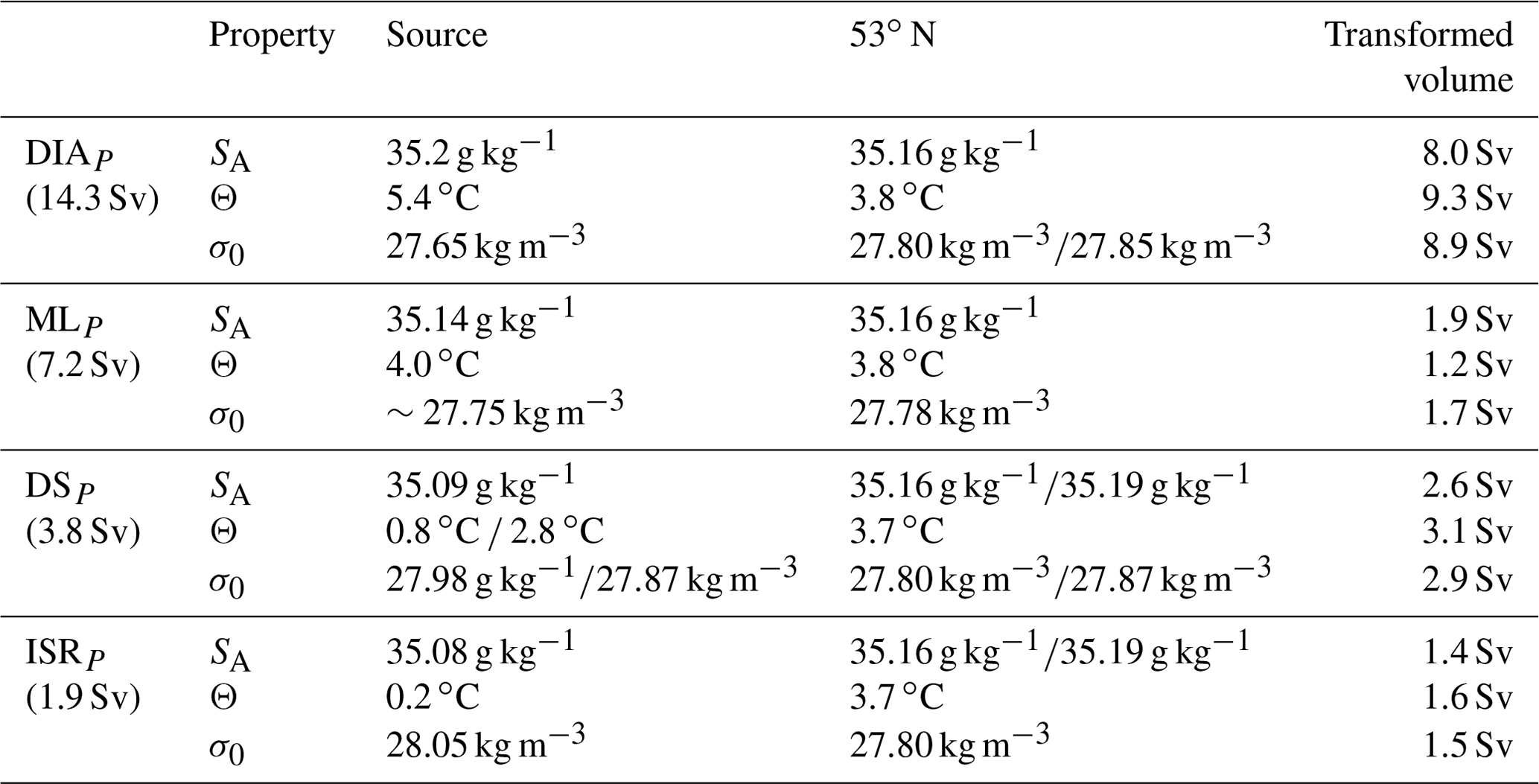
We evaluate the changes that the water parcels undergo during their spreading routes from their point of origin to the 53∘ N target section. The evaluation is done for each particle class (except RESP), ordered by the relative contribution of the respective particle class to the transport at 53∘ N. All particle categories apart from RESP show similar water mass property signatures at 53∘ N. Hence, depending on the properties of absolute salinity (SA), conservative temperature (Θ), and density (σ0) at the point of origin, the water parcels undergo dissimilar changes along their pathways. Particles of DIAP and MLP origin densify through cooling, accompanied by freshening during spreading (Fig. S3), whereas DSP and ISRP lighten through warming, accompanied by salinification from source to target (Fig. S5). In terms of volume, the water mass transformations are more pronounced for DIAP and DSP than for MLP and ISRP (Table 3).
3.2.1 DIAP
The water parcels associated with diapycnal mass flux undergo a significant cooling of ∘C and freshening of g kg−1 along their pathways towards 53∘ N. The freshening value arises from the salinity signature of DIAP at origin and target (Table 3 and Fig. S3).
Freshening occurs mostly along the western flank of the Reykjanes Ridge, along the continental slope around Greenland and off Labrador, and in the interior Labrador Sea (Fig. S4a). East of Cape Farewell, the freshening occurs at depths around 1300 to 1500 m. South of Cape Farewell and Cape Desolation, values reach up to ∼2000 m, while within the Labrador Sea the freshening occurs mostly shallower than 1000 m. South of 53∘ N the transformation can occur at depths deeper than 2000 m; however, these transformations are less important in terms of volume (Fig. S4a, c). Locations and depths of the cooling are similar to the freshening (Fig. S4b, d); however, in terms of volume the cooling is less pronounced along the eastern flank of the Reykjanes Ridge compared to the freshening (Fig. S4a–b).
The cooling dominates over the freshening, leading to a density increase (from σ0=27.65 kg m−3 to σ0=28.05 kg m−3), and narrows the property ranges of all three variables at 53∘ N compared to the source regions. Due to the nature of the diapycnal mass flux the intensive change of particle properties along the spreading pathways between source and target region is not surprising. As described in Sect. 3.1, most DIAP particles originate from the shelf breaks around Greenland and the Labrador Sea and get advected along the boundary current. Here, the elevated property exchange with the ambient shelf water leads to freshening. Additionally, cooling can occur here within the NADW property range due to air–sea exchange.
3.2.2 MLP
At their source regions, particles from the mixed layer are cooler and fresher than DIAP at their respective origin (Table 3). In this experiment particles from the mixed layer majorly originate from the Labrador Sea with a slight domination of the boundary regime (3.3 Sv) over the basin interior (2.6 Sv). A small volume also originates from the southeast of the section and reaches 53∘ N after recirculation at Orphan Knoll (Fig. 4b). Only a relatively small amount of particles originate from the regions where the deepest mixed layers occur (solid black line in Fig. 4b). Due to the definition of the origin of MLP, which is associated with the point where a particle exits the mixed layer within the NADW density range, this is not surprising. The property transition majorly occurs in the marked mixed layer (Fig. 4b), and the water parcels are then advected to the associated point of origin, which is outside of the marked area. Hence, the origin locations only partially coincide with regions where deep mixed layers potentially occur (dashed–dotted black line in Fig. 4b). MLP shows a smaller value range compared to DIAP for all three parameters (Fig. S3). Even though no distinct peak is discernible in the MLP σ0 signature at its origin (Θ=4.0 ∘C, SA=35.14 g kg−1), a slight cooling and salinity increase is apparent, leading to a slight densification (Θ=3.8 ∘C, SA=35.16 g kg−1 and σ0=27.78 kg m−3 (Table 3 and Fig. S3). These properties at the origin and at 53∘ N compare well with literature values for LSW (Liu and Tanhua, 2021). MLP undergoes the least volumetric transformation of the presented particle categories. This is not surprising, as MLP is densified through convection and then, once cut off from the atmosphere, advected majorly adiabatically along isopycnals.
Table 3Mean water mass property modifications of the four particle categories DIAP, MLP, DSP, and ISRP (see Sect. 2.1.3 for details of the definitions). Listed are potential density (referenced to 0 dbar, σ0), absolute salinity (SA), conservative temperature (Θ), and the transformed volume (in Sv) from the source to 53∘ N (target section). When values are presented with “/”, two major classes of properties are persistent for this particle category.
3.2.3 GSR
In contrast to the particles of the DIAP and MLP categories, the DSP and ISRP spread predominantly along the boundary currents. As mentioned before, DSP features a mixture of different water types with similar salinity (SA=35.09 g kg−1) and varying temperature signatures (close to Greenland shelf: Θ=0.8 ∘C; close to Iceland: Θ=2.8 ∘C) within the NADW, but both undergo similar transitions south of the DS (Table 3). DSP and ISRP both feature a decrease in density due to similar property transitions along their spreading pathways, as they undergo a substantial salinity increase and warming (Table 3 and Fig. S5). For the decrease in density, the temperature increase dominates over the increase in salinity. The salinity increase (to the point where 50 % of the total increase is reached) occurs for both particle categories just after crossing the GSR, i.e., close to the East Greenland shelf break just south of the DS (DSP) and along the ISR slope between Iceland and the Faroe Islands (ISRP), within the 1000 and 2000 m isobaths (Figs. S6 and 1) and is followed by a continuous decrease in salinity until 53∘ N (Fig. S7). The major salinity increase is reached at depths that are mostly shallower than 600 m for both categories and implies mixing with the ambient upper AMOC water (Fig. S6). Due to the shallowness of the overflows over the GSR, the mixing of the ISRP and DSP NADW water parcels with warmer and more saline upper AMOC waters just south of the overflows is not surprising. After this strong entrainment at rather shallow depths, the NADW spreads southward along isopycnals that increase their depth towards the south (Fig. S8c, d). Due to this relative sinking and the physical properties of the boundary current, some more diapycnal mixing (between 1000 and 1500 m), less intense than near the GSR, occurs along the eastern and western Greenland slopes. Further enhanced mixing is found south and west of Cape Farewell around the Eirik Ridge at depths between 1500 and 2000 m, which results in further lightening of the DSP and ISRP within the NADW density range.
In order to assess the mean relative contributions of the different sources of NADW passing the southern exit of the Labrador Sea at 53∘ N, a Lagrangian particle experiment was conducted in the high-resolution ocean model VIKING20X-JRA-OMIP. Each particle represents a defined volume and retains it along its trajectory, similar to stream tubes in a steady flow (van Sebille et al., 2017). Since the volume of each particle is preserved, but its properties are allowed to change along its trajectory, this resulted in the evaluation of the various sources, pathways, transit timescales, and property transitions that NADW water parcels are subject to during their spreading from their origin in the SPNA to 53∘ N.
4.1 Origins of NADW in observations vs. VIKING20X-JRA-OMIP
Concerning the volume transports of the respective particle classes, our results are not directly comparable to existing literature. Usually, the transports at 53∘ N are classified after their water mass properties into LSW, NEADW, and DSOW, which are of course related to their origins and have defined properties in temperature, salinity, density, and/or potential vorticity (Zantopp et al., 2017; Liu and Tanhua, 2021). The observations of Zantopp et al. (2017) find a relative contribution of 50:50 of LSW (14.9±3.9 Sv) and lNADW (15.3±3.8 Sv) to the 30 Sv NADW transport at 53∘ N. In contrast to this, using the previously defined water mass definitions in the model (Handmann et al., 2018), we find only a very small amount of the modeled Eulerian NADW water transport of 30.1 Sv at 53∘ N associated with lNADW (3.4 Sv, Table 1). In order to evaluate the respective origin of the total NADW transport at 53∘ N in the model without being biased towards any predefined density interval, we did not use rigid density classes in the following analyses but classified the transport volumes after their specific formation origin. Our experiment reveals that the specific particle categories are not primarily linked to an overall density definition at 53∘ N but rather to a similar formation region in combination with a specific transformation history. Just like the classical understanding of water masses, the densities are ordered with the densest components at the origin in the ISR (σ0=28.05 kg m−3) and DS (σ0=27.98 kg m−3 and σ0=27.87 kg m−3) and the lightest component from the mixed layer (σ0=27.75 kg m−3) (Table 3). For the overflow component, a transport increase from the sills (6 Sv, Jochumsen et al., 2012; Hansen et al., 2010), to the boundary current east of Greenland (9 Sv, Bacon et al., 2010), and to 53∘ N (15 Sv, Zantopp et al., 2017) is observed. In the observations, the lNADW component is hence associated with the formation region in the Nordic Seas plus an added volume through entrainment of ambient water south of the overflow sills at the DS and ISR and through diapycnal mass flux into the respective density class in the SPNA through, e.g., mesoscale eddies. Hence, these additional ∼10 Sv are most probably represented in our analyses by the DIAP water class, even though they do not forcibly belong to the densest component in the model. Biastoch et al. (2021) show comparable Eulerian transports at the GSR between VIKING20X-JRA-OMIP and observations. This coincides with the total NADW sourced at DS (3.8 Sv) found in this experiment (Table 1). As mentioned by Zou et al. (2020b) and Bower and Furey (2017), the water originating from the ISR can spread following very diffusive pathways. As we are only sampling water parcels passing 53∘ N, the 1.9 Sv we found to be originating from the ISR seem to be reasonable (Table 1). Consequently, in the model the dense overflow component from the GSR loses volume towards lighter densities that lie within the predefined LSW density range. This is most probably caused by larger than observed entrainment of light water along the spreading pathway just south of the sill (Beismann and Barnier, 2004; Legg et al., 2009) and underlines a contrast with observations where the lNADW volume grows along the spreading route. On the other hand, in our experiment, the densest water below σ0=27.86 kg m−3 cannot be assigned to a specific source after 40 years of advection (Table 1). Most probably, this dense water is introduced at the initialization of the model and not refreshed or majorly changed and is instead reduced towards lighter densities during the model run. Pathways of RESP are concentrated west of the Mid-Atlantic Ridge (Fig. S2). This is related to the fact that the residuum mostly contains particles with very high densities that recirculate within the western SPNA (Fig. 2b, ii) and are unable to cross the Mid-Atlantic Ridge. To conclude, we find that the density interval with the major transports in NADW at 53∘ N around σ0=27.80 kg m−3 is not only associated with one source. Instead, multiple sources contribute with different relative importance to similar density regimes, though the DIAP and MLP dominate (Fig. 2).
With 48 % of the total NADW and LSW transport, DIAP represents the majority of NADW (LSW) at 53∘ N in this experiment (Table 1). This result aligns with the results of Lumpkin et al. (2008) and Marsh et al. (2005), who found that most of the LSW, leaving the SPNA southward, originates from subsurface diapycnal mixing, without contact to the atmosphere, rather than directly from the mixed layer as a result of air–sea fluxes.
4.2 Origin in the basin interior vs. the boundary current
The DIAP contributing to the NADW transport at 53∘ N is majorly confined to the continental shelf break (Fig. 4a, Table 2). Only small diapycnal mass flux is visible in the central Labrador Sea, possibly due to mixing induced through eddies shed at Cape Desolation and even smaller, nonsignificant numbers are found in the basin interior of the Irminger Sea or the Iceland basin (Fig. 4a, Table 2) (Prater, 2002; Hátún et al., 2007; Rieck et al., 2018). This pattern of densification along the buoyant boundary currents is shown in multiple idealized and realistic model studies (Spall, 2004; Xu et al., 2018; Katsman et al., 2018; Brüggemann and Katsman, 2019; Georgiou et al., 2019; Sidorenko et al., 2020), as well as in observations (Waterhouse et al., 2014). Katsman et al. (2018) show that sinking of water masses occur where friction plays an important role, i.e., close to the continental boundary. However, they only consider downwelling in depth space, and thus the net sinking is not necessarily associated with a change in density. Based on an idealized model, Brüggemann and Katsman (2019) showed that densification can also be related to transport of water masses from lower to higher densities. In this case water masses are advected laterally via mesoscale eddies into the boundary current across an isopycnal, leading to a change in density. The true causes of this pattern, however, need to be explored in more detail in order to elaborate a profound hypothesis based on the model's abilities. Here, the densification is understood as a result of diapycnal volume fluxes and mixing induced by strong density gradients below the mixed layer in the vicinity of steep topographic slopes and a respective enhanced eddy activity (Spall, 2001; Radko and Marshall, 2004; MacKinnon et al., 2013; Zhang et al., 2019). Consequently, the relative contribution of the basin interiors is negligible, as shown above (Table 2).
Additionally, the diapycnal volume fluxes could be further linked to air–sea heat fluxes upstream of the respective NADW origin region through outcropping of the respective isopycnal (Walin, 1982; Grist et al., 2009; Marsh, 2000; Desbruyères et al., 2019; Petit et al., 2020, 2021). The arising density compensated for shifts in temperature and salinity in the Subpolar Mode Water (SPMW) just above the NADW could then facilitate densification along the net sinking pathways of SPMW, though this analysis is beyond the scope of this paper.
4.3 Hydrographic transformations along spreading pathways
Another aspect of diapycnal mixing is featured in the property change in DSP and ISRP, the warming and salinification from the GSR to 53∘ N (Table 3, Fig. S5). These water parcels spread below the main thermocline and gain buoyancy during their southward propagation as expected (MacKinnon et al., 2013). We showed that the major part of the density decrease, at least 50 % of the salinification and warming, occurs south of the GSR sills (Fig. S6). Here, the mixing driving this density transformation is elevated due to enhanced turbulence through the high velocities (exceeding 20 cm s−1 and reaching up to 50 cm s−1) at the sills and the sloping topography (Fig. 1, Rudels et al., 2002; Koszalka et al., 2013; Garabato et al., 2019). This is in agreement with the results of Fogelqvist et al. (2003) and Devana et al. (2021), who find a massive impact of upper-ocean properties on the NADW passing the GSR channels due to high spill velocities enhancing shear instabilities towards the overlying upper AMOC waters. South of the DS, in addition to the upper AMOC waters, fresh and cold East Greenland Current water is another possible ambient water mass to be entrained (Dickson and Brown, 1994). Hence, we conclude in concurrence with Jochumsen et al. (2015) and Devana et al. (2021) that changes in the mixing ratio and the respective water properties of entrained waters can majorly influence the downstream NADW properties originating from the GSR. During the spreading along the boundaries, a net sinking in the depth space of the NADW from the GSR is found (Fig. S8c–d), which is in agreement with Katsman et al. (2018).
For DIAP we found a cooling and freshening between the source and target section (Table 3, Fig. S3). Mixing with colder and fresher water from the basin interior could play a role here (Spall and Pickart, 2003). MLP only shows small property alterations along its spreading pathways that are probably related to the spatial closeness to the 53∘ N target section.
4.4 Contribution from the mixed layer
Consistent with previous studies, both those based on observations and models (Pickart et al., 1997, 2002; Marshall and Schott, 1999; Cuny et al., 2005; Brandt et al., 2007; MacGilchrist et al., 2020; Georgiou et al., 2020), the mixed-layer (MLP) origins contributing majorly to the 53∘ N transport are located within the central Labrador Sea and the Western Boundary Current region in the Labrador Sea (Fig. 4b and Table 2). The contribution from the boundary regions exceeds the direct contribution from the interior (Table 2). In agreement with Koelling et al. (2022), the export of MLP at 53∘ N is between February and April, and the transit times between formation and export are of only a few months (Fig. 5b).
The experiment also shows a small but noticeable contribution from the Irminger Sea and from southeast of Cape Farewell (Table 2 and 1, Fig. 4b). Contributions from these regions are to be expected, since the Irminger Sea and the southern tip of Greenland have been established as additional sites of deep convection (Pickart et al., 2003; Våge et al., 2008; de Jong et al., 2012, 2018; Rühs et al., 2021), although the relative importance of each of them is still under debate. However, the Irminger Sea only plays a minor role in the presented experiment, providing only 1.0 Sv (14 %) of the total volume transport associated with the mixed layer, compared to 5.9 Sv (82 %) from the Labrador Sea (Table 2). The convection area, along with the produced density and volume produced through convection in the Irminger Sea, is comparable to the Labrador Sea in the period 2015–2018 (Rühs et al., 2021). Here, we analyze the period 2010–2019, which does not include the possible strong inter-annual variations in relative contribution of the two basins to the overall mixed-layer contribution to the NADW at 53∘ N. Hence, it is possible that the Irminger Sea contribution is underestimated in the second half of our experiment. Furthermore, in accordance with Le Bras et al. (2020) and Rühs et al. (2021), the shallower components of convective water masses from the Irminger Sea tend to be lighter compared to water masses formed within the Labrador Sea (Fig. S1). Thus, it is possible that particles leaving the mixed layer in the Irminger Sea undergo further transformation along their pathways towards 53∘ N. If these particles experience a reduction in density to values lower than σDW, they would add volume to the SPMW but not to the NADW and are not covered in our experiment. On the other hand, if the density is increased to values higher than σDW again at a later point, these particles would be attributed to a different region or a different source entirely. In agreement with Petit et al. (2020), most of the overturning occurs in the eastern SPNA in the analyzed model. However, contrary to their analysis we focus on the overall AMOC density at OSNAP (27.62 kg m−3) and not at OSNAP East (27.54 kg m−3). Water lighter than 27.62 kg m−3 could be transported from the Irminger Sea to the Labrador Sea and then transformed to σ≥27.62 kg m−3. This difference in the density boundary could be an additional reason for the differences in transformation volumes between our results and their work.
4.5 Pathways of NADW
Due to our experimental setup and as expected from the literature (Kieke and Yashayaev, 2015; Palter et al., 2016; Fischer et al., 2018), NADW is majorly advected within the boundary currents close to the continental slope or the shelf break (Fig. 3). Already west of the Eirik Ridge we noticed an enhanced divergence of the particle pathways, which coincides with trajectories from RAFOS (SOund Fixing And Ranging floats) floats of the OSNAP float program (Zou et al., 2021). Near Cape Desolation the pathways further diverge into the Labrador Sea, becoming less confined (Fig. 3) due to bifurcation and the shedding of Irminger Rings (Cuny et al., 2002; Prater, 2002; Hátún et al., 2007; Higginson et al., 2011; Palter et al., 2016; Rieck et al., 2018). Thus, water parcels are transported along more diverse pathways from Greenland across the Labrador Sea before joining into the more confined DWBC off Labrador.
South of 53∘ N, all particle categories feature a cyclonic recirculation cell around Orphan Knoll (Fig. 3), which is in agreement with previous studies (Lavender et al., 2000; Xu et al., 2010). Hence, a slight NADW volume formation is also possible south of 53∘ N, possibly due to horizontal mixing or ocean–atmosphere interaction. These waters can then recirculate to 53∘ N and the Labrador Sea.
Overall, at 53∘ N the total Labrador Sea contribution (12.0 Sv) to the formation of NADW dominates over the Irminger Sea contribution (5.7 Sv) for the evaluated experiment period (Table 2). This seems to be in contrast with recent observation-based studies. Lozier et al. (2019) state that OSNAP East, rather than OSNAP West, dominates the AMOC in the SPNA. The study by Bower et al. (2009) shows that interior pathways are likely to be at least equally important for the export of NADW from the SPNA. The experiment presented here only takes into account the volume transport at 53∘ N, i.e., the NADW export within the DWBC. Thus, here we do not represent the relative contribution of each basin to the total SPNA NADW southward export, which would reflect the AMOC. Additionally, we analyze the trajectories in bulk, which can lead to the impression of the Labrador Sea dominating in NADW formation. To investigate the changing relative points of origin over time, the analysis that we have done here for the mean could be done for each seeding particle set, but this is beyond the scope of this paper.
In this study we show that multiple sources of NADW passing 53∘ N contribute to similar density regimes. The classical view of density classes being directly linked to a common formation region only partly holds within our experiment. We instead find that different origins in combination with transformation processes such as diapycnal mixing along the pathways lead to water mass properties that can be very similar at the southern exit of the Labrador Sea. We found that water passing the GSR (DSP, ISRP) within the NADW layer lightens within the NADW class through warming, which is accompanied by salinification, just south of the sills by mixing with ambient water. Contrary, NADW water originating from densification through diapycnal mixing (DIAP) or contact with the mixed layer (MLP) instead densifies after entering the NADW density class through cooling, which is accompanied by freshening. Due to our focus on the NADW transport within the DWBC at 53∘ N, in our experiment the volume contribution from the Labrador Sea dominates over the rest of the subpolar North Atlantic. Since we analyzed our experiment in an averaging manner for the period 2010–2019, the inter-annual variability of the different sources is not discussed here. The relative importance of origin regions and transformation processes over time is hence a topic left for further analysis.
The trajectory data analyzed in the current study are available from the corresponding authors upon request.
The supplement related to this article is available online at: https://doi.org/10.5194/os-18-1431-2022-supplement.
PVKH and AB defined and guided the overall research problem and methodology. JF developed and performed the Lagrangian experiment, performed the analyses, and created the figures. JF and PVKH wrote the manuscript. All co-authors discussed the analyses and contributed to the text. All authors agree to be accountable for the content of the work.
The contact author has declared that none of the authors has any competing interests.
Publisher's note: Copernicus Publications remains neutral with regard to jurisdictional claims in published maps and institutional affiliations.
We thank Willi Rath for the support during the experimental setup. We thank Franziska Schwarzkopf for running the VIKING20X-JRA-OMIP model. This work received support by the Initiative and Networking Fund of the Helmholtz Association through the project “Advanced Earth System Modelling Capacity (ESM)”. We also thank the two anonymous reviewers for their constructive reviews that helped to improve our manuscript.
The article processing charges for this open-access publication were covered by the GEOMAR Helmholtz Centre for Ocean Research Kiel.
This paper was edited by Ismael Hernández-Carrasco and reviewed by two anonymous referees.
Bacon, S. et al.: RSS Discovery Cruise 332, 21 August–25 September 2008, Arctic Gateway (WOCE AR7), http://nora.nerc.ac.uk/id/eprint/265429 (last access: 14 September 2022), 2010. a
Beismann, J.-O. and Barnier, B.: Variability of the meridional overturning circulation of the North Atlantic: sensitivity to overflows of dense water masses, Ocean Dynam., 54, 92–106, 2004. a
Berx, B., Hansen, B., Østerhus, S., Larsen, K. M., Sherwin, T., and Jochumsen, K.: Combining in situ measurements and altimetry to estimate volume, heat and salt transport variability through the Faroe–Shetland Channel, Ocean Sci., 9, 639–654, https://doi.org/10.5194/os-9-639-2013, 2013. a
Biastoch, A., Schwarzkopf, F. U., Getzlaff, K., Rühs, S., Martin, T., Scheinert, M., Schulzki, T., Handmann, P., Hummels, R., and Böning, C. W.: Regional imprints of changes in the Atlantic Meridional Overturning Circulation in the eddy-rich ocean model VIKING20X, Ocean Sci., 17, 1177–1211, https://doi.org/10.5194/os-17-1177-2021, 2021. a, b, c, d, e, f, g
Bower, A. S. and Furey, H.: Iceland-Scotland Overflow Water transport variability through the Charlie-Gibbs Fracture Zone and the impact of the North Atlantic Current, J. Geophys. Res.-Oceans, 122, 6989–7012, 2017. a
Bower, A. S., Lozier, M. S., Gary, S. F., and Böning, C. W.: Interior pathways of the North Atlantic meridional overturning circulation, Nature, 459, 243–247, https://doi.org/10.1038/nature07979, 2009. a, b
Brandt, P., Funk, A., Czeschel, L., Eden, C., and Böning, C. W.: Ventilation and Transformation of Labrador Sea Water and Its Rapid Export in the Deep Labrador Current, J. Phys. Ocean., 37, 946–961, https://doi.org/10.1175/JPO3044.1, 2007. a
Brüggemann, N. and Katsman, C. A.: Dynamics of Downwelling in an Eddying Marginal Sea: Contrasting the Eulerian and the Isopycnal Perspective, J. Phys. Ocean., 49, 3017–3035, https://doi.org/10.1175/JPO-D-19-0090.1, 2019. a, b
Chafik, L., Hátún, H., Kjellsson, J., Larsen, K. M. H., Rossby, T., and Berx, B.: Discovery of an unrecognized pathway carrying overflow waters toward the Faroe Bank Channel, Nat. Commun., 11, 1–10, 2020. a
Cuny, J., Rhines, P. B., Niiler, P. P., and Bacon, S.: Labrador Sea Boundary Currents and the Fate of the Irminger Sea Water, J. Phys. Ocean., 32, 627–647, https://doi.org/10.1175/1520-0485(2002)032<0627:LSBCAT>2.0.CO;2, 2002. a, b
Cuny, J., Rhines, P. B., Schott, F., and Lazier, J.: Convection above the Labrador Continental Slope, J. Phys. Ocean., 35, 489–511, https://doi.org/10.1175/JPO2700.1, 2005. a
de Jong, M. F., van Aken, H. M., Våge, K., and Pickart, R. S.: Convective mixing in the central Irminger Sea: 2002–2010, Deep Sea Res. Pt. I, 63, 36–51, 2012. a, b
de Jong, M. F., Oltmanns, M., Karstensen, J., and de Steur, L.: Deep convection in the Irminger Sea observed with a dense mooring array, Oceanography, 31, 50–59, 2018. a, b
Delandmeter, P. and van Sebille, E.: The Parcels v2.0 Lagrangian framework: new field interpolation schemes, Geosci. Model Dev., 12, 3571–3584, https://doi.org/10.5194/gmd-12-3571-2019, 2019. a, b
Desbruyères, D. G., Mercier, H., Maze, G., and Daniault, N.: Surface predictor of overturning circulation and heat content change in the subpolar North Atlantic, Ocean Sci., 15, 809–817, https://doi.org/10.5194/os-15-809-2019, 2019. a, b, c
Devana, M. S., Johns, W. E., Houk, A., and Zou, S.: Rapid Freshening of Iceland Scotland Overflow Water Driven By Entrainment of a Major Upper Ocean Salinity Anomaly, Geophys. Res. Lett., 48, e2021GL094396, https://doi.org/10.1029/2021GL094396, 2021. a, b
Dickson, R. R. and Brown, J.: The production of North Atlantic Deep Water: sources, rates, and pathways, J. Geophys. Res.-Oceans, 99, 12319–12341, 1994. a, b, c
Dietrich, G.: Ozeanographische Probleme der deutschen Forschungsfahrten im Internationalen Geophysikalischen Jahr 1957/58, Deutsche Hydrografische Zeitschrift, 10, 39–61, 1957. a
Fichefet, T. and Maqueda, M. A.: Sensitivity of a global sea ice model to the treatment of ice thermodynamics and dynamics, J. Geophys. Res.-Oceans, 102, 12609–12646, 1997. a
Fischer, J., Karstensen, J., Oltmanns, M., and Schmidtko, S.: Mean circulation and EKE distribution in the Labrador Sea Water level of the subpolar North Atlantic, Ocean Sci., 14, 1167–1183, https://doi.org/10.5194/os-14-1167-2018, 2018. a, b, c
Fogelqvist, E., Blindheim, J., Tanhua, T., Østerhus, S., Buch, E., and Rey, F.: Greenland-Scotland overflow studied by hydro-chemical multivariate analysis, Deep Sea Res. Pt. I, 50, 73–102, 2003. a, b
Fröb, F., Olsen, A., Våge, K., Moore, G. W. K., Yashayaev, I., Jeansson, E., and Rajasakaren, B.: Irminger Sea deep convection injects oxygen and anthropogenic carbon to the ocean interior, Nat. Commun., 7, 1–8, 2016. a
Garabato, A. C. N., Frajka-Williams, E. E., Spingys, C. P., Legg, S., Polzin, K. L., Forryan, A., Abrahamsen, E. P., Buckingham, C. E., Griffies, S. M., and McPhail, S. D.: Rapid mixing and exchange of deep-ocean waters in an abyssal boundary current, P. Natl. Acad. Sci. USA, 116, 13233–13238, 2019. a
Georgiou, S., van der Boog, C. G., Brüggemann, N., Ypma, S. L., Pietrzak, J. D., and Katsman, C. A.: On the interplay between downwelling, deep convection and mesoscale eddies in the Labrador Sea, Ocean Modell., 135, 56–70, 2019. a
Georgiou, S., Ypma, S. L., Brüggemann, N., Sayol, J.-M., van der Boog, C. G., Spence, P., Pietrzak, J. D., and Katsman, C. A.: Direct and indirect pathways of convected water masses and their impacts on the overturning dynamics of the Labrador Sea, J. Geophys. Res.-Oceans, 126, e2020JC016654, https://doi.org/10.1029/2020JC016654, 2020. a, b
Grist, J. P., Marsh, R., and Josey, S. A.: On the relationship between the North Atlantic meridional overturning circulation and the surface-forced overturning streamfunction, J. Climate, 22, 4989–5002, 2009. a
Haine, T., Böning, C., Brandt, P., Fischer, J., Funk, A., Kieke, D., Kvaleberg, E., Rhein, M., and Visbeck, M.: North Atlantic deep water formation in the Labrador Sea, recirculation through the subpolar gyre, and discharge to the subtropics, in: Arctic – Subarctic Ocean Fluxes, Springer, 653–701, 2008. a, b
Handmann, P.: Deep Water Formation and Spreading Dynamics in the subpolar North Atlantic from Observations and high-resolution Ocean Models, PhD thesis, Christian-Albrechts-Universität Kiel, http://oceanrep.geomar.de/48432/ (last access: 14 September 2022), 2019. a, b
Handmann, P., Fischer, J., Visbeck, M., Karstensen, J., Biastoch, A., Böning, C., and Patara, L.: The Deep Western Boundary Current in the Labrador Sea From Observations and a High-Resolution Model, J. Geophys. Res.-Oceans, 123, 2829–2850, 2018. a, b, c, d
Hansen, B., Hátún, H., Kristiansen, R., Olsen, S. M., and Østerhus, S.: Stability and forcing of the Iceland-Faroe inflow of water, heat, and salt to the Arctic, Ocean Sci., 6, 1013–1026, https://doi.org/10.5194/os-6-1013-2010, 2010. a
Hansen, B., Húsgarð Larsen, K. M., Hátún, H., and Østerhus, S.: A stable Faroe Bank Channel overflow 1995–2015, Ocean Sci., 12, 1205–1220, https://doi.org/10.5194/os-12-1205-2016, 2016. a
Hansen, B. and Østerhus, S.: North atlantic–nordic seas exchanges, Prog. Oceanogr., 45, 109–208, 2000. a
Harden, B. E., Pickart, R. S., Valdimarsson, H., Våge, K., de Steur, L., Richards, C., Bahr, F., Torres, D., Børve, E., and Jónsson, S.: Upstream sources of the Denmark Strait Overflow: Observations from a high-resolution mooring array, Deep Sea Res. Pt. I, 112, 94–112, 2016. a
Hátún, H., Eriksen, C. C., and Rhines, P. B.: Buoyant eddies entering the Labrador Sea observed with gliders and altimetry, J. Phys. Ocean., 37, 2838–2854, 2007. a, b, c, d
Higginson, S., Thompson, K., and Huang, J.: The mean surface circulation of the North Atlantic subpolar gyre: A comparison of estimates derived from new gravity and oceanographic measurements, J. Geophys. Res.-Oceans, 116, https://doi.org/10.1029/2010JC006877, 2011. a, b
Hjartarson, A., Erlendsson, Ö., and Blischke, A.: The Greenland–Iceland–Faroe Ridge Complex, Geol. Soc. Spec. Publ., 447, 127–148, https://doi.org/10.1144/SP447.14, 2017. a
Intergovernmental Oceanographic Commission: The International thermodynamic equation of seawater–2010: calculation and use of thermodynamic properties, (includes corrections up to 31st October 2015), 2015. a
Jochumsen, K., Quadfasel, D., Valdimarsson, H., and Jonsson, S.: Variability of the Denmark Strait overflow: Moored time series from 1996–2011, J. Geophys. Res.-Oceans, 117, https://doi.org/10.1029/2012JC008244, 2012. a
Jochumsen, K., Köllner, M., Quadfasel, D., Dye, S., Rudels, B., and Valdimarsson, H.: On the origin and propagation of Denmark Strait overflow water anomalies in the Irminger Basin, J. Geophys. Res.-Oceans Oceans, 120, 1841–1855, 2015. a, b
Jochumsen, K., Moritz, M., Nunes, N., Quadfasel, D., Larsen, K. M. H., Hansen, B., Valdimarsson, H., and Jonsson, S.: Revised transport estimates of the D enmark S trait overflow, J. Geophys. Res.-Oceans, 122, 3434–3450, 2017. a
Johnson, H. L., Cessi, P., Marshall, D. P., Schloesser, F., and Spall, M. A.: Recent contributions of theory to our understanding of the Atlantic meridional overturning circulation, J. Geophys. Res.-Oceans, 124, 5376–5399, 2019. a, b
Jong, M. F. and Steur, L.: Strong winter cooling over the Irminger Sea in winter 2014–2015, exceptional deep convection, and the emergence of anomalously low SST, Geophys. Res. Lett., 43, 7106–7113, 2016. a
Katsman, C., Drijfhout, S., Dijkstra, H., and Spall, M.: Sinking of Dense North Atlantic Waters in a Global Ocean Model: Location and Controls, J. Geophys. Res.-Oceans, 123, 3563–3576, 2018. a, b, c, d, e
Kieke, D. and Yashayaev, I.: Studies of Labrador Sea Water formation and variability in the subpolar North Atlantic in the light of international partnership and collaboration, Prog. Oceanogr., 132, 220–232, 2015. a
Koelling, J., Atamanchuk, D., Karstensen, J., Handmann, P., and Wallace, D. W. R.: Oxygen export to the deep ocean following Labrador Sea Water formation, Biogeosciences, 19, 437–454, https://doi.org/10.5194/bg-19-437-2022, 2022. a
Koszalka, I. M., Haine, T. W. N., and Magaldi, M. G.: Fates and Travel Times of Denmark Strait Overflow Water in the Irminger Basin, J. Phys. Ocean., 43, 2611–2628, https://doi.org/10.1175/JPO-D-13-023.1, 2013. a
Lab Sea Group: The Labrador Sea deep convection experiment, B. Am. Meteorol. Soc., 79, 2033–2058, 1998. a
Lankhorst, M. and Zenk, W.: Lagrangian observations of the middepth and deep velocity fields of the northeastern Atlantic Ocean, J. Phys. Ocean., 36, 43–63, 2006. a
Lavender, K. L., Davis, R. E., and Owens, W. B.: Mid-depth recirculation observed in the interior Labrador and Irminger Seas by direct velocity measurements, Nature, 407, 66–69, 2000. a
Lazier, J.: The renewal of Labrador sea water, Deep Sea Res., 20, 341–353, https://doi.org/10.1016/0011-7471(73)90058-2, 1973. a
Le Bras, I. A.-A., Straneo, F., Holte, J., de Jong, M. F., and Holliday, N. P.: Rapid Export of Waters Formed by Convection Near the Irminger Sea's Western Boundary, Geophys. Res. Lett., 47, e2019GL085989, https://doi.org/10.1029/2019gl085989, 2020. a, b
Legg, S., Ezer, T., Jackson, L., Briegleb, B. P., Danabasoglu, G., Large, W. G., Wu, W., Chang, Y., Ozgokmen, T. M., and Peters, H.: Improving oceanic overflow representation in climate models: The gravity current entrainment climate process team, B. Am. Meteorol. Soc., 90, 657–670, 2009. a
Lilly, J. M., Rhines, P. B., Schott, F., Lavender, K., Lazier, J., Send, U., and D’Asaro, E.: Observations of the Labrador Sea eddy field, Prog. Oceanogr., 59, 75–176, https://doi.org/10.1016/j.pocean.2003.08.013, 2003. a
Liu, M. and Tanhua, T.: Water masses in the Atlantic Ocean: characteristics and distributions, Ocean Sci., 17, 463–486, https://doi.org/10.5194/os-17-463-2021, 2021. a, b, c, d
Lozier, M. S.: Overturning in the North Atlantic, Annu. Rev. Mar. Sci., 4, 291–315, 2012. a
Lozier, M. S., Bacon, S., Bower, A. S., Cunningham, S. A., de Jong, M. F., de Steur, L., deYoung, B., Fischer, J., Gary, S. F., Greenan, B. J. W., Heimbach, P., Holliday, N. P., Houpert, L., Inall, M. E., Johns, W. E., Johnson, H. L., Karstensen, J., Li, F., Lin, X., Mackay, N., Marshall, D. P., Mercier, H., Myers, P. G., Pickart, R. S., Pillar, H. R., Straneo, F., Thierry, V., Weller, R. A., Williams, R. G., Wilson, C., Yang, J., Zhao, J., and Zika, J. D.: Overturning in the Subpolar North Atlantic Program: A New International Ocean Observing System, B. Am. Meteorol. Soc., 98, 737–752, 2017. a
Lozier, M. S., Li, F., Bacon, S., Bahr, F., Bower, A. S., Cunningham, S. A., de Jong, M. F., de Steur, L., deYoung, B., Fischer, J., Gary, S. F., Greenan, B. J. W., Holliday, N. P., Houk, A., Houpert, L., Inall, M. E., Johns, W. E., Johnson, H. L., Johnson, C., Karstensen, J., Koman, G., Le Bras, I. A., Lin, X., Mackay, N., Marshall, D. P., Mercier, H., Oltmanns, M., Pickart, R. S., Ramsey, A. L., Rayner, D., Straneo, F., Thierry, V., Torres, D. J., Williams, R. G., Wilson, C., Yang, J., Yashayaev, I., and Zhao, J.: A sea change in our view of overturning in the subpolar North Atlantic, Science, 363, 516–521, https://doi.org/10.1126/science.aau6592, 2019. a, b, c
Lumpkin, R., Speer, K. G., and Koltermann, K. P.: Transport across 48 N in the Atlantic Ocean, J. Phys. Ocean., 38, 733–752, 2008. a
MacGilchrist, G. A., Johnson, H. L., Marshall, D. P., Lique, C., Thomas, M., Jackson, L. C., and Wood, R. A.: Locations and Mechanisms of Ocean Ventilation in the High-Latitude North Atlantic in an Eddy-Permitting Ocean Model, J. Climate, 33, 10113–10131, https://doi.org/10.1175/JCLI-D-20-0191.1, 2020. a
MacKinnon, J., St Laurent, L., and Naveira Garabato, A. C.: Chapter 7 – Diapycnal Mixing Processes in the Ocean Interior, in: Ocean Circulation and Climate, edited by: Siedler, G., Griffies, S. M., Gould, J., and Church, J. A., Vol. 103 of International Geophysics, Academic Press, 159–183, https://doi.org/10.1016/B978-0-12-391851-2.00007-6, 2013. a, b
Madec, G., Bourdallé-Badie, R., Bouttier, P.-A., Bricaud, C., Bruciaferri, D., Calvert, D., Chanut, J., Clementi, E., Coward, A., Delrosso, D., Ethé, C., Flavoni, S., Graham, T., Harle, J., Iovino, D., Lea, D., Lévy, C., Lovato, T., Martin, N., Masson, S., Mocavero, S., Paul, J., Rousset, C., Storkey, D., Storto, A., and Vancoppenolle, M.: NEMO ocean engine, Zenodo, https://doi.org/10.5281/zenodo.1472492, 2017. a
Marsh, R.: Recent variability of the North Atlantic thermohaline circulation inferred from surface heat and freshwater fluxes, J. Climate, 13, 3239–3260, 2000. a
Marsh, R., De Cuevas, B. A., Coward, A. C., Bryden, H. L., and Álvarez, M.: Thermohaline circulation at three key sections in the North Atlantic over 1985–2002, Geophys. Res. Lett., 32, https://doi.org/10.1029/2004GL022281, 2005. a
Marshall, J. and Schott, F.: Open-ocean convection: Observations, theory, and models, Rev. Geophys., 37, 1–64, https://doi.org/10.1029/98RG02739, 1999. a, b, c
Mertens, C., Rhein, M., Walter, M., Böning, C. W., Behrens, E., Kieke, D., Steinfeldt, R., and Stöber, U.: Circulation and transports in the Newfoundland Basin, western subpolar North Atlantic, J. Geophys. Res.-Oceans, 119, 7772–7793, 2014. a
Molinari, R. L., Fine, R. A., Wilson, W. D., Curry, R. G., Abell, J., and McCartney, M. S.: The arrival of recently formed Labrador sea water in the Deep Western Boundary Current at 26.5∘ N, Geophys. Res. Lett., 25, 2249–2252, https://doi.org/10.1029/98GL01853, 1998. a
Palter, J. B., Caron, C.-A., Law, K. L., Willis, J. K., Trossman, D. S., Yashayaev, I. M., and Gilbert, D.: Variability of the directly observed, middepth subpolar North Atlantic circulation, Geophys. Res. Lett., 43, 2700–2708, https://doi.org/10.1002/2015gl067235, 2016. a, b, c, d
Petit, T., Lozier, M. S., Josey, S. A., and Cunningham, S. A.: Atlantic deep water formation occurs primarily in the Iceland Basin and Irminger Sea by local buoyancy forcing, Geophys. Res. Lett., 47, e2020GL091028, https://doi.org/10.1029/2020GL091028, 2020. a, b, c, d
Petit, T., Lozier, M. S., Josey, S. A., and Cunningham, S. A.: Role of air–sea fluxes and ocean surface density in the production of deep waters in the eastern subpolar gyre of the North Atlantic, Ocean Sci., 17, 1353–1365, https://doi.org/10.5194/os-17-1353-2021, 2021. a
Pickart, R. S.: Water mass components of the North Atlantic deep western boundary current, Deep Sea Res., 39, 1553–1572, 1992. a
Pickart, R. S. and Spall, M. A.: Impact of Labrador Sea Convection on the North Atlantic Meridional Overturning Circulation, J. Phys. Oceanogr., 37, 2207–2227, https://doi.org/10.1175/jpo3178.1, 2007. a
Pickart, R. S., Spall, M. A., and Lazier, J. R.: Mid-depth ventilation in the western boundary current system of the sub-polar gyre, Deep Sea Res. Pt. I, 44, 1025–1054, https://doi.org/10.1016/S0967-0637(96)00122-7, 1997. a, b, c
Pickart, R. S., Torres, D. J., and Clarke, R. A.: Hydrography of the Labrador Sea during Active Convection, J. Phys. Ocean., 32, 428–457, https://doi.org/10.1175/1520-0485(2002)032<0428:HOTLSD>2.0.CO;2, 2002. a
Pickart, R. S., Spall, M. A., Ribergaard, M. H., Moore, G. W. K., and Milliff, R. F.: Deep convection in the Irminger Sea forced by the Greenland tip jet, Nature, 424, 152–156, https://doi.org/10.1038/nature01729, 2003. a
Piron, A., Thierry, V., Mercier, H., and Caniaux, G.: Argo float observations of basin-scale deep convection in the Irminger sea during winter 2011–2012, Deep Sea Res. Pt. I, 109, 76–90, https://doi.org/10.1016/j.dsr.2015.12.012, 2016. a
Prater, M. D.: Eddies in the Labrador Sea as observed by profiling RAFOS floats and remote sensing, J. Phys. Ocean., 32, 411–427, 2002. a, b, c, d
Radko, T. and Marshall, J.: Eddy-Induced Diapycnal Fluxes and Their Role in the Maintenance of the Thermocline, J. Phys. Ocean., 34, 372–383, https://doi.org/10.1175/1520-0485(2004)034<0372:EDFATR>2.0.CO;2, 2004. a
Rhein, M., Kieke, D., Hüttl-Kabus, S., Roessler, A., Mertens, C., Meissner, R., Klein, B., Böning, C. W., and Yashayaev, I.: Deep water formation, the subpolar gyre, and the meridional overturning circulation in the subpolar North Atlantic, Deep Sea Res. Pt II, 58, 1819–1832, 2011. a
Rhein, M., Rintoul, S., Aoki, S., Campos, E., Chambers, D., Feely, R., Gulev, S., Johnson, G., Josey, S., Kostianoy, A., et al.: Observations: ocean, Cambridge University Press, 255–316, https://doi.org/10.1017/CBO9781107415324.010, 2013. a
Rieck, J. K., Böning, C., and Getzlaff, K.: The Nature of Eddy Kinetic Energy in the Labrador Sea: Different Types of Mesoscale Eddies, their Temporal Variability and Impact on Deep Convection, J. Phys. Ocean., 49, 2075–2094, 2018. a, b, c, d, e
Rossby, T., Flagg, C., Chafik, L., Harden, B., and Søiland, H.: A Direct Estimate of Volume, Heat, and Freshwater Exchange Across the Greenland‐Iceland‐Faroe‐Scotland Ridge, J. Geophys. Res.-Oceans, 123, 7139–7153, 2018. a
Rudels, B., Eriksson, P., Fahrbach, E., Budéus, G., and Meincke, J.: The East Greenland Current and its contribution to the Denmark Strait overflow, ICES J. Mar. Sci., 59, 1133–1154, 2002. a
Rühs, S., Oliver, E. C. J., Biastoch, A., Böning, C. W., Dowd, M., Getzlaff, K., Martin, T., and Myers, P. G.: Changing spatial patterns of deep convection in the subpolar North Atlantic, J. Geophys. Res.-Oceans, 126, e2021JC017245, https://doi.org/10.1029/2021JC017245, 2021. a, b, c, d, e, f
Sayol, J.-M., Dijkstra, H., and Katsman, C.: Seasonal and regional variations of sinking in the subpolar North Atlantic from a high-resolution ocean model, Ocean Sci., 15, 1033–1053, https://doi.org/10.5194/os-15-1033-2019, 2019. a
Schmidt, C., Schwarzkopf, F. U., Rühs, S., and Biastoch, A.: Characteristics and robustness of Agulhas leakage estimates: an inter-comparison study of Lagrangian methods, Ocean Sci., 17, 1067–1080, https://doi.org/10.5194/os-17-1067-2021, 2021. a, b
Schott, F. A., Fischer, J., Dengler, M., and Zantopp, R.: Variability of the deep western boundary current east of the Grand Banks, Geophys. Res. Lett., 33, https://doi.org/10.1029/2006GL026563, 2006. a
Sidorenko, D., Danilov, S., Fofonova, V., Cabos, W., Koldunov, N., Scholz, P., Sein, D. V., and Wang, Q.: AMOC, Water Mass Transformations, and Their Responses to Changing Resolution in the Finite-VolumE Sea Ice-Ocean Model, J. Adv. Model. Earth Sy., 12, https://doi.org/10.1029/2020MS002317, 2020. a
Spall, M. A.: Large-Scale Circulations Forced by Localized Mixing over a Sloping Bottom, J. Phys. Ocean., 31, 2369–2384, https://doi.org/10.1175/1520-0485(2001)031<2369:LSCFBL>2.0.CO;2, 2001. a
Spall, M. A.: Boundary Currents and Watermass Transformation in Marginal Seas, J. Phys. Ocean., 34, 1197–1213, https://doi.org/10.1175/1520-0485(2004)034<1197:BCAWTI>2.0.CO;2, 2004. a
Spall, M. A. and Pickart, R. S.: Wind-driven recirculations and exchange in the Labrador and Irminger Seas, J. Phys. Ocean., 33, 1829–1845, 2003. a
Stramma, L., Kieke, D., Rhein, M., Schott, F., Yashayaev, I., and Koltermann, K. P.: Deep water changes at the western boundary of the subpolar North Atlantic during 1996 to 2001, Deep Sea Res. Pt. I, 51, 1033–1056, 2004. a
Straneo, F.: On the connection between dense water formation, overturning, and poleward heat transport in a convective basin, J. Phys. Ocean., 36, 1822–1840, 2006. a, b
Tsujino, H., Urakawa, S., Nakano, H., Small, R. J., Kim, W. M., Yeager, S. G., Danabasoglu, G., Suzuki, T., Bamber, J. L., Bentsen, M., Böning, C. W., Bozec, A., Chassignet, E. P., Curchitser, E., Boeira Dias, F., Durack, P. J., Griffies, S. M., Harada, Y., Ilicak, M., Josey, S. A., Kobayashi, C., Kobayashi, S., Komuro, Y., Large, W. G., Le Sommer, J., Marsland, S. J., Masina, S., Scheinert, M., Tomita, H., Valdivieso, M., and Yamazaki, D.: JRA-55 based surface dataset for driving ocean–sea-ice models (JRA55-do), Ocean Modell., 130, 79–139, https://doi.org/10.1016/j.ocemod.2018.07.002, 2018. a
Våge, K., Pickart, R. S., Moore, G. W. K., and Ribergaard, M. H.: Winter mixed layer development in the central Irminger Sea: The effect of strong, intermittent wind events, J. Phys. Ocean., 38, 541–565, 2008. a
Våge, K., Pickart, R. S., Thierry, V., Reverdin, G., Lee, C. M., Petrie, B., Agnew, T. A., Wong, A., and Ribergaard, M. H.: Surprising return of deep convection to the subpolar North Atlantic Ocean in winter 2007–2008, Nat. Geosci., 2, 67–72, 2009. a
van Sebille, E., Baringer, M. O., Johns, W. E., Meinen, C. S., Beal, L. M., de Jong, M. F., and van Aken, H. M.: Propagation pathways of classical Labrador Sea water from its source region to 26∘ N, J. Geophys. Res, 116, C12027, https://doi.org/10.1029/2011JC007171, 2011. a
van Sebille, E., Griffies, S. M., Abernathey, R., Adams, T. P., Berloff, P., Biastoch, A., Blanke, B., Chassignet, E. P., Cheng, Y., Cotter, C. J., et al.: Lagrangian ocean analysis: fundamentals and practices, Ocean Modell., 121, 49–75, 2017. a, b
Walin, G.: On the relation between sea-surface heat flow and thermal circulation in the ocean, Tellus, 34, 187–195, 1982. a
Waterhouse, A. F., MacKinnon, J. A., Nash, J. D., Alford, M. H., Kunze, E., Simmons, H. L., Polzin, K. L., Laurent, L. C. S., Sun, O. M., Pinkel, R., Talley, L. D., Whalen, C. B., Huussen, T. N., Carter, G. S., Fer, I., Waterman, S., Garabato, A. C. N., Sanford, T. B., and Lee, C. M.: Global Patterns of Diapycnal Mixing from Measurements of the Turbulent Dissipation Rate, J. Phys. Ocean., 44, 1854–1872, https://doi.org/10.1175/JPO-D-13-0104.1, 2014. a
Willebrand, J., Barnier, B., Böning, C., Dieterich, C., Killworth, P. D., Le Provost, C., Jia, Y., Molines, J.-M., and New, A. L.: Circulation characteristics in three eddy-permitting models of the North Atlantic, Prog. Oceanogr., 48, 123–161, 2001. a
Xu, X., Schmitz W., J., Hurlburt H., E., Hogan P., J., and Chassignet E., P.: Transport of Nordic Seas overflow water into and within the Irminger Sea: An eddy-resolving simulation and observations, J. Geophys. Res., 115, https://doi.org/10.1029/2010jc006351, 2010. a, b
Xu, X., Rhines, P. B., and Chassignet, E. P.: On mapping the diapycnal water mass transformation of the upper North Atlantic Ocean, J. Phys. Oceanogr., 48, 2233–2258, 2018. a, b
Yashayaev, I. and Loder, J. W.: Recurrent replenishment of Labrador Sea Water and associated decadal-scale variability, J. Geophys. Res.-Oceans, 121, 8095–8114, https://doi.org/10.1002/2016JC012046, 2016. a
Yashayaev, I., Holliday, N. P., Bersch, M., and van Aken, H. M.: The History of the Labrador Sea Water: Production, Spreading, Transformation and Loss, in: Arctic-Subarctic Ocean Fluxes: Defining the Role of the Northern Seas in Climate, Springer Netherlands, Dordrecht, 569–612, https://doi.org/10.1007/978-1-4020-6774-7_25, 2008. a
Yeager, S., Castruccio, F., Chang, P., Danabasoglu, G., Maroon, E., Small, J., Wang, H., Wu, L., and Zhang, S.: An Outsized Role for the Labrador Sea in the Multidecadal Variability of the Atlantic Overturning Circulation, EarthArXiv [preprint], https://doi.org/10.31223/X5ZP68, 2021. a
Zantopp, R., Fischer, J., Visbeck, M., and Karstensen, J.: From interannual to decadal: 17 years of boundary current transports at the exit of the Labrador Sea, J. Geophys. Res.-Oceans, 122, 1724–1748, https://doi.org/10.1002/2016JC012271, 2017. a, b, c, d, e
Zhang, R., Sutton, R., Danabasoglu, G., Kwon, Y., Marsh, R., Yeager, S. G., Amrhein, D. E., and Little, C. M.: A review of the role of the Atlantic Meridional Overturning Circulation in Atlantic multidecadal variability and associated climate impacts, Rev. Geophys., 57, 316–375, 2019. a
Zou, S. and Lozier, M. S.: Breaking the Linkage Between Labrador Sea Water Production and Its Advective Export to the Subtropical Gyre, J. Phys. Oceanogr., 46, 2169–2182, https://doi.org/10.1175/jpo-d-15-0210.1, 2016. a, b
Zou, S., Bower, A. S., Furey, H., Lozier, S. M., and Xu, X.: Redrawing the Iceland-Scotland Overflow Water pathways in the North Atlantic, Nat. Commun., 11, 1890, https://doi.org/10.1038/s41467-020-15513-4, 2020a. a
Zou, S., Lozier, M. S., Li, F., Abernathey, R., and Jackson, L.: Density-compensated overturning in the Labrador Sea, Nat. Geosci., 13, 121–126, https://doi.org/10.1038/s41561-019-0517-1, 2020b. a
Zou, S., Bower, A. S., Furey, H., Pickart, R. S., Houpert, L., and Holliday, N. P.: Observed Deep Cyclonic Eddies around Southern Greenland, J. Phys. Ocean., 51, 3235–3252, 2021. a
Østerhus, S., Turrell, W. R., Hansen, B., Lundberg, P., and Buch, E.: Observed transport estimates between the North Atlantic and the Arctic Mediterranean in the Iceland–Scotland region, Polar Res., 20, 169–175, 2001. a