the Creative Commons Attribution 4.0 License.
the Creative Commons Attribution 4.0 License.
 | 14 Sep 2022
Global coarse-grained mesoscale eddy statistics based on integrated kinetic energy and enstrophy correlations
Imre M. Jánosi
Holger Kantz
Jason A. C. Gallas
Miklós Vincze
Recently, Jánosi et al. (2019) introduced the concept of a “vortex proxy” based on an observation of strong correlations between integrated kinetic energy and integrated enstrophy over a large enough surface area. When mesoscale vortices are assumed to exhibit a Gaussian shape, the two spatial integrals have particularly simple functional forms, and a ratio of them defines an effective radius of a “proxy vortex”. In the original work, the idea was tested over a restricted area in the Californian Current System. Here we extend the analysis to global scale by means of 25 years of AVISO altimetry data covering the (ice-free) global ocean. The results are compared with a global vortex database containing over 64 million mesoscale eddies. We demonstrate that the proxy vortex representation of surface flow fields also works globally and provides a quick and reliable way to obtain coarse-grained vortex statistics. Estimated mean eddy sizes (effective radii) are extracted in very good agreement with the data from the vortex census. Recorded eddy amplitudes are directly used to infer the kinetic energy transported by the mesoscale vortices. The ratio of total and eddy kinetic energies is somewhat higher than found in previous studies. The characteristic westward drift velocities are evaluated by a time-lagged cross-correlation analysis of the kinetic energy fields. While zonal mean drift speeds are in good agreement with vortex trajectory evaluation in the latitude bands 30–5∘ S and 5–30∘ N, discrepancies are exhibited mostly at higher latitudes on both hemispheres. A plausible reason for somewhat different drift velocities obtained by eddy tracking and cross-correlation analysis is the fact that the drift of mesoscale eddies is only one component of the surface flow fields. Rossby wave activities, coherent currents, and other propagating features on the ocean surface apparently contribute to the zonal transport of kinetic energy.
- Article
(27803 KB) - Full-text XML
- BibTeX
- EndNote


Mesoscale eddies (MEs) at spatial scales from approximately 50 up to 500 km are energetic patterns of ocean surface flow fields. The birth of MEs often occurs along shorelines triggered by shear-driven barotropic instabilities or at the edges of surface currents by density-anomaly-driven baroclinic instabilities (Willett et al., 2006; Chelton et al., 2007; Smith, 2007; Badin et al., 2009; Chelton et al., 2011; Faghmous et al., 2015; Marta and Isachsen, 2018; Brach et al., 2018; Pnyushkov et al., 2018; Cetina-Heredia et al., 2019; van Sebille et al., 2020; Chérubin et al., 2021; Wichmann et al., 2021). The observation of mesoscale vortices on global ocean surfaces is usually based on satellite altimetry, which determines local sea surface heights with respect to the geoid by return time analysis of reflected microwave pulses (Stammer and Cazenave, 2017). Local sea level anomalies (SLAs) are obtained by removing local long-term mean sea surface height (SSH) values. 2D velocity fields are obtained by assuming geostrophic equilibrium at which horizontal (hydrostatic) pressure gradient forces are compensated for by the Coriolis effect. Several Eulerian methods have been developed to identify and locate mesoscale vortices from surface flow fields, most of them based on some form of finding close contours of SLA (Chelton et al., 2011; Mason et al., 2014; Li et al., 2016; Schütte et al., 2016; Pessini et al., 2018; Zhibing et al., 2022). Alternatives use the geometry of the velocity vectors (Nencioli et al., 2010; Ji et al., 2018), contours of the Okubo–Weiss parameter (Chelton et al., 2007; Kurian et al., 2011; Ubelmann and Fu, 2011; Schütte et al., 2016; Pessini et al., 2018), or wavelet analysis (Rubio et al., 2009; Pnyushkov et al., 2018). Detailed comparisons show that all Eulerian methods have pros and cons, and none of them is superior to another (Souza et al., 2011; Escudier et al., 2016). Methods based on identifying Lagrangian coherent structures obey a much better mathematical foundation (Haller, 2015; Beron-Vera et al., 2018; Haller et al., 2018; El Aouni, 2021; Ryzhov and Berloff, 2022). However, they are computationally rather demanding and the (relatively low) spatial resolution of the input fields is a challenging aspect of them (Amores et al., 2018).
Kinetic energy (KE) is a quantitative characteristic of ocean flow fields (Wunsch and Ferrari, 2004; Stammer, 1997; Wunsch, 2009, 2013). KE is usually separated into the mean KE and the eddy KE (EKE) computed from the time-varying velocities; see Fig. 1. Recent data evaluation of satellite observations suggests that eddy-rich regions exhibit a significant increase in mesoscale variability (thus EKE per unit volume), while the equatorial oceans show a decrease in EKE (Martínez-Moreno et al., 2019, 2021).
In this work we extend a previous analysis by Jánosi et al. (2019) to the global scale based on the observation that integrated EKE and integrated enstrophy over a large enough area are strongly correlated in time. A coarse-grained approach can reveal useful information such as mean eddy size or the fraction of vortex energy in total EKE, similarly to a recent study by Rai et al. (2021) wherein oceanic eddy killing by wind was analyzed. In the next section we briefly summarize the essential points of the aforementioned methodology. Then we demonstrate the presence of strong correlations between integrated kinetic energy and enstrophy, and we obtain effective “proxy vortex” radii globally. (In Jánosi et al., 2019, the term “super vortex” was coined to characterize the surface flow field by a single Gaussian vortex; here we rather use proxy vortex to avoid overstatement.) Note that we restrict our analysis to 2D surface flow fields, and vertical vortex structures are not considered. We validate the procedure by comparing the results with data on 64 million mesoscale vortices identified by the most common closed contour method (Faghmous et al., 2015). In addition, we analyze the amplitude relationships between our method and the global vortex census. Finally, we provide a global survey of westward drift constructed by measuring temporal cross-correlations of kinetic energies; discrepancies are discussed.
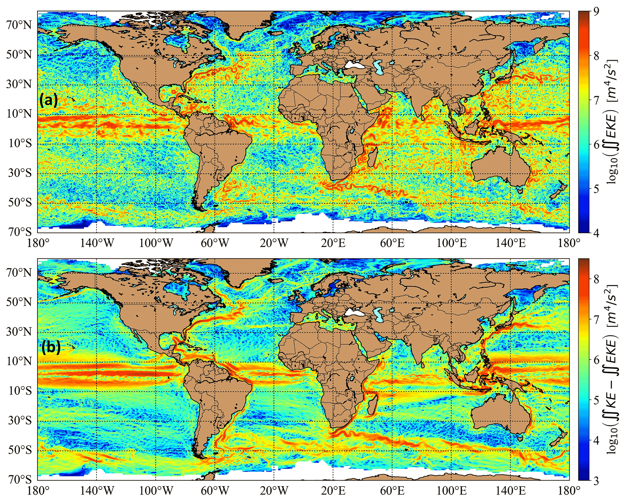
Figure 1Snapshot of the global geostrophic flow field on a randomly chosen day (23 September 2018) from the AVISO data bank (Aviso, 1993–2018; Taburet et al., 2019). Color coding is in a logarithmic scale for better visualization; note the different ranges. (a) Integrated eddy kinetic energy for each grid cell of from geostrophic velocity anomalies (units: m4 s−2). Velocity anomalies [] are obtained from the AVISO data bank; see Sect. 2.1. (b) The difference between the total kinetic energy from geostrophic velocities [ug,vg] and the eddy kinetic energy . Direct [ug,vg] components are determined from sea surface height (SSH) data in the AVISO data bank. Integration is performed by multiplying the squared velocity difference by the curvature-corrected cell size measured in square meters (m2).
2.1 Data sources
Our primary data source is the AVISO data bank (Aviso, 1993–2018; Taburet et al., 2019).
Besides sea level anomalies, geostrophic velocity components and their anomalies are also available. Absolute zonal and meridional velocity components (ugos and vgos in AVISO, denoted here by [ug,vg]) were derived from sea surface height (SSH) data above geoid with the geostrophic balance relations. The absolute velocity components are related to the absolute dynamic topography, which is the sum of sea level anomaly and the mean absolute dynamic topography (MDT). MDT is one of the key quantities to characterize persistent ocean surface currents. Geostrophic velocity anomalies (ugosa and vgosa, []) were computed by removing 20-year mean values (over the period of 1993–2012) for each grid cell (Aviso, 1993–2018; Taburet et al., 2019). In general, geostrophic velocity anomalies are related to mesoscale eddies representing deviations from the mean flow (Frenger et al., 2015; Ji et al., 2018). Figure 1a illustrates the geographic distribution of integrated eddy kinetic energy obtained from geostrophic velocity anomalies [] as , while Fig. 1b is determined from the difference between absolute kinetic energy and eddy kinetic energy as . Figure 1a is supposed to characterize eddy activities, while Fig. 1b is related to the persistent energetic ocean currents. The overlap of red bands in Fig. 1a and b indicates intense vortex shedding along the major currents; however, it cannot be separated from the effects of meandering and relocation of the main currents. The spatial resolution of AVISO fields is (1440 × 720 grid cells), and land areas are masked. The temporal resolution is 1 d in the period 1 January 1993–23 October 2018, with 9397 d without missing dates. Total and eddy kinetic energies (KE and EKE) are obtained trivially from [ug,vg] and [], and enstrophy (the squared vorticity) is determined from the curl of the velocity field (by centered numerical derivatives). Since this operation does not work directly along the shorelines (at least one grid cell should be omitted), we matched the fields properly for an appropriate comparison.
For the validation, we exploited the vortex data bank assembled by Faghmous et al. (2015). They determined mesoscale eddies from the same AVISO data that we utilized, but covering a somewhat shorter temporal period (1 January 1993–2 May 2014, 7791 d). During this period they identified 32 687 988 cyclonic and 31 872 899 anticyclonic eddies globally. Several parameters are stored about each vortex (geographic location, size, major and minor axis lengths from a fit to an ellipsoid, major axis orientation, amplitude, area, etc.); however, we used a limited subset of such data, as explained in Sect. 3 (“Results and discussion” section).
We are aware of the fact that there is a continuously growing set of data repositories, most of them based on AVISO altimetry. We recently learned about the recent development by Pegliasco et al. (2022), which lists several alternatives (Chelton et al., 2007, 2011; Tian et al., 2020; Zhang et al., 2013; Martínez-Moreno et al., 2019). Our choice of Faghmous et al. (2015) was merely determined by the easy access, transparent data format, and large number of eddies in the census. Furthermore, since the vortex detection methods are very similar, we do not expect any large difference between data banks with our coarse-grained methodology.
2.2 Gaussian mesoscale eddies
Several studies of the shape of ocean MEs revealed that they are close to Gaussian humps or troughs (Hopfinger and van Heijst, 1993; Chelton et al., 2011; Raj et al., 2016; Keppler et al., 2018; Martínez-Moreno et al., 2019). A detailed fitting procedure of about 5 million SLA profiles by Wang et al. (2015) revealed that around 50 % of MEs are indeed well approximated by a Gaussian shape:
where η0 is the peak height, r is the radial distance from the vortex center, and R is a radius parameter. Note that R belongs to the 1σ standard deviation of a Gaussian profile, which is not necessarily identified as the radius of an ME by closed contour methods. Besides the Gaussian eddies, another ∼ 40 % are Gaussian over a sloping background or merger of two nearby Gaussian eddies, and the rest have a quadratic core resembling Rankine vortices. Geostrophic equilibrium velocities in polar coordinates have only nonzero tangential components :
where g is the gravitational acceleration, and f=2Ωsin (φ) is the local Coriolis parameter at latitude φ with s−1 for the Earth. The vertical vorticity component ξ(r) is the curl of Eq. (2) in cylindrical coordinates, as usual.
We do not repeat all the details described in Jánosi et al. (2019); we just recall the most important observations. For an isolated Gaussian vortex, the total eddy kinetic energy and enstrophy are finite over an infinite domain of integration (written in 2D polar coordinates):
The total eddy kinetic energy integral IEKE depends only on the peak height η0 of the vortex at a given geographic latitude. The total enstrophy integral IZ is very similar but has an effective radius Reff. That is why the ratio of the two integrals is simply
When the time series of the two integrals are properly correlated, the ratio provides a key to estimate an effective size for a single proxy vortex characterizing the given area of integration. The radius parameter R in Eqs. (1)–(2) and the parameter Reff in Eq. (5) are equivalent in the case of an isolated vortex. However, when we use the spatially integrated kinetic energy and enstrophy ratios over the ocean, the integrals can belong to a couple of eddies. There is no a priori argument regarding why the real radius characterizing the size of an isolated eddy should be closely related to an Reff parameter related to several eddies (apart from the dimension).
We note here that a Gaussian vortex represents a specific case of a general class of solutions of the vorticity equation. The nondimensional form of the tangential velocity field is , where q is the so-called steepness parameter controlling the shape (Carton and Mcwilliams, 1989; Hopfinger and van Heijst, 1993). For any q>0 integer or non-integer case, the spatial integrals of the kinetic energy and enstrophy are finite over an infinite domain of integration usually expressed by the Γ function. Consequently, the ratio of the two integrals is also some rational number. It is an empirical finding (described in the first paragraph in this subsection) that the Gaussian vortex approximation (q=2) works well for mesoscale eddies.
2.3 Analysis of correlations
In order to characterize correlations for the two integrals IEKE and IZ, we determined the Pearson correlation coefficient P by using the standard definition
where angle brackets 〈⋅〉t indicate temporal mean values, and σ is the standard deviation. All calculations were performed in a Python environment (version 3.6) with the standard Numpy (Harris et al., 2020) and SciPy (Virtanen et al., 2020) packages.
Maps were drawn by the Basemap module (https://matplotlib.org/basemap/, last access: 27 April 2022).
Pearson correlation is the most common metric for the evaluation of a linear association between two time series. An often-used alternative metric to test arbitrary but monotonous association between two time series is provided by the Spearman rank correlation coefficient, which is actually Pearson's correlation coefficient applied to the ranks of the observations. According to our tests, the two coefficients are essentially identical for the integrals, and therefore we use Pearson's P.
Special considerations are required to determine the area of integration. The reason is that practically no correlations exist between IEKE and IZ in single grid cells of . The plausible explanation is that a single velocity vector per grid cell (assumed to be a characteristic value over the cell) cannot resolve finer structures, and therefore the kinetic energy and enstrophy change almost independently in time. We analyzed this question in detail in Jánosi et al. (2019). On the global scale, an analogously detailed analysis would be too computationally expensive to perform. Instead, we will compare results for three different tilings: 21 × 21, 11 × 11, and 5 × 5 grid cells (the odd numbers have the benefit that the position of the central grid cell defines a clear geographic location for a tile). Close to the shorelines, we kept tiles wherein a large enough number of grid cells were over the oceans, specifically at least 200 out of 441, 80 out of 121, and 20 out of 25, respectively. The tessellations were constructed with an overlap of 1 grid cell wide stripes at the edges in order to have an easy reference to the central coordinates of tiles. In this way the spacing of tile centers is 1.0∘ for the smallest, 2.5∘ for the medium, and 5.0∘ for the largest tiles.
A finite area of integration at any tessellation is not closed: eddies come and go, emerge and decay. Still, when the Gaussian hypothesis holds, then a strong correlation is expected between integrated kinetic energy and enstrophy. If the correlations between IEKE and IZ are strong enough, we can use the simple relationship in Eq. (5) to estimate an effective radius Reff for a single Gaussian proxy vortex.
2.4 Consideration of eddy amplitudes
We noted before that the integrated kinetic energy over an infinite domain as in Eq. (3) depends only on the squared peak height of an isolated Gaussian vortex. Theoretically, we can exploit this fact to obtain proxy vortex amplitudes and compare them with the amplitudes stored in the mesoscale eddy database (Faghmous et al., 2015). In practice, however, we run into the problem that eddies are never isolated in the ocean, and an estimation of KE or EKE is performed always over a finite area. Numerical tests prove that time series of EKE at a given location but at two different tile sizes are quite similar when the area relationship is properly considered. For example, the kinetic energy behaves similarly (but not identically) at a fixed lat–long center for integration areas of 11 × 11 and 21 × 21 grid cells when the former is multiplied by the area ratio of . A comparison is also possible after normalization; the result in this case is energy per unit area (commonly used in oceanography). However, such normalization does not work in Eq. (3) simply because an increasing area of integration does not yield energy saturation in any real surface flow field, in contrast to an isolated vortex.
For the reason explained above, we reverse the consideration of Eq. (3) in order to get a hint about the partition of kinetic energy between geostrophic vortices and the background flow. We assume that the majority of oceanic eddies has a Gaussian shape, and we estimate their total kinetic energy by inserting the measured (squared) amplitudes into Eq. (3) from the vortex census. Next we compare the sum of kinetic energies for the individual eddies and the total kinetic energy obtained from the velocity anomaly field. We perform this procedure for the two larger tilings (21 × 21 and 11 × 11 grid cells) for which we expect that MEs exist in the given tile and time.
2.5 Westward drift of mesoscale eddies
A well-known and widely analyzed feature of eddy trajectories is the general tendency for westward propagation in the absences of strong countercurrents (Cushman-Roisin et al., 1990; Chelton et al., 2007, 2011; Early et al., 2011; Kurian et al., 2011; Drótos and Tél, 2015; Brach et al., 2018; Cetina-Heredia et al., 2019; van Sebille et al., 2020; Wichmann et al., 2021, just to mention of a few references from the existing vast literature). The usual parsimonious explanation is based on the beta-plane effect: the Coriolis parameter is slightly different on the two opposite sides of an eddy (in the meridional direction). Beta-plane approximation exploits the linear expression , where f0(φ) is the Coriolis parameter at the reference latitude φ, y is a (linear) meridional distance, and the slope factor is , where RE=6 378 100 m is the radius of Earth. Manifestly, β is largest around the Equator and decreases toward larger latitudes on both hemispheres.
The beta-plane approximation allows an analytical solution with the result that all eddies (cyclonic and anticyclonic) propagate westward, and the speed does not depend on the size and height (or depth) of a vortex obeying geostrophic equilibrium. The simple formula for the drift speed is the same as for long nondispersive Rossby waves (Cushman-Roisin et al., 1990):
where is the radius of deformation with the reduced gravity g′ and the mean layer thickness H (outside an eddy). The latter is usually estimated as the thickness of the mixed layer down to the pycnocline as a first approximation. Nevertheless, obtaining a precise value for Rd is not a trivial task (see, e.g., Nurser and Bacon, 2014). The picture is further complicated by the weak nonlinear effects present in a quasi-geostrophic approach, resulting in an amplitude (thus traveling distance) dependence of propagating speeds (see, e.g., Figs. 9 and 10 in Early et al., 2011).
We will compare our results with the linear estimate. We used the gridded dataset for Rossby radii compiled by Chelton et al. (1998), which is available online (https://ceoas.oregonstate.edu/rossby_radius, last access: 27 April 2022).
The appealing aspect of the beta-plane approach is that the drift speed does not depend on the characteristics of individual eddies, although they transport kinetic energy and vorticity westward. We exploit this fact to estimate westward propagation velocities by evaluating the cross-correlation X(τ) of integrated kinetic energy IEKE(t) between neighboring tiles in the zonal direction:
where the time lag τ represents a temporal shift between the two time series by τ days, angle brackets 〈⋅〉t denote temporal means, and σ is the standard deviation of IEKE(t) in the given tile.
For the validation, we again explored the eddy census by Faghmous et al. (2015). Besides the collection of individual MEs, they provide 2 758 222 eddy tracks (in a single giant text file containing 36 662 978 lines and seven records by line). The temporal resolution of tracks is 1 d (AVISO standard). Since the cross-correlation method (Eq. 8) outlined in the previous paragraph detects only zonal drifts, we extracted the same information (mean zonal drift speed as a function of the latitude) from the available eddy tracks. Daily travel distances in the zonal direction were determined by the widely used haversine formula (Cotter, 1974), wherein the mean value of the latitudes at dayi and dayi+1 and the zonal distance of longitudes were inserted.
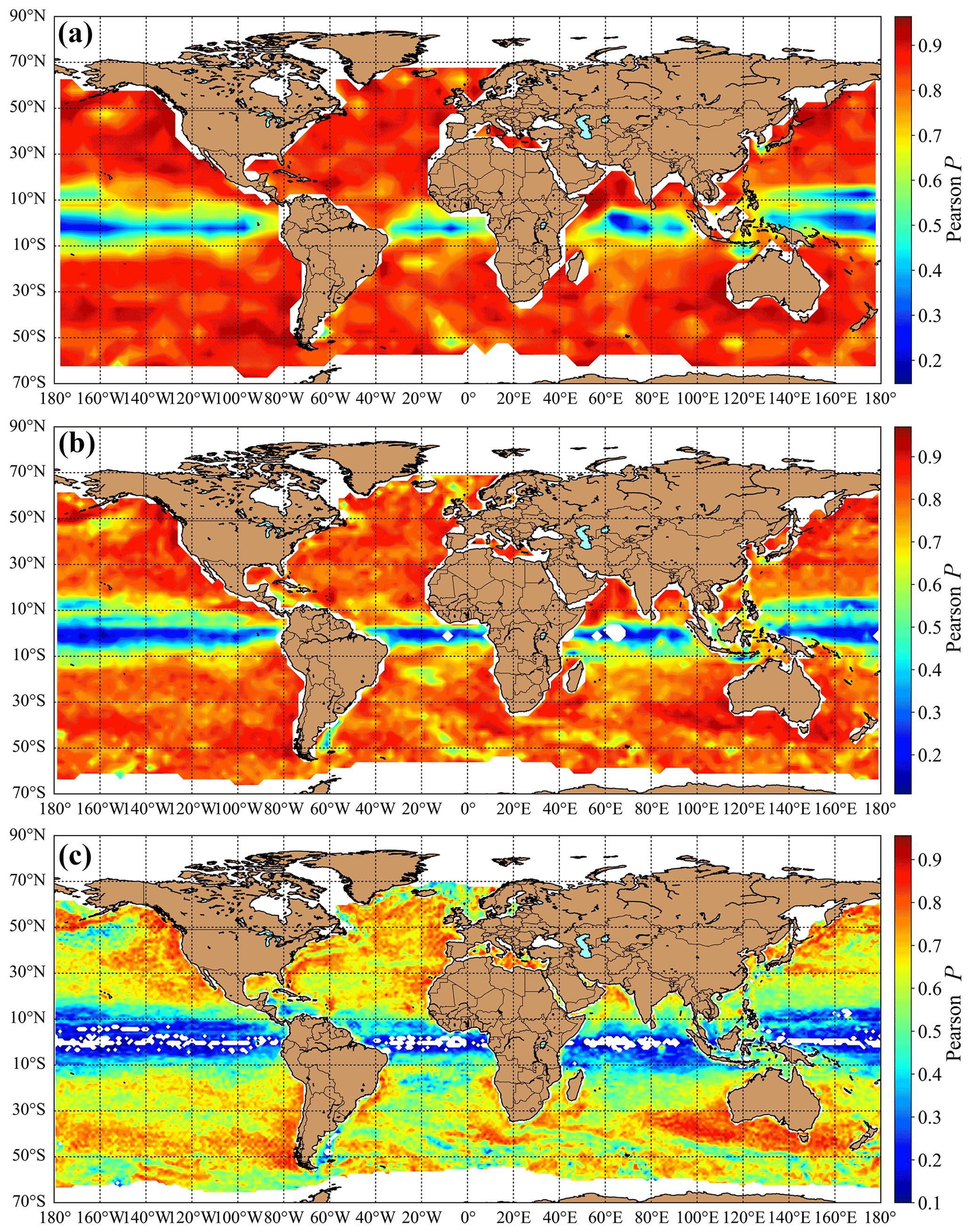
Figure 2Pearson correlation coefficients P for the integrated kinetic energy IEKE(t) and enstrophy IZ(t) at three different tilings determined for the whole period of AVISO records. (a) 21 × 21 grid cells; (b) 11 × 11 grid cells; (c) 5 × 5 grid cells (for details see Sect. 2.3).
3.1 Correlations between IEKE(t) and IZ(t), vortex radii
The geographic distribution of the Pearson correlation coefficient P for IEKE(t) and IZ(t) is shown in Fig. 2a, b, and c for the three tilings, respectively. The common feature is the strongly decreasing correlation in the latitude band 10∘ S–10∘ around the Equator. This behavior is expected because the Coriolis effect vanishes at the Equator; thus, geostrophic eddies have a very short survival time when drifting close to the zero latitude. The color coding in Fig. 2 indicates stronger correlations for larger tile sizes, which is in full agreement with the result in Jánosi et al. (2019). Somewhat surprising is the fact that strong correlations between IEKE(t) and IZ(t) appear in several ocean basins at the smallest tile size of , mostly at the eastern boundaries of the basins (south to Australia and around the Agulhas, Antarctic Circumpolar, Gulf, and Kuroshio Current). The yellowish colors dominating Fig. 2c represent lower but statistically significant correlations with P values between 0.6 and 0.7.
The strong correlations permit giving an estimate for an effective proxy vortex radius Reff with Eq. (5) as . For simplicity, we show here only the map for the finest tiling in Fig. 3, adding, however, that all three panels look very similar. Likewise, in Fig. 2, we observe anomalies in the equatorial band of 10∘ S–10∘ N as unusually large vortex sizes.
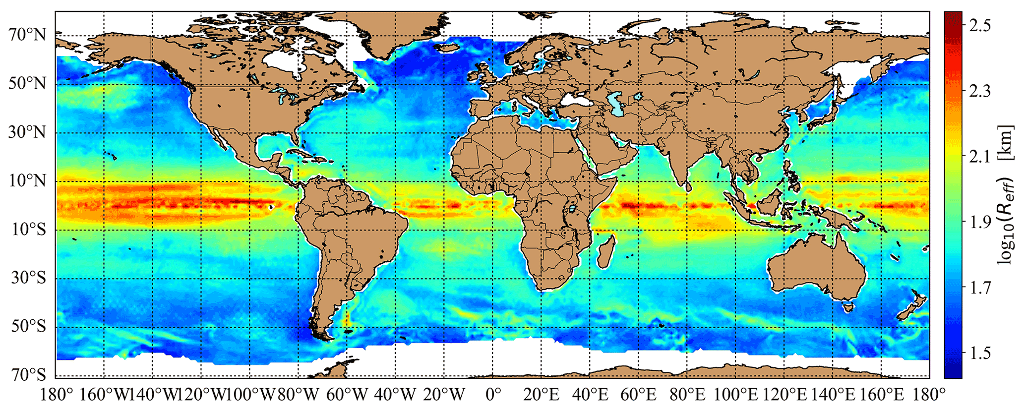
Figure 3Geographic distribution of the effective radius Reff based on the estimate by Eq. (5) for the finest tiling of . The color scale is logarithmic for better visualization. White pixels denote seasonally ice-covered regions.
For the validation of the results, Fig. 4 exhibits a comparison for five datasets. From the vortex census by Faghmous et al. (2015), we used the parameter of eddy area for each individual case because it is given in units of square kilometers (km2) and not in grid cell number; therefore, we did not need to determine the meridional corrections. We determined and plotted zonal means for an equivalent radius Requiv, which is a radius of a circular vortex of the same area as recorded. Since the identified eddies were fitted with ellipses by Faghmous et al. (2015), the lengths of the major and minor axes a and b were recorded. We checked the statistics by determining the usual parameter of eccentricity . Characteristic zonal mean values are around ϵ∼0.75 (b≈0.66a) in the large ocean basins between latitudes 40∘ S and 40∘ N. Northward and southward of this band the eccentricity gradually increases close to 1 (strongly elongated shapes). This result is in agreement with Chen et al. (2019), wherein statistics of fitted ellipses and their orientations are presented for 2.6 million individual eddies. However, a simple visual check of a couple of maps (not shown here) indicates that an ellipsoidal fit is also an approximation. Mesoscale eddies strongly interact with the neighbors, and before they decay, the isocontours of sea height anomalies exhibit rather complex features with lobes and waves around.
The agreement between the five estimates of zonal mean effective radii Reff and Requiv is rather satisfactory for the latitudinal bands 80–20∘ S and 20–80∘ N. The gray band indicates the equatorial zone where we obtained poor correlations (see Fig. 2). Despite this fact, we plotted the estimates for the following reason. The vortex data bank (Faghmous et al., 2015) contains a surprisingly large number of mesoscale eddies in this “gray zone” (see Fig. 4) with rather large equivalent radii. Since this band cannot be a source of geostrophic eddies, they must be advected here from higher and lower latitudes. These eddies have systematically low amplitudes, and therefore their detection by isocontours can have a large error and can easily result in underestimates of their size. Unfortunately, eddy radius estimates by Eq. (5) are rather unreliable in the gray zone too because of the low level of correlations at each tiling (see Fig. 2).
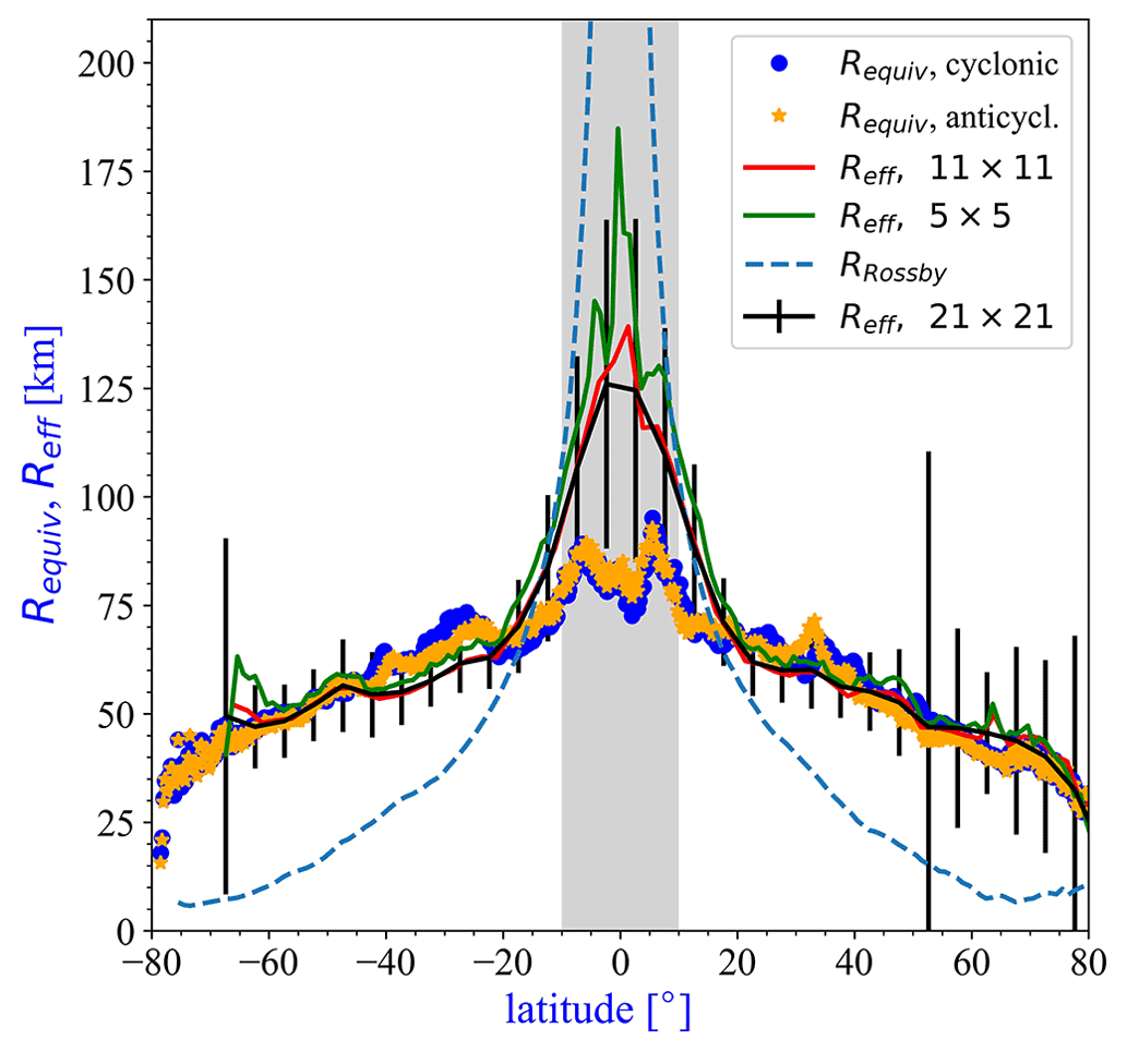
Figure 4Zonal and temporal mean values of the characteristic vortex sizes Requiv and Reff for five datasets. Solid symbols are statistics from the vortex database (Faghmous et al., 2015), with 32 million cyclonic (blue symbols) and about the same number of anticyclonic eddies (orange stars) MEs. Solid lines are the estimates by Eq. (5) for the three tilings; see legend. The gray band denotes the equatorial region of low correlations (see Fig. 1) where the estimates for Reff are particularly unreliable. Black error bars are for Reff statistics (1σ) with the largest tiles (21 × 21) of integration. For comparison, the dashed line indicates the zonal mean Rossby radius of deformation; data are from Chelton et al. (1998).
Note that averaging should be performed with care. This is due to a finite size effect: it often occurs that no eddies (more precisely, no eddy centers) are identified in a given day and in a given tile by the eddy census. Actually, from the aggregated dataset of size 7792 × 36 × 72 (days × long × lat), 26.3 % of the largest tiles and 31.1 % of the medium-sized tiles (out of 7792 × 72 × 144) are zeros. For this reason, all zero values in the tile-wise eddy census were masked, and the mask was used in all data series before computing mean values.
The dashed line in Fig. 4 denotes the mean Rossby radius of deformation (Chelton et al., 1998). It is well known that MEs usually have larger equivalent radii than the Rossby radius at a given latitude due to essential (albeit weak) nonlinearities (Matsuura and Yamagata, 1982; Roisin and Tang, 1990; Dewar and Killworth, 1995; Willett et al., 2006; Chelton et al., 2011), and it is properly reproduced in high-resolution ocean models (Ajayi et al., 2020; Moreton et al., 2020). The agreement between the proxy vortex approximation and a previous global direct vortex census by Chelton et al. (2011, see Fig. 12) is remarkably good.
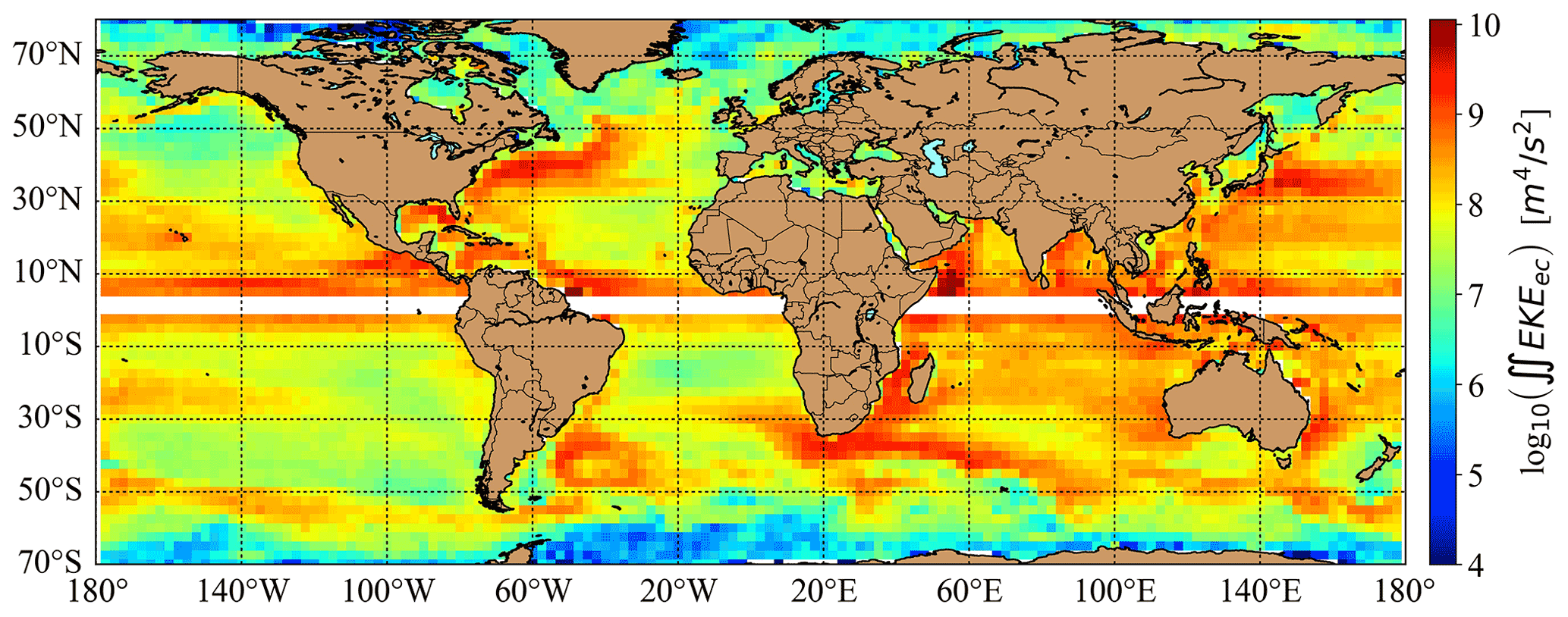
Figure 5Temporal mean eddy kinetic energy ∬EKEec estimated from the squared amplitude parameters of the eddy census by Eq. (3) for the tiling of 11 × 11 grid cells. The white band indicates the equatorial region where estimates diverge because the Coriolis parameter ∼sin (φ) in the denominator of Eq. (3) tends to zero. The color scale is logarithmic for better visualization.
3.2 Vortex amplitudes and kinetic energies
In order to compare amplitudes of proxy vortices and amplitudes (stored height parameters) in the eddy census database, one can explore Eq. (3). Since IEKE depends only on the squared peak height of a Gaussian proxy vortex (and some constants), proxy vortex amplitudes can be obtained by inserting the sum of kinetic energies belonging to identified eddies ∬EKEec in the eddy census. As described in Sect. 2.4, we performed the calculation in the reverse direction. Instead of attempting to extract sum of squared peak heights from IEKE, we estimated the eddy kinetic energy tile-wise from the eddy census ∬EKEec by inserting the stored amplitudes into Eq. (3). This approximation assumes that MEs have Gaussian sea level anomaly profiles in general. The result for temporal mean values is illustrated in Fig. 5. As expected, higher integrated EKEec values are characteristic in the vicinity of energetic ocean currents, where a large number of vortices are generated by baroclinic instabilities at the current edges (e.g., Willett et al., 2006; Smith, 2007; Badin et al., 2009; Molemaker et al., 2015; Marta and Isachsen, 2018; Pnyushkov et al., 2018).
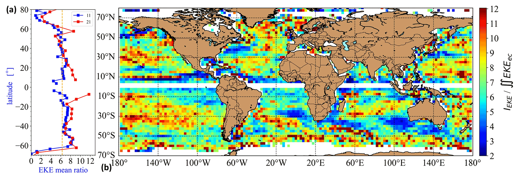
Figure 6Temporal mean eddy kinetic energy ratio . The latter estimated from the squared amplitude parameters of the eddy census by Eq. (3). (a) Zonal mean values for the tilings of 11 × 11 (blue) and 21 × 21 (red) grid cells. The vertical dashed line (orange) is not fitted and is only for orientation. (b) Geographic distribution for the tiling of 11 × 11 grid cells. The white band indicates the equatorial region where estimates diverge because the Coriolis parameter ∼sin (φ) in the denominator of Eq. (3) tends to zero. The color scale is linear.
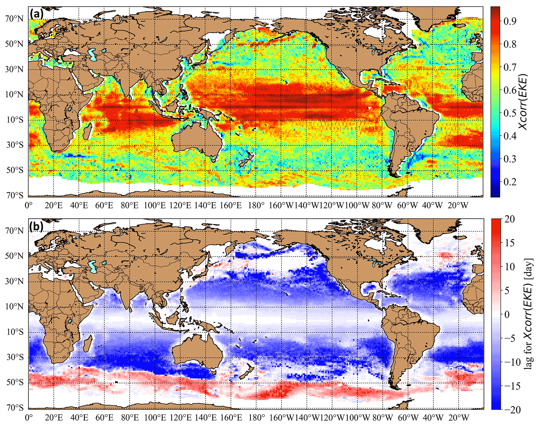
Figure 7Time-dependent cross-correlation analysis of the EKE field by Eq. (8) for the smallest tiling (5 × 5 grid cells). Only zonal neighbors are considered. The color scales are linear. (a) The level of maximal cross-correlation for each valid tile. (b) The time lag of maximal cross-correlation for each valid tile. Blueish and reddish coloring indicates dominant westward and eastward zonal drifting tendency.
Figure 6 illustrates the tile-wise mean ratio , which is equivalent with the ratio of squared amplitudes (see Eq. 3) in the Gaussian approximation. The map in Fig. 6b is rather pixelated, indicating high variabilities. Indeed, in both space and time the local values of the eddy kinetic energy ratios fluctuate strongly between 0.5 and 15. Note that, here again, only the dates were considered in the determination of mean values when at least a single eddy center was detected in a given tile. The range of mean ratios is of the same order of magnitude as found by Amores et al. (2018) (they reported a partition ratio between 1 and 5 fluctuating strongly in time); however, it differs from Fig. 5b in Jánosi et al. (2019). In the latter, a mean ratio around 2 was deduced in a restricted ocean region along the shoreline of Oregon and California. However, the way of estimating eddy heights was different. While in Jánosi et al. (2019) the values of sea level anomaly at the very center of identified eddies were used as proxies, here we directly extracted the amplitude parameters from the eddy census by Faghmous et al. (2015).
These statistics also suffer from an additional finite size effect, besides the occasional lack of identified vortices. When the location of an ME is close to the boundary of the given tile, its contribution to ∬EKEec is larger than to IEKE (determined by direct counting from geostrophic velocity anomalies []). This is because the implied integration domain in Eq. (3) is infinite for a given eddy, but only about half of it contributes to the counting of total kinetic energy inside the tile. As a consequence, in several cases the daily ratio is smaller than 1, suggesting that eddy centers in the given tile are close to the tile edges. Fortunately this bias is not too strong; at least the zonal mean values shown in Fig. 6a are consistent for the medium and largest tile sizes (far enough from the Equator).
An essential and well-known source of input data errors is the difficulty of measuring eddy amplitude from altimeter data. Most of the recorded amplitudes are small in the range of a few centimeters, and the reference level is usually the approximate height of the identified close contour (depending on the method). Small eddies (in both extent and height) are poorly resolvable at the available spatial resolutions, and therefore estimates are certainly loaded with errors. In order to check the sensitivity of the method to amplitude errors, we repeated all the calculations whereby the amplitude values are systematically shifted up by +1 cm (note that large eddies of 0.5 m or similar are hardly affected by such a shift). The results changed rather strongly: while the curves of zonal mean values keep all the presented geographic tendencies (see Fig. 6a), the partition ratio dropped to a mean value of 4.3 instead of 6.2, illustrating the sensitivity of our approach.
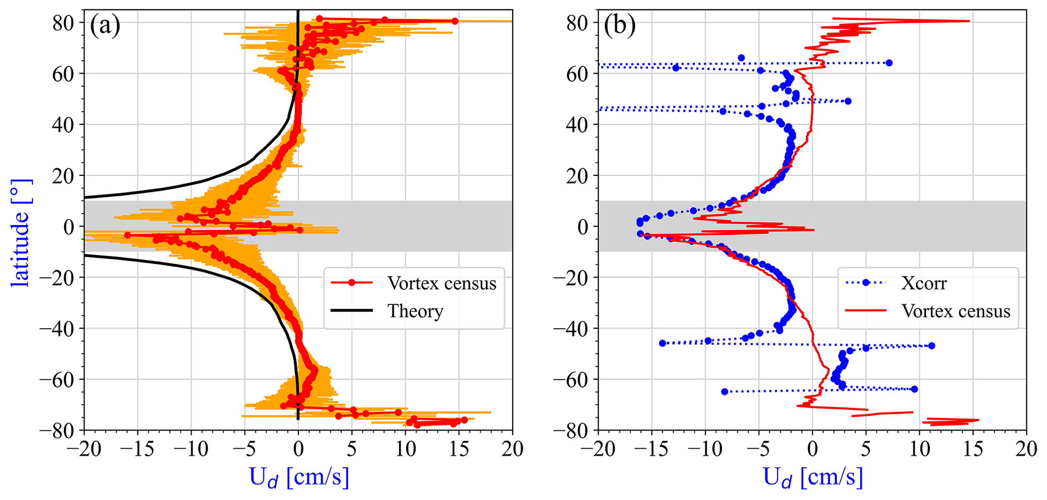
Figure 8Zonal mean values of the characteristic zonal drift speed Ud in units of centimeters per second (cm s−1) for three datasets. Gray bands emphasize the tropical region of particularly strong cross-correlation values (see Fig. 7a). (a) Red symbols (with orange error bars) indicate the result from the tracks of vortex census. The solid black line is the estimate for nondispersive Rossby waves in Eq. (7). (b) Blue symbols denote the result for the cross-correlation analysis at the smallest tiling (); anomalously low time lag values ( d) are filtered out from the statistics. The red line represents the mean drift speeds from (a).
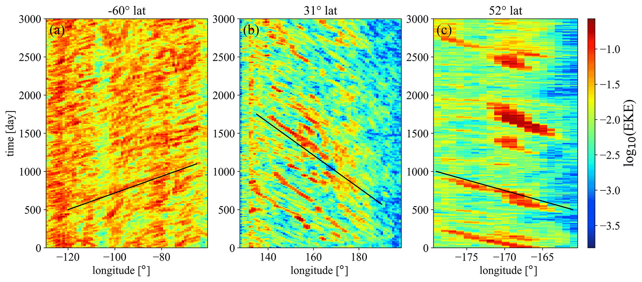
Figure 9Hovmöller plots (time–longitude diagrams) of eddy kinetic energy propagation for three particular regions. Latitudes are indicated in the title of panels. Black lines guide the eye for characteristic slopes. Color scales are logarithmic. (a) A southern Pacific section in the region of the Antarctic Circumpolar Current at the latitude 60∘ S. The eastward drift speed (black line) is estimated as 5.8 cm s−1. (b) A northern Pacific section at the latitude 31∘ N. The westward drift speed (black line) is around −5.2 cm s−1. (c) A northern Pacific section at the latitude of 52∘ N, rather close to the Fox Islands. The rare extreme energetic vortices obey a westward drift speed around −2.9 cm s−1.
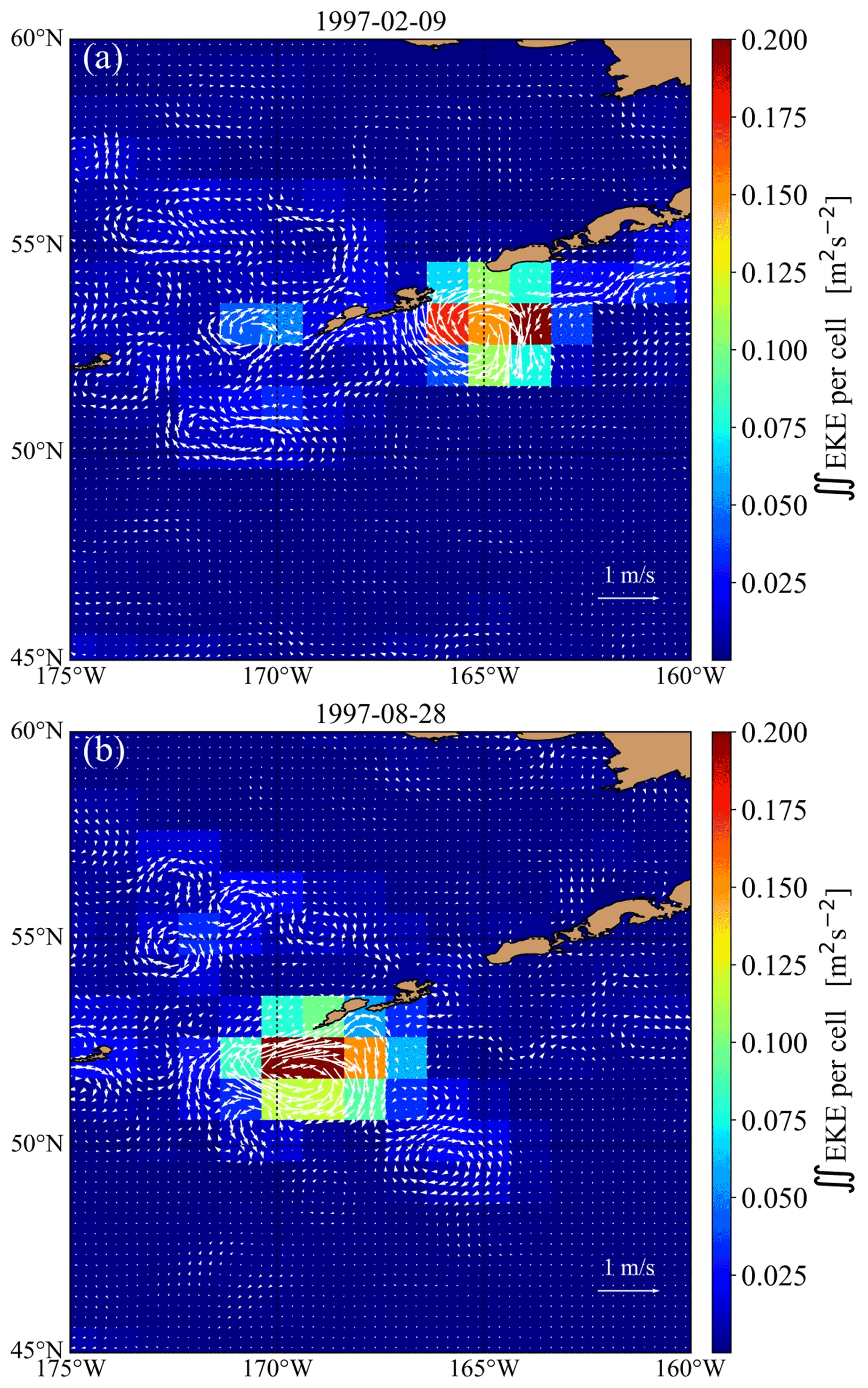
Figure 10Snapshots of the geostrophic flow field and integrated kinetic energy (color scale is linear) for two time instances in the northern Pacific region analyzed in Fig. 9c. (a) 9 February 1997 (day 1500 in Fig. 9c). (b) 200 d later on 28 August 1997 (day 1700 in Fig. 9c). The radius of the huge anticyclonic vortex has a length around 300–350 km (note that the apparent elongation is the consequence of equidistant cylindrical map projection).
3.3 Eddy drift properties
The results for the analysis of (mostly) westward drift (see Sect. 2.5) are presented in Figs. 7 and 8. The geographic distribution for the coefficient of cross-correlations (X(τ) in Eq. 8) in Fig. 7a exhibits high statistical significance almost everywhere, particularly in the band 30∘ S–30∘ N. The time lags τ at the maximum cross-correlations obey definite negative values in this band (blue in Fig. 7b), indicating marked westward drift. Eastward drift (red in Fig. 7b) is characteristic in the regions of the Antarctic Circumpolar Current as well as at the northern Gulf and Kuroshio Currents, as expected. Note the appearance of large white areas along the Equator and at larger than 40∘ latitudes on both hemispheres, indicating very short time lags of 1–2 d or even zero (recall that the temporal resolution of flow fields is 1 d). Nearly zero lags result in anomalously large values for velocity estimates as distance over time lag. By checking several flow field maps, it seems that these regions can be characterized by weak vortex activity. One plausible explanation is that lag-zero significant cross-correlations are related to simultaneous kinetic energy changes with the wind field over extended areas pumping kinetic energy into or from the oceanic surface layer.
Figure 8 illustrates the comparison of drift speed results, zonal mean values for the vortex data bank (red symbols and orange error bars, Fig. 8a), and the cross-correlation analysis (blue, Fig. 8b). The results of the cross-correlation method are in good agreement with vortex tracking statistics in the latitude bands 5–30∘ on both hemispheres. Stronger discrepancies are present in the bands 30–50∘, again on both hemispheres. As for the narrow band 5∘ S–5∘ N along the Equator, the vortex census statistics indicate a sharp drop in propagation speeds. Since here mesoscale eddies cannot survive a long time with a lack of the Coriolis effect, the statistics break down.
The observed discrepancies can be explained by the fact that mesoscale eddies are not the only form of kinetic energy transport on the ocean surfaces. We have already noted that the eddy kinetic energy field estimated from the geostrophic velocity anomalies (see Fig. 1a) has a surprisingly large contribution from the energetic current systems of apparently strong temporal and spatial variabilities. The strong and narrow eastward currents at higher latitudes are parts of the top branch of ocean gyres. This probably explains the anomalies also present in the vortex tracking statistics: particularly in the latitude bands 40–50∘ on both hemispheres, the mean propagating velocity is zero or near zero (see Fig. 8). Standing mesoscale eddies can exist only where the westward drift is balanced by an eastward background flow. Along the Equator, freely propagating, nondispersive, linear, first-mode baroclinic Rossby waves are common (Chelton and Schlax, 1996, see also Fig. 5a), suggesting that cross-correlation analysis detects such Rossby waves in this band. Furthermore, long-living MEs might be related to Rossby waves as suggested recently by Sutyrin et al. (2021). When steady propagating baroclinic vortices are embedded in a large-scale vertical shear, they can radiate Rossby waves without decay by extracting available potential energy from the vertically sheared background flow (Sutyrin et al., 2021).
3.4 Eddy kinetic energy transport
In order to further elaborate the possible reasons for the discrepancies between the drift speed values obtained by the two methods, we studied the Hovmöller diagrams (time–longitude plots) for several latitudes. Three examples are illustrated in Fig. 9. Red coloring indicates the time evolution of the locations where the eddy kinetic energy per grid cell has relatively high values. In Fig. 9a, the visible drift is eastward; this is no wonder because this region falls into the band of the Antarctic Circumpolar Current (see Fig. 7b). The pattern suggests that vortical activity is patchy and formed by small eddies of short lifetimes. The usual westward propagation pattern is illustrated in Fig. 9b. Notably, this eastern section of the North Pacific basin along 31∘ N is also interrupted by white areas of short time lags (see Fig. 7b), indicating the lack of mesoscale eddies. Even after the filtering, τ≥3 lags give anomalously large drift speed values to the zonal mean. An interesting situation is exhibited in Fig. 9c. This section along the Aleutian Islands in the northeastern Pacific is characterized by the quasi-periodic appearance of a single giant energetic eddy or ocean ring advected by the Alaskan Stream. Such an event is depicted in Fig. 10, where the huge ring of diameter 300–350 km passes by westward between day 1500 (9 February 1997) and day 2000 (24 June 1998). Similar giant rings have been known and studied mostly by satellite altimetry for a few decades (Ladd et al., 2007; Ueno et al., 2009; Lyman and Johnson, 2015; Prants et al., 2019). Recent results suggest that their unusually long lifetime is related to the bottom topography (Gulliver and Radko, 2022).
Since we already discussed the results in the subsections above, here we list the main findings of this work.
-
The eddy kinetic energy (EKE) obtained from the 2D geostrophic velocity anomalies [] of the AVISO data bank partly reflects the activity of mesoscale eddies; however, it has significant contributions from the meandering and swinging of the major western boundary and equatorial currents (see Fig. 1).
-
The time-dependent integrated eddy kinetic energy IEKE and integrated enstrophy IZ are strongly correlated except along the Equator. The larger the area of integration the stronger the temporal Pearson correlation (see Fig. 2). While there is no correlation in a single grid cell of size with a single mean velocity (assigned to the center of grid cells), and integration area of 5×5 grid cells () is enough to exhibit significant correlations almost everywhere (see Fig. 2c).
-
The effective zonal mean radii of proxy vortices Reff obtained by Eq. (5) are in good agreement with zonal mean values extracted from the eddy census by Faghmous et al. (2015) away from the equatorial band 10∘S, 10∘ N (see Fig. 4). Here correlations between IEKE and IZ are decaying, and thus the approximation by Eq. (5) breaks down.
-
Integrated eddy kinetic energies are obtained by two estimates. Firstly, IEKE is computed from geostrophic velocity anomalies by direct counting. Secondly, for an approximation of the “true” eddy contribution ∬EKEec, squared amplitudes from the eddy census by Faghmous et al. (2015) are inserted into Eq. (3). The zonal mean ratio of is somewhat larger than found in previous analyses (see Fig. 6a); however, this ratio is very sensitive to small errors in recorded eddy amplitudes. A uniform upward shift by 1 cm resulted in a ∼30 % drop in zonal mean values.
-
As for the propagation of kinetic energy and drift of eddies, the estimates from time-lagged cross-correlation analysis of EKE fields are in general agreement with vortex tracking statistics considering order of magnitude and sign (see Fig. 8). However, it provides somewhat larger drift velocities than that of individual mesoscale eddies. Discrepancies are not unexpected because, besides mesoscale eddies, Rossby wave activities, coherent currents, and other propagating features on the ocean surface apparently contribute to the zonal transport of kinetic energy.
We can shortly conclude that the original proposal by Jánosi et al. (2019) works on a global scale. The comparison with the rich eddy census database by Faghmous et al. (2015) resulted in good agreement in many aspects, validating the Gaussian proxy vortex approach. Apparent discrepancies also provide useful insight, e.g., into the separation of kinetic energy between “true” eddy and background flow contributions or into the mechanisms of kinetic energy transport.
Global geostrophic velocity fields are openly available after registration at the EU Copernicus Marine Service (https://resources.marine.copernicus.eu/products, Taburet et al., 2019). The mesoscale vortex data bank assembled by Faghmous et al. (2015) is available at https://doi.org/10.5061/dryad.gp40h (Faghmous et al., 2016), together with MATLAB routines in the Zenodo source code repository (https://doi.org/10.5281/zenodo.13037, Faghmous et al., 2014). All the other calculations and plotting are based on standard Python modules described in Sect. 2 (“Data and methods” section) in detail.
IMJ designed the research. IMJ and MV performed the research. HK and JACG contributed new numerical and analytical tools. IMJ and HK analyzed data. IMJ, HK, JACG, and MV wrote the paper.
The contact author has declared that none of the authors has any competing interests.
Publisher's note: Copernicus Publications remains neutral with regard to jurisdictional claims in published maps and institutional affiliations.
This work was supported by the Hungarian National Research, Development and Innovation Office under grant numbers FK-125024 and K-125171, as well as by the Visitor Programme of Max Planck Institute for the Physics of Complex Systems. Jason A. C. Gallas was supported by CNPq, Brazil, under grant PQ-305305/2020-4.
This research has been supported by the Max-Planck-Institut für Physik Komplexer Systeme (Visitor Programme), the Nemzeti Kutatási Fejlesztési és Innovációs Hivatal, National Research, Development and Innovation Office (grant nos. FK-125024 and K-125171), and the Conselho Nacional de Desenvolvimento Científico e Tecnológico, Ciência sem Fronteiras (grant no. PQ-305305/2020-4).
The article processing charges for this open-access publication were covered by the Max Planck Society.
This paper was edited by Ilker Fer and reviewed by Takaya Uchida and one anonymous referee.
Ajayi, A., Le Sommer, J., Chassignet, E., Molines, J.-M., Xu, X., Albert, A., and Cosme, E.: Spatial and temporal variability of the North Atlantic eddy field from two kilometric-resolution ocean models, J. Geophys. Res.-Ocean, 125, e2019JC015827, https://doi.org/10.1029/2019JC015827, 2020. a
Amores, A., Jordà, G., Arsouze, T., and Le Sommer, J.: Up to what extent can we characterize ocean eddies using present-day gridded altimetric products?, J. Geophys. Res.-Ocean., 123, 7220–7236, https://doi.org/10.1029/2018JC014140, 2018. a, b
Aviso: Altimetry products were processed by SSALTO/DUACS and distributed by AVISO+ with support from CNES, https://www.aviso.altimetry.fr, last access: 12 September 2022, 1993–2018. a, b, c
Badin, G., Williams, R. G., Holt, J. T., and Fernand, L. J.: Are mesoscale eddies in shelf seas formed by baroclinic instability of tidal fronts?, J. Geophys. Res.-Ocean., 114, C005340, https://doi.org/10.1029/2009JC005340, 2009. a, b
Beron-Vera, F. J., Hadjighasem, A., Xia, Q., Olascoaga, M. J., and Haller, G.: Coherent Lagrangian swirls among submesoscale motions, P. Natl. Acad. Sci. USA, 116, 18251–18256, https://doi.org/10.1073/pnas.1701392115, 2018. a
Brach, L., Deixonne, P., Bernard, M.-F., Durand, E., Desjean, M.-C., Perez, E., van Sebille, E., and ter Halle, A.: Anticyclonic eddies increase accumulation of microplastic in the North Atlantic subtropical gyre, Mar. Pollut. Bull., 126, 191–196, https://doi.org/10.1016/j.marpolbul.2017.10.077, 2018. a, b
Carton, X. and Mcwilliams, J.: Barotropic and baroclinic instabilities of axisymmetric vortices in a quasigeostrophic model, in: Mesoscale/Synoptic Coherent structures in Geophysical Turbulence, edited by: Nihoul, J. and Jamart, B., Vol. 50, Elsevier Oceanography Series, 225–244, Elsevier, https://doi.org/10.1016/S0422-9894(08)70188-0, 1989. a
Cetina-Heredia, P., Roughan, M., van Sebille, E., Keating, S., and Brassington, G. B.: Retention and leakage of water by mesoscale eddies in the East Australian Current System, J. Geophys. Res.-Ocean., 124, 2485–2500, https://doi.org/10.1029/2018JC014482, 2019. a, b
Chelton, D. B. and Schlax, M. G.: Global observations of oceanic Rossby waves, Science, 272, 234–238, https://doi.org/10.1126/science.272.5259.234, 1996. a
Chelton, D. B., deSzoeke, R. A., Schlax, M. G., Naggar, K. E., and Siwertz, N.: Geographical variability of the first-baroclinic Rossby radius of deformation, J. Phys. Oceanogr., 28, 433–460, https://doi.org/10.1175/1520-0485(1998)028<0433:GVOTFB>2.0.CO;2, 1998. a, b, c
Chelton, D. B., Schlax, M. G., Samelson, R. M., and de Szoeke, R. A.: Global observations of large oceanic eddies, Geophys. Res. Lett., 34, L15606, https://doi.org/10.1029/2007GL030812, 2007. a, b, c, d
Chelton, D. B., Schlax, M. G., and Samelson, R. M.: Global observations of nonlinear mesoscale eddies, Prog. Oceanogr., 91, 167–216, https://doi.org/10.1016/j.pocean.2011.01.002, 2011. a, b, c, d, e, f, g
Chen, G., Han, G., and Yang, X.: On the intrinsic shape of oceanic eddies derived from satellite altimetry, Remote Sens. Environ., 228, 75–89, https://doi.org/10.1016/j.rse.2019.04.011, 2019. a
Chérubin, L. M., Paih, N. L., and Carton, X. J.: Submesoscale instability in the Straits of Florida, J. Phys. Oceanogr., 51, 2599–2615, https://doi.org/10.1175/JPO-D-20-0283.1, 2021. a
Cotter, C. H.: Sines, versines and haversines in nautical astronomy, J. Navig., 27, 536––541, https://doi.org/10.1017/S0373463300029337, 1974. a
Cushman-Roisin, B., Tang, B., and Chassignet, E. P.: Westward motion of mesoscale eddies, J. Phys. Oceanogr., 20, 758–768, https://doi.org/10.1175/1520-0485(1990)020<0758:WMOME>2.0.CO;2, 1990. a, b
Dewar, W. K. and Killworth, P. D.: On the stability of oceanic rings, J. Phys. Oceanogr., 25, 1467–1487, https://doi.org/10.1175/1520-0485(1995)025<1467:OTSOOR>2.0.CO;2, 1995. a
Drótos, G. and Tél, T.: On the validity of the β-plane approximation in the dynamics and the chaotic advection of a point vortex pair model on a rotating sphere, J. Atmos. Sci., 72, 415–429, https://doi.org/10.1175/JAS-D-14-0101.1, 2015. a
Early, J. J., Samelson, R. M., and Chelton, D. B.: The evolution and propagation of quasigeostrophic ocean eddies, J. Phys. Oceanogr., 41, 1535–1555, https://doi.org/10.1175/2011JPO4601.1, 2011. a, b
El Aouni, A.: A hybrid identification and tracking of Lagrangian mesoscale eddies, Phys. Fluids, 33, 036604, https://doi.org/10.1063/5.0038761, 2021. a
Escudier, R., Renault, L., Pascual, A., Brasseur, P., Chelton, D., and Beuvier, J.: Eddy properties in the Western Mediterranean Sea from satellite altimetry and a numerical simulation, J. Geophys. Res.-Ocean., 121, 3990–4006, https://doi.org/10.1002/2015JC011371, 2016. a
Faghmous, J. H., Uluyol, M., Warmka, R., Ngyuen, H., Yao, Y., and Lindell, A.: A Daily Global Mesoscale Ocean Eddy Dataset From Satellite Altimetry (v1.1), Zenodo [data set], https://doi.org/10.5281/zenodo.13037, 2014. a
Faghmous, J., Frenger, I., Yao, Y., R. Warmka, R., Lindell, A., and Kumar, V.: A daily global mesoscale ocean eddy dataset from satellite altimetry, Sci. Data, 2, 150028, https://doi.org/10.1038/sdata.2015.28, 2015. a, b, c, d, e, f, g, h, i, j, k, l, m, n, o
Faghmous, J. H., Frenger, I., Yao, Y., Warmka, R., Lindell, A., and Kumar, V.: Data from: A daily global mesoscale ocean eddy dataset from satellite altimetry, Dryad [data set], https://doi.org/10.5061/dryad.gp40h, 2016. a
Frenger, I., Münnich, M., Gruber, N., and Knutti, R.: Southern Ocean eddy phenomenology, J. Geophys. Res.-Ocean., 120, 7413–7449, https://doi.org/10.1002/2015JC011047, 2015. a
Gulliver, L. T. and Radko, T.: Topographic stabilization of ocean rings, Geophys. Res. Lett., 49, e2021GL097686, https://doi.org/10.1029/2021GL097686, 2022. a
Haller, G.: Lagrangian coherent structures, Annu. Rev. Fluid Mech., 47, 137–162, https://doi.org/10.1146/annurev-fluid-010313-141322, 2015. a
Haller, G., Karrasch, D., and Kogelbauer, F.: Material barriers to diffusive and stochastic transport, P. Natl. Acad. Sci. USA, 115, 9074–9079, https://doi.org/10.1073/pnas.1720177115, 2018. a
Harris, C. R., Millman, K. J., van der Walt, S. J., Gommers, R., Virtanen, P., Cournapeau, D., Wieser, E., Taylor, J., Berg, S., Smith, N. J., Kern, R., Picus, M., Hoyer, S., van Kerkwijk, M. H., Brett, M., Haldane, A., del Río, J. F., Wiebe, M., Peterson, P., Gérard-Marchant, P., Sheppard, K., Reddy, T., Weckesser, W., Abbasi, H., Gohlke, C., and Oliphant, T. E.: Array programming with NumPy, Nature, 585, 357–362, https://doi.org/10.1038/s41586-020-2649-2, 2020. a
Hopfinger, E. J. and van Heijst, G. J. F.: Vortices in rotating fluids, Annu. Rev. Fluid Mech., 25, 241–289, https://doi.org/10.1146/annurev.fl.25.010193.001325, 1993. a, b
Jánosi, I. M., Vincze, M., Tóth, G., and Gallas, J. A. C.: Single super-vortex as a proxy for ocean surface flow fields, Ocean Sci., 15, 941–949, https://doi.org/10.5194/os-15-941-2019, 2019. a, b, c, d, e, f, g, h, i
Ji, J., Dong, C., Zhang, B., Liu, Y., Zou, B., King, G. P., Xu, G., and Chen, D.: Oceanic eddy characteristics and generation mechanisms in the Kuroshio Extension region, J. Geophys. Res.-Ocean., 123, 8548–8567, https://doi.org/10.1029/2018JC014196, 2018. a, b
Keppler, L., Cravatte, S., Chaigneau, A., Pegliasco, C., Gourdeau, L., and Singh, A.: Observed characteristics and vertical structure of mesoscale eddies in the Southwest Tropical Pacific, J. Geophys. Res.-Ocean., 123, 2731–2756, https://doi.org/10.1002/2017JC013712, 2018. a
Kurian, J., Colas, F., Capet, X., McWilliams, J. C., and Chelton, D. B.: Eddy properties in the California Current System, J. Geophys. Res., 116, C08027, https://doi.org/10.1029/2010JC006895, 2011. a, b
Ladd, C., Mordy, C. W., Kachel, N. B., and Stabeno, P. J.: Northern Gulf of Alaska eddies and associated anomalies, Deep-Sea Res. Pt. I., 54, 487–509, https://doi.org/10.1016/j.dsr.2007.01.006, 2007. a
Li, Q.-Y., Sun, L., and Lin, S.-F.: GEM: a dynamic tracking model for mesoscale eddies in the ocean, Ocean Sci., 12, 1249–1267, https://doi.org/10.5194/os-12-1249-2016, 2016. a
Lyman, J. M. and Johnson, G. C.: Anomalous eddy heat and freshwater transport in the Gulf of Alaska, J. Geophys. Res.-Ocean., 120, 1397–1408, https://doi.org/10.1002/2014JC010252, 2015. a
Marta, T. and Isachsen, P. E.: Topographic influence on baroclinic instability and the mesoscale eddy field in the northern North Atlantic Ocean and the Nordic Seas, J. Phys. Oceanogr., 48, 2593–2607, https://doi.org/10.1175/JPO-D-17-0220.1, 2018. a, b
Martínez-Moreno, J., Hogg, A. M., Kiss, A. E., Constantinou, N. C., and Morrison, A. K.: Kinetic energy of eddy-like features from sea surface altimetry, J. Adv. Model. Earth Syst., 11, 3090–3105, https://doi.org/10.1029/2019MS001769, 2019. a, b, c
Martínez-Moreno, J., Hogg, A., England, M., Constantinou, N. C., Kiss, A. E., and Morrison, A. K.: Global changes in oceanic mesoscale currents over the satellite altimetry record, Nat. Clim. Change, 11, 397–403, https://doi.org/10.1038/s41558-021-01006-9, 2021. a
Mason, E., Pascual, A., and McWilliams, J. C.: A new sea surface height–based code for oceanic mesoscale eddy tracking, J. Atmos. Oceanic Technol., 31, 1181–1188, https://doi.org/10.1175/JTECH-D-14-00019.1, 2014. a
Matsuura, T. and Yamagata, T.: On the evolution of nonlinear planetary eddies larger than the radius of deformation, J. Phys. Oceanogr., 12, 440–456, https://doi.org/10.1175/1520-0485(1982)012<0440:OTEONP>2.0.CO;2, 1982. a
Molemaker, M. J., McWilliams, J. C., and Dewar, W. K.: Submesoscale instability and generation of mesoscale anticyclones near a separation of the California Undercurrent, J. Phys. Oceanogr., 45, 613–629, https://doi.org/10.1175/JPO-D-13-0225.1, 2015. a
Moreton, S. M., Ferreira, D., Roberts, M. J., and Hewitt, H. T.: Evaluating surface eddy properties in coupled climate simulations with “eddy-present” and “eddy-rich” ocean resolution, Ocean Model., 147, 101567, https://doi.org/10.1016/j.ocemod.2020.101567, 2020. a
Nencioli, F., Dong, C., Dickey, T., Washburn, L., and McWilliams, J. C.: A vector geometry–based eddy detection algorithm and its application to a high-resolution numerical model product and high-frequency radar surface velocities in the Southern California Bight, J. Atmos. Ocean. Technol., 27, 564–579, https://doi.org/10.1175/2009JTECHO725.1, 2010. a
Nurser, A. J. G. and Bacon, S.: The Rossby radius in the Arctic Ocean, Ocean Sci., 10, 967–975, https://doi.org/10.5194/os-10-967-2014, 2014. a
Pegliasco, C., Delepoulle, A., Mason, E., Morrow, R., Faugère, Y., and Dibarboure, G.: META3.1exp: a new global mesoscale eddy trajectory atlas derived from altimetry, Earth Syst. Sci. Data, 14, 1087–1107, https://doi.org/10.5194/essd-14-1087-2022, 2022. a
Pessini, F., Olita, A., Cotroneo, Y., and Perilli, A.: Mesoscale eddies in the Algerian Basin: do they differ as a function of their formation site?, Ocean Sci., 14, 669–688, https://doi.org/10.5194/os-14-669-2018, 2018. a, b
Pnyushkov, A., Polyakov, I. V., Padman, L., and Nguyen, A. T.: Structure and dynamics of mesoscale eddies over the Laptev Sea continental slope in the Arctic Ocean, Ocean Sci., 14, 1329–1347, https://doi.org/10.5194/os-14-1329-2018, 2018. a, b, c
Prants, S., Andreev, A., Uleysky, M. Y., and Budyansky, M.: Lagrangian study of mesoscale circulation in the Alaskan Stream area and the eastern Bering Sea, Deep-Sea Res. Pt. II, 169/170, 104560, https://doi.org/10.1016/j.dsr2.2019.03.005, 2019. a
Rai, S., Hecht, M., Maltrud, M., and Aluie, H.: Scale of oceanic eddy killing by wind from global satellite observations, Sci. Adv., 7, eabf4920, https://doi.org/10.1126/sciadv.abf4920, 2021. a
Raj, R. P., Johannessen, J. A., Eldevik, T., Nilsen, J. E. O., and Halo, I.: Quantifying mesoscale eddies in the Lofoten Basin, J. Geophys. Res.-Ocean., 121, 4503–4521, https://doi.org/10.1002/2016JC011637, 2016. a
Roisin, B. C. and Tang, B.: Geostrophic turbulence and emergence of eddies beyond the radius of deformation, J. Phys. Oceanogr., 20, 97–113, https://doi.org/10.1175/1520-0485(1990)020<0097:GTAEOE>2.0.CO;2, 1990. a
Rubio, A., Blanke, B., Speich, S., Grima, N., and Roy, C.: Mesoscale eddy activity in the southern Benguela upwelling system from satellite altimetry and model data, Progr. Oceanogr., 83, 288–295, https://doi.org/10.1016/j.pocean.2009.07.029, 2009. a
Ryzhov, E. and Berloff, P.: On transport tensor of dynamically unresolved oceanic mesoscale eddies, J. Fluid Mech., 939, A7, https://doi.org/10.1017/jfm.2022.169, 2022. a
Schütte, F., Brandt, P., and Karstensen, J.: Occurrence and characteristics of mesoscale eddies in the tropical northeastern Atlantic Ocean, Ocean Sci., 12, 663–685, https://doi.org/10.5194/os-12-663-2016, 2016. a, b
Smith, K. S.: The geography of linear baroclinic instability in Earth's oceans, J. Mar. Res., 65, 655–683, https://doi.org/10.1357/002224007783649484, 2007. a, b
Souza, J. M. A. C., de Boyer Montégut, C., and Le Traon, P. Y.: Comparison between three implementations of automatic identification algorithms for the quantification and characterization of mesoscale eddies in the South Atlantic Ocean, Ocean Sci., 7, 317–334, https://doi.org/10.5194/os-7-317-2011, 2011. a
Stammer, D.: Global Characteristics of Ocean Variability Estimated from Regional TOPEX/POSEIDON Altimeter Measurements, J. Phys. Oceanogr., 27, 1743–1769, https://doi.org/10.1175/1520-0485(1997)027<1743:GCOOVE>2.0.CO;2, 1997. a
Stammer, D. and Cazenave, A.: Satellite Altimetry Over Oceans and Land Surfaces, Earth Observation of Global Changes, CRC Press, ISBN 9780367874841, 2017. a
Sutyrin, G. G., Radko, T., and Nycander, J.: Steady radiating baroclinic vortices in vertically sheared flows, Phys. Fluids, 33, 031705, https://doi.org/10.1063/5.0040298, 2021. a, b
Taburet, G., Sanchez-Roman, A., Ballarotta, M., Pujol, M.-I., Legeais, J.-F., Fournier, F., Faugere, Y., and Dibarboure, G.: DUACS DT2018: 25 years of reprocessed sea level altimetry products, Ocean Sci., 15, 1207–1224, https://doi.org/10.5194/os-15-1207-2019, 2019 (data available at: https://resources.marine.copernicus.eu/products, last access: 13 September 2022, registration required). a, b, c, d
Tian, F., Wu, D., Yuan, L., and Chen, G.: Impacts of the efficiencies of identification and tracking algorithms on the statistical properties of global mesoscale eddies using merged altimeter data, Int. J. Remote Sens., 41, 2835–2860, https://doi.org/10.1080/01431161.2019.1694724, 2020. a
Ubelmann, C. and Fu, L.-L.: Vorticity structures in the Tropical Pacific from a numerical simulation, J. Phys. Oceanogr., 41, 1455–1464, https://doi.org/10.1175/2011JPO4507.1, 2011. a
Ueno, H., Sato, K., Freeland, H. J., Crawford, W. R., Onishi, H., Oka, E., and Suga, T.: Anticyclonic eddies in the Alaskan Stream, J. Phys. Oceanogr., 39, 934–951, https://doi.org/10.1175/2008JPO3948.1, 2009. a
van Sebille, E., Aliani, S., Law, K. L., Maximenko, N., Alsina, J. M., Bagaev, A., Bergmann, M., Chapron, B., Chubarenko, I., Cózar, A., Delandmeter, P., Egger, M., Fox-Kemper, B., Garaba, S. P., Goddijn-Murphy, L., Hardesty, B. D., Hoffman, M. J., Isobe, A., Jongedijk, C. E., Kaandorp, M. L. A., Khatmullina, L., Koelmans, A. A., Kukulka, T., Laufkötter, C., Lebreton, L., Lobelle, D., Maes, C., Martinez-Vicente, V., Maqueda, M. A. M., Poulain-Zarcos, M., Rodríguez, E., Ryan, P. G., Shanks, A. L., Shim, W. J., Suaria, G., Thiel, M., van den Bremer, T. S., and Wichmann, D.: The physical oceanography of the transport of floating marine debris, Environ. Res. Lett., 15, 023003, https://doi.org/10.1088/1748-9326/ab6d7d, 2020. a, b
Virtanen, P., Gommers, R., Oliphant, T. E., Haberland, M., Reddy, T., Cournapeau, D., Burovski, E., Peterson, P., Weckesser, W., Bright, J., van der Walt, S. J., Brett, M., Wilson, J., Millman, K. J., Mayorov, N., Nelson, A. R. J., Jones, E., Kern, R., Larson, E., Carey, C. J., Polat, İ., Feng, Y., Moore, E. W., VanderPlas, J., Laxalde, D., Perktold, J., Cimrman, R., Henriksen, I., Quintero, E. A., Harris, C. R., Archibald, A. M., Ribeiro, A. H., Pedregosa, F., van Mulbregt, P., and SciPy 1.0 Contributors: SciPy 1.0: Fundamental algorithms for scientific computing in Python, Nat. Method., 17, 261–272, https://doi.org/10.1038/s41592-019-0686-2, 2020. a
Wang, Z., Li, Q., Sun, L., Li, S., Yang, Y., and Liu, S.: The most typical shape of oceanic mesoscale eddies from global satellite sea level observations, Front. Earth Sci., 9, 202–208, https://doi.org/10.1007/s11707-014-0478-z, 2015. a
Wichmann, D., Kehl, C., Dijkstra, H. A., and van Sebille, E.: Ordering of trajectories reveals hierarchical finite-time coherent sets in Lagrangian particle data: detecting Agulhas rings in the South Atlantic Ocean, Nonlin. Processes Geophys., 28, 43–59, https://doi.org/10.5194/npg-28-43-2021, 2021. a, b
Willett, C. S., Leben, R. R., and Lavín, M. F.: Eddies and tropical instability waves in the eastern tropical Pacific: A review, Prog. Oceanogr., 69, 218–238, https://doi.org/10.1016/j.pocean.2006.03.010, 2006. a, b, c
Wunsch, C.: The oceanic variability spectrum and transport trends, Atmos.-Ocean, 47, 281–291, https://doi.org/10.3137/OC310.2009, 2009. a
Wunsch, C.: Baroclinic motions and energetics as measured by altimeters, J. Atmos. Oc. Technol., 30, 140–150, https://doi.org/10.1175/JTECH-D-12-00035.1, 2013. a
Wunsch, C. and Ferrari, R.: Vertical mixing, energy, and the general circulation of the oceans, Annu. Rev. Fluid Mech., 36, 281–314, https://doi.org/10.1146/annurev.fluid.36.050802.122121, 2004. a
Zhang, Z., Zhang, Y., Wang, W., and Huang, R. X.: Universal structure of mesoscale eddies in the ocean, Geophys. Res. Lett., 40, 3677–3681, https://doi.org/10.1002/grl.50736, 2013. a
Zhibing, L., Zhongya, C., Zhiqiang, L., Xiaohua, W., and Jianyu, H.: A novel identification method for unrevealed mesoscale eddies with transient and weak features-Capricorn Eddies as an example, Remote Sens. Environ., 274, 112981, https://doi.org/10.1016/j.rse.2022.112981, 2022. a