On the uncertainty associated with detecting global and local mean sea level drifts on Sentinel-3A and Sentinel-3B altimetry missions

An instrumental drift in the point target response (PTR) parameters has been detected on the Copernicus Sentinel-3A altimetry mission. It will affect the accuracy of sea level sensing, which could result in errors in sea level change estimates of a few tenths of a millimeter per year. In order to accurately evaluate this drift, a method for detecting global and regional mean sea level relative drifts between two altimetry missions is implemented. Associated uncertainties are also accurately calculated thanks to a detailed error budget analysis. A drift on both Sentinel-3A (S3A) and Sentinel-3B (S3B) global mean sea level (GMSL) is detected with values significantly higher than expected. For S3A, the relative GMSL drift detected is 1.0 mm yr⁻¹ with Jason-3 and 1.3 mm yr⁻¹ with SARAL/AltiKa. For S3B, the relative GMSL drift detected is −3.4 mm yr⁻¹ with Jason-3 and −2.2 mm yr⁻¹ with SARAL/AltiKa. The drift detected at global level does not show detectable regional variations above the uncertainty level of the proposed method. The investigations led by the altimeter experts can now explain the origin of this drift for S3A and S3B. The ability of the implemented method to detect a sea level drift with respect to the length of the common period is also analyzed. We find that the minimum detectable sea level drift over a 5-year period is 0.3 mm yr⁻¹ at the global scale and 1.5 mm yr⁻¹ at the 2400 km regional scale. However, these levels of uncertainty do not meet the sea level stability requirements for climate change studies.

1 Introduction

Sea level is one of the key records of climate change, integrating the changes of mass in the ocean from land-based ice melt, changes in temperature of the ocean from the excess heat entering the Earth system (Meyssignac et al., 2019; von Schuckmann et al., 2020), and changes in land water storage (Chambers et al., 2017). As such, the global mean sea level (GMSL) has been defined by the Global Climate Observing System (GCOS) as an essential climate variable (ECV). The GMSL rise is a widely accepted indicator of the current climate state (Meyssignac et al., 2019) and the GMSL acceleration for the rate at which the climate is changing.

Since 1993, the GMSL indicator has been calculated on a continual basis from four reference altimetry missions (TOPEX/Poseidon (T/P), Jason-1, Jason-2, and Jason-3), all on the same orbit. The GMSL time series of each altimeter have been accurately linked together through inter-calibration during the tandem phases (Zawadzki and Ablain, 2016): T/P–Jason-1, Jason-1–Jason-2, and Jason-3–Jason-2. The satellites follow each other very closely throughout these phases and therefore measure the water surface height with nearly identical oceanic and atmospheric conditions. The description of the errors and the uncertainties in the long-term stability of the sea level estimate for these products were provided by Ablain et al. (2019) and Prandi et al. (2021) for the global and regional scales, respectively. Over the whole altimetry period (January 1993–December 2020), the GMSL shows a significant rise of +3.48 ± 0.35 mm yr⁻¹. Rates of sea level rise vary spatially in the range 0 to 6 mm yr⁻¹, with uncertainties ranging from ±0.8 to ±1.2 mm yr⁻¹, indicating that the sea level is rising almost everywhere over the globe. Recent studies also showed that sea level is accelerating at 0.12 ± 0.07 mm yr⁻² at the global scale (Ablain et al., 2019) and ranges between −1 and +1 mm yr⁻² at the regional scale (Prandi et al., 2021). The Sentinel-6 Michael Freilich (S6-MF) mission, recently launched in November 2020 on the same historical T/P-Jason orbit, will allow the GMSL time series to be extended once the current validation phase is completed (early 2022).

Several other altimetry missions (e.g., ERS-1, ERS-2, Envisat, CryoSat-2, SARAL-AltiKa) have also been launched from 1991 onwards, all in different orbits at lower altitudes and with a longer revisit period (e.g., 35 d for Envisat). Although these missions were not designed to be as stable as T/P, Jasons, and S6-MF, their data are nevertheless very relevant to improve and verify the long-term stability of the climate altimeter record. On the one hand, data from these complementary missions combined with data from the reference climate missions can generate value-added products with higher spatiotemporal resolution and better global coverage towards the poles (e.g., sea level products from CMEMS, Taburet et al., 2019; and Copernicus Climate Change Service (C3S), Legeais et al., 2021). On the other hand, cross-comparison of complementary and reference altimetry missions over the same period allows for verification of the coherence of sea level measurements between these missions and possibly detection of relative drifts between them (e.g., Envisat GMSL drift, Ollivier et al., 2012).

More recently, the Sentinel-3A (S3A) and Sentinel-3B (S3B) altimetry missions, developed in the framework of the European Space Agency (ESA) Copernicus program, were launched in February 2016 and April 2018 to provide sea level measurements for Copernicus operational services (e.g., CMEMS, C3S). They complete the existing constellation of altimeter satellites based on Jason-2, Jason-3, and SARAL/AltiKa, to which must be added the CryoSat-2 and HY-2A/2B missions. S3A and S3B are equipped with a synthetic-aperture radar (SAR)/Doppler altimeter instead of a conventional altimeter like the climate reference missions. This new altimeter has a much better along-track resolution, and its measurements are very accurate. However, this mission is not aimed primarily towards climate studies and MSL stability over time. An unexpected behavior of the S3A altimeter was indeed pointed out by Poisson et al. (2019): the drift of the point target response (PTR) parameters was higher than expected, with a direct impact on the inferred GMSL trend of about 0.3 mm yr⁻¹.

Our main motivation for this study is to verify whether this instrumental drift of the S3A and S3B missions can be detected by comparing the GMSL estimates of the different altimetry missions available over the same period. The verification of the stability of S3A and S3B data with the new SAR mode is also an important issue to anticipate the stability of the S6-MF mission, which also uses this technology and will soon be the reference mission to calculate the GMSL indicator.

Therefore, this study aims to accurately estimate the relative GMSL drift of S3A, Jason-3, and SaRAL/Altika missions over the S3A period (from March 2016 to August 2021) and the relative GMSL drift of S3B, S3A, Jason-3, and SARAL/Altika missions over the S3B period (from June 2018 to August 2021). Since the comparison periods are short (5 years for S3A and 3 years for S3B), high levels of uncertainties can be expected in the GMSL difference trend estimates. An important question is whether the small expected GMSL drift on S3A (0.3 mm yr⁻¹ from PTR parameter drift; see Poisson et al., 2019) can be detected on such short periods. Hence, a main objective of this study is to provide the uncertainty estimates of the GMSL drift calculation with their confidence interval levels. Using this uncertainty calculation, we will be able, on the one hand, to affirm whether a drift of the S3A or S3B GMSL is detected, and, on the other hand, we will be able to show in a general way the capacity of the cross-calibration methods to detect GMSL drifts according to the length of the period. In the context of climate change study, this information is very important to continue to improve on the GMSL time series in order to meet the more stringent sea level stability requirements provided (e.g., 0.1 mm yr⁻¹ for the GMSL trend from Meyssignac, 2019).

Satellites like Jason-3 and Sentinel-3A/B have different range calculations from the altimeter waveform (retracking), which thereby exhibit different behavior relative to wave height. As the average wave height has very significant regional variations, it is important to monitor the spatial variability in the MSL drift between two missions. Similarly, since there are significant differences in the altitude between Jason-3 and Sentinel-3A/B, errors in orbit calculation can occur due to the modeling of the gravity fields at the ITRF (see Couhert et al., 2015; Prandi et al., 2021) and have significant regional variations. We therefore propose to extend the detection of global sea level drift to different regional scales (3^∘ × 3^∘ (∼ 240 km), 9^∘ × 9^∘ (∼ 700 km) and 30^∘ × 30^∘ (∼ 2400 km)), i.e., assess spatial variability in the drift in sea level estimates. Similarly to the global scale, the objective is to estimate the ability of the cross-calibration method to detect a sea level drift at regional scales by taking into account the length of the temporal series and the size of the spatial scale from a few hundred to a few thousand kilometers. This will allow us to evaluate the regional drift on S3A and S3B and determine what level of drift can be detected with this type of approach.

In the following paper, we first focus on the description of the data used and the methods applied to calculate global and regional mean sea level drifts. Great attention is given to the mathematical formalism applied to calculate the uncertainties. Following this, we describe and analyze the relative mean sea level obtained between the different altimetry missions, accounting for the uncertainty estimates and discussing the sensitivity of the obtained results.

2 Altimeter data

Since the S3A launch in February 2016, Jason-3 and SARAL/AltiKa have continuously provided high-quality sea level measurements, as reported in the validation reports of both missions (see Roinard and Michaud, 2020 and Jettou and Rousseau, 2020). Furthermore, Jason-3 has also been the reference mission since October 2016 for computing the GMSL indicator on AVISO (https://www.aviso.altimetry.fr/msl, last access: 27 July 2022). These two missions are therefore selected in this study to perform cross-comparisons with S3A from July 2016 onwards (the first months after the S3A mission launch between February and July 2016 were used for calibration purposes and are therefore not suited for GMSL measurement). For the same reasons, Jason-3 and SARAL/AltiKa are selected to perform cross-comparison with S3B from December 2018 onwards and with S3A, which also covers the entire S3B period. Other altimetry missions partially cover the S3A or S3B periods like Jason-2, HY-2A, HY-2B, and CryoSat-2. Among these missions, only Jason-2 could be chosen because of its very good stability; however, the end of the mission in October 2019 reduces the interest in using these data for cross-comparisons with S3A, Jason-3, and SARAL/AltiKa.

The altimeter products used are the non-time critical (NTC) along-track Level-2+ (L2P) products from the Copernicus Altimetry Marine service under the CNES responsibility for Jason-3 and SARAL/AltiKa and Eumetsat responsibility for S3A and S3B. These products are downloaded from ftp://YOURLOGIN:PASSWORD@ftp-access.aviso.altimetry.fr/uncross-calibrated/open-ocean/non-time-critical/l2p/sla (last access: 27 July 2022), and contain the along-track sea level anomaly (SLA; see Eq. 1) calculated after applying a validation process fully described in the product handbook of each altimeter mission.

$$\begin{array}{}\text{(1)}& \begin{array}{rl}\mathrm{SLA}& =\mathrm{Orbit}-\mathrm{Range}-{\sum }_i{\mathrm{Correction}}_i\\ & -\mathrm{MeanSeaSurface}\end{array}\end{array}$$

Furthermore, the geophysical corrections applied in L2P products for the SLA calculation are homogenized for all the missions, allowing us to reduce the discrepancies between each altimetry mission.

The wet tropospheric correction from onboard radiometers is an important source of GMSL drift (see Ablain et al., 2019; Frery et al., 2020). However, in this study we choose to focus on altimeter-induced drift, which affects the altimeter range, sea state bias (SSB), and altimeter ionospheric corrections. We therefore use the same wet tropospheric correction for all missions, derived from the operational ECMWF model (distributed in the L2P products). This effectively eliminates uncertainties from the wet tropospheric correction when calculating GMSL differences, allowing for a more accurate assessment of the altimeter drift.

3 Method

3.1 Calculation of GMSL differences

The most straightforward way to compute GMSL differences (referred to as ΔGMSL hereafter) between two altimetry missions is to compute SLA grids ($\mathrm{MSLA}(\mathrm{lon},\mathrm{lat},t)$), on common time periods of 10 d and then compute the difference between the SLA grids. The spatial resolution is 1^∘ along the latitudinal axis and 3^∘ along the longitudinal axis, in line with the AVISO method for GMSL calculation (see Henry et al., 2014). The 10 d period corresponds approximately to the repeatability (i.e., duration of a cycle) of the reference climate missions (TOPEX/Poseidon, Jasons (1,2,3), S6-MF). We then compute a global weighted mean of the grid differences, weighted by the ocean surface of each cell, in identical fashion to the GMSL AVISO indicator (https://www.aviso.altimetry.fr/msl/, last access: 27 July 2022). All grid cells above 66^∘ and under −66^∘ latitude are also eliminated in order to homogenize the spatial coverage of the different missions restricted by Jason-3. It is calculated by weighting (w_i(lon,lat)) each box according to its latitude and its area covering the ocean in order to give less significance to boxes at high latitudes that cover a smaller area and boxes that overlap land.

$$\begin{array}{}\text{(2)}& \begin{array}{rl}& \mathrm{\Delta }\mathrm{GMSL}\left(t\right)=\left({\sum }_{\mathrm{lon},\mathrm{lat}}{w}_i\right(\mathrm{lon},\mathrm{lat})\\ & \cdot \mathrm{\Delta }\mathrm{MSLA}(\mathrm{lon},\mathrm{lat},t))/{\sum }_{\mathrm{lon},\mathrm{lat}}{w}_i(\mathrm{lon},\mathrm{lat})\end{array}\end{array}$$

The GMSL difference time series are plotted over the S3A period between S3A and Jason-3, S3A and SARAL/AltiKa, and Jason-3 and SARAL/AltiKa (Fig. 1a) and over the S3B period between S3B and S3A, S3B and Jason-3, S3B and SARAL/AltiKa, and Jason-3 and SARAL/AltiKa (Fig. 1b). They obviously indicate different trends and therefore relative GMSL drifts between these different altimetry missions. The objective of the study is to accurately estimate these relative GMSL drifts and their associated uncertainties.

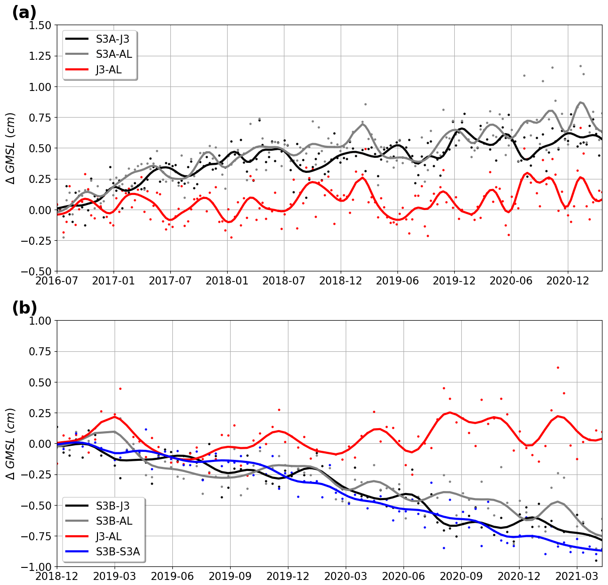
Figure 1 Evolution of ΔGMSL (a) over the S3A period between S3A and Jason-3, S3A and SARAL/AltiKa, and Jason-3 and SARAL/AltiKa and (b) over the S3B period between S3B and S3A, S3B and Jason-3, S3B and SARAL/AltiKa, and Jason-3 and SARAL/AltiKa. The dotted curves are the raw time series sampled at 10 d. The solid lines are time series filtered at 3 months with a low-pass filter. Each time series is artificially set to 0 at its origin.

Other cross-calibration methods could be used in order to estimate the GMSL drift. Among them, the comparison of altimetry and in situ tide gauge (TG) measurements is often used to estimate the GMSL drift estimated from altimetry (Mitchum, 1998; Valladeau et al., 2012; Watson et al., 2015, 2021). Although this method provides very relevant estimates of GMSL drifts for long periods (>10 years), it is not very suitable for shorter and more recent periods. On the one hand, the delay in the availability of the global tide gauge network data (e.g., GLOSS/Clivar) is often more than 1 year and does not allow comparisons with the most recent altimetry data. On the other hand, the uncertainty associated with the calculation of the GMSL drift with this method is large for short periods. It is on the order of 1.5 mm yr⁻¹ over 3 years and 1 mm yr⁻¹ over 5 years (Ablain, 2018; Watson et al., 2021) within a confidence level of 90 % (1.65σ). This method therefore fails to detect a drift of a few tenths of a millimeter per year over the periods of interest in our study. We show in the following sections that the chosen method, i.e., direct altimetry mission comparison, provides more accuracy than the TG altimetry method. However, comparison to tide gauges allows us to obtain an estimate of the GMSL drift with independent measurements. For information purposes, we have therefore provided these values in Sect. 4.

3.2 GMSL drift estimate and uncertainty

In order to estimate the relative GMSL drifts between altimetry missions compared two by two, a rigorous approach is proposed. The first step is to compute the variance–covariance matrix (Σ) of the ΔGMSL time series errors, which is detailed in depth later in this section. The second step consists in fitting the trend from a linear regression model ($y=X\mathit{\beta }+\mathit{ϵ}$) applying an ordinary least-square (OLS) approach, where the estimator of β with the OLS, noted $\widehat{\mathit{\beta }}$, is

$$\begin{array}{}\text{(3)}& \widehat{\mathit{\beta }}\sim {\left(X^{t}X\right)}^{-\mathrm{1}}{X}^{t}y,\end{array}$$

and where the distribution of the estimator $\widehat{\mathit{\beta }}$ takes into account Σ and follows a normal law:

$$\begin{array}{}\text{(4)}& \widehat{\mathit{\beta }}=N(\mathit{\beta },{\left(X^{t}X\right)}^{-\mathrm{1}}\left(X^t\mathrm{\Sigma }X\right){\left(X^{t}X\right)}^{-\mathrm{1}}).\end{array}$$

This mathematical formalism was fully described in Ablain et al. (2019) to estimate the uncertainties of the GMSL trend and acceleration. It is applied in this study to derive the ΔGMSL trend and its realistic uncertainty.

The calculation of Σ is performed from the description of the errors in the GMSL differences between two altimeter missions (ΔGMSL). We have applied the same approach as in Ablain et al. (2019), where the ΔGMSL error budget is composed of different type of errors: (i) drifts in ΔGMSL characterized by a trend uncertainty (±δ) and (ii) time-correlated errors characterized by their standard deviation (σ) and by the correlation timescale (λ). The values of the error budget are deduced from those of the GMSL error budget over the Jason-3 period and are presented in Table 1.

Table 1 Error budget of ΔGMSL between two altimeter missions (ΔGMSL) derived from the GMSL error budget from Ablain et al. (2019).

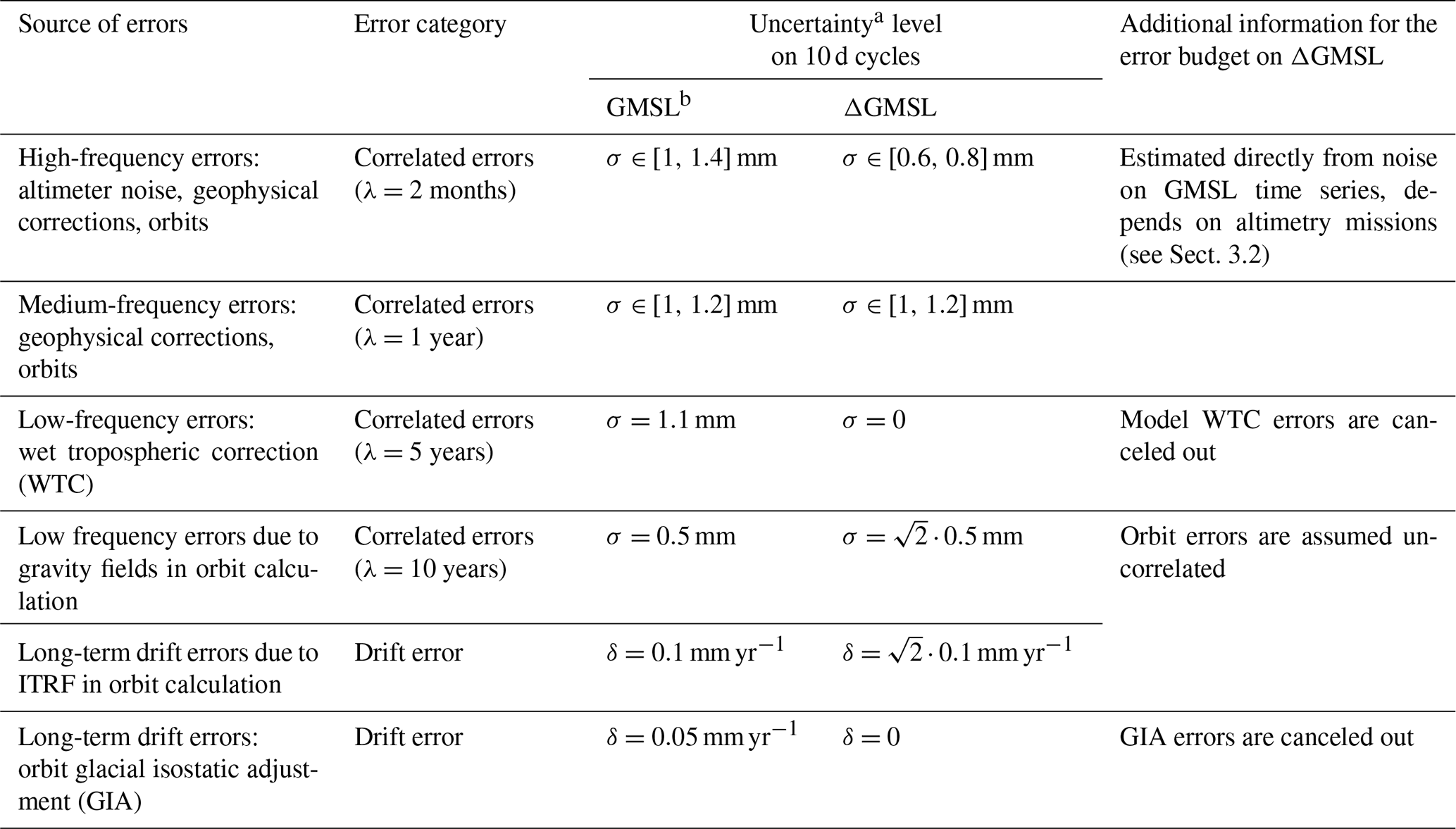
^a All uncertainties reported are based on Gaussian distributions, and they are given at the 1σ level. ^b The GMSL error budget is from the study by Ablain et al. (2019).

Except for altimeter- or radiometer-induced drifts, which are totally independent between missions, or orbit-induced drifts, which can also be totally independent, the drifts that may occur in the GMSL record are atmospheric corrections or tidal corrections that are common to all altimetry missions and are therefore mostly canceled out in the ΔGMSL time series. For instance, the glacial isostatic adjustment correction is derived from the same model (Spada, 2017) for all the missions and does not depend on the altimeter mission characteristics; the error related to the global mean of this correction is then canceled out by comparing GMSL time series. On the other hand, the drift of the realization of the International Terrestrial Reference Frame (ITRF), in which the altimeter orbits are determined provided by Couhert et al. (2015) (δ=0.1 mm yr⁻¹), is assumed to be uncorrelated between two missions that are not on the same orbit (for example S3A and Jason-3). In this case, the uncertainty level of ΔGMSL corresponds to the sum of the variance of the error orbit uncertainty in GMSL ($\mathit{\delta }=\mathrm{0.1}\cdot \sqrt{\mathrm{2}}$ mm yr⁻).

Errors for assessing the drift in the altimeter range by comparing two missions are first due to the errors in altimetry listed by Ablain et al. (2019), which have been identified as having decorrelation timescales of 2 months, 1 year, 5 years, and 10 years depending on the error sources. Secondly, these errors also come from the ocean variability being observed differently by the two missions, which only concerns short timescales (less than 1 year) mainly due to the mesoscale. Therefore, in the GMSL error budget, the residual time-correlated errors can be grouped in two parts: (i) errors with short correlation timescales, i.e., lower than 1 year, (ii) and errors with longer correlation timescales between 5 and 10 years. For the first part, errors in GMSL are mainly due to the geophysical corrections (ocean tides, atmospheric corrections), the altimeter corrections (sea-state bias correction, altimeter ionospheric corrections), and the orbital calculation. As the altimeter sea level is calculated homogeneously for all the altimeter missions in this study (e.g., same ocean tide model, same wet tropospheric correction from model), a significant part of these errors is canceled out in GMSL differences. The remaining uncorrelated errors come from orbital solutions whose errors are independent between altimetry missions at these short timescales. Residual errors in some repeatability-dependent orbit corrections (e.g., aliasing of the ocean tide correction as 58.77 d signal for Jason-3, Zawadzki and Ablain, 2016) may also still be present in the ΔGMSL time series. Another error contribution is coming from the oceanic variability (e.g., mesoscale) being differently observed at short timescales by each altimeter mission due to their different orbit characteristics (Dufau et al., 2016). This error description allows us to consider all high-frequency content of the GMSL time series lower than 1 year as an error signal. The error signal variance is empirically estimated by measuring the variance of the GMSL time series for signals lower than 1 year. Following the approach proposed in Ablain et al. (2019), we split the variance estimate for high-frequency signals (lower than 2 months) and medium-frequency signals (between 2 months and 1 year) in order to better represent the frequency content of the error signal, which is higher at high frequencies, due to the mesoscale signal (<2 months) being observed differently by the altimetry missions. However, the choice of the 2-month cutoff period to separate the high and medium frequencies is somewhat arbitrary. In Sect. 4.2, we have evaluated the sensitivity of varying this period from 1 to 6 months in order to assess the impact on the drift uncertainty estimate, especially over short periods.

For the second part of residual time-correlated errors, between 5 and 10 years, errors in GMSL time series are due, on the one hand, to instabilities in the wet tropospheric correction (Legeais et al., 2018) derived from onboard microwave radiometers, and on the other hand, to the gravity field errors in orbit calculation (Couhert et al., 2015). In ΔGMSL time series; the wet tropospheric correction errors are canceled out since we have applied the same correction for all the altimeter missions derived from the ECMWF model (see Sect. 2). For the gravity field errors in orbit calculation (σ=0.5 mm), they are assumed to be uncorrelated between two altimeter missions that are not on the same orbit (for example S3A and Jason-3). In this case, the uncertainty level ΔGMSL time series is the sum of the variance of the GMSL error budget uncertainty ($\mathit{\sigma }=\mathrm{0.5}\cdot \sqrt{\mathrm{2}}$ mm).

The error variance–covariance matrix (Σ_ΔGMSL) is then inferred from the ΔGMSL error budget for each pair of altimeter missions (e.g., S3A and Jason-3) over the S3A and S3B periods. In short, the elementary variance–covariance matrices (${\mathrm{\Sigma }}_{{\mathrm{Error}}_i}$) corresponding to each error described in the ΔGMSL error budget are first calculated independently of each other. Each matrix is calculated from a large number of random draws (>1000) of simulated error signals whose correlation is modeled. Their shape depends on the type of errors prescribed (e.g., time-correlated errors, long-term drifts). Assuming errors are independent, Σ_ΔGMSL is given by the sum of all ${\mathrm{\Sigma }}_{{\mathrm{Error}}_i}$.

3.3 Extension of the method at regional scales

It is quite straightforward to extend the approach proposed at global scale to derive the ΔGMSL drifts and uncertainties to regional scales. The first step consists of calculating the local mean sea level differences (referred to as ΔMSL hereafter) by averaging the 3^∘ × 1^∘ long/lat SLA grid (see Sect. 3.1) at different spatial scales. For this study, we arbitrarily chose different cell sizes in order to calculate the local MSL drift and its associated uncertainties at different local spatial scales: 3^∘ × 3^∘ (∼ 240 km), 9^∘ × 9^∘ (∼ 700 km), and 30^∘ × 30^∘ (∼ 2400 km). The second step consists of calculating the regional ΔMSL error budget from the regional MSL error budget from Prandi et al. (2021), following the same approach as for the ΔGMSL error budget (Sect. 3.2). The updated values of the ΔMSL error budget are presented in Table 2. In similar fashion to the ΔGMSL error budget, the GIA-induced drift and low-frequency wet tropospheric correction (using model WTC) errors are canceled out. Prandi et al. (2021) evaluate the long-term orbit errors that affect regional MSL at δ=0.33 mm yr⁻¹. Assuming that those errors are independent between two altimeter missions on different orbits, the uncertainty level of the regional MSL time series is the sum of the variance of the regional MSL error budget uncertainty: $\mathit{\delta }=\mathrm{0.33}\cdot \sqrt{\mathrm{2}}$ mm yr⁻¹. For the evaluation of the uncertainty level of short timescale errors, the variance of the error signal is evaluated from the high-frequency content lower than 1 year of regional ΔMSL time series, and the variance estimate is split between a high-frequency signal (lower than 2 months) and a medium-frequency signal (between 2 months and 1 year) to obtain a better frequency representation of the signal. We obtain a location-dependent error signal for high and medium frequencies (see Supplement). The standard deviation of the high-frequency signal below 2 months ranges between 13.3 and 30.7 mm, highlighting the signature of the mesoscale in the large ocean currents. For medium frequencies (between 2 months and 1 year), the variations are weaker: between 6.9 and 17.7 mm. They are also more homogeneous and with a low signature of large ocean currents.

Table 2 Error budget on MSL differences at regional scale between two altimeter missions (ΔMSL) derived from the MSL error budget at regional scale from Prandi et al. (2021).

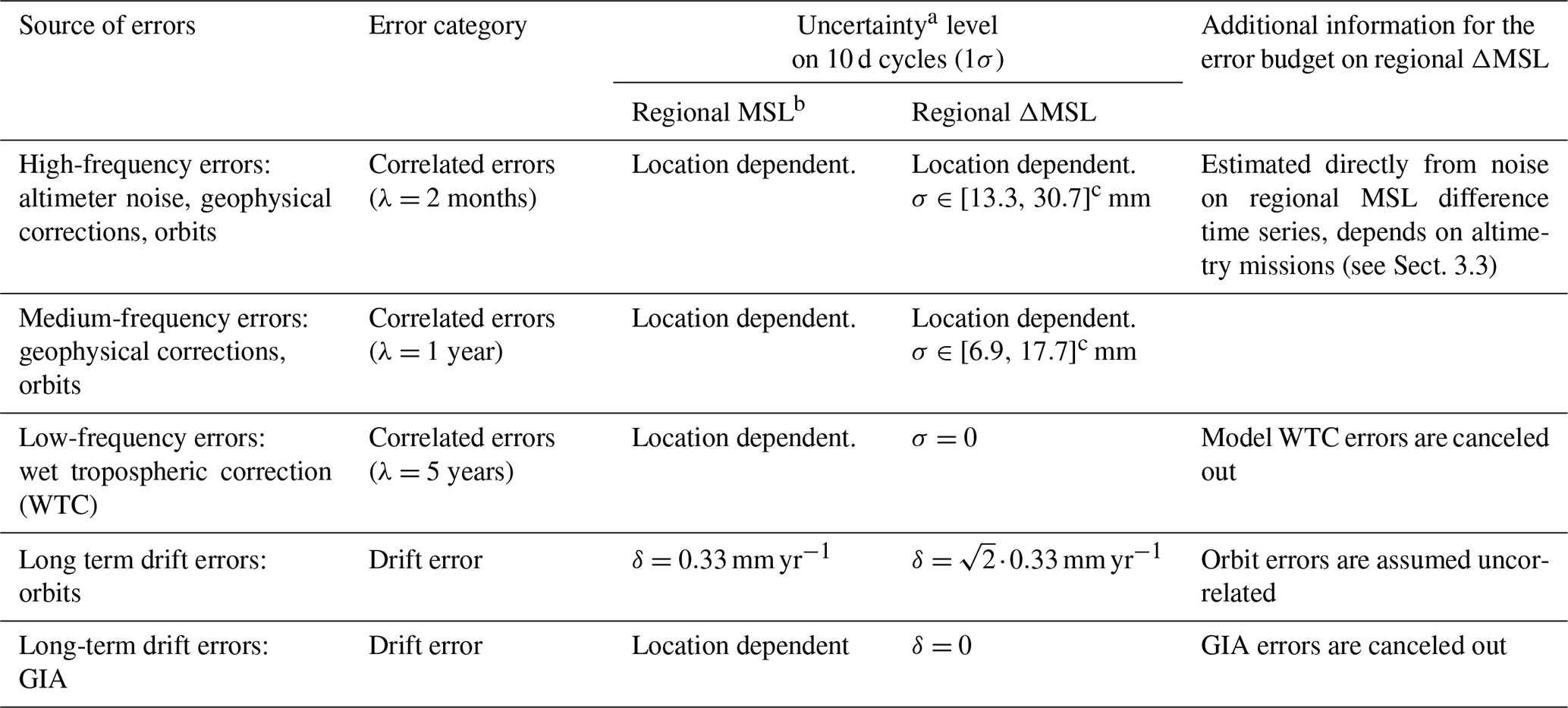
^a All uncertainties reported are based on Gaussian distributions and are given at the 1σ level. ^b The regional MSL error budget is from the study by Prandi et al. (2021). ^c Values provided for 3^∘ × 3^∘ box sizes within a 16th-percentile and 84th-percentile interval.

4 Results

4.1 S3A GMSL drift detection

The ΔGMSL trend and uncertainty is computed using the method provided in Sect. 3.2 between S3A and Jason-3, S3A and SARAL/AltiKa, and Jason-3 and SARAL/AltiKa for a common period between July 2016 and March 2021. Figure 2 shows the ΔGMSL trends and trend uncertainties at 68 % confidence level (CL) (1σ, in black) and 90 % CL (1.65σ in grey) for each of those pairs: 1.01±0.31 mm yr⁻¹ between S3A and Jason-3, 1.28±0.37 mm yr⁻¹ between S3A and SARAL/AltiKa, and 0.29±0.41 mm yr⁻¹ between Jason-3 and SARAL/AltiKa. Calculating the ratio between the ΔGMSL trend and the associated uncertainty, we can indicate the confidence level in which the relative ΔGMSL trend is measured. Between S3A and Jason-3 (as well as between Jason-3 and SARAL/AltiKa), the confidence level at which a trend is detected is 99.9 % (corresponding to 3.4σ). However, a trend between Jason-3 and SARAL/AltiKa is only measured with a low 57.0 % confidence level, and furthermore the estimated ΔGMSL trend value is small (0.29 mm yr⁻¹) compared to the S3A relative ΔGMSL trend with both Jason-3 and SARAL/AltiKa.

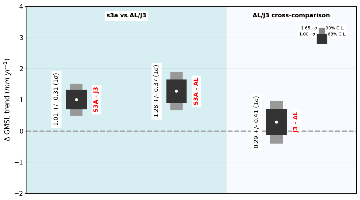
Figure 2 GMSL trend differences between S3A and Jason-3 and between S3A SARAL/AltiKa over the July 2016 to March 2021 period. The black boxes show the GMSL trend uncertainties at 68 % CL, and the grey boxes show the GMSL trend uncertainties at 90 % CL.

These results highlight a significant difference in the GMSL trend between S3A and Jason-3, as well as with SARAL/AtiKa, whereas Jason-3 and SARAL/AltiKa are in agreement within the confidence level. This result likely suggests a drift in the S3A GMSL. Moreover, this result is also confirmed by the comparison with Jason-2, albeit over a shorter period due to the shutdown of Jason-2 in September 2017 (not presented in the paper). The ΔGMSL trend obtained between S3A and Jason-2 is 4.45 ± 0.98 mm yr⁻¹ over the March 2016 to September 2017 period. Over the same period, the ΔGMSL trends obtained between S3A and Jason-3 and S3A and SARAL/AltiKa are 3.66 ± 0.93 and 2.83 ± 1.16 mm yr⁻¹, respectively. Although the trend uncertainties are higher over this shorter period, the ΔGMSLtrends are still significant. These results also indicate that the S3A GMSL drift may have been stronger during its first year of operations. This is confirmed by the analysis of the S3B period (December 2018 to March 2021) in Sect. 4.2, where Fig. 3 exhibits lower ΔGMSL trends of 0.66 ± 0.62 mm yr⁻¹ between S3A and Jason-3 and 1.38 ± 0.90 mm yr⁻¹ between S3A and SARAL/AltiKa.

The very likely drift in the S3A GMSL is also observed through independent comparisons with tide gauges using the method provided by Valladeau et al. (2012) and Ablain (2018) and data from the GLOSS/CLIVAR (GC) tide gauge network. Over the July 2016 to December 2020 period, a significant relative GMSL drift of 1.18 ± 0.63 mm yr⁻¹ (1σ) is also detected between S3A and the GC tide gauge network.

All of these consistent analyses reveal that a drift in the S3A GMSL between 1.0 and 1.3 ± 0.3 mm yr⁻¹ is most likely detected. However, the S3A GMSL drift is much larger than the 0.3 mm yr⁻¹ GMSL PTR-induced drift anticipated by Poisson et al. (2019). Thanks to the results of this study, carried out in the frame of the Sentinel-3 MPC (Mission Performance Centre) project supported by ESA, further studies supported by CNES succeeded in explaining the remaining part of the S3A GMSL drift (about ∼ 0.7–1.0 mm yr⁻¹, Aublanc, 2020). This drift is due to some inner features of the S3 SAR processing that have not been properly considered. A so-called “range walk” correction (not detailed in this paper) was proposed by Aublanc (2020) that will be implemented in the S3 altimeter ground processing chain in early 2022. It is also interesting to note that the 0.3–0.4 mm yr⁻¹ contribution of PTR-induced S3A-GMSL drift is not detectable with a sufficient confidence level over such a short period. One would need a 5-year period to detect a drift of about 0.3 mm yr⁻¹ with a confidence level of about 60 %–70 %.

4.2 S3B GMSL drift detection

In exactly the same fashion as for S3A, the ΔGMSL trends and associated uncertainties are computed between S3B and Jason-3, S3B and SARAL/AltiKa, S3B and S3A, S3A and Jason-3, S3A and SARAL/AltiKa, and Jason-3 and SARAL/AltiKa over a common period between December 2018 and March 2021, i.e., 2 years and 4 months. Figure 3 represents the ΔGMSL trends, and trend uncertainties at 68 % CL (1σ, in black) and 90 % CL (1.65σ, in grey) for each of those pairs.

We can first note that a strong and significant negative ΔGMSL trend is exhibited when S3B is compared to all three other missions: −3.44 ± 0.61 mm yr⁻¹ between S3B and Jason-3, −2.76 ± 0.77 mm yr⁻¹ between S3B and SARAL/AltiKa, and −4.09 ± 0.52 mm yr⁻¹ between S3B and S3A. ΔGMSL trends are significant within a confidence level over 99.9 %. In the meantime, ΔGMSL trends without S3B are much smaller and more consistent over the S3B period: 0.66 ± 0.61 mm yr⁻¹ between S3A and Jason-3, 1.38 ± 0.90 mm yr⁻¹ between S3A and SARAL/AltiKa, and 0.64 ± 0.91 mm yr⁻¹ between Jason-3 and SARAL/AltiKa. Therefore, these results allow us to state that the detection of a drift of the S3B GMSL is very likely with a minimum value of −2.22 mm yr⁻¹ and a maximum value of −4.05 mm yr⁻¹ within a confidence level of 99 %. Furthermore, these results are also confirmed by tide gauge comparisons that indicate a significant drift of the S3B GMSL of −4.04 ± 1.45 mm yr⁻¹ (1σ) over the December 2018 to December 2020 period. At the date this paper was initially submitted, the cause of the S3B drift was unexplained. However, recently Dinardo (2021) found that the drift was due to an inverted sign in the implementation of the of the USO correction. For more information on the USO correction, see the S3 MPC review by Quartly et al. (2020).

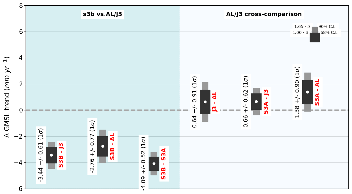
Figure 3 GMSL trend differences between S3B and Jason-3 and between S3A and SARAL/AltiKa over the December 2018 to March 2021 period. The black boxes show the GMSL trend uncertainties at 68 % CL, and the grey boxes show the GMSL trend uncertainties at 90 % CL.

4.3 GMSL trend uncertainty estimates versus the period length

In order to accurately estimate the ability of the proposed method to detect a significant relative drift between two missions, we calculated the evolution of these uncertainties as a function of the period length. In Fig. 4, the solid black line shows the theoretical evolution of the ΔGMSL trend uncertainty between S3A and Jason-3 for period lengths from 1 to 10 years using the error budget presented in Table 1. The ΔGMSL trend uncertainty evolves from 1.75 mm yr⁻¹ for a 1-year period, quickly decreases to 0.5 mm yr⁻¹ for a 3-year period, before slowing down to reach 0.3 mm yr⁻¹ a for 5-year period, and finally converges to 0.2 mm yr⁻¹ for a 10-year period.

We have tested the sensitivity of our uncertainty calculations. Firstly, in Table 1, we have assumed that the GMSL drift caused by the ITRF realization in orbit calculation is uncorrelated between two altimetry missions. It is, however, very likely that this error is strongly correlated even if this information is not quantified in the literature. We have therefore tested the impact of canceling out this error, assuming instead that it is fully correlated between two measurements. The uncertainty level obtained is displayed with the dotted black line in Fig. 4. For a 5-year period, the uncertainty is reduced to 0.27 mm yr⁻¹ (instead of 0.3 mm yr⁻¹), and for a 10-year period it is reduced to 0.13 mm yr⁻¹ (instead of 0.2 mm yr⁻¹). This result has no impact on our study since we have considered the most conservative approach, i.e., the one which yields the highest uncertainties.

Figure 4 Evolution of GMSL trend uncertainties versus period length from the S3A and Jason-3 comparison. The solid black line is the GMSL trend uncertainty derived from the GMSL error budget (Table 1). The dotted black line is the GMSL trend uncertainty derived from the GMSL error budget (Table 1) with the orbit ITRF error contribution set to 0. The red envelope is the dispersion of GMSL trend uncertainty between the 5th percentile and 95th percentile (i.e., 1.65σ) found by varying the cutoff frequency of the high-frequency errors from 0.5 to 6 months.

We have also evaluated the sensitivity of the prescription of high- and medium-frequency errors lower than 1 year. As mentioned in Sect. 3.1, the choice of the 2-month cutoff period is based on the assumption that mesoscale signals are uncorrelated over periods larger than 2 months, but it is somewhat arbitrary. Thus, we have varied the cutoff period for a range of periods from 0.5 to 6 months. The red envelope shown in Fig. 4 represents the dispersion of GMSL trend uncertainty obtained between the 5th percentile and 95th percentile (i.e., 1.65σ). While the variations of the uncertainties can be considered negligible for time periods above 5 years (<0.1 mm yr⁻¹), they are more important for shorter time periods where they reach 0.35 and 0.2 mm yr⁻¹ for time periods of 2 and 3 years, respectively. Given the sensitivity range of our method to estimate uncertainties for periods of 4 years and 9 months (S3A) and 2 years and 4 months (S3B), the drifts observed on Figs. 2 and 3 are still significant. Our conclusions are thus unchanged. However, one should pay attention to it for studies over very short periods of time (<3 years). In addition, it would be relevant to develop other approaches (e.g., based on Fourier analysis) to evaluate the high-frequency spectral content of ΔGMSL time series.

4.4 S3A and S3B regional sea level drift detection

Applying the method described in Sect. 3.3, we evaluated the regional local ΔMSL trends and their uncertainties for S3A and S3B compared to Jason-3 and SARAL/AltiKa for different spatial scales: 3^∘ × 3^∘ cells of ∼ 240 km length, 9^∘ × 9^∘ cells of ∼ 700 km length, and 30^∘ × 30^∘ cells of ∼ 2400 km length. Like for previous sections, the periods considered are 4 years and 9 months for S3A and 2 years and 4 months for S3B. Regional MSL trends are represented in Fig. 5a for S3A and Jason-3 differences on 9^∘ × 9^∘ cells (∼ 240 km regional scale) after removing the global mean trend (i.e., 1.13 mm yr⁻¹). Regional MSL trends range from −2 to +2 mm yr⁻¹, with higher values being found in main large ocean currents (e.g., Kuroshio). In contrast, we do not distinguish between large geographically correlated spatial structures. They might have indicated systematic regional biases in the MSL trends on either of the missions.

The confidence level of the measured regional MSL trends can be obtained by dividing the absolute value of the regional MSL trend by the associated trend uncertainty for each cell. When this ratio is less than 1, the regional MSL trend is less than the uncertainty associated with 1σ and is therefore estimated with a confidence level less than 68 %, i.e., very unlikely. When the ratio is between 1 and 2, the regional MSL trend is estimated with a confidence level between 68 % and 95 %, i.e., likely. When the ratio is greater than 2, the regional trend MSL is estimated with a confidence level greater than 95 %, i.e., very likely. The ratio is represented in Fig. 5b for S3A and Jason-3 differences. We observe that none of the regional MSL trends are significant since they are measured with less than 68 % confidence level. We have performed the same analyses with different sized boxes until 30 × 30^∘ (i.e., 2400 km), and we do not detect any significant regional MSL trend. We also obtain similar results calculating the regional MSL trends between S3B and Jason-3, where we cannot detect any significant trends (see the figures in the Supplement).

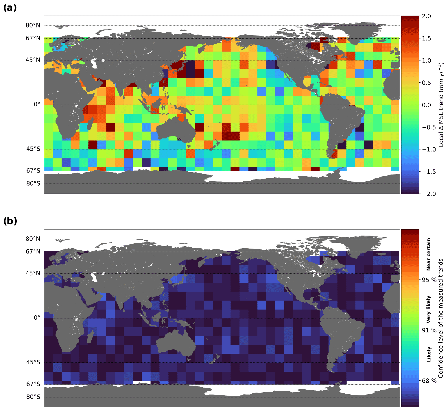
Figure 5 (a) Regional MSL trends between S3A and Jason-3 after removing the global mean trend (i.e., 1.13 mm yr⁻¹ in 9^∘ × 9^∘ resolution). (b) Confidence level of the measured regional MSL trends computed from local MSL trends divided by regional uncertainties between S3A and Jason-3 in 9^∘ × 9^∘ resolution.

The fact that no significant regional MSL trend is detected between S3A and Jason-3 or between S3B and Jason-3 does not demonstrate the absence of regional MSL drift on these altimetry missions. However, this indicates that the level of uncertainty associated with the method implemented is too high to allow the detection of significant trends between these missions. In Fig. 6 we represent the evolution of the regional MSL trend uncertainties versus the period length for the three spatial scales considered based on the S3A and Jason-3 comparison. For a 3-year period, a regional MSL trend over 2.5 mm yr⁻¹ can be detected for the larger 2400 km regional scale (30^∘ × 30^∘) and 5 and 10 mm yr⁻¹ for the 700 km (9^∘ × 9^∘) and 240 km (3^∘ × 3^∘) regional scales, respectively. For a 5-year period, which is a typical period for which two altimetry missions are in orbit simultaneously, a regional MSL trend over 1.5 mm yr⁻¹ can be detected for the larger 2400 km regional scale (30^∘ × 30^∘) and 2.5 and 5 mm yr⁻¹ for the 700 km (9^∘ × 9^∘) and 240 km (3^∘ × 3^∘) regional scales, respectively. These values correspond to a global average but may change locally depending on the high-frequency content of the MSL differences provided in Table 2. The envelopes displayed in Fig. 6 represent the 16th and 84th percentile, corresponding to 1σ of the spatial distribution of MSL trend uncertainties across the oceans. These envelopes show that the uncertainties greatly vary on a local scale (e.g., between 1 and 3 mm yr⁻¹ for a 5-year period and 2400 km box lengths). These spatial variations are mainly due to the mesoscale signal, which is not observed in the same way by altimetry missions (see Supplement). The lowest level of regional uncertainty obtained is 0.75 mm yr⁻¹, with spatial variations between 0.6 and 1.1 mm yr⁻¹, considering boxes of 2400 km over a 10-year period.

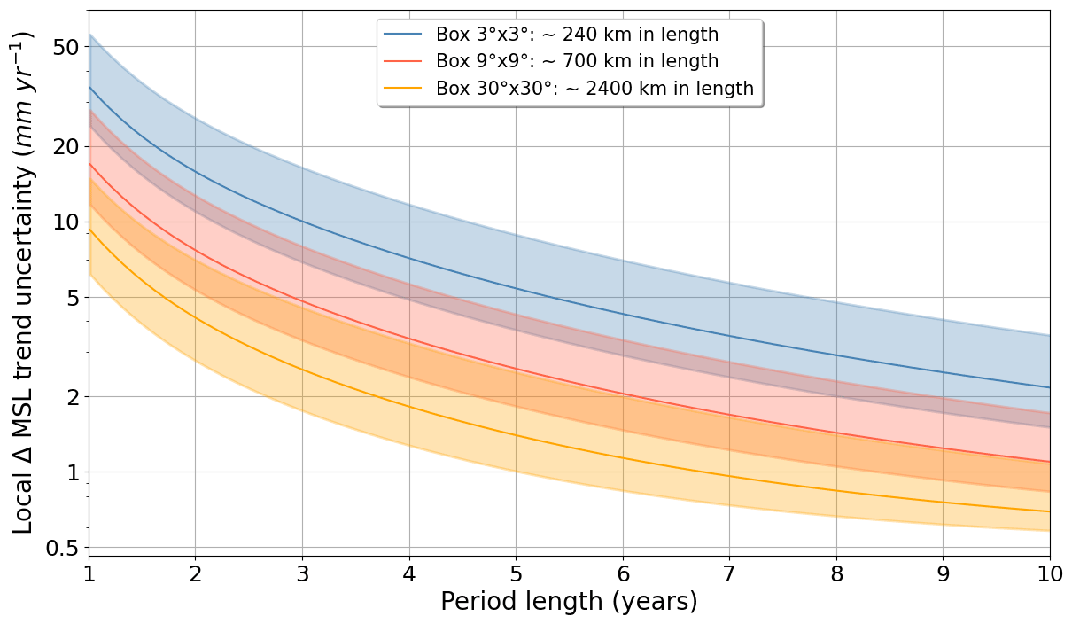
Figure 6 Evolution of the S3A–Jason-3 regional MSL trend uncertainties as a function of period length for different box sizes. The solid line is the global median of regional MSL trend uncertainties. The envelope represents the spatial distribution of uncertainties at between the 16th and 84th percentile (i.e., 1σ) values. The y-axis scale is logarithmic.

5 Conclusions

In this study, we have very likely detected a drift on the Copernicus S3A and S3B GMSL by implementing a method based on cross-comparison to the Jason-3 and SARAL/AltiKa altimetry missions. We have also shown that no spatial variation of the global GMSL drift is detectable for either S3A or S3B within the uncertainty level of the proposed method. For S3A, the detected relative GMSL drift is 1.0 mm yr⁻¹ for Jason-3 and 1.3 mm yr⁻¹ for SARAL/AltiKa, with a more than 99 % confidence level over the July 2016 to March 2021 period. This relative drift is also observed with Jason-2 over a shorter period, as well as when compared to tide gauges. The S3A GMSL drift appears also stronger over the first year of operations: between 2.5 and 4 mm yr⁻¹, with a confidence level higher than 68 %. Thanks to a close cooperation with altimeter experts (in the frame of the S3 MPC project supported by ESA), the origin of the drift is now mainly explained by both a drift on the S3A altimeter PTR parameters, responsible for about 0.3–0.4 mm yr⁻¹ (Poisson et al., 2019), and a drift due to incorrect hypotheses used in the SAR processing (Aublanc, 2020). A correction proposed by Aublanc (2020) (so-called “range walk” correction) will be implemented in the S3 altimeter ground processing chain in early 2022. For S3B, the detected relative GMSL drift is −3.4 mm yr⁻¹ with Jason-3 and −2.8 mm yr⁻¹ with SARAL/AltiKa, with a 99 % confidence level over the December 2018 to March 2021 period. The origin of the drift is an incorrect implementation of the USO correction explained by Dinardo (2021).

By detecting GMSL drifts on S3A and S3B, we have shown the ability of the implemented method to detect relative GMSL drifts for any period length. The typical order of magnitude of relative GMSL drifts that can be detected are as follows: 0.5 mm yr⁻¹ for a 3-year period, 0.3 mm yr⁻¹ for a 5-year period, and 0.2 mm yr⁻¹ for a 10-year period. At the 2400 km regional scale, relative MSL drifts over 2.5 mm yr⁻¹ can be detected over a 3-year period and over 1.5 mm yr⁻¹ for a 5-year period.

Finally, the proposed cross-calibration method allows for the detection of sea level drifts close to the GCOS requirements on sea level stability (Secretariat, G.C.O.S., 2011), which are 0.3 mm yr⁻¹ at the global scale and 1.0 mm yr⁻¹ at regional scales over a minimum 10-year period. Our method is also significantly more accurate than the GMSL drift detected by comparison with tide gauges (Ablain, 2018; Watson et al., 2021): 0.8 mm yr⁻¹ over a 5-year period and 0.5 mm yr⁻¹ over 10-year period. However our proposed approach only detects uncorrelated drifts between missions (e.g., altimeter drift), and not the correlated drifts that might be present in orbit solutions or geophysical correction. Therefore, other approaches based on comparison with independent measurements such as global tide gauges network, are required to estimate sea level drifts of the whole altimeter system. In addition, the comparison between two altimetry missions can be performed over a common period of often less than 8 years, while the comparison between altimeters and tide gauges can be performed over the entire life of an altimetry mission, since the launch of TOPEX/Poseidon in 1992.

Recently, Meyssignac (2019) has identified more stringent sea level stability requirements for climate change studies of 0.1 mm yr⁻¹ at global scale and 0.5 mm yr⁻¹ at regional scales. They cannot be met with our approach, even considering periods of 10 years, or more. We have shown that a better knowledge of the correlation of the orbit error between 2 altimeter missions should be investigated in more detail in future studies. Assuming this error is uncorrelated, we are approaching the GMSL stability requirement of 0.1 mm yr⁻¹ over a 10-year period. Other approaches should also be considered to improve altimeter sea level drift detection. Ablain et al. (2020) proposed to perform two tandem phases between Jason-3 and S6-MF altimeter missions. This particular configuration, where the two satellites follow each other at less than a minute interval, allows for the evaluation of the sea level drifts with an uncertainty of 0.1 mm yr⁻¹ at global scale and 0.4 mm yr⁻¹ at regional scales, over a 3-year period only. However, this new approach, which has not yet been implemented, is applicable only for satellites located on the same orbit. For other satellite configurations, it would also be relevant to analyze cross-comparison methods based on measurement selection at crossovers with a fairly restrictive time difference. This could possibly reduce the effect of oceanic variability in sea level differences and improve the detection of drifts, especially at regional scales.