the Creative Commons Attribution 4.0 License.
the Creative Commons Attribution 4.0 License.
 | 30 Aug 2022
Net community production in the northwestern Mediterranean Sea from glider and buoy measurements
Michael P. Hemming
Jan Kaiser
Jacqueline Boutin
Liliane Merlivat
Karen J. Heywood
Dorothee C. E. Bakker
Gareth A. Lee
Marcos Cobas García
David Antoine
Kiminori Shitashima
The Mediterranean Sea comprises just 0.8 % of the global oceanic surface, yet considering its size, it is regarded as a disproportionately large sink for anthropogenic carbon due to its physical and biogeochemical characteristics. An underwater glider mission was carried out in March–April 2016 close to the BOUSSOLE and DyFAMed time series moorings in the northwestern Mediterranean Sea. The glider deployment served as a test of a prototype ion-sensitive field-effect transistor pH sensor. Dissolved oxygen (O2) concentrations and optical backscatter were also observed by the glider and increased between 19 March and 1 April, along with pH. These changes indicated the start of a phytoplankton spring bloom, following a period of intense mixing. Concurrent measurements of CO2 fugacity and O2 concentrations at the BOUSSOLE mooring buoy showed fluctuations, in qualitative agreement with the pattern of glider measurements. Mean net community production rates (N) were estimated from glider and buoy measurements of dissolved O2 and inorganic carbon (DIC) concentrations, based on their mass budgets. Glider and buoy DIC concentrations were derived from a salinity-based total alkalinity parameterisation, glider pH and buoy CO2 fugacity. The spatial coverage of glider data allowed the calculation of advective O2 and DIC fluxes. Mean N estimates for the euphotic zone between 10 March and 3 April were () for glider O2, (44±94) for glider DIC, (17±37) for buoy O2 and (49±86) for buoy DIC, all indicating net metabolic balance over these 25 d. However, these 25 d were actually split into a period of net DIC increase and O2 decrease between 10 and 19 March and a period of net DIC decrease and O2 increase between 19 March and 3 April. The latter period is interpreted as the onset of the spring bloom. The regression coefficients between O2 and DIC-based N estimates were 0.25 ± 0.08 for the glider data and 0.54 ± 0.06 for the buoy, significantly lower than the canonical metabolic quotient of 1.45±0.15. This study shows the added value of co-locating a profiling glider with moored time series buoys, but also demonstrates the difficulty in estimating N, and the limitations in achievable precision.
- Article
(10149 KB) - Full-text XML
- BibTeX
- EndNote


Around a quarter of anthropogenic carbon dioxide (CO2) emitted between 2011 and 2020 was absorbed by the oceans (Friedlingstein et al., 2022). On timescales of less than a day to many months, CO2 in the ocean is influenced by biological (photosynthesis, respiration) and physical processes (air-sea gas exchange, mixing and advection) (Hood and Merlivat, 2001; Takahashi et al., 2002; Copin-Montégut et al., 2004; Hall et al., 2004; Alkire et al., 2014). Understanding the processes affecting export of carbon from the surface to the interior ocean is key for quantifying the effects of a future warmer climate (Bauer et al., 2013). Whether a location is predominantly autotrophic (dominated by photosynthesis) or heterotrophic (dominated by respiration) determines the sign of net community production, which is defined as gross primary production (by phytoplankton) minus total respiration (by phytoplankton, zooplankton and bacteria) (Alkire et al., 2012).
The surface of the Mediterranean Sea (2.5×10⁶ km2) represents just 0.8 % of oceans globally, but relative to its size, it is regarded as an important sink for anthropogenic carbon dioxide emissions due to higher levels of anthropogenic carbon than in the Atlantic and Pacific oceans (Lee et al., 2011; Schneider et al., 2010). This is due to a low Revelle factor (Broecker et al., 1979) related to relatively warm, salty and high-alkalinity waters, encouraging a net flux of carbon dioxide from the atmosphere to the ocean. Carbon dioxide dissolved in water (CO2(aq) and H2CO3) dissociates to bicarbonate (HCO) and carbonate (CO), releasing H+ ions (Zeebe and Wolf-Gladrow, 2001). CO2(aq), H2CO3, HCO and CO make up total dissolved inorganic carbon (DIC), with HCO accounting for 90 % of DIC. Carbon dioxide absorbed by the ocean is thought to reach the interior via deep water formation and biological processes (Álvarez et al., 2014; Arrigo et al., 2008).
The northwestern Mediterranean Sea displays strong seasonal variability. At the surface, temperatures remain at around 13 to 14 ∘C during winter, increasing to maxima of 26 to 28 ∘C during summer. Wind-driven vertical mixing occurs during autumn and winter, whilst surface stratification is common during summer as a result of solar heating (Copin-Montégut et al., 2004; D’Ortenzio et al., 2008). Vertical mixing can transport nutrients from greater depths to oligotrophic surface waters (Marty and Chiavérini, 2002; de Fommervault et al., 2015). A combination of nutrient availability and increased stability driven by surface warming of 0.2 ∘C can trigger phytoplankton blooms (Yao et al., 2016; Copin-Montégut et al., 2004). The onset of the spring bloom in the northwestern Mediterranean Sea varies from March to April, as observed between 2013 and 2015 at the BOUSSOLE buoy (Bouée pour l'acquisition de Séries Optiques à Long Terme, http://www.obs-vlfr.fr/Boussole/, last access: 20 August 2022) close to the DyFAMed (Dynamique des Flux Atmospheriques en Mediterraneé) site in the Ligurian–Provençal basin (Merlivat et al., 2018). Significant increases in particulate and dissolved organic carbon (POC and DOC) concentrations have been observed during bloom events (e.g. Carlson et al., 1998). POC and DOC export from the ocean surface constitutes the “biological carbon pump” (Carlson et al., 1998; Van Der Loeff et al., 1997; Alkire et al., 2014).
Quantifying these processes in detail requires sufficient data coverage in space and time. Few DIC time series have been maintained continuously, among them the DyFAMed mooring, which is complemented by monthly ship hydrocasts (Copin-Montégut et al., 2004; Antoine et al., 2008; Taillandier et al., 2012). The DyFAMed site is considered an open-ocean location as it is roughly 52 km from the coast in >2000 m deep water. The mooring is useful for studying processes occurring at specific depth levels at one location (Merlivat et al., 2018; Copin-Montégut et al., 2004; Hood and Merlivat, 2001), but a lack of vertical and horizontal spatial information is a limiting factor when quantifying mass and energy budgets. Autonomous underwater gliders have been used to survey the northwestern Mediterranean Sea since 2005 (Niewiadomska et al., 2008; Cyr et al., 2017). They are useful platforms for a range of physical and biogeochemical sensors and can operate autonomously for many months in up to 1000 m deep water using battery power (Eriksen et al., 2001; Piterbarg et al., 2014; Queste et al., 2012). The deployment of autonomous platforms, such as underwater gliders, complements fixed-depth time series by enabling observations of biogeochemical and physical horizontal and vertical gradients. This paper aims to estimate net community production (N) at the DyFAMed site using in situ continuous measurements from a mooring and an underwater glider deployed in March–April 2016. The additional glider data help overcome limitations of the single-depth mooring data in terms of both vertical data coverage and the contribution of horizontal advection. Furthermore, the glider mission served as a test for a prototype ion-sensitive field-effect transistor (ISFET) pH sensor, which complemented the standard temperature, salinity and c(O2) sensors, to provide both O2- and DIC-based net community production.
2.1 Ship measurements
Ship CTD and water sample profiles were collected by RV Téthys II on 7 March and 16 April 2016 at the DyFAMed site (Fig. 1). Ship hydrocast profiles of temperature and salinity (Sea-Bird Scientific SBE 9 CTD), and c(O2) (Sea-Bird Scientific SBE 43 sensor), were supplemented by discrete Niskin bottle samples for c(O2), c(DIC), total alkalinity (AT) and concentrations of total oxidised nitrogen (NO, i.e. the total of NO and NO), silicate (Si(OH)4) and phosphate (PO); see Appendix A for details. Implausible outliers in the CTD profiles (<1 % of values) were flagged and excluded from further analysis.
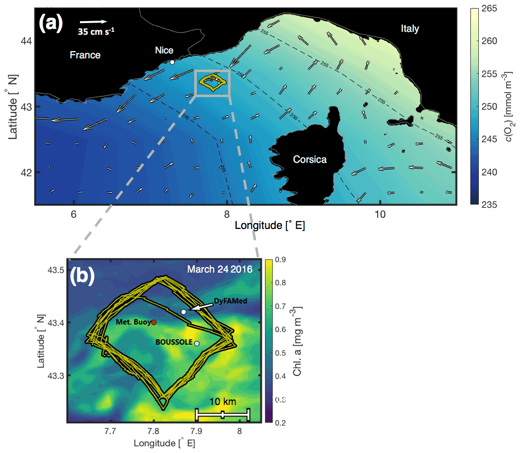
Figure 1(a) The northwestern Mediterranean Sea and glider deployment area (small grey box) superimposed on the World Ocean Atlas 2013 surface c(O2) March climatology (https://www.nodc.noaa.gov/OC5/woa13/woa13data.htm, last access: 20 August 2022), with accompanying AVISO satellite absolute mean surface currents (cm s−1, white arrows) for 6 March–6 April 2016 (http://marine.copernicus.eu/services-portfolio/access-to-products, last access: 20 August 2022). (b) A close-up of the deployment area at the DyFAMed/BOUSSOLE site. The positions of the glider's track (yellow), the DyFAMed mooring (43.36∘ N, 7.90∘ E) (white), the BOUSSOLE buoy (43.42∘ N, 7.87∘ E), and the meteorological buoy “Côte D'Azur” (43.38∘ N, 7.83∘ E) are superimposed on surface chlorophyll a concentrations (https://oceancolor.gsfc.nasa.gov/products, last access: 20 August 2022) on 24 March 2016 (Hu et al., 2012). The bathymetry is flat and greater than 2000 m depth.
2.2 BOUSSOLE and meteorological buoy measurements
At BOUSSOLE, CO2 fugacity f(CO2) (Wanninkhof and Thoning, 1993) at 10 m depth was measured spectrophotometrically via a CARIOCA sensor using the thymol blue pH indicator. Inside an exchanger cell, dissolved CO2 equilibrates with the pH indicator across a silicon membrane. The change in the optical absorbance of the pH indicator is converted to hourly readings of f(CO2) (Hood and Merlivat, 2001), with an accuracy of 3 µatm (Copin-Montégut et al., 2004). The CARIOCA sensor is replaced roughly every 6 months with a newly calibrated instrument (Merlivat et al., 2018). To remove temperature effects, we show f13(CO2), normalised to a temperature of 13 ∘C (Takahashi et al., 1993).
Temperature and salinity were measured hourly using two Sea-Bird Scientific SBE 37-SM MicroCAT sensors at 3 and 10 m depth. The 10 m MicroCAT failed on 15 March 2016. Up to that point, the mean temperature difference between 10 and 3 m was ∘C. The corresponding mean practical salinity S(PSS-78) difference was . The 10 m MicroCAT had the same salinity offset to the ship CTD cast on 7 March. The 3 m MicroCAT agreed to within 0.007 ∘C with temperature and to within 0.006 with salinity of the ship CTD cast on 7 March. A total of 3 d before the ship CTD cast on 16 April, the 3 m MicroCAT also failed. However, its final salinity reading was within 0.01 of the ship value. We therefore used the 3 m MicroCAT temperature and salinity readings for calculating buoy-related results.
c(O2) was measured at BOUSSOLE using Aanderaa oxygen optodes at 3 and 10 m. Only nighttime optode measurements were used because the daytime readings were affected by light-induced spikes (Binetti et al., 2020). Winkler titration samples taken during the ship visits on 7 March and 16 April were used to calibrate optode c(O2) (Coppola et al., 2018).
The meteorological buoy “Côte D'Azur” maintained by Météo-France is located close to the BOUSSOLE buoy (Fig. 1). This meteorological buoy measures wind speed at 3.8 m height above sea level (which is extrapolated to 10 m by adding 10 % of the value), wind direction, air temperature, atmospheric pressure, relative humidity, precipitation and sea surface salinity. Data are archived in the database “SErvice de DOnnées de l'OMP (SEDOO) Mistrals” (http://mistrals.sedoo.fr/Data-Download, last access: 20 August 2022). Wind speed and sea level pressure were used in this study.
2.3 Glider measurements
An iRobot Seaglider model 1KA (sg537; named “Fin”) with an ogive fairing was deployed close to the DyFAMed mooring site. A total of 147 dives (294 profiles) were completed by the glider between 7 March and 5 April 2016, covering a diamond-shaped pattern at 43.22–43.50∘ N, 7.64–8.00∘ E (Fig. 1). The glider completed seven circumnavigations of the survey pattern, each in approximately 4 d, with each of the four sides of the pattern taking approximately 1 d to complete. The glider was equipped with a non-pumped SBE model CTD sensor, an Aanderaa model 4330F oxygen optode sensor, a WET Labs Eco Puck sensor measuring optical backscatter at two wavelengths (470 and 700 nm) and two paired prototype ISFET pH and p(CO2) sensors (Shitashima et al., 2013; Hemming et al., 2017).
Conductivity, temperature and pressure were used to derive potential temperature (θ) and practical salinity (S). Glider c(O2) was calibrated against ship-based c(O2) profiles (Fig. 2a, Appendix B1). Outliers (<1 % of values) outside specified standard deviation ranges (3.5 standard deviations for depths >400 m; 10 standard deviations for depths <400 m) were flagged and discarded from further analysis.
The deployment offered a second opportunity to trial prototype ISFET sensors, previously tested on a glider during the REP14–MED experiment in the Sardinian Sea (Hemming et al., 2017; Onken et al., 2018). ISFET pH was corrected (Fig. 2b) for drift and pressure effects, similar to the steps undertaken by Hemming et al. (2017). The drift- and pressure-corrected ISFET pH was calibrated by linear regression against ship pH on 7 March and 16 April 2016 (Appendix B2).

Figure 2Calibrated glider (a) c(O2) and (b) ISFET pHT over the whole deployment (pale green), 8–9 March (dark green) and 4–5 April (light blue). Ship samples were collected on 7 March (dark green upward-pointing triangles) and on 16 April (light blue downward-pointing triangles).
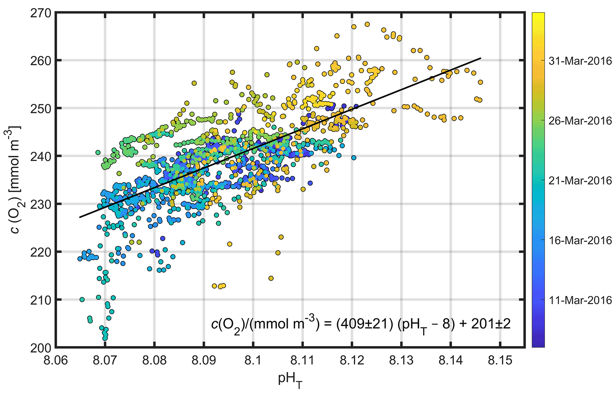
Figure 3Glider pHT against glider c(O2) and coloured by time for all points within the mean euphotic layer (top 46 m). The linear fit and corresponding equation between c(O2) and pHT−8 are also shown.
The spring bloom at the DyFAMed site is characterised by a decrease in surface f13(CO2) due to photosynthesis. Its onset varies from year to year (e.g. April 2013, March 2014) and usually occurs after a period of deep mixing (Merlivat et al., 2018). The glider deployment in March–April 2016 provided horizontal and vertical context to the fixed-depth near-surface mooring sensors when the spring bloom was expected to occur.
Sea surface temperature (SST) remained relatively stable below 13.5 ∘C between 7 and 19 March whilst surface f13(CO2) increased by 40 µatm (Fig. 4a), and surface salinity increased by 0.13 (Fig. 4b). The higher-f13(CO2), higher-salinity waters were likely the results of wind-induced deep mixing and increased convection (Fig. 4a). These waters originate from 50–150 m depth where high-salinity (Fig. 5b), high-f13(CO2), low-c(O2) (Fig. 5c) Levantine Intermediate Water (LIW) exists (Knoll et al., 2017). SST increased by up to 0.6 ∘C between 19 and 20 March and continued to increase intermittently to a maximum of 14.3 ∘C on 5 April (total increase of 1 ∘C over the deployment period).
Whilst SST increased between 19 March and 1 April, f13(CO2) decreased by 85 µatm. This was the start of the spring bloom, associated with increased surface c(O2), pHT and optical backscatter (Figs. 4b, 5c, d, e). O2 is produced by photosynthesis. The pHT increase reflects biological CO2 uptake altering the carbonate equilibria (Cornwall et al., 2013; Copin-Montégut and Bégovic, 2002), and increases in temperature. Optical backscatter relates to predominantly POC (Stramski et al., 2004), with minor contributions from mineral particles and gas bubbles at this site. Therefore, all of these observations suggested an increase in biological production.
A clear relationship between potential temperature (θ), c(O2) and pHT existed within the euphotic layer (mean depth: m) (Figs. 3, 5a, c, e), with higher potential temperature associated with higher pHT and c(O2). The stronger surface stratification resulting from calmer meteorological conditions (e.g. reduced wind speed after 19 March, Fig. 4a) enhanced light supply and stability and caused productivity to increase (Sverdrup, 1953; Pingree et al., 1977). As a result of increased photosynthesis, surface waters became O2-supersaturated by 27 March (Figs. 4b, 5c).

Figure 4(a) Wind speed at 10 m above sea level at the meteorological buoy (dark grey shading), sea surface temperature (pale pink) and CO2 fugacity normalised to 13 ∘C (blue) at 10 m depth at the BOUSSOLE buoy. The partial pressure of atmospheric CO2 in March 2016 (dotted blue) at Lampedusa, Italy, is shown. The onset of the spring bloom (dashed green), determined using buoy f(CO2) measurements, is plotted for comparison. (b) Glider measurements of salinity (orange), optical backscatter at 700 nm (black), dissolved oxygen concentrations (c(O2)) (turquoise) and calibrated pHT (pink) binned at 10 m. The oxygen concentration at saturation (dashed turquoise; parameterisation of García and Gordon (1992) based on Benson and Krause, 1984) is plotted for comparison.
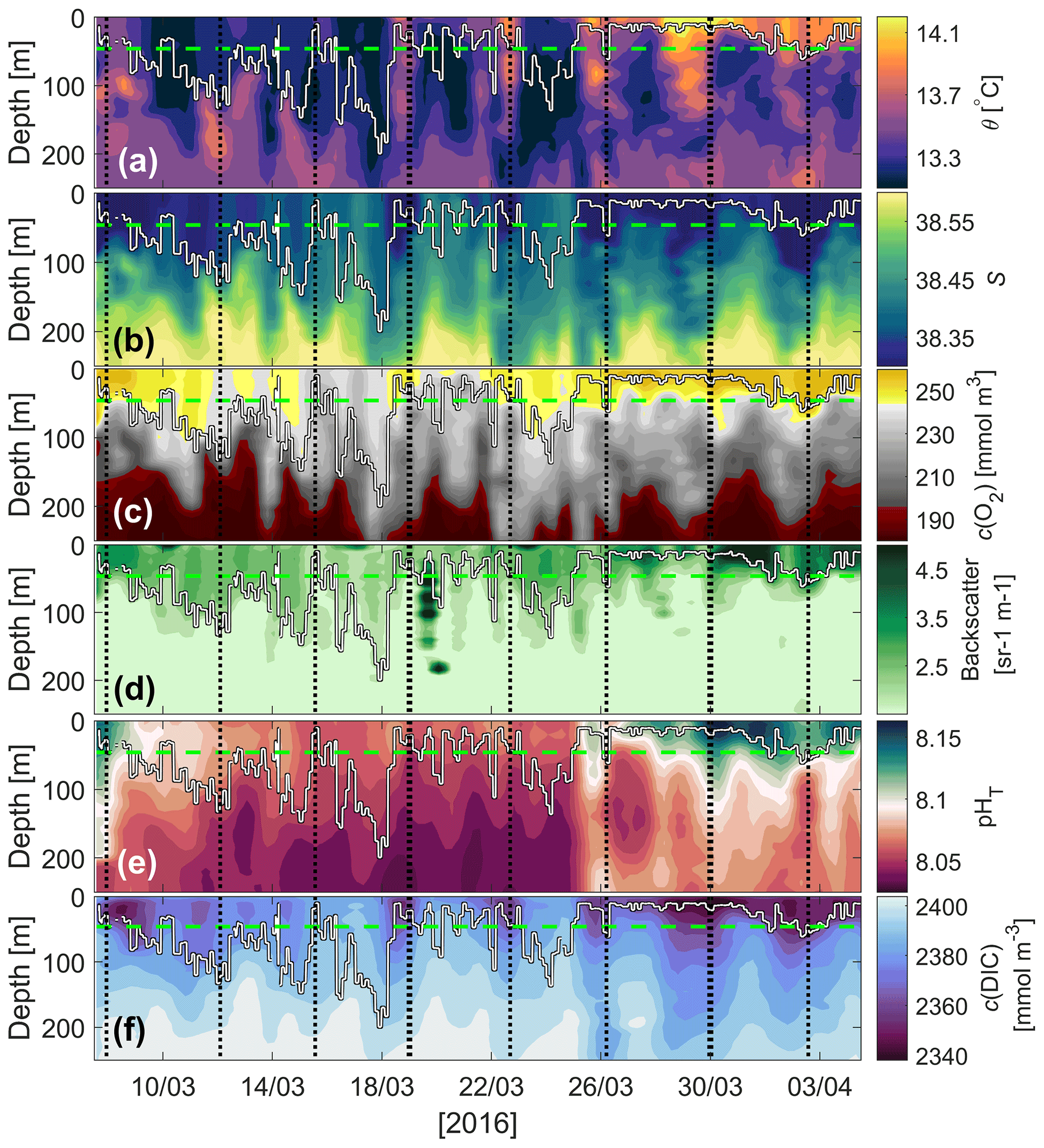
Figure 5Glider (a) potential temperature (θ), (b) salinity, (c) dissolved oxygen concentration (c(O2)), (d) optical backscatter, (e) pHT and (f) dissolved inorganic carbon concentration (c(DIC)). The mean euphotic depth used for calculating N (green dashed line, zlim=46 m) and mixed-layer depth (white line; derived using the potential density criteria of the hybrid scheme of Holte and Talley, 2009) are superimposed. The vertical dashed black lines represent the glider reaching the most northerly point of its transects.
Nutrient concentrations obtained by ship hydrocasts for depths of 10–90 m on 7 March were generally highest at 90 m where there is increased remineralisation and lowest at the surface where there is increased usage by phytoplankton (Fig. 6a). Clear differences can be seen in nutrient samples obtained before and after the spring bloom (Fig. 6b). NO concentrations decreased by 7 mmol m−3, Si(OH)4 by 2.5 mmol m−3 and PO by 0.22 mmol m−3 at 30 m depth, associated with biological production during the spring bloom period. A deep chlorophyll a maximum is often found around this depth (Estrada, 1996) later in the season but was not apparent in our data. At 70 and 90 m depth, nutrient concentrations did not vary much between March and April, while there was a significant decrease in c(O2) and a small change in potential temperature (Fig. 6c). This corresponded to increased stratification with a stronger potential temperature gradient within the top 70 m.
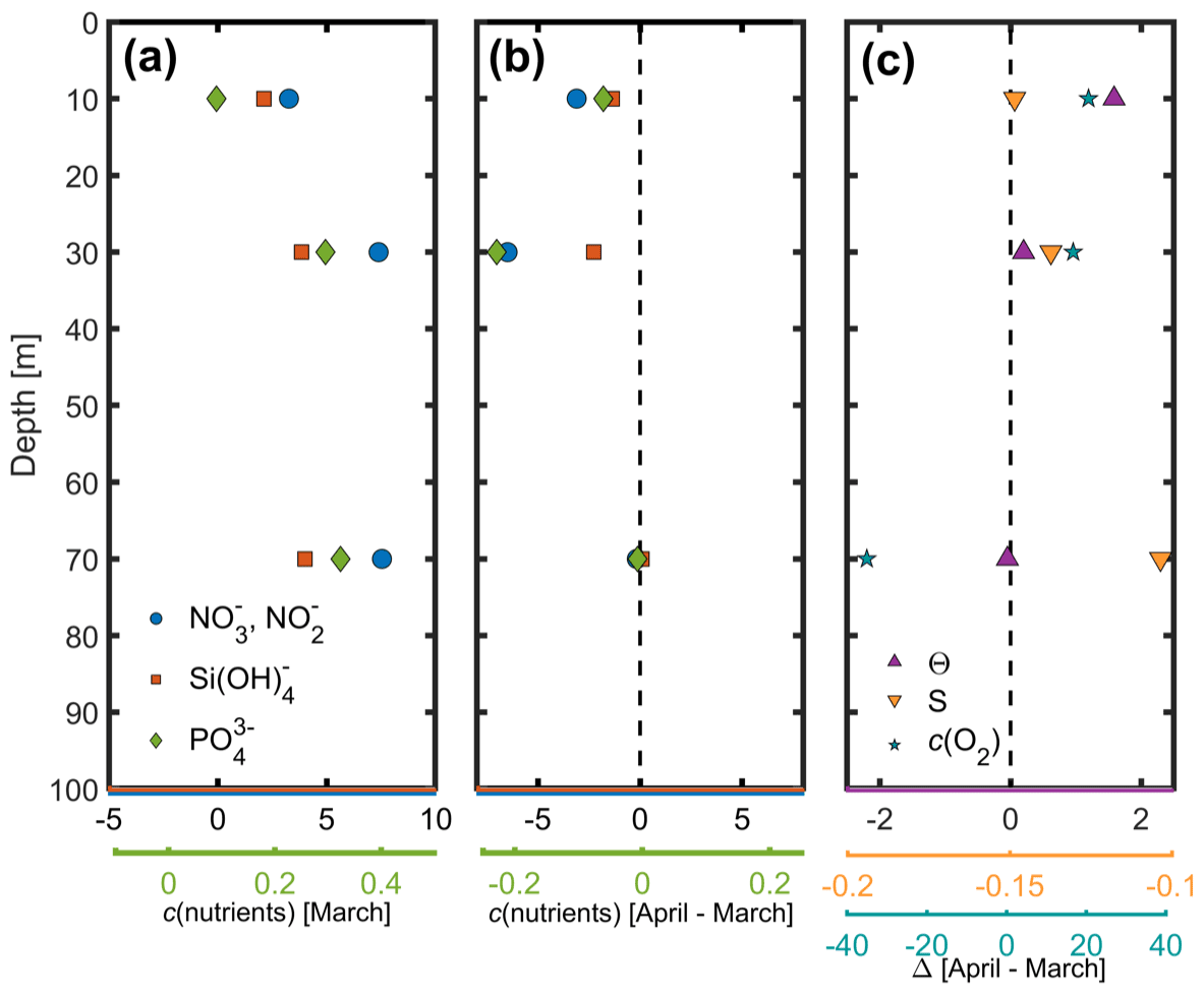
Figure 6(a) Nutrient concentrations (mmol m−3) in March 2016, (b) change in nutrient concentrations between March and April 2016, and (c) changes in potential temperature (θ), practical salinity (S) and c(O2) (mmol m−3) between March and April 2016.
Net community production N is estimated based on mass budgets using the method described by Alkire et al. (2014):
This equation applies to N(O2). For DIC, the N(O2) term is replaced with −N(DIC) because during photosynthesis, DIC is consumed and O2 is produced, and vice versa for respiration.
The following diagnostic equations are therefore used to calculate N based on O2 and DIC mass budgets.
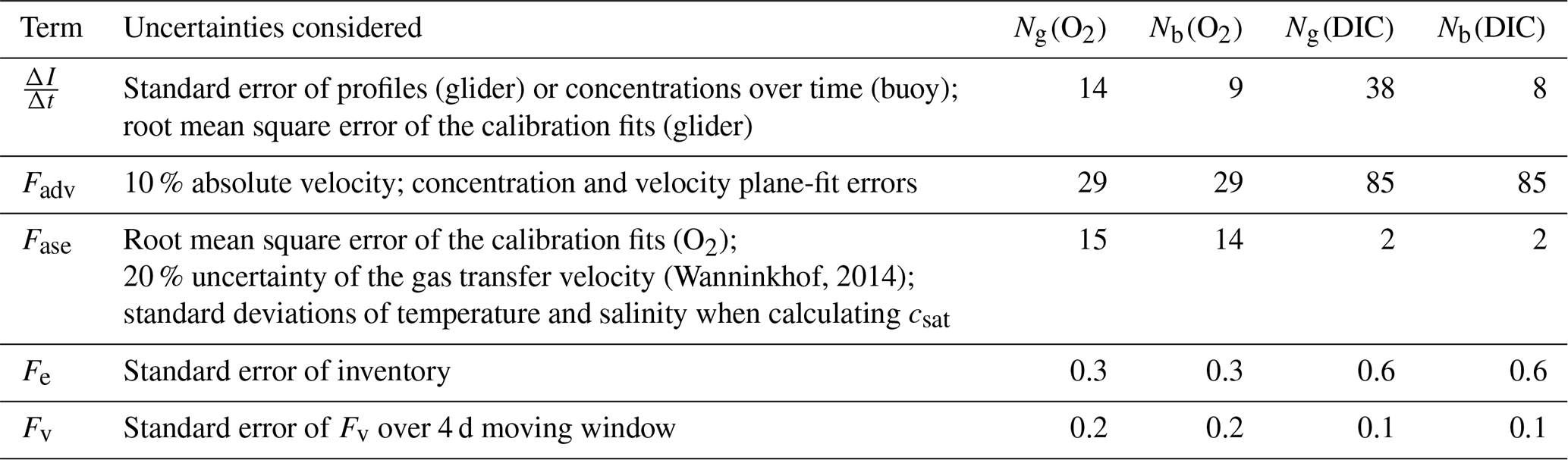
is the integrated column inventory change over time, Fadv is horizontal advection, Fase is the air–sea flux (positive for the direction ocean to atmosphere), Fe is the entrainment flux due to mixed-layer deepening and Fv is the diapycnal eddy diffusion flux. The time period chosen to derive the fluxes required to calculate N spanned 25 d between 10 March and 3 April and included 285 individual profiles (glider dives 10 to 147) spanning the entire survey domain. The first nine dives were omitted because they were used for glider flight trimming. Table 1 gives the uncertainties considered for each budget term. Mean values over the 25 d period are shown in Table 2.
4.1 Inventory change
Daily mean column inventories were integrated between surface and zlim for all glider profiles within a 4 d moving window centred on each date. As integration depth zlim, we used the mean euphotic depth of 46 m, derived from satellite measurements using the method described by Lee et al. (2007). Inventory changes () were calculated from the day-to-day inventory differences.
4.2 Advection Fadv
The glider measured within an Eulerian framework, sampling geographic locations over time. In contrast to a Lagrangian framework, estimates of Fadv are needed to close the budget. Advection was calculated following Alkire et al. (2014) using zonal and meridional mean horizontal concentration gradients and current velocities within zlim using a moving time window of 8 d. This longer time window of 8 d was chosen to reduce the error in the mean gradients (Fig. 7). Mean horizontal concentration gradients Ac(z) and Bc(z) were calculated for each 5 m depth bin using robust plane fits of all concentration measurements in the 8 d time window:
where dc(z) is a constant (not used), and x and y are Cartesian coordinates calculated using zonal and meridional distances, respectively. Bisquare weights were applied when determining the fit coefficients (Gross, 1977) to limit the effect of outliers.
The zonal (east–west) concentration gradients were small for both O2 and DIC (Fig. 8). Opposing meridional (north–south) gradients for O2 and DIC indicate biological patchiness. However, interestingly the positive gradient for O2 (corresponding to higher concentrations in the north) is opposite to the pattern seen in the satellite-derived ocean colour (Fig. 1b), which shows lower chlorophyll a concentrations in the north (implying that the bloom propagates from south to north). This highlights that primary production and net community production are not always directly correlated.
To estimate the absolute geostrophic currents within the survey domain, the dynamic height anomaly (Ψ) was calculated relative to the surface using glider salinity, temperature and pressure (Roquet et al., 2015), and planes were fitted for a moving time window of 8 d:
Using these plane fits, the meridional and zonal components of geostrophic shear were derived and referenced to the 8 d running means of the meridional and zonal components of OSCAR velocities (Bonjean and Lagerloef, 2002). Referencing the geostrophic shear with glider dive-averaged currents (DACs) was initially explored, but when compared with satellite data products (Fig. 8c, d) it was clear that the meridional velocities (v) were unrealistic (see Sect. 7).

Figure 7Plane fits of dissolved oxygen concentrations (c(O2)) at 7.5, 17.5 and 42.5 m depth within zlim for 25 March 2016.
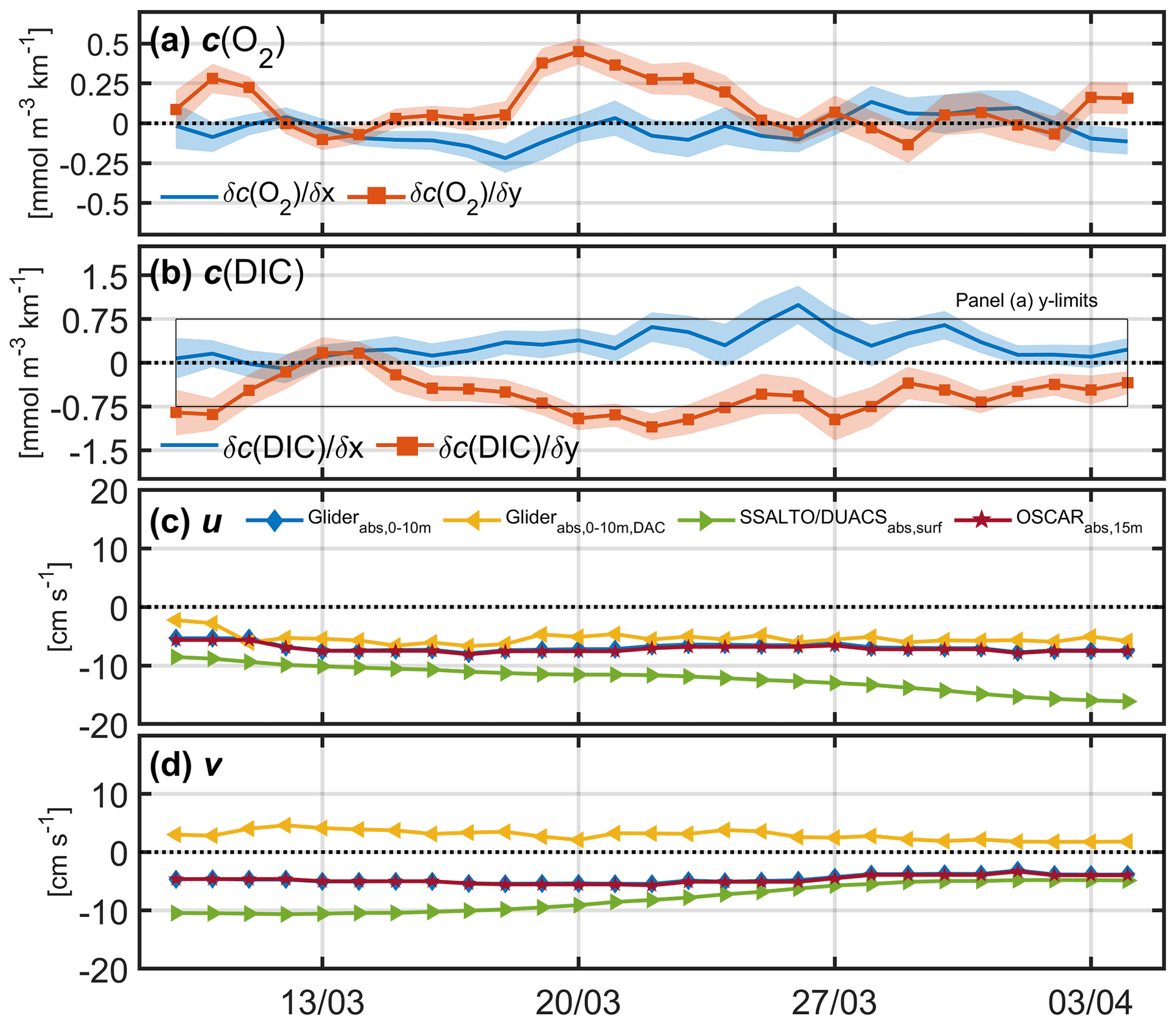
Figure 8Zonal and meridional mean horizontal concentration gradients for (a) c(O2) and (b) c(DIC) estimated using robust plane fits. The black box in panel (b) highlights the y limits for panel (a) for reference. (c) Absolute mean u velocity and (d) v velocity using glider measurements in the top 10 m referenced to OSCAR velocities (blue), and referenced to dive-averaged currents (DACs, yellow), absolute surface mean currents from satellite products SSALTO/DUACS (green) and OSCAR (red).
Table 1The uncertainties considered for each flux term when estimating total propagated error. The mean errors for N using glider (Ng) and buoy (Nb) measurements are listed for both c(O2) and c(DIC) in .
The advection flux (Fadv) was calculated from the horizontal concentration gradients and the absolute geostrophic velocities:
The mean gradients using measurements binned every 5 m between the surface and zlim were averaged at each time step and used for estimating advection (Fig. 8a, b).
4.3 Air–sea gas exchange Fase
Air–sea gas exchange (negative for fluxes from atmosphere to ocean) was estimated for O2 and DIC using
with the equilibrium bubble correction (Woolf and Thorpe, 1991) and
The gas transfer velocity k is calculated according to Wanninkhof (2014). csurf is the mean concentration in the top 10 m over a moving 4 d time window. The mixed-layer depth zmix was estimated using the potential density criteria of the algorithm of Holte and Talley (2009), with a threshold of 0.03 kg m−3 and gradient of 0.0005 . These criteria are sensitive enough to detect the actual mixed-layer depth relevant for gas exchange fluxes (Brainerd and Gregg, 1995). csat(O2) is the O2 air-saturation concentration of García and Gordon (1992), corrected to actual sea-level pressure, pbaro. csat(CO2)=χ(CO2)pbaroF(CO2) is the CO2 air-saturation concentration, calculated using the dry mole fraction of atmospheric CO2, χ(CO2), at the nearest NOAA Carbon Cycle network station Lampedusa, Italy, in March 2016 (ftp://aftp.cmdl.noaa.gov/data/trace_gases/co2/flask/surface, last access: 20 August 2022, site code: LMP, Dlugokencky et al., 2021). F(CO2) is the CO2 solubility function in (Weiss and Price, 1980). The last term of the equations is a scaling factor that apportions the air–sea exchange flux to the depth layer of interest (zlim=46 m) when zmix is deeper than zlim.
4.4 Entrainment Fe
When the mixed layer deepens to depths greater than zlim, water from below with different concentrations mixes with water within the layer. As a result, there is either a reduction or an increase in mean concentration within zlim depending on the vertical concentration distribution. To account for this, Fe was estimated following Binetti et al. (2020):
where I1(zmix(t2)) is the inventory at time t1 within the mixed-layer depth zmix at time t2, I1(zlim) is the inventory at t1 within zlim and t2−t1 represents the time difference. Mean values of zmix and c averaged over a 4 d moving time window were used.
The mean Fe(O2) was () and the mean Fe(DIC) was () for the 7 d in the 25 d period when entrainment (mixed-layer deepening) occurred and zmix>zlim.
4.5 Vertical diapycnal eddy diffusion Fv
Vertical diapycnal eddy diffusion across the base of zlim was estimated using the measured concentration–density gradients (Copin-Montégut, 2000) and an estimate of the turbulence energy dissipation rate ϵ:
where the concentration gradient was evaluated using centred finite differences at zlim±5 m. m2 s−3 was taken from measurements in the Mediterranean bottom pycnoline (Cuypers et al., 2012). Copin-Montégut (2000) guessed a 33 times higher value of m2 s−3 in her study of net community production at DyFAMed, but this value was probably an overestimate because even in the presence of eddies, Cuypers et al. (2012) estimate ϵ to be only m2 s−3. Concentration gradients were calculated for each profile within a 4 d moving window and then averaged to get one gradient per time step.
The mean Fv(O2) was () and the mean Fv(DIC) was () over the 25 d period. With the higher ϵ value of m2 s−3 found in eddies, these fluxes would be 5.7 times higher, but still negligible with respect to the other four terms in the mass budget.
4.6 Buoy measurements
We calculate N from c(O2) and c(DIC) at the BOUSSOLE buoy (Nb) for comparison with Ng estimates. Nb was estimated similarly to Ng, in that we follow the budget approach defined in Sect. 4, and equations defined thereafter. Inventory changes were calculated from surface observations multiplied by zlim because depth profiles are not measured at the buoy. When zmix<zlim, this most likely results in an overestimate of the actual inventory change because N decreases with depth. Also, Fase was scaled in the same way as the glider-based estimates when zmix>zlim. Finally, Fadv, Fe and Fv could not be derived from the single-depth measurements at BOUSSOLE. Instead, the glider-derived fluxes were also used to compute Nb.
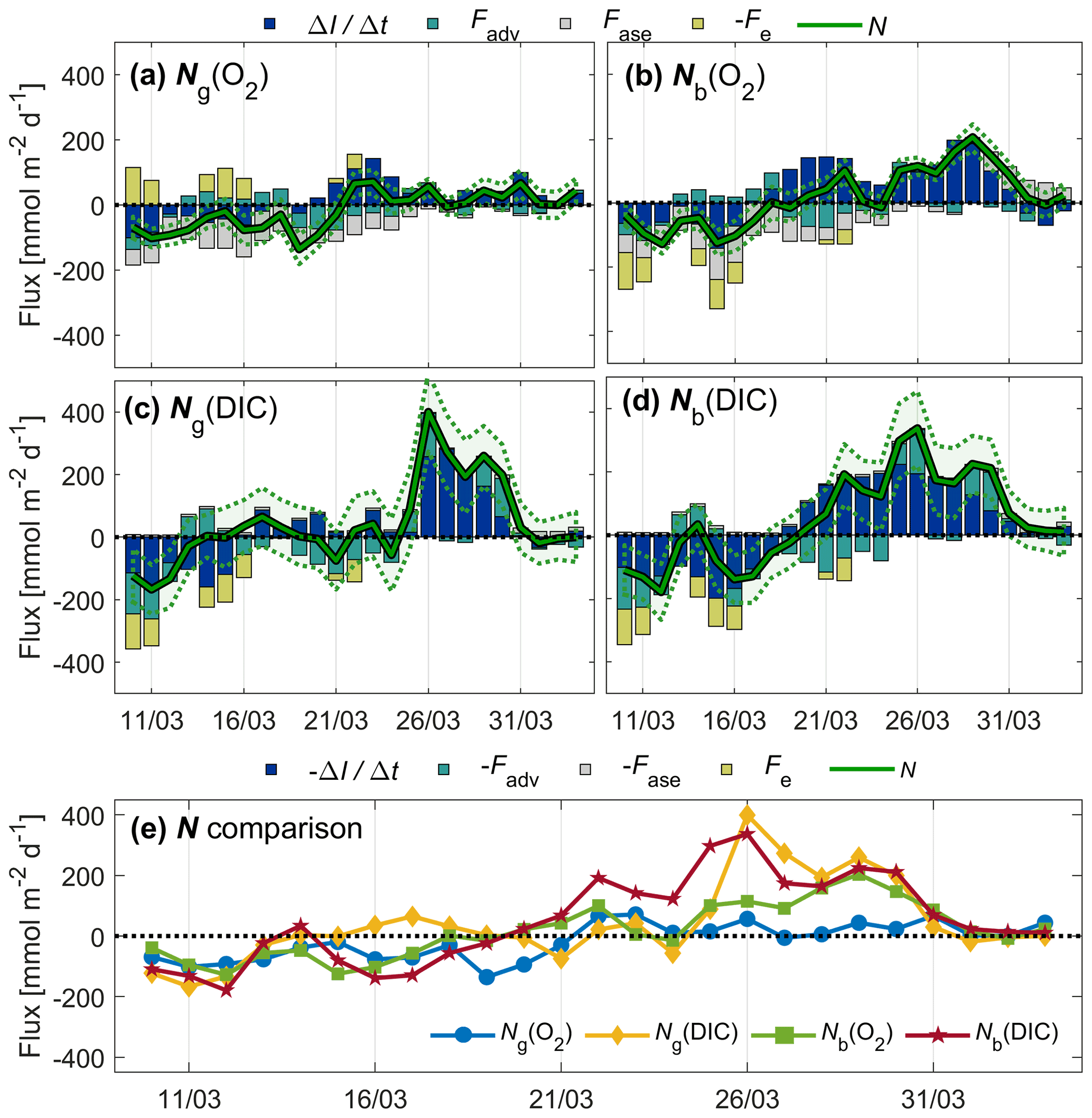
Figure 9Inventory change (), advection (Fadv), air–sea exchange (Fase), entrainment (Fe) fluxes, and net community production (N) of O2 (a, b; top legend) and DIC (c, d; bottom legend) related to glider (a, c) and buoy (b, d) measurements. Uncertainty intervals are shown as dotted lines. All N estimates are compared in panel (e).
Prior to 21 March, Ng and Nb were negative or close to zero most of the time (Fig. 9e). This could be a sign of local net heterotrophic conditions, but could also be due to underestimated entrainment (Fe) or vertical eddy diffusion fluxes (Fv). This observation cannot be explained by physical undersaturation driven by recent cooling because temperatures decreased by only 0.2 ∘C between 1 and 21 March, explaining at most 0.4 % undersaturation. After 21 March, N exceeds zero until the end of the deployment period. The approximate start of the spring bloom was 19 March as evidenced by the buoy c(DIC) (Fig. 4), which is also the time when Nb(DIC) becomes positive, lasting until the end of the deployment period.
Coppola et al. (2018)Copin-Montégut (2000)Table 2Comparison of , Fadv, Fase, Fv and N estimates using c(O2) and c(DIC) and the corresponding flux terms used in this study with others in the literature. The N estimates of Copin-Montégut (2000) are based on , Fase and Fv (calculated with a turbulence energy dissipation rate of ).
Ng(O2) peaks on 22–23 and 31 March at around 70 , matching periods of high c(O2) (Fig. 5c). In contrast, Nb(O2) is highest between 25 and 31 March at ≥80 . The total range of N(DIC) is larger than for N(O2). Ng(DIC) and Nb(DIC) reach similar peak values on 26 and 29–30 March.
The contributions of Fadv and Fe are significant at times. on days when wind is high and the surface mixed layer is deepening (Fig. 9), and there are periods when absolute Fadv(O2)>50 . Absolute Fadv(DIC) is on average 34 higher than Fadv(O2), and on some days absolute Fadv(DIC)>100 . Fe(DIC) is generally of similar magnitude to absolute Fe(O2). Surface waters are undersaturated with O2 prior to 29 March (negative Fase) and then oversaturated until the end of the deployment period (positive Fase). Surface waters are undersaturated in CO2 throughout the deployment period (negative Fase).
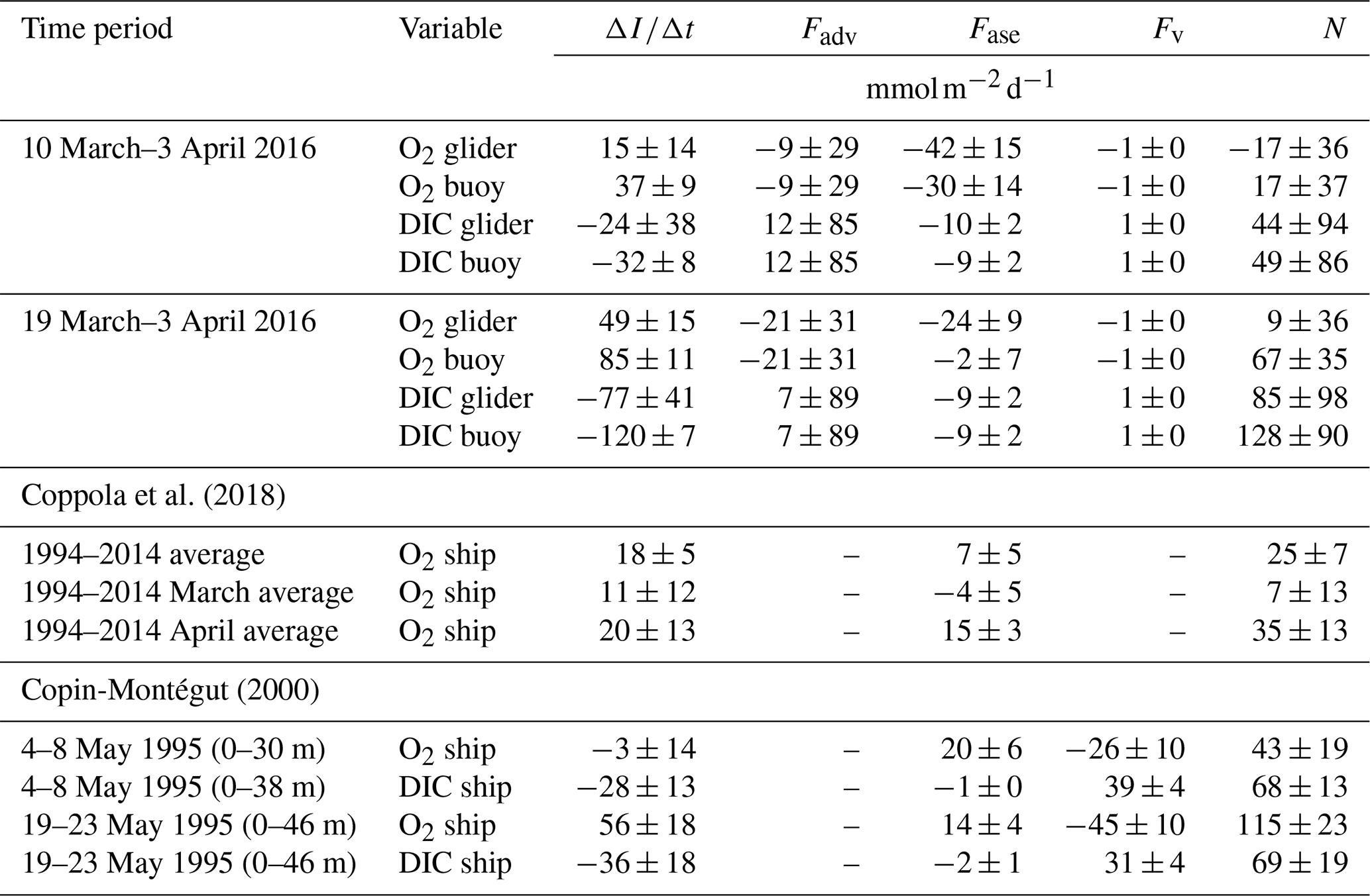
Between 10 March and 3 April we estimate an average N of between () and (49±86) , depending on the variable used (Table 2). Between 19 March and 3 April, N was positive most of the time and on average ranged between (9±36) and (128±90) .
Dividing N(O2) by N(DIC) provides the photosynthetic quotient QP, previously estimated as 1.45±0.15 (Laws, 1991; Anderson and Sarmiento, 1995; Anderson, 1995). The average QP in this study using Ng(O2) and Ng(DIC) between 10 March and 3 April was 0.14±0.81, excluding periods when Ng(DIC)<30 (i.e. close to zero within its uncertainty). When using Nb(O2) and Nb(DIC) over the same time period, average QP was 0.49±0.60. Using linear regression of N(O2) against N(DIC) provides another way to derive QP. The resulting slopes are 0.25±0.06 for the glider and 0.54±0.06 for the buoy N estimates. These QP values therefore do not match the canonical values of 1.45±0.15, but similarly low values of 0.63±0.30 were observed by Copin-Montégut (2000) in early May 1995 at the same site (Table 2).
The change of nutrient concentrations provides an alternative to estimating net community production. Assuming the observed NO drawdown of 7 mmol m−3 and the PO drawdown of 0.22 mmol m−3 occurred over a period of 15 to 25 d (with 15 d corresponding to the period 19 March to 3 April; the exact period is not known because we only have observations on 7 March and 16 April) and extends over the same depth horizon (46 m) as used for the O2- and DIC-based N calculations, and neglecting any additional contribution to net community production fuelled by diapycnal mixing, this corresponds to rates of 13 to 21 mmol for nitrogen and 0.4 to 0.7 mmol for phosphorus. Assuming a Redfield stoichiometric ratio of (Redfield et al., 1963), this corresponds to carbon fluxes of 85 to 142 (based on nitrogen) and 43 to 72 (based on phosphorus). The values are in reasonable agreement with the N(DIC) values derived for the bloom period between 19 March and 3 April of (85±98) to (128±90) , indicating nutrient consumption in line with the assumed stoichiometric ratio.
The discrepancy between Redfield and observed stoichiometry is larger for the O2-based net community production, especially for the glider-based values. Non-Redfield ratios have been documented before, including at the same site. For example, Copin-Montégut (2000) found non-Redfield ratios for O2 and DIC-derived N at DyFAMed. Hull et al. (2021) found non-Redfield ratios for O2- and nitrate-derived N in the North Sea. We do not have a physiological explanation for such large deviations from the canonical stoichiometric values. It is unlikely to be due to a calibration error in the O2 concentration because it would have to be of the order of 20 mmol m−3, and our observations at depths >400 m agree to within 3 mmol m−3 with the record of historic measurements.
Quantifying net community production helps us to understand the role of biological production and consumption on carbon export from the surface to deep waters. If the rate of carbon export is known, the rate of atmospheric CO2 drawdown into the ocean can be better quantified, and the accuracy of future climate projections might improve. Using underwater gliders as tools to observe the water column on timescales of less than a month over a wider area allows us to estimate physical processes (e.g. mixing, advection) that affect biogeochemical tracer concentrations and estimates of net community production derived therefrom.
During the spring bloom (19 March to 3 April) we estimate N between (9±36) and (128±90) on average, with maxima >300 at times. Few studies have estimated N at the DyFAMed site, and there are currently no N estimates that incorporate Fadv using concentrations over a larger area surrounding DyFAMed.
Another study at this site estimated an annual mean N(O2) of (25±7) (equivalent to 9.2 ) and monthly mean O2 production of (7±13) and (35±13) in March and April, respectively, using excess O2 above 100 % saturation over a period of 20 years (Coppola et al., 2018). Furthermore, Copin-Montégut (2000) estimated N(O2) as (43±19) in the top 30 m from 4–8 May 1995 and as (115±23) in the top 46 m from 19–23 May 1995. A direct comparison is not possible between this study, Coppola et al. (2018) and Copin-Montégut (2000) because each study is based on different timescales (from years to days), different vertical integration horizons and different seasons. Keeping this in mind, our range of N estimates is similar to those of Coppola et al. (2018) and Copin-Montégut (2000).
We can compare our study with other studies elsewhere that estimate N using glider measurements. Alkire et al. (2014) estimated mean N(O2) as (65±25) over a 23 d period in June 2008 in the North Atlantic. Like our study, they estimated N(O2) incorporating Fadv derived using horizontal gradients measured by a glider. Further, Hull et al. (2021) estimated N(O2) as (154±2) in the North Sea in April 2019.
Uncertainties for N(DIC) are generally higher than those for N(O2), and the highest uncertainties are associated with Fadv. Fadv uncertainties are high because the uncertainties associated with the concentration plane fits are high due to c(DIC) variability within the time-centred window. For example, c(DIC) within zlim varied over 33 mmol m−3 for the time-centred window on 16 March, leading to low standard errors (Fig. 8b), while c(DIC) varied over 40 mmol m−3 for the time-centred window on 26 March, leading to high standard errors. For this latter window centred on 26 March, the decrease in c(DIC) over time between 25 and 30 March caused this high uncertainty. We use an 8 d time-centred moving window to reduce the potential effect of biologically related concentrations on the mean gradients, typically seen on short timescales. However, as demonstrated here, a trade-off is the higher uncertainty. Additional gliders deployed in future missions could potentially decrease the uncertainty associated with Fadv by combination of alternative sampling strategies, leading to more measurements in horizontal space and thus improving the robustness of the plane fits.
We initially explored using the glider DACs to reference geostrophic shear, required to estimate Fadv. However, DAC v velocities were positive throughout most of the deployment period in an area where negative v velocity is expected, as seen in satellite data products (Fig. 8). We think the erroneous DAC v velocities relate to the glider's roll during flight, which was consistently starboard. The disadvantage of using OSCAR velocities to derive velocity profiles relates to resolution; OSCAR velocities are derived every 8 d on a grid with 0.25∘ resolution.
The Nb estimates incorporate measurements at a depth of approximately 10 m that we extrapolate over the average euphotic depth (zlim=46 m), while Ng estimates account for the vertical variability between the surface and zlim. This means that the glider-based N estimates should in principle be more accurate. It also explains why the buoy-based inventory changes are larger than for the glider, due to concentrations varying more near the surface than at depth.
We chose zlim=46 m as the integration depth for estimating N. We investigated the sensitivity of the integration depth to N estimates by estimating N over the top 36 m and top 56 m of the water column. We found that N estimates are not very sensitive to the integration depth; e.g. using zlim=36 m, we obtain N values between (11±28) and (113±75) for the period 19 March to 3 April. Using zlim=56 m, we obtain N values between (3±44) and (147±109) .
The spring bloom started in this area of the northwestern Mediterranean Sea around 19 March 2016. We identified the spring bloom through a decrease in the DIC concentration (inferred from a pH increase) and an increase in the oxygen concentration. The spring bloom followed a period of high winds and a well-mixed higher nutrient water column. The glider also detected increased optical backscatter with spikes on 19 and 20 March, an indication of increased particle concentrations. The spring bloom start date fell into the time frame of phytoplankton blooms in previous years according to buoy-based sensors. However, this was the first time that high-resolution glider profiles were available, providing insights into the biogeochemical and physical processes at depth and in waters horizontally surrounding the DyFAMed mooring.
This study demonstrates the potential of using autonomous glider measurements for estimating net community production (N). It is the first study of this kind in the northwestern Mediterranean Sea. Both oxygen and dissolved inorganic carbon concentrations were used to derive mass budgets, taking into account N, air–sea gas exchange, horizontal advection, vertical entrainment and diapycnal eddy diffusion. Estimating N using different data sets was challenging, which is reflected in the range of N estimates and their uncertainties presented here. We found that day-to-day variations in derived N estimates were dominated by net inventory changes, air–sea exchange and horizontal advection. Entrainment only came into play on 7 out of 25 d, i.e. during periods when the mixed-layer depth deepened beyond the integration limit of the mean euphotic zone depth of 46 m. Diapycnal eddy diffusion was negligible at all times. Over the duration of the deployment from 10 March to 3 April, we estimate N over the mean euphotic zone depth to be () based on glider O2, (44±94) based on glider DIC, () based on buoy O2 and (49±86) based on buoy DIC. Within their uncertainties these values agree and show net metabolic balance. Unlike previous studies in this region of the northwestern Mediterranean Sea, our results and their uncertainties explicitly consider the role of horizontal advection.
We showed that advection can potentially be significant in the area of our study, bearing in mind that the associated uncertainty was high. Daily mean N values estimated from point measurements typical of fixed moorings were affected by advection on some days. Advection may also be relevant on timescales longer than 1 month, but the current study was too short to explore this. However, when the advection flux was averaged over the 25 d period, there was less of an effect on N, suggesting that at least in this region, its importance might diminish for longer integration periods. To better resolve the influence of advection on shorter timescales and reduce its uncertainty, similar future studies should increase the number of gliders circumnavigating the central mooring so that averaging intervals can be reduced and the time resolution can be enhanced.
This was the second test deployment of the prototype ISFET sensors on gliders, following our first test in 2014 (Hemming et al., 2017). There were still considerable problems with drift and a need for calibration. Since then, Saba et al. (2018) and Takeshita et al. (2021) had more success with a Sea-Bird Scientific ISFET sensor and a Deep-Sea-DuraFET sensor, respectively. However, these sensors are not yet commercially available for gliders.
Water samples used to measure c(O2) were collected at the DyFAMed site on 7 March (n=10) and 16 April 2016 (n=8) using 12 L Niskin bottles (General Oceanics 1010X) from the top 1000 m of the water column; four samples each were from the top 100 m (Fig. B1b). Reagents needed for the fixation of oxygen were added to the samples at the time of water sample collection on board the ship. An automated Winkler titration method with endpoint detection was used after each cruise in the laboratory at the Observatoire Océanologique de Villefranche-sur-Mer, France, to determine c(O2). Replicates were obtained to determine precision. c(O2) measured by the rosette-mounted SBE43 sensor within the top 150 m was 15 mmol m−3 higher than the Winkler measurements (Fig. B1b). SBE 43 sensor c(O2) was corrected by regressing against the Winkler c(O2) values. The resulting regression coefficients were 0.892 ± 0.009 for slope and for intercept on 7 March (r2=0.9993; σ=0.9 mmol m−3). The corresponding values on 16 April were 0.920 ± 0.008 and (r2=0.9997; σ=0.7 mmol m−3).
A Marianda Versatile INstrument for the Determination of Titration Alkalinity (VINDTA 3C; https://www.marianda.com, last access: 20 August 2022) was used to measure c(DIC) and AT at 10 depth levels. A total of 19 bottles of certified reference material (CRM) supplied by Scripps Institution of Oceanography (San Diego, California, USA) were run to calibrate the instrument. Coulometry following standard operating procedure SOP 2 was used to measure c(DIC) (Dickson et al., 2007; Johnson et al., 1985), and potentiometric titration following SOP 3b was used to measure AT (Dickson et al., 2007).
Nutrients at DyFAMed were measured using water collected in the same Niskin bottles as those used for c(O2), c(DIC) and AT. Samples were analysed via a standard automated colorimetry system (Seal Analytical continuous flow AutoAnalyser III) at Observatoire Océanologique de Villefranche-sur-Mer for NO (nitrate NO and nitrite NO combined) (Bendschneider and Robinson, 1952), Si(OH)4 (Murphy and Riley, 1962) and PO (Strickland and Parsons, 1972), with detection limits of 0.01, 0.02 and 0.02 mmol m−3, respectively (de Fommervault et al., 2015).
B1 O2 measurements
Glider c(O2) values were calibrated to take into account the response time (τ) of the sensor, which is dependent on the thickness, and usage of the sensor foil (McNeil and D'Asaro, 2014), as well as temperature, and to account for the difference between the glider measurements and c(O2) obtained by the ship (Fig. B1b) (Binetti et al., 2020; Hemming et al., 2017). To correct c(O2) measured by the glider sensor, the sensor-related oxygen engineering parameters TCPhase and CalPhase were used. A mean τ of 8 s was applied to correct measurements for the sensor time lag. This mean τ value was determined from the lowest root mean square difference between descending and ascending TCPhase profiles shifted in time by values of τ ranging from 0 to 50 s. After lag correction of the glider TCPhase, the relationship between the ship sensor pseudo-CalPhase measured on 7 March and on 16 April and the glider TCPhase measured on 8 March and on 4 April was determined (Fig. B1a). The ship sensor pseudo-CalPhase was calculated from the calibrated ship sensor c(O2) by inverting the set of equations normally used to obtain c(O2) from glider optode TCPhase and CalPhase. The slope and offset coefficients obtained from the relationship between the glider TCPhase over the entire deployment time period and ship sensor pseudo-CalPhase on 7 March and 16 April (Fig. B1a) were linearly interpolated over the duration of the deployment. The interpolated coefficients were matched with glider measurements in time and used to correct all glider CalPhase profiles obtained during the deployment, allowing a calibration of glider c(O2) (Fig. B1b). After calibration, the glider c(O2) agreed with buoy c(O2) (Fig. B1c), as would be expected because the same Winkler samples were used to calibrate ship and buoy oxygen sensors.
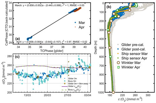
Figure B1Calibration of the glider dissolved oxygen concentration (c(O2)) sensor. (a) The linear regression fit using back-calculated ship pseudo-CalPhase and glider TCPhase for 7 March (blue) and 16 April (orange), along with the corresponding linear equations, r2 and root-mean-squared errors (RMSE). The 95 % confidence bounds are also shown. (b) Glider c(O2) measured on 8–9 March and on 3–4 April before (grey), and after (blue) calibration, the ship sensor c(O2) on 7 March (yellow) and on 16 April (green), and the c(O2) Winkler samples on 7 March (white with orange border) and on 16 April (white with green border). (c) All glider sensor c(O2) at 3 m depth (blue stars), <5 km away from the BOUSSOLE buoy only (turquoise spots) and glider csat (purple line) are compared with the BOUSSOLE buoy sensor c(O2) measurements (orange spots) at 3 m depth and buoy csat (green dashed line).
B2 ISFET pH measurements
The deployment offered a second opportunity to trial two prototype ISFET pH–p(CO2) sensor pairs, previously tested on an underwater glider in the Sardinian Sea during the REP14–MED experiment (Hemming et al., 2017; Onken et al., 2018). The sensors are custom-built non-commercially by Kiminori Shitashima's group at Tokyo University of Marine Science and Technology, Japan. ISFET sensors measure pH using the interface potential between a reference chlorine electrode (Cl-ISE) and a semiconducting ion sensing transistor (Hemming et al., 2017).
One pH–p(CO2) sensor pair was stand-alone, meaning measurements were logged and stored by the sensor and retrieved after the deployment. Another sensor pair was integrated into the glider electronics, allowing measurements to be sent remotely by satellite in near-real time. Both the stand-alone and integrated sensors were positioned on the underside of the glider to limit the effect of sunlight on measurements, and backup batteries were provided to supply power in between sampling (Hemming et al., 2017). Unfortunately, the stand-alone sensor ceased operating after less than 3 d around 07:00 CET on 10 March because of an issue with its power supply. For this reason, pHT obtained by the stand-alone sensor was not used. The sensors were placed in a bucket of locally collected coastal surface seawater for a period of 10 h before deployment. Several weeks of pre-deployment conditioning have been recommended (Bresnahan et al., 2014; Takeshita et al., 2014), but this was not possible due to time constraints.
A comparison of sensor measurements with pHT calculated from discrete c(DIC) and AT measurements both during the deployment and with archived data from between 1998 and 2013 at the DyFAMed site (http://mistrals.sedoo.fr/Data-Download, last access: 20 August 2022) indicated problems in accuracy and stability (Fig. B2). The pHT of the integrated sensor drifted by 0.8 over the course of the 29 d deployment, with a depth-dependent range in pHT of 1.
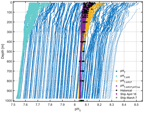
Figure B2A comparison of glider pHT after various corrections have been applied. Raw pHT (blue) is corrected for drift (turquoise) and subsequently for pressure effects (yellow). Finally pHT is compared with “true” ship pHT and corrected (purple). Historical pHT anomalies (black) collected in March and April between 1998 and 2013 are shown for comparison, alongside the ship pHT on 7 March (green squares) and 16 April (pink diamonds).
pHT measurements were corrected for drift using the mean difference (offset) between dive 10 pHT measured between 350 and 950 m and pHT measured at the same depths during each subsequent dive. This method assumes that pHT variations over the 29 d deployment between 350 and 950 m are negligible with respect to the sensor precision. The offsets were added to the full-depth glider pHT profiles, and the range of pHT was reduced 3-fold to approximately 0.3 (Fig. B2).
After correcting pHT for drift, pHT was corrected for pressure using a pressure coefficient of dbar−1. After adding this correction term, the range of pHT was reduced to approximately 0.2 (Fig. B2).
Finally, integrated ISFET pHT values were corrected relative to “true” discrete pHT. Regression coefficients calculated using glider drift- and pressure-corrected pHT and ship pHT collected on 7 March and on 16 April were used to correct glider pHT. The range of glider pHT was now matched with that of historical discrete samples (Fig. B2).
The CO2SYS software package (Van Heuven et al., 2011; Orr et al., 2015) was used to derive discrete pHT for correcting glider ISFET pHT, using discrete measurements of c(DIC), AT, in situ temperature, salinity, pressure, and Si(OH)4 and concentrations. Equilibrium constants (Mehrbach et al., 1973; Dickson and Millero, 1987), sulfate acid dissociation constant (Dickson, 1990) and total borate concentration (Uppström, 1974) were used, as recommended by previous Mediterranean-based studies (Álvarez et al., 2014; Key et al., 2010). c(DIC) and AT had an uncertainty of 3.5 and 3.2 µmol kg−1, respectively, determined from CRM measurements, representing a combined uncertainty of 0.008 in derived pHT.
The AT–S relationship was determined using AT and salinity measurements from discrete ship samples collected in spring 2016 above the salinity maximum (n=20). This parameterisation, (r2=0.88; σ=5.7 µmol kg−1), was used to obtain AT from glider and buoy salinity.
Calibrated glider pHT and AT were used to derive glider f(CO2) and c(DIC) using CO2SYS. The mean uncertainties of derived f(CO2) and c(DIC) were 5.3 µatm and 4.1 µmol kg−1, respectively, calculated as the mean of the absolute differences of f(CO2) and c(DIC) derived using single values of AT and pH (including the margin of error associated with the AT–S relationship and the pHT pressure correction, respectively).
To obtain buoy c(DIC), observed f(CO2) at 10 m was used with AT calculated from S. The uncertainty of derived buoy c(DIC) was 6.6 µmol kg−1, calculated as the absolute difference between the ship c(DIC) sample collected on 7 March at 10 m depth and average c(DIC) measured by the buoy on the same day.
BOUSSOLE buoy data can be found at http://www.obs-vlfr.fr/Boussole/ (Antoine et al., 2022).
Meteorological buoy data are archived in the database “SErvice de DOnnées de l'OMP (SEDOO) Mistrals” (http://mistrals.sedoo.fr/Data-Download, Bouin and Emzivat, 2022).
All glider data are archived at the British Oceanographic Data Centre (BODC, https://doi.org/10.5285/e686816f-8bdd-4782-e053-6c86abc07adc, Kaiser and Hemming, 2022).
This work resulted from MPH's PhD project at the University of East Anglia under the supervision of JK, KJH, DCEB and JB. GAL, MCG and KS implemented the ISFET sensors on the glider and deployed it. JK led the UEA piloting team. DA acquired funding for the Bio-optics and Carbon Experiment (BIOCAREX) that supports the CO2 measurements at BOUSSOLE and led ship operations and ancillary data collection. The data were analysed by MPH and JK, who also wrote the manuscript. All other authors contributed to further editing and writing.
The contact author has declared that none of the authors has any competing interests.
Publisher’s note: Copernicus Publications remains neutral with regard to jurisdictional claims in published maps and institutional affiliations.
This article is part of the special issue “Advances in interdisciplinary studies at multiple scales in the Mediterranean Sea”.
We thank Vincenzo Vellucci, Emilie Diamond and Melek Golbol for monthly sampling at the BOUSSOLE mooring and for aid in planning the 2016 glider deployment. Michael Hemming’s PhD project was funded by the UK Defence Science and Technology Laboratory (DSTL), in cooperation with Direction Générale de l’Armement (DGA, France), with oversight provided by Tim Clarke and Carole Nahum. Ship time on RV Téthys II is provided by the Institut National des Sciences de l'Univers (INSU).
This work was partially funded by the UK National Environment Research Council (NERC; grant nos, NE/K002473/1, NE/N018699/1). BOUSSOLE is funded by the European Space Agency (ESA/ESRIN contracts 4000102992/11/I-NB and 4000111801/14/I-NB) and the Centre National d’Etudes Spatiales (CNES), and this particular study is funded through a grant from the Agence Nationale de la Recherche (ANR, Paris) to the Bio-optics and Carbon Experiment (BIOCAREX).
This paper was edited by Vanessa Cardin and reviewed by three anonymous referees.
Alkire, M. B., D'Asaro, E., Lee, C., Perry, M. J., Gray, A., Cetinić, I., Briggs, N., Rehm, E., Kallin, E., Kaiser, J., and González-Posada, A.: Estimates of net community production and export using high-resolution, Lagrangian measurements of O2, NO3−, and POC through the evolution of a spring diatom bloom in the North Atlantic, Deep Sea Res. Pt. I, 64, 157–174, 2012. a
Alkire, M. B., Lee, C., D'Asaro, E., Perry, M. J., Briggs, N., Cetinić, I., and Gray, A.: Net community production and export from Seaglider measurements in the North Atlantic after the spring bloom, J. Geophys. Res.-Oceans, 119, 6121–6139, 2014. a, b, c, d, e
Álvarez, M., Sanleón-Bartolomé, H., Tanhua, T., Mintrop, L., Luchetta, A., Cantoni, C., Schroeder, K., and Civitarese, G.: The CO2 system in the Mediterranean Sea: a basin wide perspective, Ocean Sci., 10, 69–92, https://doi.org/10.5194/os-10-69-2014, 2014. a, b
Anderson, L. A.: On the hydrogen and oxygen content of marine phytoplankton, Deep Sea Res. Pt. I, 42, 1675–1680, 1995. a
Anderson, L. A. and Sarmiento, J. L.: Global ocean phosphate and oxygen simulations, Global Biogeochem. Cy., 9, 621–636, 1995. a
Antoine, D., d'Ortenzio, F., Hooker, S. B., Bécu, G., Gentili, B., Tailliez, D., and Scott, A. J.: Assessment of uncertainty in the ocean reflectance determined by three satellite ocean color sensors (MERIS, SeaWiFS and MODIS-A) at an offshore site in the Mediterranean Sea (BOUSSOLE project), J. Geophys. Res.-Oceans, 113, C07013, https://doi.org/10.1029/2007JC004472, 2008. a
Antoine, D., Vellucci, V., Golbol, M., and Gentili, B.: BOUSSOLE buoy data, http://www.obs-vlfr.fr/Boussole/, last access: 20 August 2022. a
Arrigo, K. R., van Dijken, G. L., and Bushinsky, S.: Primary production in the Southern Ocean, 1997–2006, J. Geophys. Res.-Oceans, 113, C08004, https://doi.org/10.1029/2007jc004551, 2008. a
Bauer, J. E., Cai, W.-J., Raymond, P. A., Bianchi, T. S., Hopkinson, C. S., and Regnier, P. A.: The changing carbon cycle of the coastal ocean, Nature, 504, 61–70, 2013. a
Bendschneider, K. and Robinson, R. J.: A new spectrophotometric method for the determination of nitrite in sea water, J. Mar. Res., http://hdl.handle.net/1773/15938, 1952. a
Benson, B. B. and Krause, D.: The concentration and isotopic fractionation of oxygen dissolved in fresh water and seawater in equilibrium with the atmosphere, Limnol. Oceanogr., 29, 620–632, https://doi.org/10.4319/lo.1984.29.3.0620, 1984. a
Binetti, U., Kaiser, J., Damerell, G., Rumyantseva, A., Martin, A., Henson, S., and Heywood, K.: Net community oxygen production derived from Seaglider deployments at the Porcupine Abyssal Plain site (PAP; northeast Atlantic) in 2012–13, Prog. Oceanogr., 183, 102293, https://doi.org/10.1016/j.pocean.2020.102293, 2020. a, b, c
Bonjean, F. and Lagerloef, G. S.: Diagnostic model and analysis of the surface currents in the tropical Pacific Ocean, J. Phys. Oceanogr., 32, 2938–2954, 2002. a
Bouin, M.-N. and Emzivat, G.: SErvice de DOnnées de l’OMP (SEDOO) Mistrals, Sedoo [data set], http://mistrals.sedoo.fr/Data-Download, last access: 20 August 2022. a
Brainerd, K. E. and Gregg, M. C.: Surface mixed and mixing layer depths, Deep Sea Res. Pt. I, 42, 1521–1543, https://doi.org/10.1016/0967-0637(95)00068-H, 1995. a
Bresnahan, P. J., Martz, T. R., Takeshita, Y., Johnson, K. S., and LaShomb, M.: Best practices for autonomous measurement of seawater pH with the Honeywell Durafet, Methods Oceanogr., 9, 44–60, 2014. a
Broecker, W. S., Takahashi, T., Simpson, H., and Peng, T.-H.: Fate of fossil fuel carbon dioxide and the global carbon budget, Science, 206, 409–418, 1979. a
Carlson, C. A., Ducklow, H. W., Hansell, D. A., and Smith, W. O.: Organic carbon partitioning during spring phytoplankton blooms in the Ross Sea polynya and the Sargasso Sea, Limnol. Oceanogr., 43, 375–386, 1998. a, b
Copin-Montégut, C.: Consumption and production on scales of a few days of inorganic carbon, nitrate and oxygen by the planktonic community: results of continuous measurements at the Dyfamed Station in the northwestern Mediterranean Sea (May 1995), Deep Sea Res. Pt. I, 47, 447–477, 2000. a, b, c, d, e, f, g, h, i
Copin-Montégut, C. and Bégovic, M.: Distributions of carbonate properties and oxygen along the water column (0–2000m) in the central part of the NW Mediterranean Sea (Dyfamed site): influence of winter vertical mixing on air–sea CO2 and O2 exchanges, Deep Sea Res. Pt. II, 49, 2049–2066, 2002. a
Copin-Montégut, C., Bégovic, M., and Merlivat, L.: Variability of the partial pressure of CO2 on diel to annual time scales in the Northwestern Mediterranean Sea, Mar. Chem., 85, 169–189, 2004. a, b, c, d, e, f
Coppola, L., Legendre, L., Lefevre, D., Prieur, L., Taillandier, V., and Riquier, E. D.: Seasonal and inter–annual variations of dissolved oxygen in the northwestern Mediterranean Sea (DYFAMED site), Prog. Oceanogr., 162, 187–201, https://doi.org/10.1016/j.pocean.2018.03.001, 2018. a, b, c, d, e
Cornwall, C. E., Hepburn, C. D., McGraw, C. M., Currie, K. I., Pilditch, C. A., Hunter, K. A., Boyd, P. W., and Hurd, C. L.: Diurnal fluctuations in seawater pH influence the response of a calcifying macroalga to ocean acidification, P. Roy. Soc. London B, 280, 20132201, https://doi.org/10.1098/rspb.2013.2201, 2013. a
Cuypers, Y., Bouruet-Aubertot, P., Marec, C., and Fuda, J.-L.: Characterization of turbulence from a fine-scale parameterization and microstructure measurements in the Mediterranean Sea during the BOUM experiment, Biogeosciences, 9, 3131–3149, https://doi.org/10.5194/bg-9-3131-2012, 2012. a, b
Cyr, F., Tedetti, M., Besson, F., Beguery, L., Doglioli, A. M., Petrenko, A. A., and Goutx, M.: A new glider-compatible optical sensor for dissolved organic matter measurements: test case from the NW Mediterranean Sea, Front. Mar. Sci., 4, 89, https://doi.org/10.3389/fmars.2017.00089, 2017. a
de Fommervault, O. P., Migon, C., d'Alcalà, M. R., and Coppola, L.: Temporal variability of nutrient concentrations in the northwestern Mediterranean sea (DYFAMED time-series station), Deep Sea Res. Pt. I, 100, 1–12, https://doi.org/10.1002/2015JC011103, 2015. a, b
Dickson, A. and Millero, F. J.: A comparison of the equilibrium constants for the dissociation of carbonic acid in seawater media, Deep Sea Res. Pt. A, 34, 1733–1743, 1987. a
Dickson, A. G.: Thermodynamics of the dissociation of boric acid in synthetic seawater from 273.15 to 318.15 K, Deep Sea Res. Pt. A, 37, 755–766, 1990. a
Dickson, A. G., Sabine, C. L., and Christian, J. R. (Eds.): Guide to best practices for ocean CO2 measurements, PICES Special Publication 3, 191 pp., “Guide” in one PDF file, https://www.ncei.noaa.gov/access/ocean-carbon-acidification-data-system/oceans/Handbook_2007.html (last access: 24 August 2022), 2007. a, b
Dlugokencky, E. J., Mund, J. W., Crotwell, A. M., Crotwell, M. J., and Thoning, K. W.: Atmospheric carbon dioxide dry air mole fractions from the NOAA GML carbon cycle cooperative global air sampling network, 1968–2020, Version: 2021-07-30, https://doi.org/10.15138/wkgj-f215, 2021. a
D’Ortenzio, F., Antoine, D., and Marullo, S.: Satellite-driven modeling of the upper ocean mixed layer and air–sea CO2 flux in the Mediterranean Sea, Deep Sea Res. Pt. I, 55, 405–434, 2008. a
Eriksen, C. C., Osse, T. J., Light, R. D., Wen, T., Lehman, T. W., Sabin, P. L., Ballard, J. W., and Chiodi, A. M.: Seaglider: A long-range autonomous underwater vehicle for oceanographic research, Ocean Engineering, IEEE Journal of Oceanic Engineering, 26, 424–436, https://doi.org/10.1109/48.972073, 2001. a
Estrada, M.: Primary production in the northwestern Mediterranean, Scientia Marina, 60, 55–64, 1996. a
Friedlingstein, P., Jones, M. W., O'Sullivan, M., Andrew, R. M., Bakker, D. C. E., Hauck, J., Le Quéré, C., Peters, G. P., Peters, W., Pongratz, J., Sitch, S., Canadell, J. G., Ciais, P., Jackson, R. B., Alin, S. R., Anthoni, P., Bates, N. R., Becker, M., Bellouin, N., Bopp, L., Chau, T. T. T., Chevallier, F., Chini, L. P., Cronin, M., Currie, K. I., Decharme, B., Djeutchouang, L. M., Dou, X., Evans, W., Feely, R. A., Feng, L., Gasser, T., Gilfillan, D., Gkritzalis, T., Grassi, G., Gregor, L., Gruber, N., Gürses, Ö., Harris, I., Houghton, R. A., Hurtt, G. C., Iida, Y., Ilyina, T., Luijkx, I. T., Jain, A., Jones, S. D., Kato, E., Kennedy, D., Klein Goldewijk, K., Knauer, J., Korsbakken, J. I., Körtzinger, A., Landschützer, P., Lauvset, S. K., Lefèvre, N., Lienert, S., Liu, J., Marland, G., McGuire, P. C., Melton, J. R., Munro, D. R., Nabel, J. E. M. S., Nakaoka, S.-I., Niwa, Y., Ono, T., Pierrot, D., Poulter, B., Rehder, G., Resplandy, L., Robertson, E., Rödenbeck, C., Rosan, T. M., Schwinger, J., Schwingshackl, C., Séférian, R., Sutton, A. J., Sweeney, C., Tanhua, T., Tans, P. P., Tian, H., Tilbrook, B., Tubiello, F., van der Werf, G. R., Vuichard, N., Wada, C., Wanninkhof, R., Watson, A. J., Willis, D., Wiltshire, A. J., Yuan, W., Yue, C., Yue, X., Zaehle, S., and Zeng, J.: Global Carbon Budget 2021, Earth Syst. Sci. Data, 14, 1917–2005, https://doi.org/10.5194/essd-14-1917-2022, 2022. a
García, H. E. and Gordon, L. I.: Oxygen solubility in seawater: Better fitting equations, Limnol. Oceanogr., 37, 1307–1312, 1992. a, b
Gross, A. M.: Confidence intervals for bisquare regression estimates, J. Am. Stat. Assoc., 72, 341–354, 1977. a
Hall, T. M., Waugh, D. W., Haine, T. W., Robbins, P. E., and Khatiwala, S.: Estimates of anthropogenic carbon in the Indian Ocean with allowance for mixing and time-varying air-sea CO2 disequilibrium, Global Biogeochem. Cy., 18, GB1031, https://doi.org/10.1029/2003GB002120, 2004. a
Hemming, M. P., Kaiser, J., Heywood, K. J., Bakker, D. C. E., Boutin, J., Shitashima, K., Lee, G., Legge, O., and Onken, R.: Measuring pH variability using an experimental sensor on an underwater glider, Ocean Sci., 13, 427–442, https://doi.org/10.5194/os-13-427-2017, 2017. a, b, c, d, e, f, g, h
Holte, J. and Talley, L.: A new algorithm for finding mixed layer depths with applications to Argo data and subantarctic mode water formation, J. Atmos. Ocean. Tech., 26, 1920–1939, 2009. a, b
Hood, E. and Merlivat, L.: Annual to interannual variations of fCO2 in the northwestern Mediterranean Sea: Results from hourly measurements made by CARIOCA buoys, 1995–1997, J. Mar. Res., 59, 113–131, 2001. a, b, c
Hu, C., Lee, Z., and Franz, B.: Chlorophyll a algorithms for oligotrophic oceans: A novel approach based on three-band reflectance difference, J. Geophys. Res.-Oceans, 117, C01011, https://doi.org/10.1029/2011JC007395, 2012. a
Hull, T., Greenwood, N., Birchill, A., Beaton, A., Palmer, M., and Kaiser, J.: Simultaneous assessment of oxygen- and nitrate-based net community production in a temperate shelf sea from a single ocean glider, Biogeosciences, 18, 6167–6180, https://doi.org/10.5194/bg-18-6167-2021, 2021. a, b
Johnson, K. M., King, A. E., and Sieburth, J. M.: Coulometric TCO2 analyses for marine studies; an introduction, Mar. Chem., 16, 61–82, 1985. a
Kaiser, J. and Hemming, M. P.: Deployment of UEA Seaglider sg537 ('Fin') near the Boussole time series site (Mediterranean Sea) with pH/p(CO2) ISFET sensor testing, March–April 2016, NERC EDS British Oceanographic Data Centre NOC [data set], https://doi.org/10.5285/e686816f-8bdd-4782-e053-6c86abc07adc, 2022. a
Key, R. M., Tanhua, T., Olsen, A., Hoppema, M., Jutterström, S., Schirnick, C., van Heuven, S., Kozyr, A., Lin, X., Velo, A., Wallace, D. W. R., and Mintrop, L.: The CARINA data synthesis project: introduction and overview, Earth Syst. Sci. Data, 2, 105–121, https://doi.org/10.5194/essd-2-105-2010, 2010. a
Knoll, M., Borrione, I., Fiekas, H.-V., Funk, A., Hemming, M. P., Kaiser, J., Onken, R., Queste, B., and Russo, A.: Hydrography and circulation west of Sardinia in June 2014, Ocean Sci., 13, 889–904, https://doi.org/10.5194/os-13-889-2017, 2017. a
Laws, E. A.: Photosynthetic quotients, new production and net community production in the open ocean, Deep Sea Res. Pt. A, 38, 143–167, 1991. a
Lee, K., Sabine, C. L., Tanhua, T., Kim, T.-W., Feely, R. A., and Kim, H.-C.: Roles of marginal seas in absorbing and storing fossil fuel CO2, Energ. Environ. Sci., 4, 1133–1146, 2011. a
Lee, Z., Weidemann, A., Kindle, J., Arnone, R., Carder, K. L., and Davis, C.: Euphotic zone depth: Its derivation and implication to ocean-color remote sensing, J. Geophys. Res.-Oceans, 112, C03009, https://doi.org/10.1029/2006JC003802, 2007. a
Marty, J.-C. and Chiavérini, J.: Seasonal and interannual variations in phytoplankton production at DYFAMED time-series station, northwestern Mediterranean Sea, Deep Sea Res. Pt. II, 49, 2017–2030, 2002. a
McNeil, C. L. and D'Asaro, E. A.: A calibration equation for oxygen optodes based on physical properties of the sensing foil, Limnol. Oceanogr., 12, 139–154, 2014. a
Mehrbach, C., Culberson, C., Hawley, J., and Pytkowics, R.: Measurement of the apparent dissociation constants of carbonic acid in seawater at atmospheric pressure, Limnol. Oceanogr., 18, 897–907, https://doi.org/10.4319/lo.1973.18.6.0897, 1973. a
Merlivat, L., Boutin, J., Antoine, D., Beaumont, L., Golbol, M., and Vellucci, V.: Increase of dissolved inorganic carbon and decrease in pH in near-surface waters in the Mediterranean Sea during the past two decades, Biogeosciences, 15, 5653–5662, https://doi.org/10.5194/bg-15-5653-2018, 2018. a, b, c, d
Murphy, J. and Riley, J. P.: A modified single solution method for the determination of phosphate in natural waters, Anal. Chim. Acta, 27, 31–36, 1962. a
Niewiadomska, K., Claustre, H., Prieur, L., and d'Ortenzio, F.: Submesoscale physical-biogeochemical coupling across the Ligurian current (northwestern Mediterranean) using a bio-optical glider, Limnol. Oceanogr., 53, 2210–2225, 2008. a
Onken, R., Fiekas, H.-V., Beguery, L., Borrione, I., Funk, A., Hemming, M., Hernandez-Lasheras, J., Heywood, K. J., Kaiser, J., Knoll, M., Mourre, B., Oddo, P., Poulain, P.-M., Queste, B. Y., Russo, A., Shitashima, K., Siderius, M., and Thorp Küsel, E.: High-resolution observations in the western Mediterranean Sea: the REP14-MED experiment, Ocean Sci., 14, 321–335, https://doi.org/10.5194/os-14-321-2018, 2018. a, b
Orr, J. C., Epitalon, J.-M., and Gattuso, J.-P.: Comparison of ten packages that compute ocean carbonate chemistry, Biogeosciences, 12, 1483–1510, https://doi.org/10.5194/bg-12-1483-2015, 2015. a
Pingree, R., Maddock, L., and Butler, E.: The influence of biological activity and physical stability in determining the chemical distributions of inorganic phosphate, silicate and nitrate, J. Mar. Biol. Assoc. UK, 57, 1065–1073, 1977. a
Piterbarg, L., Taillandier, V., and Griffa, A.: Investigating frontal variability from repeated glider transects in the Ligurian Current (North West Mediterranean Sea), J. Mar. Syst., 129, 381–395, 2014. a
Queste, B. Y., Heywood, K. J., Kaiser, J., Lee, G., Matthews, A., Schmidtko, S., Walker-Brown, C., and Woodward, S. W.: Deployments in extreme conditions: Pushing the boundaries of Seaglider capabilities, in: Autonomous Underwater Vehicles (AUV), 2012 IEEE/OES, pp. 1–7, IEEE, 2012. a
Redfield, A., Ketchum, B., and Richards, F.: The influence of organisms on the composition of seawater, The Sea, 2, 26–77, 1963. a
Roquet, F., Madec, G., McDougall, T. J., and Barker, P. M.: Accurate polynomial expressions for the density and specific volume of seawater using the TEOS-10 standard, Ocean Model., 90, 29–43, 2015. a
Saba, G. K., Wright-Fairbanks, E., Miles, T. N., Chen, B., Cai, W.-J., Wang, K., Barnard, A. H., Branham, C. W., and Jones, C. P.: Developing a profiling glider pH sensor for high resolution coastal ocean acidification monitoring, in: OCEANS 2018 MTS/IEEE Charleston, pp. 1–8, IEEE, 2018. a
Schneider, A., Tanhua, T., Körtzinger, A., and Wallace, D. W.: High anthropogenic carbon content in the eastern Mediterranean, J. Geophys. Res.-Oceans, 115, C12050, https://doi.org/10.1029/2010JC006171, 2010. a
Shitashima, K., Maeda, Y., and Ohsumi, T.: Development of detection and monitoring techniques of CO2 leakage from seafloor in sub-seabed CO2 storage, Appl. Geochem., 30, 114–124, 2013. a
Stramski, D., Boss, E., Bogucki, D., and Voss, K. J.: The role of seawater constituents in light backscattering in the ocean, Prog. Oceanogr., 61, 27–56, 2004. a
Strickland, J. D. and Parsons, T. R.: A practical handbook of seawater analysis, Fisheries Research Board of Canada, https://publications.gc.ca/pub?id=9.581564&sl=0 (last access: 24 August 2022), 1972. a
Sverdrup, H.: On vernal blooming of phytoplankton, J. Conseil Exp. Mer, 18, 287–295, 1953. a
Taillandier, V., D'Ortenzio, F., and Antoine, D.: Carbon fluxes in the mixed layer of the Mediterranean Sea in the 1980s and the 2000s, Deep Sea Res. Pt. I, 65, 73–84, https://doi.org/10.1016/j.dsr.2012.03.004, 2012. a
Takahashi, T., Olafsson, J., Goddard, J. G., Chipman, D. W., and Sutherland, S.: Seasonal variation of CO2 and nutrients in the high-latitude surface oceans: A comparative study, Global Biogeochem. Cy., 7, 843–878, 1993. a
Takahashi, T., Sutherland, S. C., Sweeney, C., Poisson, A., Metzl, N., Tilbrook, B., Bates, N., Wanninkhof, R., Feely, R. A., Sabine, C., Olafsson, J., and Nojiri, Y.: Global sea–air CO2 flux based on climatological surface ocean pCO2, and seasonal biological and temperature effects, Deep Sea Res. Pt. II, 49, 1601–1622, https://doi.org/10.1016/S0967-0645(02)00003-6, 2002. a
Takeshita, Y., Martz, T. R., Johnson, K. S., and Dickson, A. G.: Characterization of an ion sensitive field effect transistor and chloride ion selective electrodes for pH measurements in seawater, Anal. Chem., 86, 11189–11195, 2014. a
Takeshita, Y., Jones, B. D., Johnson, K. S., Chavez, F. P., Rudnick, D. L., Blum, M., Conner, K., Jensen, S., Long, J. S., Maughan, T., Mertz, K. L., Sherman, J. T., and Warren, J. K.: Accurate pH and O2 measurements from spray underwater gliders, J. Atmos. Ocean. Tech., 38, 181–195, 2021. a
Uppström, L. R.: The boron/chlorinity ratio of deep-sea water from the Pacific Ocean, Deep Sea Res. Ocean. Abstr., 21, 161–162, 1974. a
Van Der Loeff, M. M. R., Friedrich, J., and Bathmann, U. V.: Carbon export during the spring bloom at the Antarctic Polar Front, determined with the natural tracer 234 Th, Deep Sea Res. Pt. II, 44, 457–478, 1997. a
Van Heuven, S., Pierrot, D., Rae, J., Lewis, E., and Wallace, D.: MATLAB program developed for CO2 system calculations, ORNL/CDIAC-105b, Carbon Dioxide Inf, Anal. Cent., Oak Ridge Natl. Lab., US DOE, Oak Ridge, Tennessee, 2011. a
Wanninkhof, R.: Relationship between wind speed and gas exchange over the ocean revisited, Limnol. Oceanogr. Methods, 12, 351–362, 2014. a, b
Wanninkhof, R. and Thoning, K.: Measurement of fugacity of CO2 in surface water using continuous and discrete sampling methods, Mar. Chem., 44, 189–204, 1993. a
Weiss, R. and Price, B.: Nitrous oxide solubility in water and seawater, Mar. Chem., 8, 347–359, 1980. a
Woolf, D. K. and Thorpe, S.: Bubbles and the air-sea exchange of gases in near-saturation conditions, J. Mar. Res., 49, 435–466, 1991. a
Yao, K. M., Marcou, O., Goyet, C., Guglielmi, V., Touratier, F., and Savy, J.-P.: Time variability of the north-western Mediterranean Sea pH over 1995–2011, Mar. Environ. Res., 116, 51–60, 2016. a
Zeebe, R. E. and Wolf-Gladrow, D. A. (Eds.): CO2 in seawater: equilibrium, kinetics, isotopes, Elsevier, vol. 65, 346 pp., ISBN 978-0-444-50579-8, 2001. a
- Abstract
- Introduction
- Data collection and quality
- Development of a spring bloom
- Estimating net community production from O2 and DIC mass budgets
- Net community production N
- Stoichiometric relationship
- Discussion
- Conclusions
- Appendix A: Discrete water samples
- Appendix B: Glider calibrations
- Appendix C: Deriving parameters using CO2SYS
- Data availability
- Author contributions
- Competing interests
- Disclaimer
- Special issue statement
- Acknowledgements
- Financial support
- Review statement
- References