Compound flooding in convergent estuaries: insights from an analytical model

We investigate here the effects of geometric properties (channel depth and cross-sectional convergence length), storm surge characteristics, friction, and river flow on the spatial and temporal variability of compound flooding along an idealized, meso-tidal coastal-plain estuary. An analytical model is developed that includes exponentially convergent geometry, tidal forcing, constant river flow, and a representation of storm surge as a combination of two sinusoidal waves. Nonlinear bed friction is treated using Chebyshev polynomials and trigonometric functions, and a multi-segment approach is used to increase accuracy. Model results show that river discharge increases the damping of surge amplitudes in an estuary, while increasing channel depth has the opposite effect. Sensitivity studies indicate that the impact of river flow on peak water level decreases as channel depth increases, while the influence of tide and surge increases in the landward portion of an estuary. Moreover, model results show less surge damping in deeper configurations and even amplification in some cases, while increased convergence length scale increases damping of surge waves with periods of 12–72 h. For every modeled scenario, there is a point where river discharge effects on water level outweigh tide/surge effects. As a channel is deepened, this cross-over point moves progressively upstream. Thus, channel deepening may alter flood risk spatially along an estuary and reduce the length of a river estuary, within which fluvial flooding is dominant.

1 Introduction

Understanding tidal, surge, and river flow dynamics and how they combine and interact to produce the maximum or total water level (TWL) is important for emergency planning and as an aspect of wave dynamics. It is also a problem that is changing rapidly, as sea level rises and systems are altered by engineering. This contribution therefore analyzes the relative influence of river flow and storm surge effects along the river–estuary continuum from a dynamical perspective that enables us to assess the effects of nonlinear interactions, geometry, and changing (time varying) conditions.

Many low-lying coastal and riverine areas have been affected by combined coastal and riverine floods over the last few decades (e.g., Jongman et al., 2012; Nicholls et al., 2007). In cases such as Hurricane Harvey (Gulf of Mexico, August 2017), flooding was driven primarily by precipitation and runoff (van Oldenborgh et al., 2017; Wang et al., 2018). Other flood events, such as Hurricane Sandy, were forced by the combined effects of tide and storm surge, i.e., by “storm tides” the sum of storm surge and tidal water level (Orton et al., 2016). Some storm events, like Hurricanes Irene and Irma, produce both coastal and inland flooding because both storm surge and river flow produce elevated coastal water levels in a spatially varying pattern (e.g., Orton et al., 2012; Ralston et al., 2013; Talke et al., 2021). Accordingly, a flood influenced by both storm tide and precipitation run-off is a “compound flood” (Zscheischler et al., 2018; Wahl et al., 2015). The relative timing of the coastal and fluvial forcing, and the timescale over which water levels are elevated, matters in terms of impact (e.g., Zheng et al., 2014). Storm surge flooding generally occurs first and for a shorter period (timescales of hours to a day or two) than river flooding, which may last for weeks or even months, particularly in regions with a large watershed and flat topography (e.g., Johnson et al., 2016; IPCC, 2014). The timing of storm surge relative to tidal high-water (Familkhalili and Talke, 2016) or the spring–neap tidal cycle also influences flood heights, even upstream of tidal influence (Helaire et al., 2020).

The spatial variability of compound flooding is influenced by the geometry of an estuary and may change over time due to system alterations, including channel deepening, sea-level rise, and wetland reclamation (Ralston et al., 2019; Helaire et al., 2019, 2020). Recent studies have shown that human-caused changes to the geometry of estuaries affect the dynamics of long waves (see reviews by Talke and Jay, 2020; Jay et al., 2022), with tidal range in some regions more than doubling (e.g., Winterwerp et al., 2013). Similar effects are observed with storm surge; for example, doubling the depth of the shipping channel in the Cape Fear Estuary was modeled to increase the magnitude of a worst-case scenario storm surge in Wilmington (NC) from 3.8 ± 0.25 to 5.6 ± 0.6 m (Familkhalili and Talke, 2016). By contrast, depth increases may cause the mean water level in tidal rivers to drop due to decreased frictional effects (Jay et al., 2011; Helaire et al., 2019); hence, flood risk in Albany (NY) has significantly dropped over the past 150 years, despite a doubling of tide range and an increase in storm surge magnitudes (Ralston et al., 2019). Closer to the coast, flood hazard within the same estuary markedly increased over the same time period (e.g., Talke et al., 2014). Hence, evolution of flood hazard can be spatially variable to an extent that is just beginning to be quantified.

Here, an idealized approach is used, which enables a large parameter space to be assessed and the following two dynamical questions to be investigated.

• a.

  What factors determine the region in which river flow effects or tide and surge effects dominate the total water level?

• b.

  How does the transition from coastal to fluvial dominance shift as geometry changes or as properties of storm surge (e.g., timescale and magnitude) and river flow (magnitude) change?

We combine a three-sinusoidal-wave analytical model based on Jay (1991) with the multi-wave and multi-segment approach of Giese and Jay (1989) (see Familkhalili et al., 2020 for details) to quickly query a parameter space or relevant factors and provide insight into how factors such as storm timescale and the relative magnitudes of different forcing factors influence the dynamics of compound flooding.

2 Methods

Both analytical solutions and numerical models are regularly used to explore the mechanism of surge and tidal waves propagation along an estuary (see Talke and Jay, 2020). While numerical models can simulate tidal wave propagation more accurately than analytical models considering the measurements in a real system, numerical models are typically calibrated for an existing bathymetric, meteorological, and boundary forcing configurations (e.g., Brandon et al., 2014; Bertin et al., 2012; Orton et al., 2012). On the other hand, idealized numerical models with simplified configurations can be used to develop sensitivity studies to investigate the effects of changing hydrodynamic variables on surge and tidal wave interactions in a system (e.g., Shen and Gong, 2009; Familkhalili and Talke, 2016), but a downside of these numerical approaches is that studying an entire parameter space is computationally expensive. In contrast, analytical models rely on fundamental underlying physics and are transparent. Thus, they are good tools to explain some of the factors (e.g., channel depth, convergence length, river discharge, and surge amplitude and timescale changes) that alter flood levels in an estuary.

We apply an analytical approach to investigate the TWL caused by river discharge, tides, and surge in an idealized estuary. Various forms of one-dimensional analytical solutions of tidal wave propagation have long been used for idealized and real estuaries (e.g., Dronkers, 1964; Prandle and Rahman, 1980; Jay, 1991; Friedrichs and Aubrey, 1994; Savenije, 1998; Lanzoni and Seminara, 1998; Godin, 1999). More complex idealized tidal models investigate overtide generation and evolution (e.g., Chernetsky et al., 2010), the effects of variable cross section and bottom slope (e.g., Savenije et al., 2008; Kästner et al., 2019), and the effects of multiple tidal constituents and river discharge (Giese and Jay, 1989; Buschman et al., 2009). Other studies have used a tidal model combined with regression analysis (e.g., Godin, 1999; Kukulka and Jay, 2003a) to investigate river discharge effects. Such idealized models, by the parameter space analyzed, can be used to obtain fundamental insights into how long waves in estuaries are affected by depth, convergence, friction, and boundary forcing.

In our approach, we develop an analytical model that is driven by three sinusoidal constituents and a constant river discharge. Our approach idealizes storm surge as the sum of two sinusoids and neglects factors such as the potential role of wetlands and the floodplain in order to gain insight into some of the important, along-channel factors that govern the system response to a compound event. Similarly, we neglect processes such as Coriolis acceleration, wind waves, and gravity waves, and focus on the specific case of an incident long wave that propagates from the coast in the landward direction and is eventually completely damped out. Though a reflected wave is produced by convergent geometry in analytical models (Jay, 1991), we neglect the partial reflections caused by depth and width changes and do not consider the case of a reflective upstream boundary. Such factors are important for tidal changes in many estuaries, particularly for locations that are near resonance such as the Ems (see Ensing et al., 2015) or near where total reflections occur (see Ralston et al., 2019). Moreover, we simplify our approach by considering only constant river flow conditions, a valid approximation for situations in which the timescale of a river flood event is much longer than a storm surge. These simplifications enable a solution that is much faster than numerical models and enables a tractable sensitivity study of storm surge and river flow effects on water levels for different depths, convergence, and boundary conditions.

2.1 Analytical model

We use an idealized one-dimensional analytical model developed by Familkhalili et al. (2020) to investigate how combinations of tides, storm surge, and river flow affect water levels in an estuary. In this model, storm surge is approximated as the sum of a primary and a secondary sinusoidal wave. A third sinusoidal frequency is reserved for the M₂ tidal constituent. The resulting model is conceptually similar to the multi-tide constituent model developed by Giese and Jay (1989) and the three-wave model of Buschman et al. (2009), with the distinction that two of the waves are based on the amplitude and timescales of meteorologically induced storm surge rather than an astronomical tide with a known frequency. In addition, the Giese and Jay (1989) model used the dynamical analysis of Dronkers (1964), which does not correctly include convergence effects, whereas our model follows the Jay (1991) treatment, which includes friction, convergence, and river inflow.

One-dimensional long-wave propagation along an idealized, funnel-shaped estuary is described by the cross-sectionally integrated equations of mass and momentum conservation (e.g., Jay, 1991; Kukulka and Jay, 2003a; Familkhalili et al., 2020):

$$\begin{array}{}\text{(1)}& {\displaystyle \frac{\partial Q}{\partial t}}+{\displaystyle \frac{\partial }{\partial x}}\left({\displaystyle \frac{Q^{\mathrm{2}}}{A}}\right)+gA{\displaystyle \frac{\partial \mathit{\xi }}{\partial x}}+bK=\mathrm{0},\text{(2)}& {\displaystyle \frac{\partial Q}{\partial x}}+b{\displaystyle \frac{\partial \mathit{\xi }}{\partial t}}=\mathrm{0},\end{array}$$

where Q is cross-sectionally integrated flow (m³ s⁻¹) and is the summation of the river and tidal transports (Q_R+ Q_T), t is time (s), x is the longitudinal coordinate measured in landward direction (m) (see Fig. 1a), b is width (m), g is the acceleration due to gravity (9.81 m s⁻²), A is channel cross-sectional area (m²), ξ is tidal amplitude (m), K is the bed stress divided by water density (m² s⁻²) ($\frac{\mathit{\tau }}{\mathit{\rho }}=C_{\mathrm{d}}\left|u\right|u$), C_d is a dimensionless drag coefficient, and $u=Q/A$ is the velocity (m s⁻¹). The absolute value of u is assigned to preserve the directionality of stress. For simplicity, depth is assumed constant and channel width is allowed to vary exponentially with respect to the longitudinal coordinate x (i.e., $b_{\left(x\right)}=B_{\mathrm{c}}+(B_{\mathrm{0}}-B_{\mathrm{c}})e^{\left(-\frac{x}{L_{\mathrm{e}}}\right)}$, see Fig. 1a), where B₀ is the width at the estuary mouth (m) and B_c is the constant upstream river width (m) and L_e is the convergence length scale (m) that is the length over which the width decreases by a factor of e. Following Familkhalili et al. (2020), we set B₀=5 km and assume that the estuary section of the model domain is 1.5 times the convergence length, which determines a constant river width of ∼ 1100 m. The constant depth channel is routed upstream for 100 km to enable the tide wave to dissipate and prevent reflection off an upstream boundary. The tidal amplitude to depth ratio ($\frac{\mathit{\xi }}{h}$) is assumed small, and river flow (Q_R) is held constant (e.g., Kukulka and Jay, 2003a; Familkhalili et al., 2020). Applying these assumptions and combining Eqs. (1) and (2) yields the following differential equation:

$$\begin{array}{}\text{(3)}& \begin{array}{rl}{\displaystyle \frac{{\partial }^{\mathrm{2}}{Q}_{\mathrm{T}}}{\partial x^{\mathrm{2}}}}& -{\displaystyle \frac{\mathrm{1}}{b}}{\displaystyle \frac{\partial b}{\partial x}}{\displaystyle \frac{\partial Q_{\mathrm{T}}}{\partial x}}-\mathrm{2}{\displaystyle \frac{\mathrm{1}}{gh}}{U}_{\mathrm{R}}{\displaystyle \frac{{\partial }^{\mathrm{2}}{Q}_{\mathrm{T}}}{\partial x\partial t}}\\ & +\mathrm{2}{\displaystyle \frac{\mathrm{1}}{gh}}{U}_{\mathrm{R}}{\displaystyle \frac{\mathrm{1}}{A}}{\displaystyle \frac{\partial A}{\partial x}}{\displaystyle \frac{\partial Q_{\mathrm{T}}}{\partial t}}-{\displaystyle \frac{\mathrm{1}}{gh}}{\displaystyle \frac{{\partial }^{\mathrm{2}}{Q}_{\mathrm{T}}}{\partial t^{\mathrm{2}}}}\\ & -{\displaystyle \frac{b}{gh}}{\displaystyle \frac{\partial K}{\partial t}}=\mathrm{0}\end{array}.\end{array}$$

We linearize the frictional term (K=C_d|u|u) using Chebyshev polynomials (Dronkers, 1964) to approximate the frictional term, u|u|. Following Godin (1991, 1999), only the first- and third-order terms of the dimensionless velocity are retained, yielding

$$\begin{array}{}\text{(4)}& {\displaystyle \frac{u\left|u\right|}{U_{\left(x\right)}^{\mathrm{2}}}}\approx A{u}^{\prime }+B{u^{\prime }}^{\mathrm{3}},\end{array}$$

where $A=\frac{\mathrm{16}}{\mathrm{15}\mathit{\pi }}$, $B=\frac{\mathrm{32}}{\mathrm{15}\mathit{\pi }}$, U_(x) is a function of x and is the maximum value of the total current (U_R+U_T), where U_R and U_T are maximum river and tidal velocity, respectively, and u^′ is a non-dimensionalized velocity defined as $\frac{u}{\left|U_{\left(x\right)}\right|}$ (Doodson, 1956; Godin, 1991). See Familkhalili et al. (2020) for additional details.

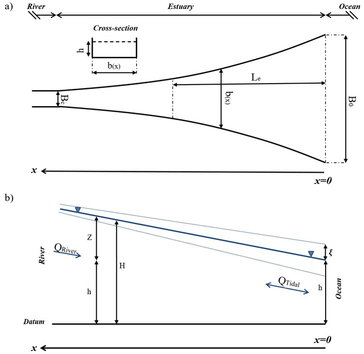
Figure 1 (a) Idealized bathymetry and plan view of the conceptual model and (b) definition of the water surface slope, modified from Kukulka and Jay (2003b). The along-channel direction x is upstream, with x=0 being at the ocean. The convergent section of the model domain is 1.5 times the convergence length, and the river channel at the left-hand side extends an additional 100 km to enable tidal and surge constituents to damp out. See Appendix A for a description of parameters.

The sectionally and vertically averaged velocity term in Eq. (3) ($u=Q/A)$ is decomposed into three sinusoidal wave components and a constant river discharge:

$$\begin{array}{}\text{(5)}& u=-u_{\mathrm{r}}+\sum _{i=\mathrm{1}}^{\mathrm{3}}{u}_i\cos \left({\mathit{\omega }}_{i}t+{\mathit{\varphi }}_i\right),\end{array}$$

where u_r is the river flow velocity (m s⁻¹), and u_i, ω_i, ϕ_i are velocity amplitudes, frequencies, and phases, respectively. Although river discharge is not constant on seasonal or weather system (5–7 d) timescales, we assume for simplicity that the change over a tidal cycle or storm surge wave (generally < 2 d timescale) can be neglected. This limits our analysis to river systems with a long response time, i.e., our approach is inappropriate for short, steep, flashy systems with flood timescales < 2 d.

We use a multi-segment approach (Dronkers, 1964) to divide the model domain into N segments, each has a constant depth and exponentially varying width. This approach produces a system of 2 N linear equations with 2(N−1) internal, 1 seaward, and 1 landward boundary condition. The landward boundary condition of our analytical model is forced by a no-reflection condition with constant discharge and the seaward boundary condition (see Fig. 1) is forced by three sinusoidal water level signals. One of the sine waves represents the main semidiurnal tidal constituent, and two of the sine waves represent the elevated water level of the surge signal in terms of primary and secondary components, denoted by the Pri and Sec subscripts (Familkhalili et al., 2020):

$$\begin{array}{}\text{(6)}& \begin{array}{rl}\mathrm{Surge}& =\underset{{\mathrm{Surge}}_{\mathrm{Pri}}}{\underbrace{A_{\mathrm{Pri}}\cos \left({\mathit{\omega }}_{\mathrm{Pri}}t+{\mathit{\varphi }}_{\mathrm{Pri}}\right)}}\\ & +\underset{{\mathrm{Surge}}_{\mathrm{Sec}}}{\underbrace{A_{\mathrm{Sec}}\cos \left({\mathit{\omega }}_{\mathrm{Sec}}t+{\mathit{\varphi }}_{\mathrm{Sec}}\right)}}+\underset{\mathrm{Constant}}{\underbrace{C_{\mathrm{1}}}}\end{array},\end{array}$$

where A is the amplitude, ω is the frequency, ϕ is the phase, and C₁ is an arbitrary offset. For simplicity, the surge is treated as a free wave within the model domain, i.e., we neglect the effect of wind stress and any locally generated component of surge.

An example fit using two sinusoidal waves to a surge caused by Hurricane Irene (August 2011) is shown in Fig. 2. The surge signal is calculated by subtracting predicted tide from observed water level at Lewes, DE (NOAA Station ID: 8557380). Fitting two sinusoidal waves approximates the surge signal with correlation of R²=0.95 and root-mean-square error of 0.05 m (Fig. 2). The fit is valid for the time period that the surge remains above the dashed line.

Figure 2 An example of decomposing surge into two sinusoidal waves. The red circles represent surge and are calculated by subtracting predicted tide from measured water level during Hurricane Irene (2011) at Lewes, DE (NOAA Station ID: 8557380). The blue line is the model fit that is the sum of Su_Pri and Su_Sec, and the dashed black line shows the threshold constant C₁ as in Eq. (6).

Typical amplitudes, frequencies, and phases of the two component surge waves are determined by fitting two sinusoids to 354 storm surge events from Lewes, DE. These results are used to define the parameter space that we investigate (Sect. 4) and are typical of coastal storm surge characteristics on the Mid-Atlantic Bight. Only significant events with surges larger than 0.5 m are fit. The largest resulting primary surge wave amplitude was about 1.1 m, larger than but of the same order as the main tidal constituent (M₂=0.6 m). The statistically significant fits (R²=0.91) have average primary and secondary surge periods of ∼ 29 and ∼ 16 h, respectively.

2.2 River discharge effects on water surface slope

The presence of river discharge (Q_R) and tidal transport (Q_T) causes stronger ebb currents (|Q_T|+|Q_R |) and weaker flood currents (|Q_T |−|Q_R |). The resulting nonlinear interaction and increased friction typically reduces the tidal range, delays arrival of high and low water (e.g., Godin, 1985; Hoitink and Jay, 2016), and generates tidal distortion (asymmetry), expressed as the presence of overtides, e.g., M₄ in semidiurnal-dominant systems (Parker, 1991). The increased friction also influences subtidal water levels, producing a larger river slope (Kukulka and Jay, 2003b; Buschman et al., 2009; Kästner et al., 2019). However, typical coastal plain systems in the western Atlantic have low river flow relative to tidal transport. For example, the ∼ 200 m³ s⁻¹ average annual river discharge of the Saint Johns River Estuary, Florida, is about 5 % of total discharge (river + tides) (Talke et al., 2021). Similarly, the Delaware River Estuary has mean and median river flows at Trenton, NJ, of ∼ 340 and 285 m³ s⁻¹, respectively, which are small compared to tidal flow of ∼ 23 × 10⁴ m³ s⁻¹ at the mouth (USGS gauge 01463500; Munchow et al., 1992). The Cape Fear River has an average river discharge of 268 m³ s⁻¹ (Familkhalili and Talke, 2016), which is less than 5 % of total averaged ebb–tidal flow (Becker et al., 2010).

River flow alters the water surface slope, and this behavior influences the spatial distribution of total water level (e.g., Fig. 1b). Here, we use the tidally averaged one-dimensional equation of motion to investigate water level gradients, following Kukulka and Jay (2003b) and Godin (1999). For simplicity, the component of mean water level caused by the tidal Stokes drift is neglected. The parameter h is the mean depth of water (m), ξ is the tidal amplitude (m) (small compared to depth), and Z is the perturbation in the water surface elevation due to river discharge Q_R and is assumed to be much smaller than h. In this study, normalized river flow velocity (applied at the upstream boundary) is parameterized as the ratio of the river velocity magnitude to the magnitude of the major tidal component velocity at the ocean boundary (i.e., $\frac{\left|u_{\mathrm{r}}\right|}{\left|u_{D_{\mathrm{2}}}\right|}$ or θ hereafter). To evaluate the effect of elevated river discharge, we consider a river flow ratio of 0 to 1. The ratio of θ=1 represents a case in which river and tidal flows are comparable, and thus it is outside the zone of our assumptions; however, comparisons with numerical model results suggest that results below this ratio are reasonable (see Sect. 3.1). Therefore, we assess both low-flow conditions and conditions in which the river flow is comparable to tidal discharge.

Previous studies (e.g., Ralston et al., 2019; Helaire et al., 2019; Talke et al., 2021) showed that reduced friction due to increased channel depth can alter the tidally averaged water level gradient ($\frac{\partial Z}{\partial x}$, Fig. 1b). This water level gradient (river slope) can be determined from the one-dimensional equation of motion (Godin, 1999):

$$\begin{array}{}\text{(7)}& \begin{array}{rl}\underset{\text{Local acceleration}}{\underbrace{{\displaystyle \frac{\mathrm{1}}{g}}{\displaystyle \frac{\partial \stackrel{\mathrm{‾}}{u}}{\partial t}}}}& +\underset{\text{Convective acceleration}}{\underbrace{{\displaystyle \frac{\stackrel{\mathrm{‾}}{u}\partial \stackrel{\mathrm{‾}}{u}}{g\partial x}}}}\\ & =-\underset{\text{Pressure gradient}}{\underbrace{{\displaystyle \frac{\partial H}{\partial x}}}}-\underset{\text{Friction}}{\underbrace{{\displaystyle \frac{\stackrel{\mathrm{‾}}{u}\left|\stackrel{\mathrm{‾}}{u}\right|}{C_h^{\mathrm{2}}(h+\mathit{\xi })}}}}\end{array},\end{array}$$

where $\stackrel{\mathrm{‾}}{u}$ is tidally averaged value of the current at x (ms⁻¹), g is the acceleration due to gravity (ms⁻²), C_h is Chézy coefficient (m${}^{\mathrm{1}/\mathrm{2}}$ s⁻¹), and h is the mean depth of water (m). Scaling the terms in Eq. (7) using values typically found in estuaries (e.g., Godin and Martinez, 1994; Kukulka and Jay, 2003b; Buschman et al., 2009) shows that zero-order balance is between the pressure gradient and the friction term, and thus the entire left-hand side of Eq. (7) can be neglected. We adopt this simplification for our idealized geometry but note that convective term may be locally important in real systems with complex geometry (e.g., Helaire et al., 2019). The cross-sectional area in our model varies smoothly (exponentially) over a large length scale; thus, our approach neglects convective effects in the mean momentum balance. We also neglect the riverbed slope, which is typically small in estuaries, particularly in modern dredged systems (see, e.g., Talke et al., 2021). Within the upstream reaches of tidal rivers, the bed slope often increases and is important dynamically (Kästner et al., 2019); therefore, we restrict our analysis and interpretation to estuarine reaches. As before, we assume that the tidal amplitude to depth ratio ($\frac{\mathit{\xi }}{h}$) is small. Given these assumptions, we simplify Eq. (7) to the following balance (Godin and Martinez, 1994):

$$\begin{array}{}\text{(8)}& {\displaystyle \frac{\partial \stackrel{\mathrm{‾}}{H}}{\partial x}}=-{\displaystyle \frac{\stackrel{\mathrm{‾}}{u}\left|\stackrel{\mathrm{‾}}{u}\right|}{C_h^{\mathrm{2}}\stackrel{\mathrm{‾}}{h}}},\end{array}$$

where $\stackrel{\mathrm{‾}}{H}$ is total water elevation and $\stackrel{\mathrm{‾}}{h}$ is the mean water level (the overbar denotes the tidally averaged value). The low-frequency momentum in Eq. (8) shows that the surface slope is defined by the bed stress term. Using Eq. (4), we use a polynomial form of the bed stress ($\stackrel{\mathrm{‾}}{u}\left|\stackrel{\mathrm{‾}}{u}\right|$) to solve Eq. (8).

3 Model validation

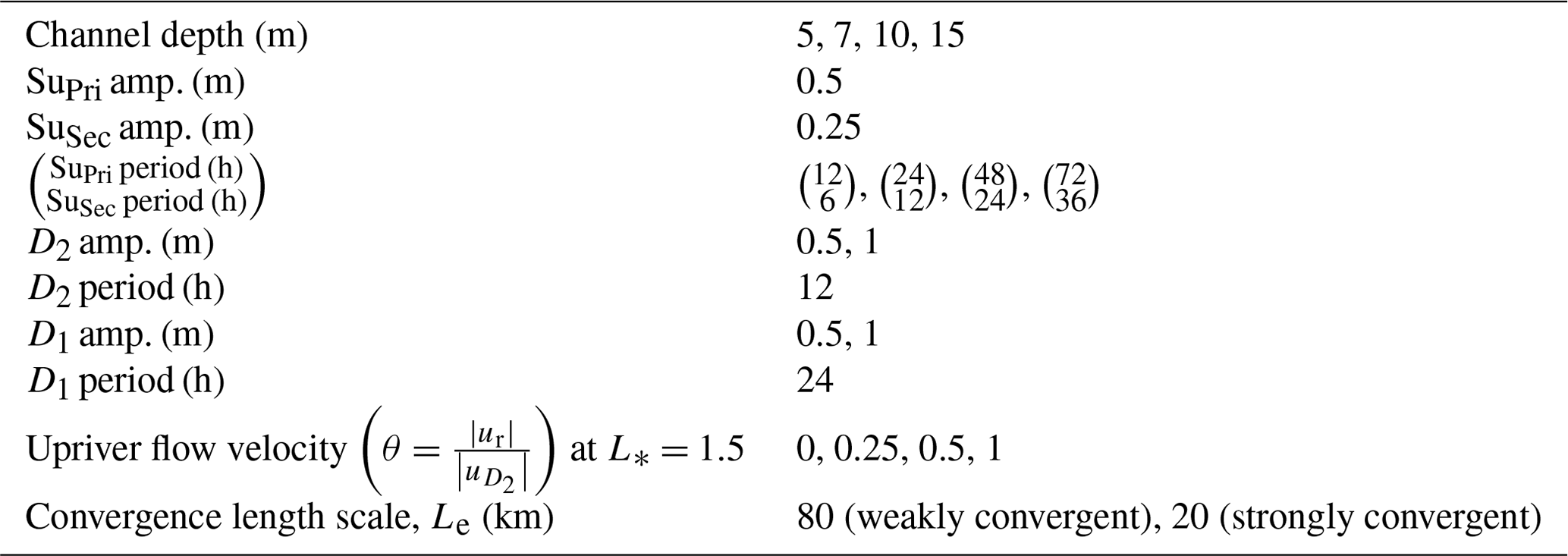
The above tide–surge analytical model has previously been compared against two one-constituent analytical models (the Toffolon and Savenije, 2011, and Jay, 1991, tidal solutions) and idealized Delft-3D numerical model results for situations without river flow (Familkhalili et al., 2020). Results showed that our analytical model is capable of capturing tidal wave amplitudes that are in good agreement with numerical model results. In this section, we update the validation to include the effects of river flow and compare our results against idealized Delft-3D numerical model results using the same bathymetry and forcing (Type I). Following this, we compare our analytical model results against an idealized numerical model developed for the Cape Fear Estuary, North Carolina (Familkhalili and Talke, 2016). This numerical model simulates storm surge from tropical storms by using a parametric model of hurricane wind and pressure forcing that is applied over the continental shelf (Type II). Table 1 shows the model parameters that were used to compare analytical model results with numerical models.

Table 1 Analytical model parameters used in this study. See Appendix A for a description of the parameters. Nondimensional river discharge (θ) is applied at the upstream boundary, and tide and surge waves are applied at the ocean boundary (i.e., the estuary mouth, which is x=0 in Fig. 1).

3.1 Idealized numerical models with similar forcing

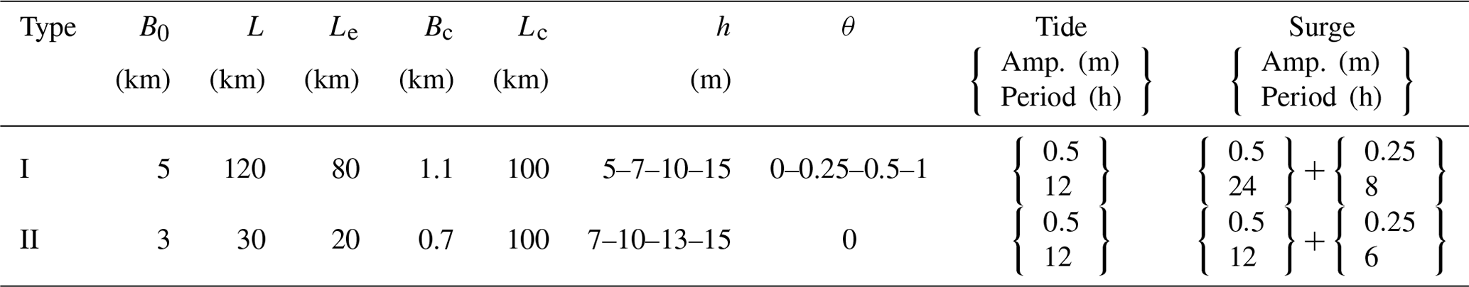
Analytical/numerical comparisons were made for a weakly convergent and strongly dissipative estuary with constant depth of 5m and a width profile defined by Type I (Table 1, see Fig. 1). The estuary section of the model domain (L) is 120 km, 1.5 times the convergence length. Both analytical and numerical models are forced by the K₁, M₂, and M₃ tidal constituents at the ocean boundary, two of which (K₁ and M₃) represent a surge wave when combined (Table 1). We further analyze the numerical model results by using harmonic analysis (e.g., Leffler and Jay, 2009).

Figure 3 shows the spatial pattern of the dominant tidal constituent (M₂) amplitude normalized by its value at the estuary mouth. The analytical model results closely resemble the numerical model results with a root-mean-square error of 0.02 m for the three-wave model with and without river flow (blue and red colors in Fig. 3), showing that this idealized analytical model can properly estimate spatial variability of surge along an estuary.

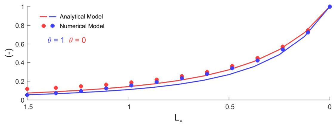
Figure 3 Dominant tidal constituent (M₂) amplitude in a 5 m deep estuary for three tide models (K₁, M₂, and M₃) with and without river flow (θ=0–1). The x axis is the estuary length normalized by the convergence length scale ($L_{\ast }=x/L_{\mathrm{e}}$), and the y axis is normalized by M₂ amplitude at the ocean boundary ($L_{\ast }=\mathrm{0}$).

In addition, results for the tidally averaged water levels (i.e., Z; see Fig. 1) under conditions with both tidal and river flow forcing are consistent with numerical models, as shown in Fig. 4 for a weakly convergent estuary. The water level profiles vary with θ (normalized flow velocity) for both the analytical model (dashed lines) and the numerical model (solid lines). In general, the analytical model slightly underestimates numerical results. The root-mean-square deviation between the numerical and analytical surface profiles are 0.03, 0.08, 0.09, and 0.10 m for a θ of 0, 0.25, 0.5, and 1.0, respectively, or roughly 3 %–8 % of the total super-elevation above sea-level (Fig. 4a). The pattern seen in Fig. 4 can be explained by Eq. (8), in which as river discharge increases (greater θ), the depth-averaged velocity increases, and a larger water surface slope ($\frac{\partial \stackrel{\mathrm{‾}}{H}}{\partial x}$) is needed to balance the Eq. (8).

Figure 4 (a) The importance of river flow (i.e., θ at $L_{\ast }=\mathrm{1.5}$) for 5 m depth and (b) the importance of channel depth for θ=1 in an idealized three-wave model. The vertical axis is tidally averaged water level and horizontal axis represents dimensionless coordinate system of $L_{\ast }=x/L_{\mathrm{e}}$. Solid and dashed lines represent numerical and analytical model results, respectively. The solid and dashed black lines represent the same scenario (h=5 m, θ=1) in both (a) and (b).

3.2 Idealized numerical model with parametric hurricane forcing

We further validate our analytical model results (Type II) with the idealized numerical modeling of Familkhalili and Talke (2016). This model includes a storm surge produced at the continental shelf and six semidiurnal and diurnal tidal constituents. Upstream of river kilometer 12, the estuary is convergent with an e-folding length scale of ∼ 20 km. The analytical model uses similar geometry (Table 1), uses the dominant tidal constituent (M₂) at the estuary mouth, and assumes that the primary surge wave has a period of 12 h. As in the numerical model, river flow is set to zero (Table 1). We compare our analytical results at ∼ $L_{\ast }=\mathrm{1.5}$ with the corresponding location in the numerical model (Wilmington, North Carolina). For a shallow estuary of 7 m, the analytical model suggests that the storm surge wave is damped by ∼ 40 % (from 0.5 to 0.3 m) between the coast and $L_{\ast }=\mathrm{1.5}$ (Fig. 5). This damping is within the range of modeled results for a tropical storm surge at Wilmington (L_∗ ∼ 1.5, Fig. 5). In a deeper configuration (mean depth = 15 m), the analytical model (this paper) finds a 12 % increase in surge amplitude from the coast, well within the normalized amplitude of 0.55–1.35 found in Familkhalili and Talke (2016). Hence, both the sense of change as depth increases and the order of magnitude of change are consistent between the numerical and analytical model, improving our confidence in results (Fig. 5).

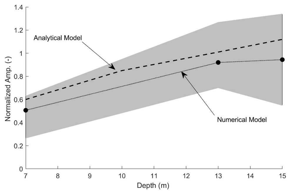
Figure 5 Comparison of normalized surge amplitude as a function of depth for an estuary resembling the Cape Fear Estuary at an inland location at the approximate location of Wilmington, North Carolina. The dashed line is the analytical model result, and the solid line is the numerical result. The idealized numerical model uses a surge event with a mean amplitude of 0.6 m at the ocean boundary (data from Familkhalili and Talke, 2016). The fill area is the range of results due to different relative phase of the storm surge and tide wave. The “analytical model” results are for a 12 h surge that had an amplitude of 0.5 m and is evaluated at $L_{\ast }=\mathrm{1.5}$, i.e., at approximately same location as the numerical model. The y axis is normalized surge amplitude and equals 1 at the ocean boundary.

The results of the model comparison (Figs. 3, 4 and 5) show that both the analytical and idealized numerical models produce broadly consistent results. Therefore, our neglect of acceleration in the subtidal model (Fig. 4) and the use of linearized friction is justified. Both numerical and analytical models are complementary tools. A 3D model with resolved bathymetry is clearly best used to evaluate the specific effect of bathymetric alterations in a particular estuary (e.g., Pareja-Roman et al., 2020; Helaire et al., 2019) or to run simulations using complex, real valued boundary forcing (river and coastal). However, our analytical model runs substantially more quickly than even the idealized numerical models, facilitating investigation of a larger parameter space. Moreover, numerical models cannot unambiguously separate tide, fluvial, and surge effects. Currently, the best-practice approach is to run the numerical model with and without relevant forcing; for example, by running a surge model with and without tides, one can approximate the effect that tides have on total water level (Shen et al., 2006). When combined, tide and surge waves travel faster (due to deeper water depth; see Horsburgh and Wilson, 2007), and frictional energy loss in each wave component is also larger (Familkhalili et al., 2020). Due to the multiple feedbacks and nonlinear interactions, decomposing numerical results into individual surge and tide wave transformations is inherently ambiguous. The analytical approach, while not including all interactions (such as the phase modulation caused by depth variability), is also able to individually estimate transformations in the primary surge and tide constituent amplitudes under different river discharge conditions. This approach, to our knowledge, has not previously been approached to understanding the fundamental bathymetric and boundary condition factors that influence compound events.

3.3 Dimensional and nondimensional parameter space studied

We use our validated analytical model to further investigate the effects of channel depth, river flow, channel width convergence, and surge timescale on the spatial evolution of water levels along estuaries. For all simulations, the primary tidal constituent period and amplitude are fixed to 12 h (i.e., a semidiurnal or D₂ wave) and 0.5 m, respectively, a value that is typical of the semi-diurnal tide wave on the US East Coast (Table 2). To study the effects of width convergence, we test both weakly (L_e=80 km) and strongly convergent (L_e=20 km) conditions (see, e.g., Jay, 1991; Lanzoni and Seminara, 1998). Table 2 shows the parameter space used in the model. The primary and secondary surge amplitudes are set to be 0.5 and 0.25 m, respectively (Eq. 6), and the estuary mouth (B₀) is assumed to have a width of 5 km. A sensitivity analysis is carried out by varying the parameters in Table 2 individually, while other parameters are held constant, resulting in a total of 128 parameter combinations (i.e., four different values for depths, four different values for river flow, four different period combinations, and two convergence length scales).

Table 2 Parameter space used in analytical model.

Nondimensional variables provide insights into which parameters produce the greatest effect on system response. From the scaling of Eq. (3) (see also Familkhalili et al., 2020), we derive the three most relevant independent nondimensional variables.

• Parameter (Ω) represents the ratio of Su_Pri period to D₂ period and represents the influence of primary surge wave period on tide–surge interactions.

• The friction number $\left(\mathit{\psi }=\frac{C_{\mathrm{d}}\mathit{\xi }{\mathit{\omega }}^{\mathrm{2}}{L}_{\mathrm{e}}^{\mathrm{3}}}{g{h}^{\mathrm{3}}}\right)$ shows the effects of changing surge wave properties, which are influenced by depth (h), surge frequency ($\mathit{\omega }=\frac{\mathrm{1}}{T}$), and convergence length scale (L_e), all of which affect the damping or amplification of surge waves.

• Parameter (θ) represents the ratio of upriver velocity (at $L_{\ast }=\mathrm{1.5}$) to the major tidal component (D₂) velocity at the estuary mouth.

For plotting purposes, we define two additional nondimensional numbers: Su_Pri normalized amplitude $\left(A_{\ast }=\frac{{\mathrm{Su}}_{\mathrm{Pri}}\mathrm{amp}.}{\text{surge amp. at ocean boundary}}\right)$ and a dimensionless coordinate system of $L_{\ast }=x/L_{\mathrm{e}}$, where L_∗ is normalized length.

In our models, we assume that the two surge waves are symmetric with a phase lag (ϕ in Eq. 5) of zero degrees between Su_Pri and Su_Sec, resulting in a repeating and symmetric storm surge wave (see Fig. 6). This simulates a storm surge in which there is initially a drawdown in water level, followed by the positive storm surge. To test the most frictional case, we also define the relative phase lag between the D₂ wave and surge to be zero.

Figure 6 A symmetric surge wave that is the result of two sinusoidal waves (i.e., surge $={\mathrm{Su}}_{\mathrm{Pri}}+{\mathrm{Su}}_{\mathrm{Sec}}$).

4 Results and discussion

We employ the validated model to study how bathymetry, river discharge, and surge characteristics affect water floods in an idealized estuary. First, the effects of surge amplitude and period on water levels are examined. Following this, the effects of river discharge and width convergence on surge amplitude are presented, and finally compound flooding of tide, surge, and river flow is investigated.

4.1 Effects of wave characteristics on water level

The influence of wave characteristics (i.e., period and magnitude) on tidally averaged water level is tested by modeling a set of waves with periods of 12 and 24 h and amplitudes of 0.5 and 1 m at the ocean boundary (i.e., D₁ and D₂ in Table 2). Model results confirm, as suggested by the friction number (ψ), that increasing the wave period ($T=\frac{\mathrm{1}}{\mathit{\omega }}$) or decreasing the wave amplitude (ζ) have a similar effect as increasing depth (h), and therefore this would result in lower mean water levels (Fig. 7). Specifically, increasing the wave period from 12 h (red lines) to 24 h (blue lines) reduces the mean water level at $L_{\ast }=\mathrm{1.5}$ from 0.75 to 0.5 m and from 1.56 to 1.10 m for wave amplitudes of 0.5 and 1 m at the ocean boundary ($L_{\ast }=\mathrm{0}$), respectively. In other words, for the same boundary amplitude, a shorter period wave produces larger mean water levels landward.

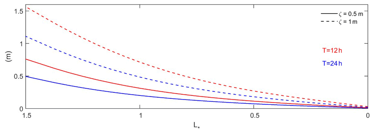
Figure 7 The effects of wave period (i.e., 12 and 24 h) and amplitude (0.5 and 1 m at the ocean boundary $L_{\ast }=\mathrm{0}$) on tidally averaged water level for 5 m depth channel in an idealized one-sinusoidal-wave model for θ=1. The vertical axis is the tidally averaged water level, and the horizontal axis represents the estuary length normalized by the convergence length scale (i.e., $L_{\ast }=x/L_{\mathrm{e}}$).

Figure 8 The effects of river flow $\left(\mathit{\theta }=\frac{\left|u_{\mathrm{r}}\right|}{\left|u_{D_{\mathrm{2}}}\right|}\right)$ and surge periods $\left(\mathrm{\Omega }=\frac{{\mathrm{Su}}_{\mathrm{Pri}}\mathrm{Period}}{D_{\mathrm{2}}\mathrm{Period}}\right)$ along an idealized weakly convergent estuary for channel depth of (a) 5, (b) 7, (c) 10, and (d) 15 m. The color scaling represents the e-folding length scale of the primary surge-normalized amplitude (A_∗).

4.2 Frictional effects of river discharge on surge amplitude

The rate at which a surge decays away from the ocean entrance varies with river flow and surge period. Figure 8 shows the effects of river discharge and surge period on the e-folding length scale of Su_Pri normalized amplitude (A_∗); the e-folding length is distance required for A_∗ to reach $\mathrm{1}/e\sim$ 38 % of boundary values. The longer the wave period, the more slowly the surge-normalized amplitude A_∗ decreases as the surge moves landward (keeping all other variables constant). For example, Fig. 8a shows that a 12 h (Ω=1) surge amplitude reaches an e-folding reduction in amplitude at ∼ 0.4 L_∗ compared to ∼ 0.9 L_∗ for the 72 h (Ω=6) surge. The lower rate of spatial decay of surge amplitude for lower frequency surge waves is caused by their lower velocity and consequent smaller frictional effects.

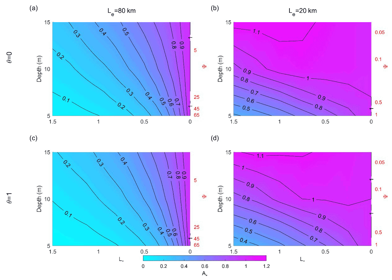
Figure 9 The effects of convergence length scale and river discharge on primary surge (12 h, Ω=1) amplitude (A_∗ is normalized amplitude) along a weakly convergent estuary, L_e=80 km (subplots a, c) and strongly convergent estuary, L_e=20 km (subplots b, d). The left-hand vertical axis is channel depth, the right-hand vertical axis is the corresponding nondimensional friction number $\left(\mathit{\psi }=\frac{C_{\mathrm{d}}\mathit{\xi }{\mathit{\omega }}^{\mathrm{2}}{L}_{\mathrm{e}}^{\mathrm{3}}}{g{h}^{\mathrm{3}}}\right)$, and the horizontal axis represents the dimensionless coordinate system of $L_{\ast }=x/L_{\mathrm{e}}$.

Model results also show that higher river discharge will increase the damping of surge amplitudes (Fig. 8). When θ=0, river flow is zero and only nonlinear tide–surge interactions can occur. Hence, surge amplitudes decay more slowly for θ=0 than for θ>0 (compare the θ=0 and θ=1 cases in Fig. 8). The slanted contour lines highlight the effects of river flow; as θ increases, the e-folding length scale of normalized amplitude (A_∗) reduces for all surge periods (Ω=1–6) (Fig. 8a–d). Adding river flow to a surge with a primary period of 12 h (Ω=1) reduces the e-folding scale of damping from 0.4 L_∗ (θ=0) to 0.34 L_∗ (θ=1) for the 5 m depth case (∼ 15 % decrease; Fig. 8a). The percent decrease in the e-folding scale is larger in a deeper, 15 m channel and decreases from 1.15 to 0.95 L_∗ (∼ 18 % decrease; Fig. 8d).

Surge amplitudes also decay more slowly (larger e folding) in a deeper channel for all surge periods (Fig. 8). Thus, the largest difference in normalized amplitude between a 12 h (Ω=1) and 72 h (Ω=6) surge occurs at larger depth (h=15 m) with changes of ∼ 1 to 3.5 L_∗ in the e-folding length-scale of damping (Fig. 8d). Increasing the river discharge relative to the M₂ velocity (larger θ) reduces the amplification of the surge wave, and therefore the e-folding length scale of A_∗ reduces from ∼ 3.5 to ∼ 2.4 L_∗ for Su_Pri of 72 h (Fig. 8d).

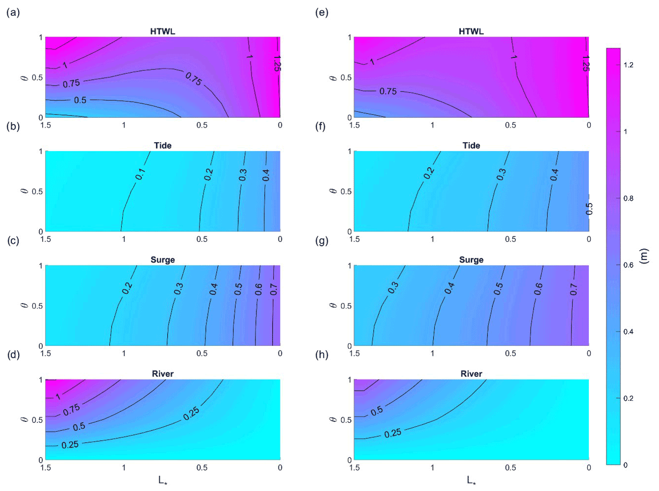
Figure 10 Combined contribution of tide, surge, and river flow to water level for depths of 5 m (left panel subplots) and 10 m (right panel subplots). Colors and the labeled contours denote water level. The total water level (a, e) is the combination of tidal amplitude (b, f), surge amplitude (c, g), and water level from river discharge (d, h). The period of the primary surge (Su_Pri) is 24 h, the convergence length scale is 80 km, the x axis represents the dimensionless coordinate system of $L_{\ast }=x/L_{\mathrm{e}}$ (origin at estuary mouth, on the right-hand side), and the y axis shows the nondimensional river flow $\left(\mathit{\theta }=\frac{\left|u_{\mathrm{r}}\right|}{\left|u_{D_{\mathrm{2}}}\right|}\right)$.

Consistent with other studies (e.g., Kukulka and Jay, 2003b; Hoitink and Jay, 2016), both the analytically and numerically modeled water level slope ($\mathrm{d}Z/\mathrm{d}{L}_{\ast }$) are largest upstream and become significantly smaller near the coast. This is caused by the decreased river velocity (and friction) associated with the downstream increase in cross-sectional area. Therefore, we expect that varying the forcing or the geometry will impact mean water levels upstream, as river velocity magnitudes shift.

4.3 Effects of width convergence on surge amplitude

Long-wave propagation along an estuary is characterized by a balance of inertial effects, friction, and convergence. Figure 9 shows the normalized amplitude (A_∗) of the primary surge wave for weakly convergent (left panel, 9a and c) and strongly convergent estuaries (right panel, 9b and d), for a 12 h surge period (Ω=1). The contours represent the e-folding length scale of primary surge-normalized amplitude and the x axis represents the dimensionless coordinate system of $L_{\ast }=x/L_{\mathrm{e}}$. The factor of 4 change in convergence length scale from 80 (Fig. 9a, c) to 20 km (Fig. 9b, d) alters the friction scale (ψ) by a factor of 64.

The convergence of an estuary influences surge amplitudes (Fig. 9), similar to its well-known effects on tidal amplitudes (e.g., Jay, 1991). All surge amplitudes decrease landward for all depth cases in a weakly convergent (L_e=80 km) estuary; effectively, convergence effects are much smaller than the bed friction and gravity effects, and therefore long wave amplitudes decrease (Fig. 9a and c). Under strongly convergent conditions with no river flow, the primary surge amplitude decays less quickly in a deeper channel as it moves upstream than under weakly convergent condition (see Fig. 9a, b) and can even increase in the inland direction (see Fig. 9b). By contrast, increased river discharge produces greater damping in the surge wave (compare Fig. 9a and c, or Fig. 9b and d). For example, for friction factor of ψ=0.5 (h=6.5 m) and a location of $L_{\ast }=\mathrm{1}$, the surge wave has damped to 60 % of its boundary value when the tidal to river flow ratio is θ=1 (Fig. 9d) but is at 70 % of its boundary value when there is no river discharge (Fig. 9b). Hence, increasing river flow and decreasing channel depth both cause larger damping in the surge wave.

4.4 Combined effects of tide, surge, and river flow on total water levels

We next investigate how variations in river flow influence the total water level (TWL), caused by the combination of tide, storm surge, and river discharge effects. The highest possible total water level (HTWL) during such a compound event occurs when the surge occurs at high water, coincident with peak river flow. Because the timing of a meteorological event is usually random relative to tides, and because peak surge usually precedes peak river discharge, HTWL rarely if ever occurs. However, it is a useful metric of the potential flooding. Such a worst-case scenario could occur, for example, when multiple storms occur in close succession. The HTWL therefore provides a way to compare different parameter regimes and evaluate the effect of long-term changes in the geometry of an individual estuary.

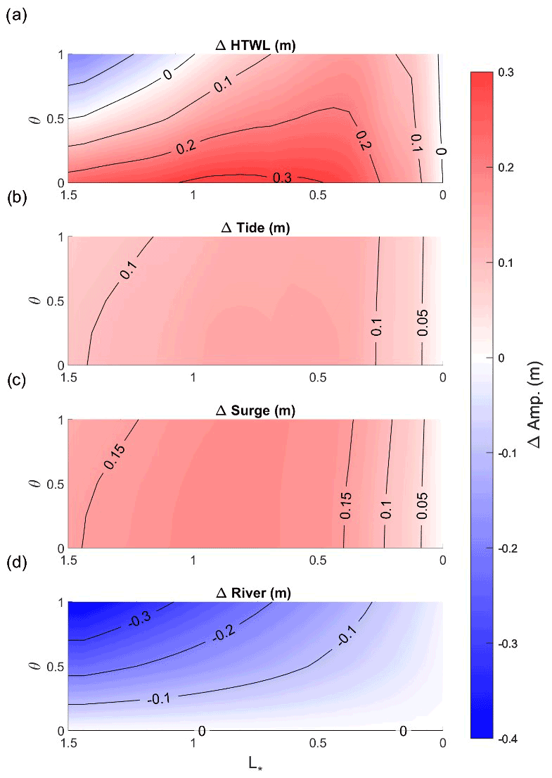
Figure 11 Comparison of the contribution of tide, surge, and river flow to compound flooding between 5 and 10 m depth channel and Su_Pri=24 h. Δ represents the amplitude difference of each factor (HTWL, tide, surge, and river flow) between two controlling depths. The convergence length scale is 80 km, the x axis represents the dimensionless coordinate system of $L_{\ast }=x/L_{\mathrm{e}}$, and the y axis shows nondimensional river flow $\left(\mathit{\theta }=\frac{\left|u_{\mathrm{r}}\right|}{\left|u_{D_{\mathrm{2}}}\right|}\right)$.

The HTWL (Fig. 10a and e) follows a pattern set by the contradictory effects of river flow and marine forcing (tides and surge). Far upstream ($L_{\ast }=\mathrm{1.5}$), river water levels are the largest factor, particularly for larger θ, but decay in the downstream direction (Fig. 10d, h). The surge and tidal components of water level (e.g., Fig. 10b, c) decay in the opposite direction, from the oceanic boundary towards the upstream boundary. For larger river flows (∼ θ > 0.5), the counteracting factors produce a minimum HTWL in the middle part of the domain ($L_{\ast }=\mathrm{0.5}$–1.0). For small river flows, water levels monotonically decrease in the upstream direction.

Importantly, the HTWL is not merely the superposition of river flow, tide, and surge effects considered in isolation. Rather, as shown by the non-vertical contour lines for tides and surge (e.g., Fig. 10f and g), increases in the relative influence of river flow (larger θ) tend to reduce the magnitude of tides and surge (see also Helaire et al., 2020). By contrast, increases in long wave magnitudes (tides, surge) at the ocean boundary increase the tidally averaged water level profile, as already established (Fig. 7; see also Buschman et al., 2009; Talke et al., 2021). Simultaneously, long wave magnitudes decrease more quickly the larger they are at the ocean boundary (see also Familkhalili et al., 2020). Effectively, each component of water level influences the other as well as itself: for example, tides within the domain depend on self-interaction (e.g., the boundary magnitude matters) and also on tide–surge and tide–river interaction. While the overall influence in terms of magnitude is relatively minor for the parameter space in Fig. 10, these observations show that nonlinear tide–surge–river interactions during a compound event cannot be neglected. In particular, interactions would be larger in macrotidal systems and/or for larger surges.

Figure 12 Crossover point location for 7–15 m channel depth compared to the 5 m case, (Su_Pri=24 h and L_e=80 km). The x axis represents the dimensionless coordinate system of $L_{\ast }=x/L_{\mathrm{e}}$, and the y axis shows nondimensional river flow $\left(\mathit{\theta }=\frac{\left|u_{\mathrm{r}}\right|}{\left|u_{D_{\mathrm{2}}}\right|}\right)$.

Changes in the depth of an estuary, whether by dredging, sea-level rise, or sedimentation and erosion, also exert a strong, spatially variable influence on the HTWL (Figs. 10 and 11). When depth is small (5 m; Fig. 10a), the HTWL is greater in the upstream domain ($L_{\ast }=\mathrm{1.5}$ and θ>0.5) than in a larger depth case (10 m; Fig. 10e). This occurs because a larger average river slope is needed to push the same amount of water seaward when the depth is small, as suggested by Eq. (8) (see also Talke et al., 2021). However, smaller depths also lead to greater dissipation and frictional effects in the tide and surge wave due to the same reduction in hydraulic drag (compare the right-hand and left-hand sides of Fig. 10 and their differences, as well as Fig. 11). Hence, tide and surge amplitudes increase when depth increases for all river discharges (θ=0–1; Fig. 11b, c). The percent increase is less for higher river discharge; this is evident from the rightward slant of contours in Fig. 11b and 11c. Further, both tides and surge show a region of maximum change, located mid-estuary (between $L_{\ast }=\mathrm{0.5}$ to 1; Fig. 11). Near the ocean boundary, changes are also relatively small in percentage terms. Far upstream, the percent change in tidal range may still be significant, but the magnitudes themselves are small (see also Talke et al., 2021).

The differences in the response of river flow and storm surge to a depth increase lead to a crossover point, which we define as the location in which river flow effects on HTWL are larger than marine effects for a given set of forcing conditions (see the zero-contour line in Fig. 11a). Since the crossover point moves upstream as depth increases (Fig. 12), processes such as dredging, erosion, or sea-level rise that increase depth can alter the relative influence of marine and river effects, for a given storm surge and river flow. Similarly, a decrease in mean river inflow, as has occurred in many river estuaries due to flow regulation, may also cause a landward migration in the crossover point (Fig. 12).

Other factors that influence long wave amplitudes also influence the crossover point, including the period of the surge (Fig. 8), convergence length L_e (Fig. 9), boundary amplitude, and relative phasing of tides and surge (see Familkhalili et al., 2020). The influence of many of these factors is explained by considering the nondimensional friction number $\left(\mathit{\psi }=\frac{C_{\mathrm{d}}\mathit{\xi }{\mathit{\omega }}^{\mathrm{2}}{L}_{\mathrm{e}}^{\mathrm{3}}}{g{h}^{\mathrm{3}}}\right)$ (see Sect. 2.1). This number suggests that increases in channel depth (h) and wave period ($T=\frac{\mathrm{1}}{\mathit{\omega }}$) and decreases in length scale (L_e) have similar effects on wave amplitudes. For example, increasing the depth from 5 m (ψ=69) to 15 m (ψ=2.6) causes A_∗ (i.e., normalized amplitude by ocean boundary amplitude) to increase from ∼ 0.06 to 0.26 (Fig. 9a). Similarly, changing the surge period from 12 to 60 h (ψ=69 to 2.8) changes A_∗ from ∼ 0.06 to 0.22 for a 5 m channel depth.

Other studies, such as Bilskie and Hagen (2018), have defined flood zone transitions between marine and fluvial dominance; close to the coast, tide and surge-based flooding dominates, while river floods dominate far upstream. In between, there is a transition zone with compound flooding in which both coastal and fluvial processes are important. Here, our model also suggests that the transition zone location is sensitive to changes in estuary geometry, such as depth, in addition to being dependent on the relative strength of river flow, tide, and surge amplitudes.

5 Conclusions

In this study, we have applied a new river–tide–surge analytical model to investigate the interactions of tide, surge, and river flow along idealized estuaries. The novelty of our approach is that we develop a quasi-linear analytical model, previously applied to tides, that considers the nonlinear interaction between tides, storm surge, and river discharge. To the best of our knowledge, these processes (river flow + surge + tides) have not been explored within an analytical framework. The model also elucidates the trade-offs caused by channel deepening, which can reduce mean water levels but increase storm surge and tides.

We show that the rate of damping in a storm tide (surge + tide) is sensitive to fluctuations of river discharge (Fig. 8), alterations in the surge period (Fig. 8), and channel geometry changes (width convergence and depth) (Fig. 9). Model results show that the crossover point, which is the location at which the river flow effects are larger than marine effects, moves upstream as channel depth increases or as river flow decreases (Fig. 12). Thus, the spatial variability in compound flood risk contributors (i.e., tide, surge, and river flow) change when an estuary is modified or river discharge changes. Generally, increasing the surge period has a similar effect as increasing the depth; however, we note that our model is slightly more sensitive to depth, which is due to the cubic relationship in the friction term rather than the squared effect of period. The nondimensional friction number (ψ) suggests that the effects of surge amplitude at boundary (ξ) and drag coefficient (C_d) have a lesser, but still important, influence on the spatial damping of surge as the depth. We conclude that in a shallow estuary the effects of friction are dominant over the convergence and cause the wave amplitudes (tides and surge) to decrease, while deepening the estuary may cause amplification of long waves upriver of an estuary. As shown in Fig. 9, the amplification in storm surge is particularly acute when the estuary is highly convergent.

Globally, natural and local anthropogenic changes in estuaries (e.g., sea-level rise, channel deepening for navigation and landfilling) produce alterations in tidal and surge amplitudes (see review by Talke and Jay, 2020, and references therein). This study shows that river flow and its interaction with tides and surge must also be considered when evaluating changes to water levels. For example, increasing the river discharge relative to tide velocity reduces the amplification of the surge wave. Moreover, channel deepening produces a reduction in the water level caused by river discharge, leading to a domain in which channel deepening produces lower water levels upstream but larger water levels in the estuary (Figs. 10–12; see also Helaire et al., 2019; Ralston et al., 2019). Our findings are consistent with other studies that find that reduced frictional effects (e.g., caused by channel deepening) can cause increases to tides and surge (see, e.g., Ralston et al., 2019; Talke et al., 2021). Overall, anthropogenic changes to estuary geometry and frictional characteristics can cause large changes in the amplitude and spatial distribution of compound flooding.

Appendix A

This glossary provides definitions of the terms used in this paper.

Name	Definition	Unit
A	Channel cross-sectional area	m2
A∗	Ratio of primary surge amplitude within the estuary to the surge wave amplitude at ocean boundary	–
b	Channel width	m
B0	Estuary mouth width	m
Bc	River width	m
Cd	Drag coefficient	–
D1	Diurnal tidal constituent	–
D2	Semidiurnal tidal constituent	–
g	Gravitational acceleration	m s−2
h	Channel depth	m
K	Bed stress divided by water density	m2 s−2
L	Length of estuary	m
Le	Convergence length scale of estuary width	m
Lc	Constant width river channel length	m
L∗	Normalized length	–
Q	Cross-sectionally integrated flow	m3 s−1
QR	River flow discharge	m3 s−1
QT	Tidal transport	m3 s−1
SuPri	Primary surge wave	–
SuSec	Secondary surge wave	–
t	Time	s
T	Surge period	s
uR	River flow velocity	ms−1
uT	Tidal velocity	ms−1
UR	Maximum river flow velocity	ms−1
UT	Maximum tidal velocity	ms−1
x	Along channel distance (estuary mouth is at x= 0 and x increases landward)	m
ξ	Tidal amplitude	m
θ	River velocity magnitude to the magnitude of the major tidal component velocity at the ocean boundary	–
ρ	Water density	kg m−3
ϕ	Wave phase	rad
ω	Wave frequency	s−1
Ω	Ratio of primary surge period to main tidal component period	–
ψ	Friction number	–