the Creative Commons Attribution 4.0 License.
the Creative Commons Attribution 4.0 License.
 | 01 Aug 2022
The role of wind, mesoscale dynamics, and coastal circulation in the interannual variability of the South Vietnam Upwelling, South China Sea – answers from a high-resolution ocean model
Thai To Duy
Claude Estournel
Patrick Marsaleix
Thomas Duhaut
Long Bui Hong
Ngoc Trinh Bich
The South Vietnam Upwelling (SVU) develops in the South China Sea (SCS) under the influence of southwest monsoon winds. To study the role of small spatiotemporal scales on the SVU functioning and variability, a simulation was performed over 2009–2018 with a high-resolution configuration (1 km at the coast) of the SYMPHONIE model implemented over the western region of the SCS. Its capability to represent ocean dynamics and water masses from daily to interannual scales and from coastal to regional areas is quantitatively demonstrated by comparison with available satellite data and four in situ datasets. The SVU interannual variability is examined for the three development areas already known: the southern (SCU) and northern (NCU) coastal upwelling areas and the offshore upwelling area (OFU). Our high-resolution model, together with in situ observations and high-resolution satellite data, moreover shows for the first time that upwelling develops over the Sunda Shelf off the Mekong Delta (MKU).
Our results confirm for the SCU and OFU and show for the MKU the role of the mean summer intensity of wind and cyclonic circulation over the offshore area in driving the interannual variability of the upwelling intensity. They further reveal that other factors contribute to SCU and OFU variability. First, the intraseasonal wind chronology strengthens (in the case of regular wind peaks occurring throughout the summer for SCU or of stronger winds in July–August for OFU) or weakens (in the case of intermittent wind peaks for SCU) the summer average upwelling intensity. Second, the mesoscale circulation influences this intensity (multiple dipole eddies and associated eastward jets developing along the coast enhance the SCU intensity). The NCU interannual variability is less driven by the regional-scale wind (with weaker monsoon favoring stronger NCU) and more by the mesoscale circulation in the NCU area: the NCU is prevented (favored) when alongshore (offshore) currents prevail.
- Article
(20267 KB) - Full-text XML
-
Supplement
(516 KB) - BibTeX
- EndNote


Ocean circulation in the South China Sea (SCS), one of the largest semi-enclosed seas in the world (Fig. 1), is under the influence of several factors of variability at different scales: typhoons, seasonal monsoon, interannual to decadal variability, and climate change (Wyrtki, 1961; Herrmann et al., 2020, 2021). The SCS is moreover impacted by human activities, with highly densely populated coastal areas (Center for International Earth Science Information Network – CIESIN – Columbia University, 2018), which generate problems such as marine pollution (release of industrial, agricultural or domestic contaminants, such as pharmaceuticals, pesticides, heavy metals, or plastics). Reciprocally, coastal societies are highly dependent on marine resources (fisheries and aquaculture, tourism, etc.). The SCS also influences the functioning and variability of regional climate through air–sea coupling (Xie et al., 2003, 2007; Zheng et al., 2016). It also influences global climate through its role in the transformation of surface water masses of the global ocean circulation (South China Sea Throughflow, Fang et al., 2009; Qu et al., 2009). It is therefore essential to better understand and model SCS's different scale dynamics which intervene in the transport and fate of water masses, in the cycle of water and energy, in the functioning of planktonic ecosystems (via their impact on the transport and mixing of nutrients and organic matter, Ulses et al., 2016; Herrmann et al., 2017), and in the propagation of contaminants at sea.
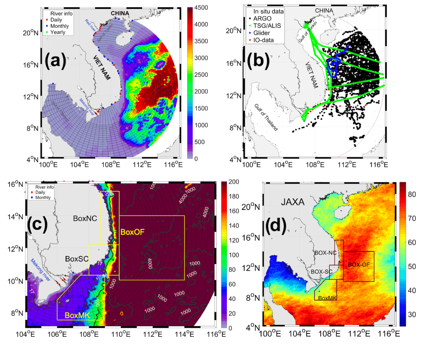
Figure 1(a) Characteristics of the orthogonal curvilinear computational grid (black lines, not all points are shown for visibility purposes) and bathymetry (colors, meter, GEBCO_2014) used for the VNC configuration of the SYMPHONIE model. Dots show the location of rivers for which we used daily (red), monthly (blue) and yearly climatology (green) discharge values. (b) Location of in situ data available over the VNC domain: ARGO buoys (black), the R/V ALIS campaign (TSG: green), IO-18 data (red), and glider data (blue). (c) Bathymetry (m) over the SVU region. Yellow boxes show the location of the four boxes used for the study of SVU. (d) Percentage of days during which JAXA data are available during summer 2018.
The large-scale summer SCS circulation is usually characterized by an overall anticyclonic circulation that results from southwest summer monsoon winds (Wang et al., 2004). It is composed more precisely of a western boundary current and a dipole structure that develops along the Vietnamese coast, with an anticyclonic gyre (AC) in the south and a cyclonic gyre (C) in the north (see Fig. 2l). This dipole structure induces northward and southward alongshore coastal currents which are the western components of the anticyclonic and cyclonic (ACC) gyres and a marked eastward offshore jet that develops in the area of convergence of both coastal currents and between both gyres, around ∼ 12∘ N (Wyrtki, 1961; Fang et al., 2002; Xie et al., 2003, 2007; Chen and Wang, 2014; Li et al., 2014, 2017).
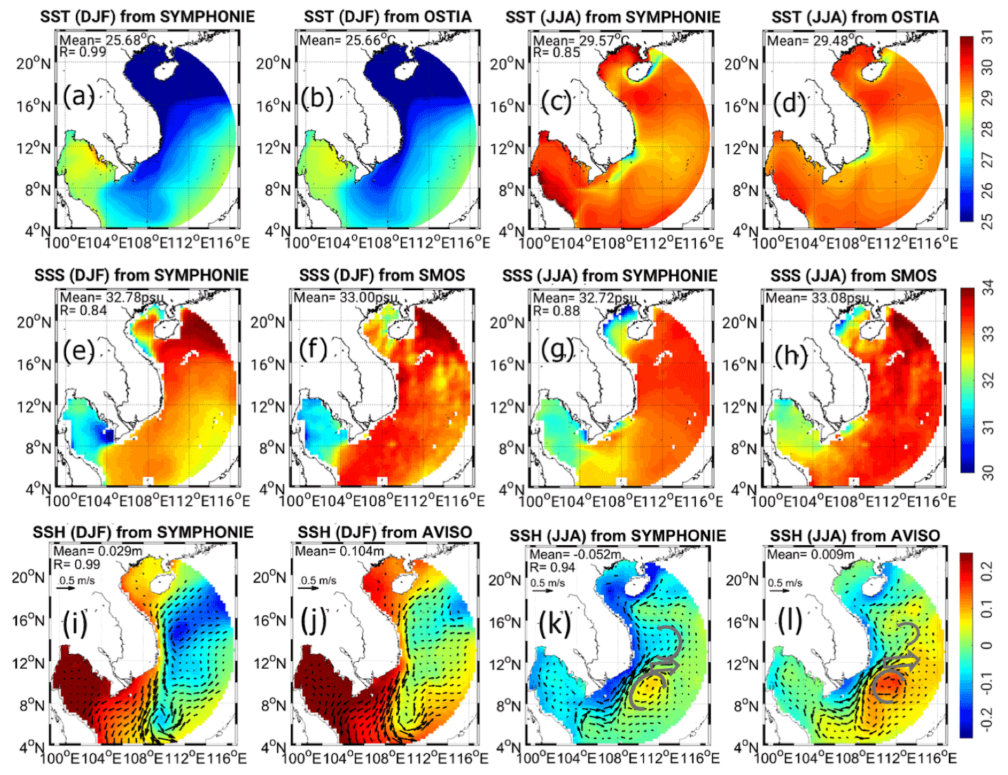
Figure 2Spatial distribution of simulated and observed winter (DJF) and summer (JJA) climatological averages of SST (a, b, c, d, ∘C), SSS (e, f, g, h), SSH (i, j, k, l, m), and total surface geostrophic current (m s−1) and spatial correlation coefficient R (here the p value is always smaller than 0.01). Gray arrows on panels (k)–(l) highlight the summer ACC dipole and eastward jet.
Summer wind forcing and the resulting large-scale circulation (ACC dipole + eastward jet) induce the South Vietnam Upwelling (SVU), one of the main components of the SCS summer ocean dynamics. The SVU strongly influences halieutic resources through its impact on bio-productivity (Bombar et al., 2010; Loick et al., 2007; Loisel et al., 2017; Lu et al., 2018). It also affects regional climate (Xie et al., 2003; Zheng et al., 2016). It is driven at the first order by atmospheric forcing, namely Ekman transport and pumping induced by the southwest monsoon wind (Xie et al., 2003). It is moreover reinforced by the eastward jet that enhances the offshore advection of coastal water (Dippner et al., 2007a) and by the combination of wind-induced Ekman pumping and positive surface current vorticity associated with cyclonic eddies in the offshore area (Da et al., 2019; Ngo and Hsin, 2021). These studies showed that upwelling develops over several areas. The most studied areas are the southern coastal area and the offshore area. The southern coastal upwelling (named SCU hereafter) develops along the Vietnamese coast between 10.5 and 12∘ N in the area of convergence between the northern southward and southern northward boundary currents (Figs. 2l, 3). The offshore upwelling (named OFU hereafter) develops over a large offshore region, in the area of cyclonic circulation north of the eastward jet. Two studies moreover showed that upwelling sometimes develops along the northern part of the Vietnamese coast (named NCU hereafter), from 11 to 15∘ N. Da et al. (2019) revealed from Advanced Very High Resolution Radiometer (AVHRR) SST (sea surface temperature) satellite data and from a ∘ simulation that upwelling developed during summer 1998 in this area, and Ngo and Hsin (2021) studied the interannual variability of the NCU using gridded satellite data.
Previous field campaigns (Dippner et al., 2007a; Bombar et al., 2010; Loick-Wilde et al., 2017), satellite observations (Xie et al., 2003; Kuo et al., 2004; Ngo and Hsin, 2021), and modeling studies (Li et al., 2014; Da et al., 2019) showed that the SVU intensity strongly varies from one year to another. This interannual variability depends in particular on the intensity of the summer monsoon southwest wind and on ENSO (El Niño–Southern Oscillation) but also on cross-equatorial winds (Xian et al., 2019) and decadal climate variability (Wang and Wu, 2020). Previous studies showed that the interannual variability of the SCU is mainly triggered by the interannual variability of the summer-averaged wind stress that induces Ekman transport (Chao et al., 1996; Dippner et al., 2007b; Da et al., 2019; Ngo and Hsin, 2021). Using long simulations or datasets, two recent studies established statistical relationships between the interannual variability of SCU and OFU intensity, the atmospheric forcing, and the ocean circulation. Da et al. (2019) used a ∘ (∼ 9 km) 14-year simulation. Ngo and Hsin (2021) used ∘ (∼ 28 km) datasets of 38-year SST and reanalysis winds and of 28-year satellite-altimeter-derived sea surface currents. Da et al. (2019) simulated an Ekman pumping-related OFU that develops under the influence of strong positive wind curl. They obtained a highly significant correlation between the yearly intensity of upwelling and the summer average of wind stress (0.70, p<0.01) and wind stress curl (0.72, p<0.01) over the region. They showed that SVU intensity is also correlated with the summer average of positive vorticity of surface current over the offshore area (0.79, p<0.01). This vorticity, which quantifies the intensity of the ACC dipole and eastward jet circulation, partly results from the wind forcing, with a 0.73 (p<0.01) and 0.63 (p<0.02) correlation with summer average wind stress and wind stress curl, respectively. Some authors moreover showed that the wind also influences the SVU at the intraseasonal scale, with SVU developing after peaks of strong winds induced by the Madden–Julian Oscillation (MJO) and typhoons (Xie et al., 2007; Liu et al., 2012). Da et al. (2019) moreover revealed and quantified the important contribution of ocean intrinsic variability (OIV) in the SVU interannual variability in the offshore area. They showed that this OIV contribution is related to the role of vorticity associated with mesoscale structures, whose propagation is strongly stochastic: cyclonic (anticyclonic) mesoscale eddies located in the area of positive wind curl enhance (weaken) the summer average intensity of offshore upwelling. Ngo and Hsin (2021) confirmed the relationship between the interannual variability of the summer regional wind stress curl, the induced offshore circulation (i.e., eastward jet, ACC dipole, and associated northward/southward boundary currents), and the SCU and OFU intensity: they showed that upwelling is stronger (weaker) for years of stronger (weaker) wind stress curl and large-scale circulation (eastward jet and dipole). Finally, Chen et al. (2012) showed that tides and river plumes could be additional mechanisms involved in SVU dynamics, using idealized simulations. Tide effect was not included in most modeling studies, including Da et al. (2019).
Most previous studies were therefore based on numerical or observational datasets associated with several methodological choices and hypothesis: short study periods and limited spatial coverage of in situ datasets; model resolution coarser than ∼ 10 km; cloud cover and proximity of the coast hindering satellite data quality; gridded current datasets built from along-track sea level satellite data that cannot capture small-scale and ageostrophic dynamics; synoptic view based on spatially and seasonally integrated atmospheric and oceanic variables; no or simplified representation of tides and river plumes, etc. This limited their capability to capture or represent the full range of scales involved in the SVU variability that goes from submesoscale and coastal dynamics to regional circulation and from daily to interannual variability. In particular, the settings of those modeling and observational studies did not allow them to capture the variations at small spatial scales and high frequency of ocean SST and dynamics, including the effect of tides. To improve our knowledge of SVU functioning and variability, further investigations are therefore needed to better monitor, represent, and understand the behavior of upwelling at smaller spatial (meso- to submesoscales) and temporal (intraseasonal variability) scales and over detailed areas (coastal to offshore). First, this requires understanding how ocean dynamics at those smaller spatial scales, which largely contribute to OIV (Sérazin et al., 2016; Waldman et al., 2018), and their interactions with larger-scale circulation contribute to the SVU functioning and variability. Second, this requires examining how high-frequency variability (daily to intraseasonal) of atmospheric forcing and ocean dynamics, including tides, influences the summer-averaged SVU intensity and its interannual variability. With the goal of better modeling and understanding the functioning and variability of ocean dynamics at small spatial and temporal scales and their influence on the SVU summer intensity and interannual variability, we thus developed a high-resolution configuration of a numerical ocean model, able to represent ocean dynamics and water masses at all scales from the Vietnamese coast to the offshore region.
The model is presented in Sect. 2. Its capability to represent ocean dynamics and water masses is evaluated in Sect. 3. We then used this model to examine the variability of the SVU at different scales. Here we first focus on its interannual variability over its four main areas of development, examining in particular the role of high-frequency and small-scale dynamics. This analysis is presented in Sect. 4. Results are discussed in Sect. 5 and summarized in Sect. 6.
2.1 The regional ocean hydrodynamical model SYMPHONIE
The 3D ocean circulation model SYMPHONIE (Marsaleix et al., 2008, 2019) is based on the Navier–Stokes primitive equations solved on an Arakawa curvilinear C grid under the hydrostatic and Boussinesq approximations. The model makes use of an energy conserving finite difference method described by Marsaleix et al. (2008), a forward–backward time stepping scheme, a Jacobian pressure gradient scheme (Marsaleix et al., 2009), the equation of state of Jackett et al. (2006), and the K–epsilon turbulence scheme with the implementation described in Michaud et al. (2012) and Costa et al. (2017). Horizontal advection and diffusion of tracers are computed using the QUICKEST scheme (Leonard, 1979), and vertical advection is computed using a centered scheme. Horizontal advection and diffusion of momentum are each computed with a fourth-order centered biharmonic scheme as in Damien et al. (2017). The viscosity of momentum associated with this biharmonic scheme is calculated according to a Smagorinsky-like formulation derived from Griffies and Hallberg (2000). The lateral open boundary conditions for temperature, salinity, current, and sea surface height, based on radiation conditions combined with nudging conditions, are described in Marsaleix et al. (2006) and Toublanc et al. (2018). The VQS (vanishing quasi-sigma) vertical coordinate described in Estournel et al. (2021) is used to avoid an excess of vertical levels in very shallow areas while maintaining an accurate description of the bathymetry and reducing the truncation errors associated with the sigma coordinate (Siddorn and Furner, 2013).
The configuration used in this study is based on a standard horizontal polar grid (Estournel et al., 2012) with a resolution decreasing linearly seaward, from 1 km at the Vietnamese coast to 4.5 km offshore (Fig. 1a), and 50 vertical levels. This configuration with a refined resolution on the Vietnam coast is hereafter referred to as the Vietnam coast (VNC) configuration. The simulation runs from 1 January 2009 to 31 December 2018. The atmospheric forcing is computed from the bulk formulae of Large and Yeager (2004) using the 3-hourly output of the European Center for Medium-Range Weather Forecasts (ECMWF) ∘ atmospheric analysis, distributed on http://www.ecmwf.int (last access: 25 July 2022). In particular wind stress τ is computed from ECMWF wind velocity based on the bulk formula of Large and Yeager (2004): , where u10 is the wind velocity at 10 m height, ρa is the air density computed from sea level pressure SLP and air temperature at 2 m T2m, , and Cd is the nonlinear drag coefficient computed from Large and Yeager (2004). The horizontal wind stress curl WS is then computed as the vertical component of the wind stress rotational: , where τx and τy are, respectively, the zonal and meridional components of τ. Initial ocean conditions and lateral ocean boundary conditions are prescribed from the daily outputs of the global ocean ∘ analysis PSY4QV3R1 distributed by the Copernicus Marine and Environment Monitoring Service (CMEMS) on http://marine.copernicus.eu (last access: 25 July 2022). The implementation of tides follows Pairaud et al. (2008, 2010). It includes tidal amplitude and phase introduced at open lateral boundaries and the astronomical plus loading and self-attraction potentials and considers the nine main tidal harmonics, provided by the 2014 release of the finite-element solution (FES) global tidal model (Lyard et al., 2006). As the absence of tides in the 3D COPERNICUS simulation led to an underestimation of T (temperature) and S (salinity) mixing near the bottom, we add to the COPERNICUS fields the tidal mixing effect, using the parameterization described in Nguyen-Duy et al. (2021). The boundary conditions for rivers are described in Reffray et al. (2004) and Nguyen-Duy et al. (2021). Three kinds of river runoff data were available over the VNC region: monthly climatology data for 17 rivers, yearly climatology data for 1 river, and daily real-time data for 18 rivers (see Fig. 1a for locations of river mouths). The total freshwater discharge of the 36 rivers is equal on average over 2009–2018 to 21.4×10³ m3 s−1. To account for the interannual variability of river discharges for climatological data, we applied to those climatological data a yearly multiplying coefficient obtained from daily data time series.
2.2 Observation data
2.2.1 Satellite data
Available satellite observations are used to evaluate the capability of the model to reproduce sea surface characteristics over the study area:
-
OSTIA (Operational Sea Surface Temperature and Sea Ice Analysis) level-4 analysis daily SST produced using an optimal interpolation approach by the Group for High-resolution SST (GHRSST, UKMO, 2005) on a global 0.05∘ grid over the period 2009–present, available at ftp://data.nodc.noaa.gov/pub/data.nodc/ghrsst/L4/GLOB/UKMO/OSTIA/ (last access: 25 July 2022);
-
Boutin et al. (2018) version 3 of 9 d averaged level-3 sea surface salinity (SSS) derived from the Soil Moisture and Ocean Salinity (SMOS) microwave imaging radiometer with aperture synthesis (MIRAS) measurements at 0.25∘ resolution over 2010–2017, available at ftp://ext-catds-cecos-locean:catds2010@ftp.ifremer.fr (last access: 25 July 2022);
-
Daily altimetry sea level (SSH, sea surface height) data produced by AVISO (Archiving, Validation and Interpretation of Satellite Oceanographic data) at a 0.25∘ resolution over the period from 1993 up to now (Ablain et al., 2015; Ray and Zaron, 2016), distributed by the CMEMS on http://marine.copernicus.eu (last access: 25 July 2022);
-
JAXA (Japan Aerospace Exploration Agency) daily SST (Level 3) dataset provided from Himawari Standard Data by JAXA over the period 2015–present with a 2 km spatial resolution – we only consider JAXA data of quality levels ≥ 4.
For model–data comparisons, model outputs are interpolated on spatial and temporal grids of data.
2.2.2 In situ data
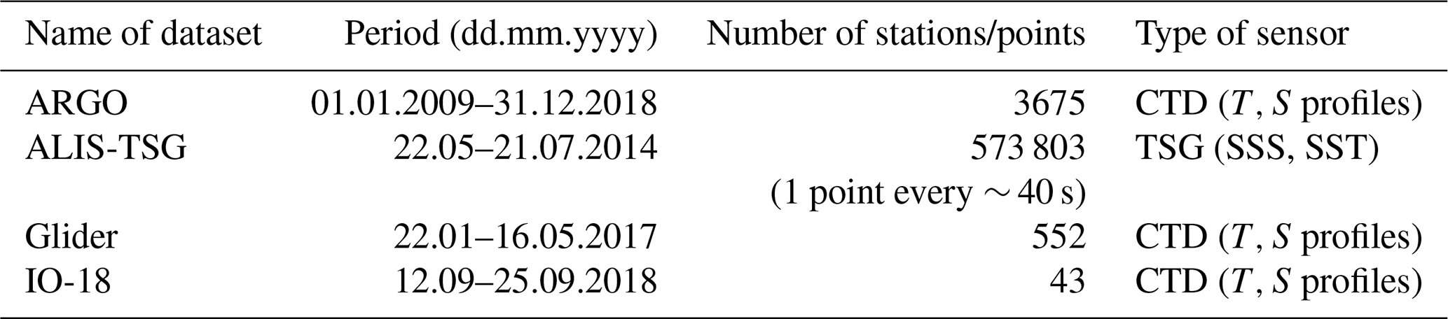
To evaluate the capability of the model to reproduce temperature and salinity (TS) characteristics of water masses, we collected and processed temperature and salinity in situ data available over the study area (see measurement characteristics in Table 1 and locations in Fig. 1b). The modeled outputs were spatially and temporally co-localized with observations used for comparison.
-
ARGO floats. Over the period 2009–2018 more than 3600 TS profiles were collected in the VNC domain. The data are available on ftp://ftp.ifremer.fr/ifremer/argo/geo/pacific_ocean/ (last access: 25 July 2022).
-
Sea-glider Vietnam – United States campaign. Under the framework of a cooperative international research program (Rogowski et al., 2019), a Seaglider sg206 was deployed on 22 January 2017 and crossed the shelf break approximately four times before the steering mechanism malfunctioned on 21 April 2017. The mission ended on 16 May 2017. The glider collected 552 vertical profiles over the 114 d of deployment (hereafter called GLIDER data).
-
R/V ALIS data. The VITEL cruise was organized in May–July 2014 on the French R/V ALIS. During the ALIS trajectory in the SCS, surface temperature and salinity were measured every 6 s, from 10 May to 28 July 2014 by the automatic thermosalinometer (TSG) Seabird SBE21 (hereafter called ALIS-TSG data).
-
IO-18 data. Meteorological, current, temperature, and salinity parameters were measured by the IO (Institute of Oceanography) in the framework of the Vietnamese State project in September 2018. Measurements were performed by a Sea-Bird 19plus CTD (conductivity, temperature, depth) at 19 stations, including 16 instantaneous measurement stations and 3 stations where measurements were collected every 3 h during 24 h, producing 43 TS profiles.
Table 1Information about in situ measurements used in this study.
2.3 Definition of upwelling areas and indicators
Figure 3 shows the simulated and observed SST averaged over the period of SVU, June–September (JJAS), over 2009–2018. Low SST (< 29 ∘C) simulated by SYMPHONIE and observed in OSTIA along and off the central Vietnam coast is the signature of the SVU and reveals the same areas of upwelling as Da et al. (2019) and Ngo and Hsin (2021). The coldest water around 11.5∘ N–109∘ E (< 27 ∘C at the coast) corresponds to the coastal center of the upwelling. The coastal area of cold water (∼ 28–29 ∘C) extends south and north of this cold center, from 8.8∘ N, off the Mekong mouth, and to 15.5∘ N, along the Vietnamese coast. Cold water is also observed offshore, from 10 to 14∘ N and from 109 to 114∘ E. We therefore define four areas of upwelling, shown in Fig. 3 (see caption for exact coordinates). BoxSC corresponds to the well-known coastal upwelling (SCU) that develops under the effect of the eastward jet. BoxOF corresponds to the offshore upwelling, OFU. BoxNC shows the northern coastal area between 12 and 15∘ N where the upwelling develops less frequently and has been much less studied (NCU). The fourth area of minimum SST is also visible both in observed and in simulated summer SST off the Mekong Delta, in the wake of Con Dao islands between 8 and 10∘ N and 106.5 and 109∘ E, named BoxMK hereafter. Figure 1c shows the details of the grid and bathymetry over those boxes.
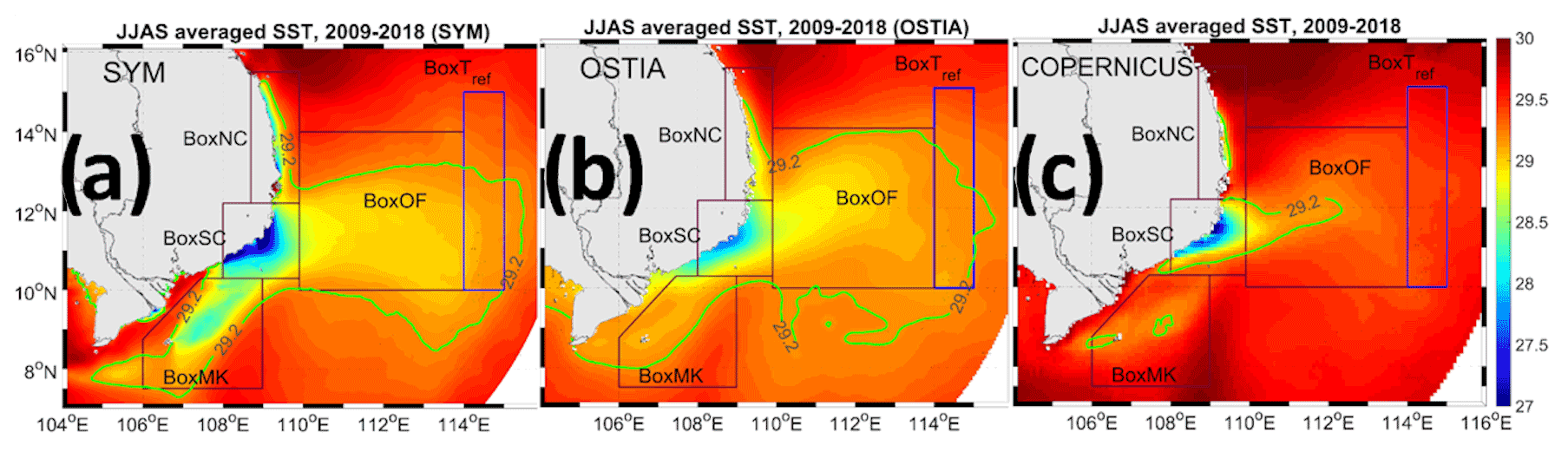
Figure 3JJAS average over 2009–2018 of SST (∘C) from (a) SYMPHONIE, (b) OSTIA, and (c) COPERNICUS over the SVU region. Black boxes show the four upwelling areas, and the blue rectangle shows the reference box. Coordinates of the boxes: BoxNC (12.2–15.5∘ N, 108.7–109.9∘ E), BoxSC (10.3–12.2∘ N, 108–109.9∘ E), BoxOF (10–14∘ N, 109.9–114∘ E), BoxMK (at depth >17 m, 7.5–10.3∘ N, 106–109∘ E), and BoxTRef (10–15∘ N, 114–115∘ E).
To examine the interannual variability of the upwelling over each area, we compute from our simulation an SST-based upwelling index for each box. For that, we followed exactly the same methodology as Da (2018) and Da et al. (2019), who studied in detail the implications of this methodology. To estimate the strength of the upwelling over the area BoxN (which is one of the four boxes defined above), we define the daily upwelling index UId,BoxN:
where ABoxN is the size of BoxN, Tref the reference temperature, and To the threshold temperature. We also define the yearly upwelling index UIy,BoxN:
where NDJJAS=122 d is the duration of the JJAS period. To examine the spatial distribution of the upwelling, we introduce a spatially dependent upwelling index UIy:
To compute Tref, we define a common reference box BoxTref as the area east of the upwelling region that is the less impacted by upwelling (see Fig. 3): Tref is computed as the average JJAS SST over the 2009–2018 period over BoxTref. Using the same Tref for all the four boxes allows us to obtain a continuous spatial field of upwelling index (Eqs. 1, 2, 3) and limits the potential influence of advection of water upwelled in upwelling areas into BoxTref. We obtain Tref=29.20 ∘C. Using again the same method as Da (2018) and Da et al. (2019), the threshold temperature To below which upwelling happens is defined from the analysis of the occurrence of cold surface water: it is defined as the optimal temperature threshold that allows us to cover the largest number of upwelling occurrences but avoids including cold water horizontally advected between upwelling areas. For that, we vary To between 26.0 and 28.0 ∘C every 0.1 ∘C, finally selecting To = 27.6 ∘C.
3.1 Upwelling over BoxMK
To our knowledge, upwelling over BoxMK, referred to as MKU hereafter, has not been detected and studied so far. It was however already visible in AVHRR SST data for 1991–2004 (see Fig. 1 of Da et al., 2019) and in SODA reanalysis SST for 1987–2008 (see Fig. 5 of Fang et al., 2012). The summer surface cooling over BoxMK can actually be observed in OSTIA and COPERNICUS analysis data but with much warmer values than in SYMPHONIE (Fig. 3). This can be explained by the scarce satellite cover over the MKU area and the smoothing associated with the construction of reanalysis data. The percentage of days during which JAXA data are available is shown as an example in Fig. 1d for summer 2018: data availability never exceeds ∼ 85 % over the SCS, is ∼ 75 %–80 % over BoxOF, and is lower than 60 % over BoxMK. To determine if SST cooling really occurs over BoxMK, we thus examine in situ and high-resolution satellite data that cover BoxMK during the period of upwelling.
First, the R/V ALIS crossed BoxMK in June 2014. A surface cooling over BoxMK was indeed observed by ALIS-TSG on 25 June 2014 and simulated by SYMPHONIE, with values of minimum SST ∼ 28.2 ∘C (Fig. 4a, b). On this day, OSTIA and COPERNICUS analysis show a significant cooling in the same area as SYMPHONIE (Fig. 4c–e). However, minimum SST does not go below ∼ 28 ∘C in analysis data, whereas it reaches ∼ 27.5 ∘C in SYMPHONIE. Figure 5a shows the daily time series of minimum SST over BoxMK for SYMPHONIE, OSTIA, and COPERNICUS during summer 2014. All times series show similar temporal variations, with a minimum at the end of June–beginning of July. However, minimum SST values over BoxMK are ∼ 1.5 ∘C lower in SYMPHONIE than in OSTIA and COPERNICUS during this period. Second, Fig. 5b shows the daily time series of minimum SST over BoxMK for SYMPHONIE, OSTIA, COPERNICUS, and JAXA during summer 2018. Again, all time series are following similar variations but with much colder values (by ∼ 1.5 ∘C) in SYMPHONIE than in OSTIA and COPERNICUS. Moreover, values simulated in SYMPHONIE are very close to JAXA observations, with minimum peaks occurring at the same periods: mid-June (∼ 26.6 ∘C), mid-July (∼ 25.6 ∘C), and mid-August (∼ 26.2 ∘C). The spatial coverage of BoxMK by JAXA pixels of quality lever ≥ 4 exceeds 60 % during more than half of the 2018 summer (Fig. 5b), in particular during the periods of low SST (mid-June, middle to end of July, middle to end of August). It is therefore statistically meaningful to use JAXA observations to assess the evolution of minimum SST during the summer period over BoxMK. Figure 6 shows the SST maps during those three upwelling peaks. A surface cooling over BoxMK is produced by JAXA and SYMPHONIE during those peak periods, with SST < 28 ∘C. Again, this surface cooling is also observed by OSTIA and COPERNICUS analysis but with warmer values, although OSTIA also produces a strong cooling during mid-July with minimum SST reaching ∼ 27.5 ∘C. For both summers 2014 and 2018, surface cooling is stronger in SYMPHONIE than in analysis data but occurs over similar areas (Figs. 4, 6).
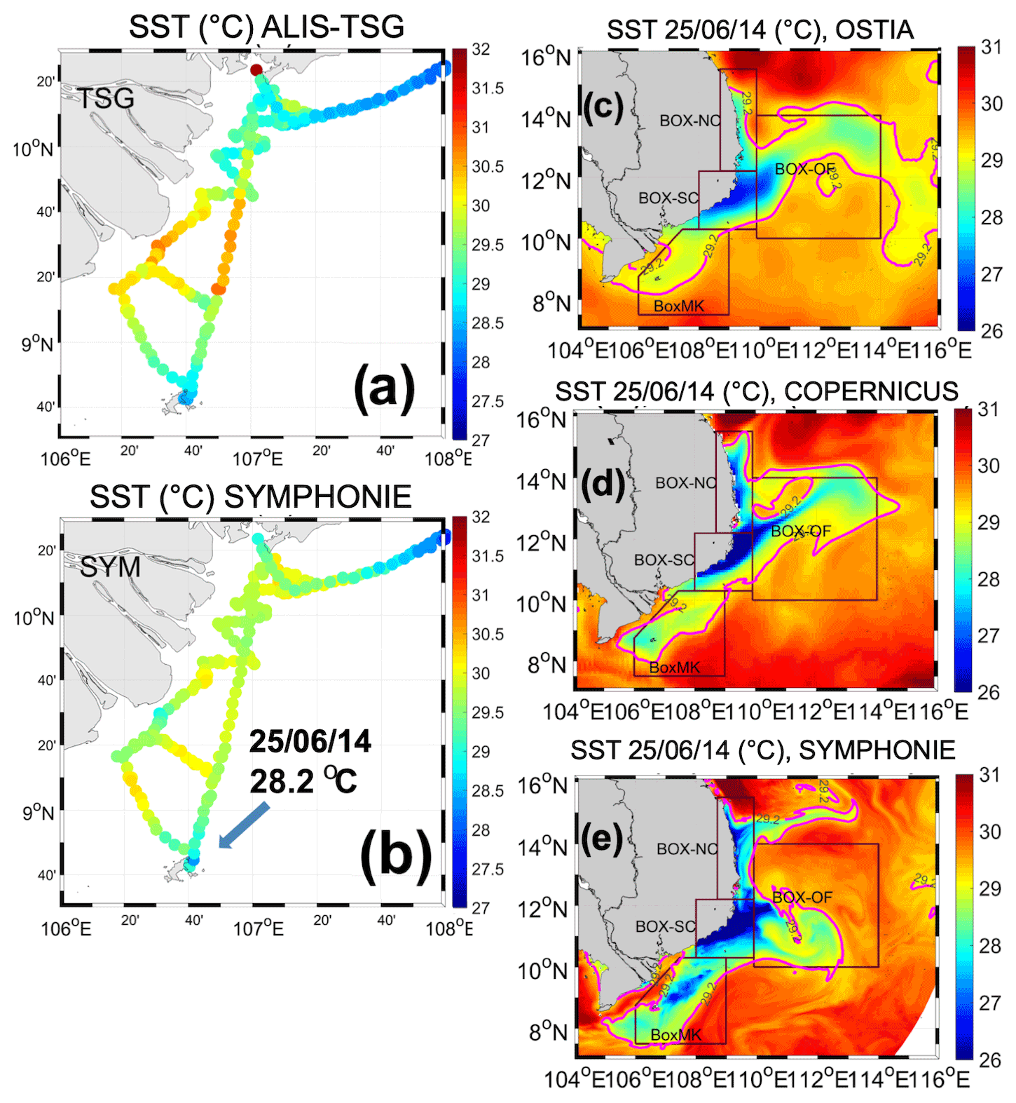
Figure 4Simulated (SYMPHONIE, a) and observed (ALIS-TSG, b) SST (∘C) during the R/V ALIS trajectory offshore of the Mekong mouth in June 2014. The arrow shows the location of minimum SST (∼ 28.2 ∘C both in data and model) recorded near Con Dao islands (∼ 8.6–106.6∘ E) on 25 June 2014. SST on 25 June 2015 (∘C) in OSTIA (c), COPERNICUS (d), and SYMPHONIE (e). The pink contour shows the isotherm Tref = 29.2 ∘C.
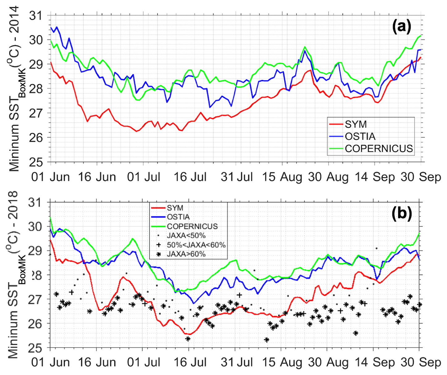
Figure 5Daily time series of minimum SST (∘C) over BoxMK (a) during summer 2014 in SYMPHONIE, OSTIA, COPERNICUS, and (b) during summer 2018 in SYMPHONIE, OSTIA, COPERNICUS, and JAXA. Dots, crosses, and stars correspond, respectively, to a spatial coverage of BoxMK lower than 50 %, higher than 50 %, and higher 60 % for JAXA. We only consider JAXA pixels of quality levels ≥ 4.
This analysis confirms that summer upwelling really occurs over BoxMK. It is captured by ALIS-TSG in situ data and JAXA high-resolution satellite data and simulated accordingly by SYMPHONIE. It is also captured by OSTIA and COPERNICUS but is strongly attenuated. These results therefore highlight the added value of a high-resolution (∼ 1 km at the coast) model to study the upwelling in the SVU area, related to its capability to simulate the fine spatiotemporal-scale structures of SST and surface dynamics better than coarser-resolution gridded satellite data.
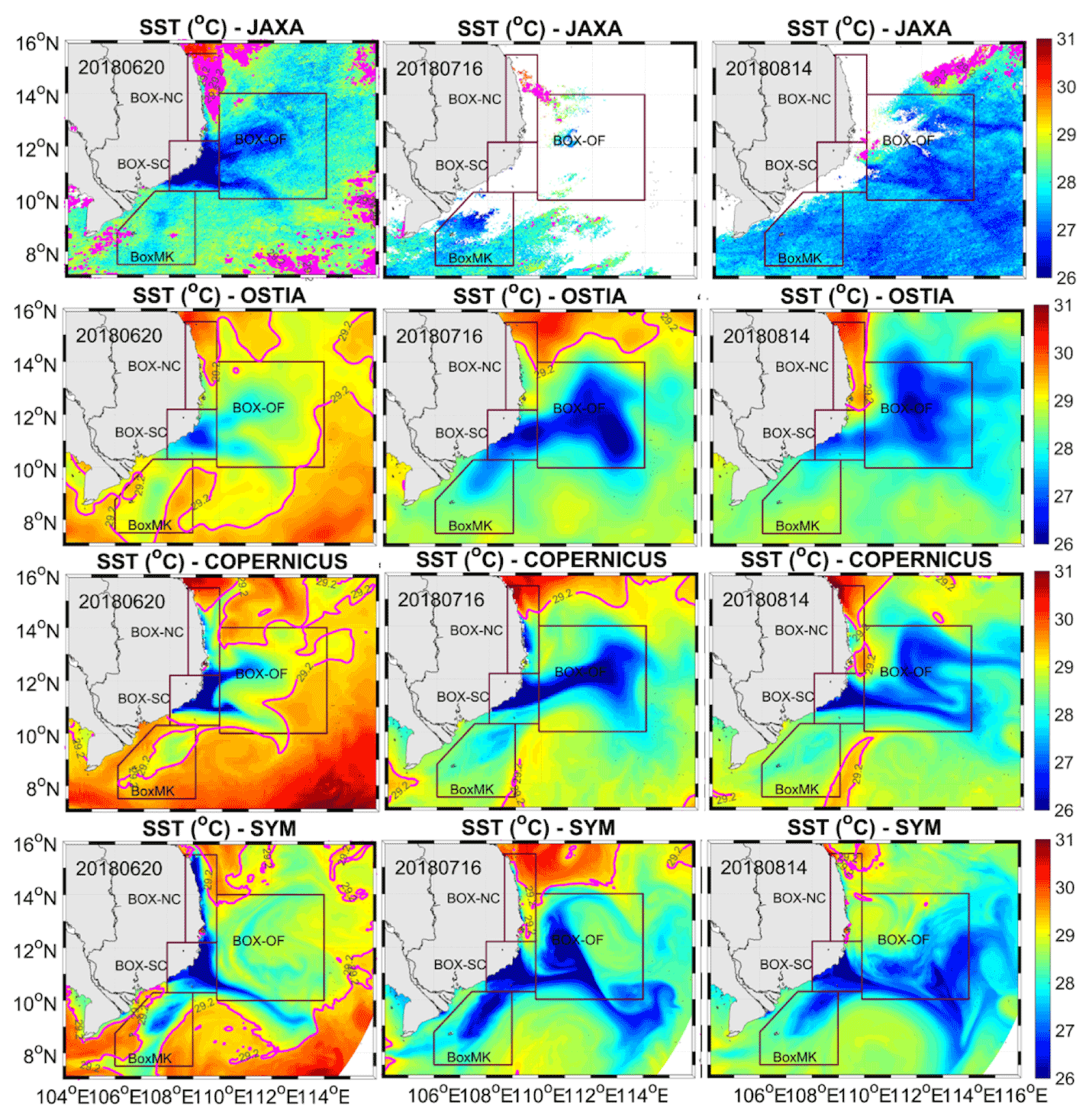
Figure 6Daily SST (∘C) on 20 June 2014 (left), 16 July 2014 (middle), and 14 August 2014 (right) from JAXA (first row), OSTIA (second row), COPERNICUS (third row), and SYMPHONIE (fourth row). The pink contour shows the isotherm Tref.
3.2 Surface circulation, temperature, and salinity in the SCS and SVU regions
Figure 7 shows the time series of climatological monthly averages and of yearly averages of simulated and observed SST, SSS, and sea level anomaly (SLA) averaged over the VNC domain and over the SVU area shown in Fig. 3 (7–16∘ N, 104–116∘ E). In Sect. 3 VNC and SVU regions are called simply VNC and SVU for the sake of conciseness. For both simulated and observed time series, the daily altimetry SLA is obtained by removing at each point the averaged SSH over 2009–2018: . The normalized root-mean square error of a simulated time series compared to an observed time series is computed as , where Si and Oi are, respectively, the simulated and observed values and Omax and Omin the maximum and minimum observed values. Figure 2 shows the maps of winter and summer climatological averages over 2009–2018 of observed and simulated SST, SSS, and SSH.
3.2.1 Annual cycle and seasonal variability of surface circulation, temperature, and salinity
SST seasonal cycles over SVU and VNC are similar (Fig. 7a, g). The seasonal cycle of SST is well reproduced by the simulation. The bias compared to the OSTIA data is equal to 0.08 ∘C with a 0.02 normalized root mean square error (NRMSE) over VNC and to −0.02 ∘C with a 0.01 NRMSE over SVU. The correlation between the simulated and observed SST is highly statistically significant (1.0, p<0.01) for both VNC and SVU. Under the influence of the Southeast Asia Monsoon, SST is at a maximum in May–June and at a minimum in January–February, consistently with Siew et al. (2014). SST spatial patterns are also realistically simulated, with highly significant spatial correlations between simulated and observed fields (Fig. 2a–d, R=0.99 in winter and 0.85 in summer). In winter, the cold atmospheric fluxes and basin-wide cyclonic circulation result in a strong meridional SST gradient. The summer SVU is clearly visible from observed and simulated SST minimum (<28 ∘C). Though SYMPHONIE is in very good overall agreement with OSTIA in terms of spatial variability and temperature range, it however slightly overestimates the observed surface cooling in very coastal areas near Hainan and southern Vietnam coasts. Piton et al. (2021) suggested that this surface cooling could be induced by tides. As explained in Sect. 3.1 when examining the surface cooling over BoxMK and as also shown by Woo et al. (2020), this difference is also due to the SST smoothing in OSTIA and the lower satellite and in situ data availability over the coastal regions (due in particular to the high cloud cover). Other factors could however explain an overestimation of surface cooling in the model: biases in atmospheric fluxes, which are difficult to estimate due to the scarcity of appropriate data; overestimation of vertical mixing due to the numerical model design (schemes of advection and diffusion, vertical coordinates, etc.). The comparison with in situ temperature and salinity profiles however shows the good performance of the model in the representation of water masses characteristics (see Sect. 3.3 below).
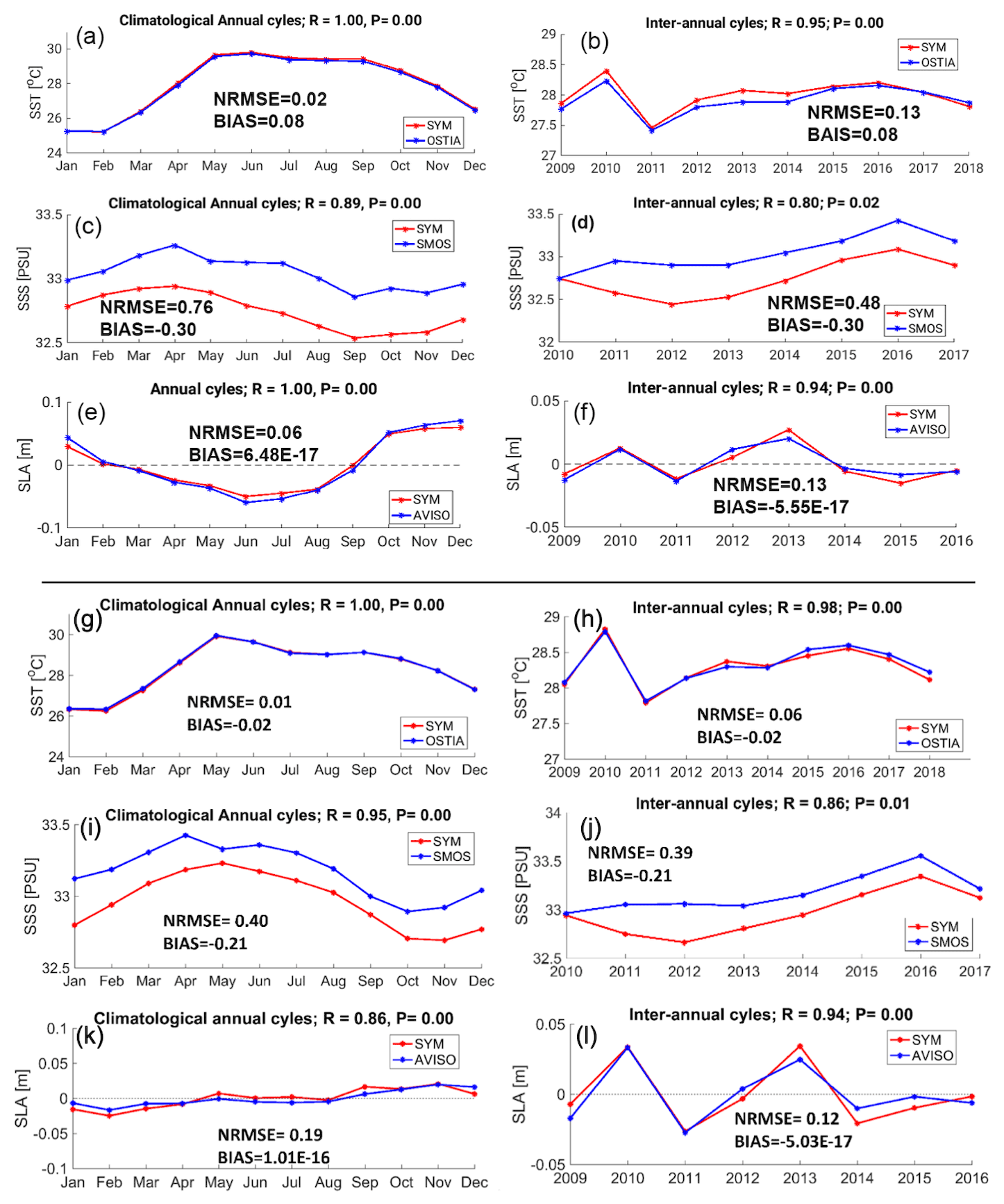
Figure 7Climatological monthly time series (left) and interannual yearly time series (right) of simulated (red) and observed (blue) SST (∘C), SSS, and SLA (meter) averaged over (a–f) the VNC domain and over (g–l) the SVU area (7–16∘ N, 104–116∘ E). Correlation (correlation coefficient R and p value P), NRMSE, and bias of simulated vs. observed values are indicated.
SSS seasonal cycles over SVU and VNC are very similar (Fig. 7c, i). The simulated SSS follows the observed SMOS SSS well, with a highly statistically significant correlation (0.89 over VNC, 0.95 over SVU, p<0.01). Our simulation shows a fresh bias (−0.30 on average over VNC, from −0.22 in winter to −0.36 in summer, −0.21 over SVU) and an associated NRMSE of 0.76 over VNC and 0.40 over SVU. This salinity difference could be due to the coarse resolution of SMOS (28 km) but also to an overestimation of atmospheric freshwater flux in the atmospheric forcing. Spatial patterns are well reproduced, with highly significant spatial correlations between observed and simulated SSS fields (0.84 in winter and 0.88 in summer, p<0.01, Fig. 2e–h). Both simulation and data show low SSS over the Gulf of Thailand and the northwestern Gulf of Tonkin, associated with the strong river and atmospheric freshwater fluxes. In the northeastern SCS, they show high SSS round the year, due to the influence of water entering through the Luzon Strait from the western Pacific Ocean (Qu, 2000; Zeng et al., 2016).
The simulated seasonal cycle of SLA is in very good agreement with AVISO observations (Fig. 7e, k), with a 1.0 correlation coefficient (p<0.01) and a 0.06 NRMSE over VNC and, respectively, 0.86 (p<0.01) and 0.19 over SVU. SLA variations are much weaker over SVU compared to VNC. For VNC, SLA is at a maximum in November–January and at a minimum in June–July, in agreement with studies made from TOPEX/Poseidon altimeter data on the seasonal variability of SLA over the SCS between 1992 and 1997 by Shaw et al. (1999) and Ho et al. (2000). Winter and summer SSH spatial patterns and associated total geostrophic currents are realistically reproduced (Fig. 2i–l), with highly significant spatial correlations between simulated and observed fields (R>0.94). The geostrophic winter circulation is basin-wide cyclonic. The summer circulation is anticyclonic, with a northward alongshore current, composed in particular of an anticyclonic (AC) gyre centered at ∼ 11∘ N and a cyclonic (C) gyre centered at ∼ 13∘ N. These structures form the well-known dipole and associated eastward jet and are highlighted by gray arrows in Fig. 2k–l.
3.2.2 Interannual variability of surface circulation, temperature, and salinity
VNC and SVU regions show very similar interannual chronologies of SST, SSS, and SLA (Fig. 7, right panels).
The interannual variability of SST is very well simulated, with a 0.95 (p<0.01) correlation coefficient and a 0.13 NRMSE compared to the OSTIA dataset for VNC and, respectively, 0.98 (p<0.01) and 0.06 for SVU (Fig. 7b, h). SST shows strong variations over the period, with a 1 ∘C difference between the coldest (2011, 27.5 ∘C over VNC) and warmest (2010, 28.5 ∘C) years. As shown by Yu et al. (2019) over the period 2003–2017, those interannual variations are strongly related to ENSO: the 2010 and 2015–2016 El Niño events induce SST maxima, while the 2011 La Niña event induces an SST minimum.
The simulated interannual SSS time series shows a statistically significant correlation (0.80 over VNC, 0.86 over SVU, p<0.01) and a NRMSE of 0.48 for VNC and 0.39 for SVU compared to SMOS observations (Fig. 7d, j). Both model and data show an increase between 2012 and 2016, also observed by Zeng et al. (2014, 2018). Through a budget analysis based on an SCS 4 km SYMPHONIE configuration over the SCS, Trinh (2020) attributed this salinification to the rainfall deficit during this period.
The interannual variability of SLA is very well simulated, with a 0.94 (p<0.01) correlation coefficient for both VNC and SVU and an NRMSE of, respectively, 0.13 and 0.12 compared to the AVISO dataset (Fig. 7f, l). Both observed and simulated datasets show minimum values in 2009, 2011, and 2015, and maximum values in 2010, 2012, and 2013, with an amplitude of ∼ 3–4 cm.
3.3 Representation of TS characteristics and vertical distribution of water masses at daily to interannual scales
In Sect. 4 below, we use surface variables to quantify the SVU strength and investigate the factors involved in its interannual variability. Surface dynamics are however influenced by the ocean vertical stratification and dynamics. We therefore also assess the capability of the model to realistically reproduce the tridimensional evolution of water masses in the computational area from the open-sea region to the coastal areas. For that, we use the ARGO, GLIDER, IO-18, and ALIS-TSG datasets. We first examine TS diagrams built from ARGO (Fig. 8a), GLIDER (Fig. 8b), and IO-18 (Fig. 8c) observations and co-localized SYMPHONIE outputs.
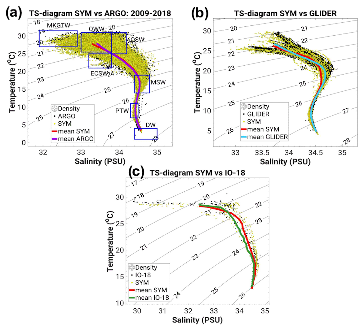
Figure 8TS diagram built from observations from (a) ARGO (black dots and purple line for dot average), (b) GLIDER (black dots, cyan line), (c) IO-18 (black dots, green line), and from SYMPHONIE co-localized outputs (yellow dots, red line). Blue rectangles represent water masses in the SCS (Uu and Brankard 1997, Dippner et al., 2011): MKGTW (Mekong and Gulf of Thailand Water), OWW (Offshore Warm Water), OSW (Offshore Salty Water), ECSW (East China Sea Water), MSW (Maximum Salinity Water), PTW (Permanent Thermocline Water), and DW (deep water).
At the regional scale, ARGO data cover the whole open-sea region over 2009–2018. The TS characteristics of water masses defined by Uu and Brankard (1997) and Dippner et al. (2011) are well reproduced by the model (see Fig. 8 for the acronyms of water masses), with similar contours of simulated and observed scatterplots. In particular the whole range of surface water masses is well simulated, with salinity varying between 32 and 34 and temperature between 20 and 30 ∘C: the fresh MKGTW (Mekong and Gulf of Thailand Water), the more saline OWW (Offshore Warm Water) and OSW (Offshore Salty Water), and the colder ECSW (East China Sea Water). The salinity maximum (reaching ∼ 34.8) of the MSW (Maximum Salinity Water) and the salinity minimum (reaching ∼ 34.4) of the PTW (Permanent Thermocline Water) are also correctly reproduced by the model as well as the DW (deep water) mass.
GLIDER data were collected between January and May 2017, i.e., during the period of northeast monsoon and the transition period to the southwest monsoon. They cover the open-sea region and the coastal area (Fig. 1b). During this ninth year of the simulation, the model is able to reproduce in detail the observed temperature and salinity profiles (Fig. 8b), though with slightly higher biases of salinity (up to 0.15) and temperature (up to 0.4 ∘C) than for the ARGO dataset. In particular it reproduces realistically not only the deep-water masses down to 1000 m depth but also the two branches of surface water masses that were sampled by the glider (Fig. SM1): the fresher branch (SSS < 34.5) observed at the beginning of the glider cruise south of 16∘ N and the warmer branch (reaching 20 ∘C) observed at the end of the cruise north of 17∘ N. SYMPHONIE is therefore able to capture the variability of water masses over the winter to summer transition period, from the coastal areas to the open-sea region, without producing a significant drift after more than 8 years of simulation.
IO-18 and ALIS data were collected during the period and over the region of upwelling, respectively, in 2014 and 2018.
Figure 9 shows the values of observed and co-localized simulated SST and SSS along the ALIS trajectory and their bias. The high-frequency variability of SST and SSS recorded by the TSG along the ALIS trajectory during summer 2014 is very well simulated, with a 0.89 and 0.93 correlation, respectively, between observed and simulated time series. In particular both observed and simulated outputs clearly reveal the surface cooling (by more than 1 ∘C, with water colder than 28 ∘C) and salting (with salinity reaching 34) observed at the end of June–beginning of July 2014 in the SVU area. Comparison with those data therefore shows the ability of the model to reproduce the surface TS characteristics during the period and over the region of upwelling.
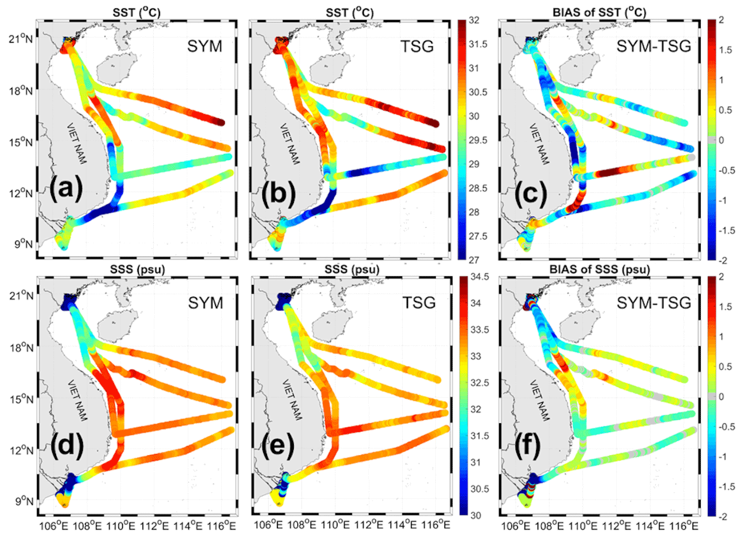
Figure 9Values of SST (top) and SSS (bottom) from (a, d) ALIS-TSG trajectory during summer 2014 and from (b, e) SYMPHONIE co-localized outputs and (c, f) bias between SYMPHONIE and ALIS-TSG.
IO-18 data allow us to explore the vertical dimension of the upwelling region. They covered both the shallow shelf area (8 stations, Fig. 1) and the coastal to offshore upwelling area (10 stations) at the end of summer 2018 (12 to 25 September 2018). Figure 10 shows the simulated and observed vertical TS profiles during IO-18 cruises. The coastal shallow region, subject to the influence of the Mekong freshwater, shows warm (>27 ∘C) and fresh (<34) water, with a halocline between 20 and 10 m, correctly simulated by the model. It corresponds to the nearly horizontal branch of the TS diagram (Fig. 8c). The IO-18 TS diagram and profiles moreover reveal two types of profiles in the deeper regions (i.e., reaching at least 150 m depth), corresponding to the nearly vertical part of the TS diagram. The first type of profiles was sampled along the section at ∼ 12.7∘ N (stations 2.1 to 2.5, located in BoxNC) and in the coastal part of the section along ∼ 10.5∘ N (stations 3.2, 3.4, 3.5, located in BoxSC). It shows high salinities (>34.5) and low temperatures (<25 ∘C) below a pycnocline shallower than ∼ 30 m. It corresponds to locations where upwelling still occurs at this period. The second type of profiles is sampled in the offshore part of the section at 10.5∘ N (stations 3.6 to 3.8, located in BoxOF). It has deeper haloclines and thermoclines, reaching 90 m, with SSS between 32.8 and 33.6 and warmer SST around 28 ∘C: the upwelling had already ceased in this region at this period. Both the TS diagram (Fig. 8c) and the TS profiles (Fig. 10) show that the model is able to reproduce this diversity of TS profiles in the coastal and offshore upwelling regions in very good agreement with IO-18 data, without any significant bias, even after 9 years of simulation.
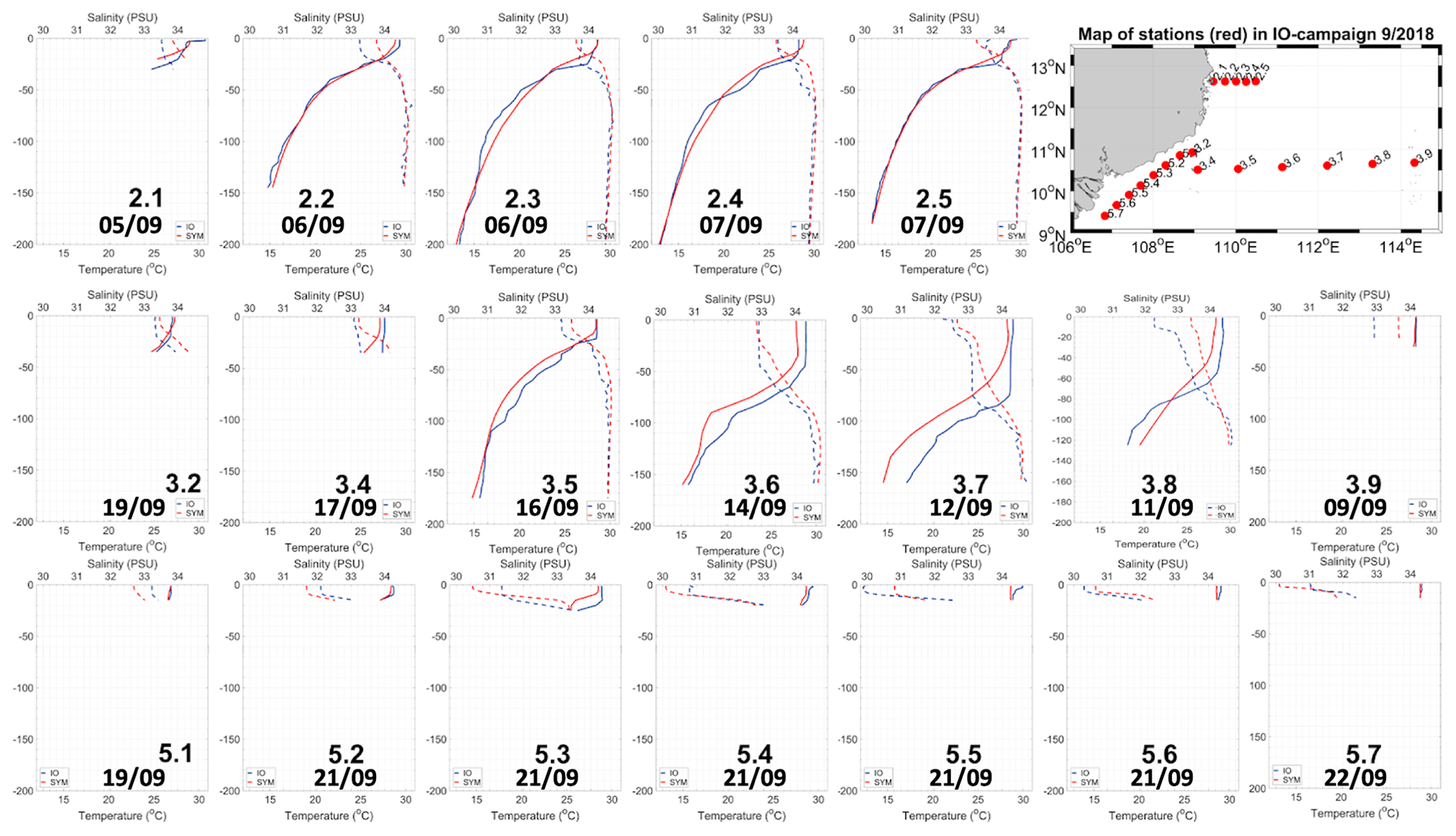
Figure 10Temperature (∘C) and salinity profiles sampled during IO-18 campaign (blue) and simulated by SYMPHONIE (red) between 12 and 25 September 2018. The station and day of sampling are indicated for each profile.
Results of Sect. 3 show that our high-resolution simulation reproduces realistically the surface circulation, temperature, and salinity and the water masses characteristics over the water column and their spatial (from shelf to open sea) and temporal (seasonal to interannual) variability. Based on this 10-year-long simulation, we examine in detail the functioning and interannual variability of SVU over the four regions of interest: the southern (BoxSC) and northern (BoxNC) coasts, the offshore region (BoxOF), and the Sunda shelf (BoxMK).
Figure 11 shows for each summer of the simulation the maps of JJAS-averaged wind stress field and curl over the SVU region computed from ECMWF atmospheric variables. Figure 12 shows the maps of spatial upwelling index UIy and of JJAS-averaged surface current and of its vorticity and the iso-contours of JJAS positive wind stress curl. The surface current vorticity ζ is computed as the vertical component of horizontal surface current rotation: where u and v are, respectively, the zonal and meridional components of the surface current. The surface current is taken as the current of the first layer of the model, whose depth varies from ∼ 1.00 m over most of the domain to ∼ 0.7 m in very shallow and coastal areas. Figure 13 shows the time series of yearly upwelling index over the period 2009–2018 for the four boxes. Table 2 shows the mean and standard deviation of those time series; the coefficient of variation CV is defined as the ratio between the standard deviation and mean. It also shows correlations between time series of significant factors, in particular yearly upwelling indexes, summer wind stress and wind stress curl, and summer surface current vorticity.
Table 2From first to last row: temporal mean and standard deviation of UIy,BoxN over 2009–2018 for each box and coefficient of variation (CV) defined as the ratio between the standard deviation (second row) and mean (first row); mean of JJAS (June–September) average wind stress over each box; mean of integrated positive vorticity over BoxOF; correlations (correlation coefficient and associated p values) between time series of significant factors: yearly upwelling index over each box vs. yearly upwelling index over other boxes vs. JJAS and JA (July–August) average wind stress averaged over each box vs. integrated positive vorticity over BoxOF; average JJAS wind stress over each box vs. average JJAS wind stress over other boxes and vs. integrated positive vorticity over BoxOF; average JJAS wind stress curl (WSC) over each box vs. average JJAS wind stress over other boxes and vs. integrated positive vorticity over BoxOF. Correlations significant at more than 95 % (p<0.01) are highlighted in bold.

4.1 Interannual variability of wind and offshore summer circulation
4.1.1 Relationship between wind stress and wind stress curl
The intensity of wind and wind stress curl shows a strong interannual variability (Figs. 11, 13), but their spatial patterns are quite similar from one year to another and related to the summer monsoon wind. A wind stress curl dipole develops offshore of Vietnam, with an area of strong positive curl along and off the Vietnam coast in the north (covering BoxSC and a part of BoxOF and BoxNC) and an area of strong negative curl in the south (covering BoxMK).
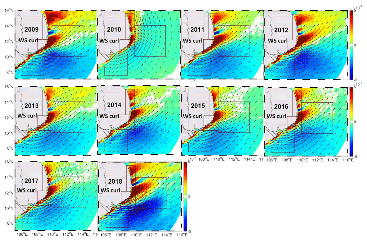
Figure 11Maps of JJAS-averaged wind stress (arrows, N m−2) and wind stress curl (colors, N m−3) for each year of the simulation.
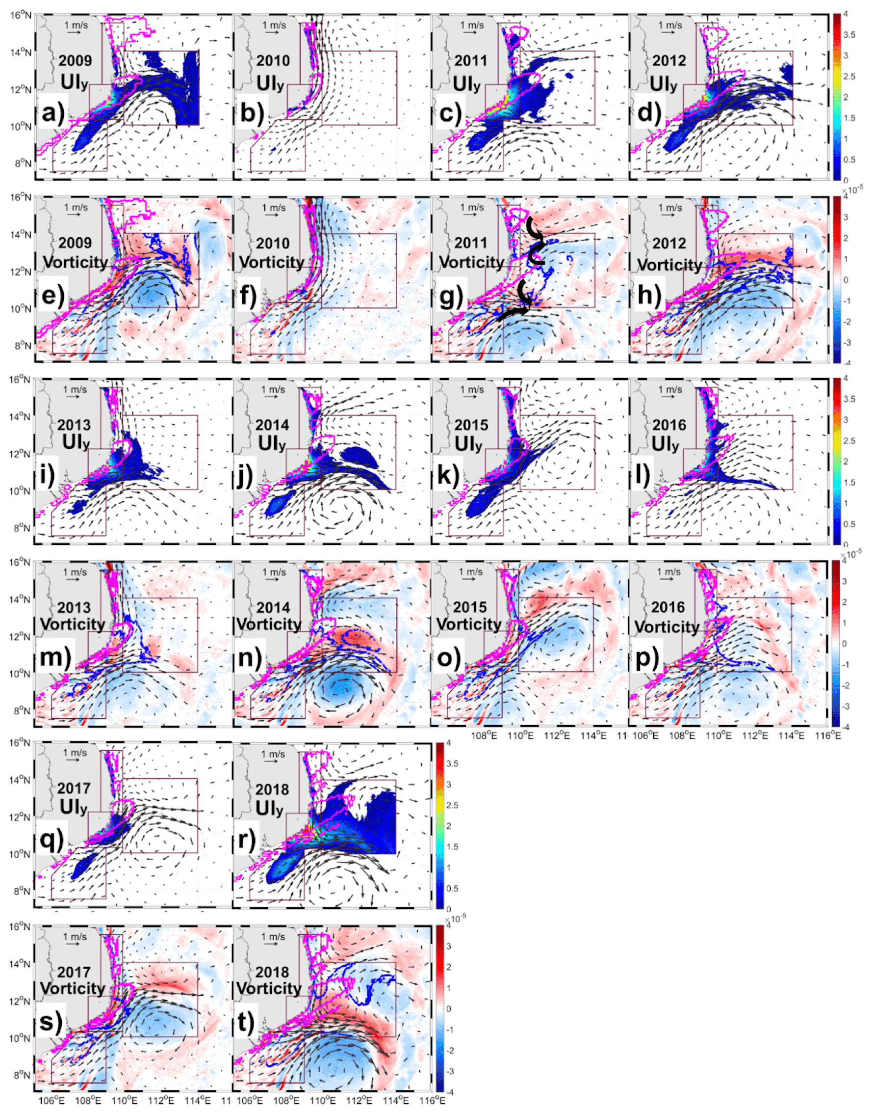
Figure 12Maps of spatial yearly upwelling index UIy (∘C, a, b, c, d, i, j, k, l, q, r) and of speed and direction (arrows, m s−1) and vorticity (colors, s−1) of JJAS-averaged surface current (e, f, g, h, m, n, o, p, s, t) for each year of the simulation. Pink contours show the +3.10−7N m−3 isoline of JJAS average positive wind stress curl. Blue contours show the 0.1 ∘C isoline of UIy.
Figure 13 shows the yearly time series of the average over each box of JJAS wind stress, WSJJAS,BoxN. Interannual time series of the summer wind stress over BoxSC and BoxMK are almost equal to the summer wind stress over BoxOF and completely correlated with it (correlation higher than 0.96, p<0.01, Table 2). The intensity and interannual variability of summer wind intensity over BoxSC and BoxMK coastal areas is thus completely driven by the large-scale summer monsoon wind intensity over the region. The averages of JJAS wind stress curl over BoxSC (area of maximum positive wind stress curl) and BoxMK (area of maximum negative wind stress curl) are indicators of the intensity of the wind curl dipole that develops offshore of Vietnam. There is a highly significant correlation (absolute value greater than 0.91, p<0.01, Table 2) between these indicators on one side and the wind stress on BoxMK, BoxSC, and BoxOF on the other side. The intensity of wind stress over those three regions of upwelling and the intensity of the wind stress curl dipole are therefore strongly related. By contrast, wind stress and wind stress curl over BoxNC are not significantly correlated with wind over any of the other boxes (Table 2).
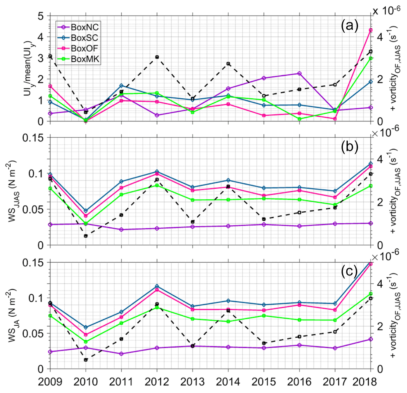
Figure 13Interannual time series of normalized yearly upwelling index (first row), average JJAS (second row), and JA (third row) wind stress (N m−2) over each upwelling box (BoxNC: purple; BoxSC: blue; BoxOF: pink; BoxMK: green). The black dashed curve shows the integrated positive summer surface current vorticity over BoxOF (s−1).
4.1.2 Relationship between wind and offshore summer circulation
Positive surface summer current vorticity develops over the SVU region along the northern flank of the eastward jet (a more intense and narrow jet being characterized by a higher vorticity) and in the area of cyclonic activity north of the jet (Fig. 12). We compute the time series of , the spatial integral over BoxOF of the positive part of JJAS-averaged relative vorticity (Fig. 13). integrates both the cyclonic activity north of the jet and the positive vorticity on the northern flank of the eastward jet. It is thus an indicator of the intensity of the cyclonic part of the summer circulation (ACC dipole + eastward jet) in the offshore region. The interannual variability of is strongly induced by the variability of intensity of wind stress and of the wind stress curl dipole. There is a highly significant correlation between the time series of and the time series of wind stress over BoxSC and BoxOF (0.89, p<0.01, Table 2) and of wind stress curl over BoxMK and BoxSC (−0.81 and −0.82, p<0.01, respectively).
4.2 BoxSC
The interannual variability of SCU is significant, although it is the lowest of the four boxes (CV = 53 %, Table 2). In 2010, WSJJAS,SC is at a minimum and significantly weaker than for the other years and almost no upwelling develops over BoxSC (UI ∘C, 1 order of magnitude smaller than the average). Conversely, when wind stress peaks in 2018 (WSJJAS≃0.11 N m−2, Fig. 13) SCU reaches its maximum intensity (UI ∘C, almost twice stronger than the average). We obtain a highly significant correlation between UIy,SC and WSJJAS,SC (R=0.85, p<0.01, Table 2). UIy,SC is also significantly correlated with (0.60, p=0.07, Table 2), which confirms that SCU is stronger (weaker) for years of intense (weak) summer circulation off the Vietnam coast. Our results therefore confirm conclusions from previous lower-resolution studies (see the Introduction): the interannual variability of SCU is driven at the first order by the intensity of the summer-averaged monsoon wind over the region and by the intensity of the regional summer circulation.
Our study moreover reveals that other factors than the summer average of wind intensity contribute to the interannual variability of SCU, namely intraseasonal wind chronology and mesoscale circulation over BoxSC.
First, the daily to intraseasonal variability of wind forcing contributes to the summer average of SCU intensity. For example, even though 2009 and 2012 show the same average summer wind over BoxSC (WS N m−2), SCU is 25 % weaker in 2009 (UI ∘C) than in 2012 (UI ∘C). Figure 14 shows the time series of daily upwelling index UId,SC and of daily average wind stress over BoxSC for 2009 and 2012 (and 2011). For both years, the development of SCU is related to the daily chronology of wind, with upwelling peaks occurring during wind peaks. The wind over BoxSC is stronger in July and September for 2009. It is stronger in June and August for 2012. In 2012, the SCU consequently develops strongly in June and persists throughout the summer, especially in August. Conversely in 2009 the SCU mainly develops in July and does not persist in August due to the weaker wind during this month. The daily to intraseasonal variability of wind forcing during the summer therefore contributes to the summer average of SCU intensity and hence to the SCU interannual variability.
The second factor that influences the summer average SCU intensity is the mesoscale circulation over the coastal area. For example, 2011 shows the second strongest SCU (UI ∘C), ∼ 90 % stronger than for 2009 and ∼ 40 % than for 2012 (Fig. 13). The SCU develops strongly in June 2011 and persists throughout the summer, reaching much higher values than in 2009 and 2012 (Fig. 14). However, WSJJAS,SC in 2011 (≃ 0.09 N m−2) is ∼ 10 % lower than in 2009 and 2012. Moreover, wind stress in June 2011 is slightly weaker than in June 2009 and 2012 on average over the month (Fig. 14). Figure 14 show that it also does not differ in terms of the maximum intensity of high-frequency peaks, though the chronology of those peaks differs. This shows that the higher upwelling intensity in 2011 does not result from a difference in summer wind, neither on average nor at the daily to intraseasonal scales. Instead, it results from the ocean circulation. The years of 2009 and 2012 show the ACC dipole and associated eastward jet at ∼ 12∘ N described in the literature (Fig. 12e, h). Instead, during summer 2011, two ACC structures develop along the Vietnamese coast, as can be seen in Fig. 12g where they are highlighted by black arrows. These structures are associated with two eastward jets departing from 10 and 13.5∘ N. This results in an overall outward current along the coast and hence in a wider coastal upwelling. The coastal circulation and mesoscale circulation are therefore a second factor that contributes to the summer average of SCU intensity and to its interannual variability.
4.3 BoxOF
OFU shows the strongest interannual variability (CV ≃ 126 %, Table 2), explained partly by the very strong OFU in 2018 compared to other years induced by the strong wind in summer 2018 (Fig. 13). The interannual chronology of OFU is very similar to that of SCU, with a minimum in 2010 and a maximum in 2018, and UIy,SC and UIy,OF are highly significantly correlated (0.73, p=0.02, Table 2).
Our results first confirm that summer wind strength is a key factor involved in OFU interannual variability: UIy,OF and WSJJAS,OF are highly statistically significantly correlated (R=0.77, p=0.01, Table 2). They also confirm the link between the intensity of OFU and of summer offshore circulation and related vorticity, with a significant correlation between the time series of UIy,OF and (0.69, p=0.03, Table 2). Figure 12 indeed reveals that OFU indeed occurs mainly in areas of positive surface current vorticity: along the northern flank of the eastward jet and north of the jet as the result of mesoscale cyclonic structures. For some cases, as suggested by Da et al. (2019) and Ngo and Hsin (2021), OFU can even be inhibited. In 2010 upwelling practically does not develop over BoxOF and BoxSC (Figs. 12, 13). The usual eastward offshore jet and dipole structure do not exist during summer 2010 (Fig. 12). is indeed much smaller than for the 9 other years (Fig. 13, equal to s−1 vs. s−1 on average, Table 2). Moreover, an alongshore northward current flows between 9 and 16∘ N (Fig. 12). Those circulation conditions prevent the formation of an offshore current and of the associated upwelling. For this year, extreme weak wind conditions as well as circulation patterns thus both prevent the development of upwelling.
Our study moreover reveals again that factors other than summer wind intensity and summer circulation over the offshore area contribute to the interannual variability of OFU. For example, in 2018, the intensity of both wind and circulation is only ∼ 10 % higher than in 2009 and 2012 (Fig. 13): in 2018, WSJJAS,OF and are equal to 0.11 N m−2 and s−1 vs. 0.10 N m−2 and s−1 in 2009 and 2012. However, UIy,OF in 2018 is, respectively, 2.6 and 4.6 times larger than in 2009 and 2012 (0.32 ∘C vs. 0.12 and 0.07 ∘C) and 4 times higher than the average (0.07 ∘C, Table 2). Comparatively, for BoxSC, UIy,SC in 2018 is only twice larger than the average value. Last, the correlation between UIy,BoxN and WSJJAS,BoxN is lower for BoxOF (0.77, Table 2) than for BoxSC (0.85). This suggests that the influence of factors others than summer-averaged wind and circulation on the interannual variability of OFU could be more important than for SCU.
The intraseasonal variability of wind is an important factor that contributes to the summer average of OFU intensity and hence to its interannual variability. Figure 15 shows the time series of daily upwelling index UId,OF and daily average wind stress over BoxOF for 2009, 2012, and 2018. Wind stress peaks mostly occur in July and September in 2009 and in June and September in 2012. In contrast, in 2018, wind stress peaks occur in July and August, inducing a very strong upwelling during those months. The monthly averaged wind is consequently significantly stronger in July and August 2018 than in July and August of the other years and than in June and September 2018 (Fig. 15). This suggests that the summer intensity of OFU is higher when wind peaks occur during the core of the summer season (July–August) than at the beginning (June) or end (September). The correlation of time series of UIy,OF with time series of July–August averaged wind stress over BoxOF is indeed higher (0.84, p<0.01, Table 2) than the correlation with JJAS wind stress (0.77, p<0.01), confirming this hypothesis. Strong wind stress during July–August thus favors the development of OFU, more than during June and September. This is presumably related to a favorable combination of wind forcing and offshore circulation during this period. Conversely, for BoxSC, the correlation between UIy,SC and WSJA,SC is weaker than for WSJJAS,SC (0.70, p=0.03 for WSJA,SC vs. 0.85, p<0.01, for WSJJAS,SC, Table 2). The development of SCU does indeed occur during the whole JJAS period as soon as the wind conditions are favorable and is thus mainly induced by wind forcing which prevails over and drives circulation patterns (see Sect. 4.2).
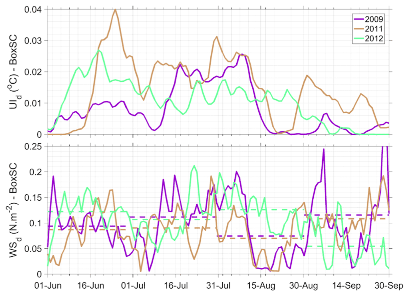
Figure 14Time series of daily upwelling index (top) and average daily (plain line) and monthly (dashed line) wind stress (bottom) over BoxSC between June and September for years 2009 (purple), 2011 (orange), and 2012 (green). For the sake of readability, the y axis is cut off for the last extreme value of September 2009, which corresponds to the passage of storm Ketsana over the SVU region (see the NOAA storm track website at https://coast.noaa.gov/hurricanes, last access: 25 July 2022).

Figure 15Same as Fig. 9 for BoxOF and years 2009 (purple), 2012 (green), and 2018 (magenta). For the sake of readability, the y axis is cut off for the last extreme value of September 2009, which corresponds to the passage of storm Ketsana over the SVU region (see the NOAA storm track website at https://coast.noaa.gov/hurricanes, last access: 25 July 2022).
4.4 BoxNC
Upwelling also develops, though to a weaker extent, along the northern part of the central Vietnam coast (BoxNC). UIy,NC shows a relatively strong interannual variability (71 %, Table 2). We obtain no statistically significant correlation between the UIy,NC time series and the time series of the average wind stress, whatever the period and area of averaging (Table 2). Moreover we obtain no statistically significant correlation between the UIy,NC time series and the upwelling index over the three other boxes (Table 2). This suggests that contrary to SCU and OFU, the interannual variability of NCU is not driven by the summer wind or the summer offshore circulation. Examining in detail the 10 summers of the simulation in Fig. 12, we show instead that the development of NCU is inhibited or favored depending on the circulation that prevails over BoxNC.
Ngo and Hsin (2021) examined the role of each component of the summer wind in the development of NCU. Following their analysis, Fig. 16 shows the maps of correlations between yearly time series of UIy (for SCU, NCU, and OFU) and JJAS wind stress intensity over BoxOF on one side and the (spatially dependent) times series of JJAS wind stress components and intensity on the other side. First, the intensity of JJAS wind stress over BoxOF is highly significantly positively correlated (p<0.01) with the components and the intensity of wind stress over most of the domain (Fig. 16e). But it is negatively correlated with the zonal component and the intensity of wind stress in the northeastern part of the domain (including BoxNC). The intensification of the summer monsoon wind over the region is thus associated with an intensification of the wind over most of the area but with a weakening of its intensity and meridional component, i.e., a less northward and more eastward direction, in the northwestern part and vice versa. Second, correlation maps for OFU and SCU are very similar to the correlation maps for JJAS wind stress intensity over BoxOF, with larger areas of highly significant correlations for SCU than for OFU (Fig. 16c, d, e). This confirms the link shown in Sect. 4.2 and 4.3, stronger for SCU than for OFU, between the intensity of upwelling over those regions and the intensity of monsoon wind. Third, the correlation maps for NCU are of opposite signs to the other maps (Fig. 16a). When the summer monsoon wind intensifies (favorable to SCU and OFU), the wind stress and its meridional component weaken in the northeastern region covering BoxNC. The wind is therefore more eastward, i.e., less parallel to the coast, and more offshore, i.e., not favorable to NCU. It is the opposite when the summer monsoon wind weakens. Last, correlations are much more statistically significant (p<0.01) for SCU and, to a lesser extent, OFU, than for NCU (p<0.05 or 0.01 only in very small coastal areas over BoxNC). These results therefore suggest that wind also participates to the interannual variability of NCU, with favorable conditions opposite to those favorable to SCU, OFU, and MKU, as already shown by Ngo and Hsin (2021). However, they further reveal that this influence of wind is not as important as for the other areas and suggest that other factors may be playing roles of equal or stronger importance, in particular OIV and mesoscale structures.
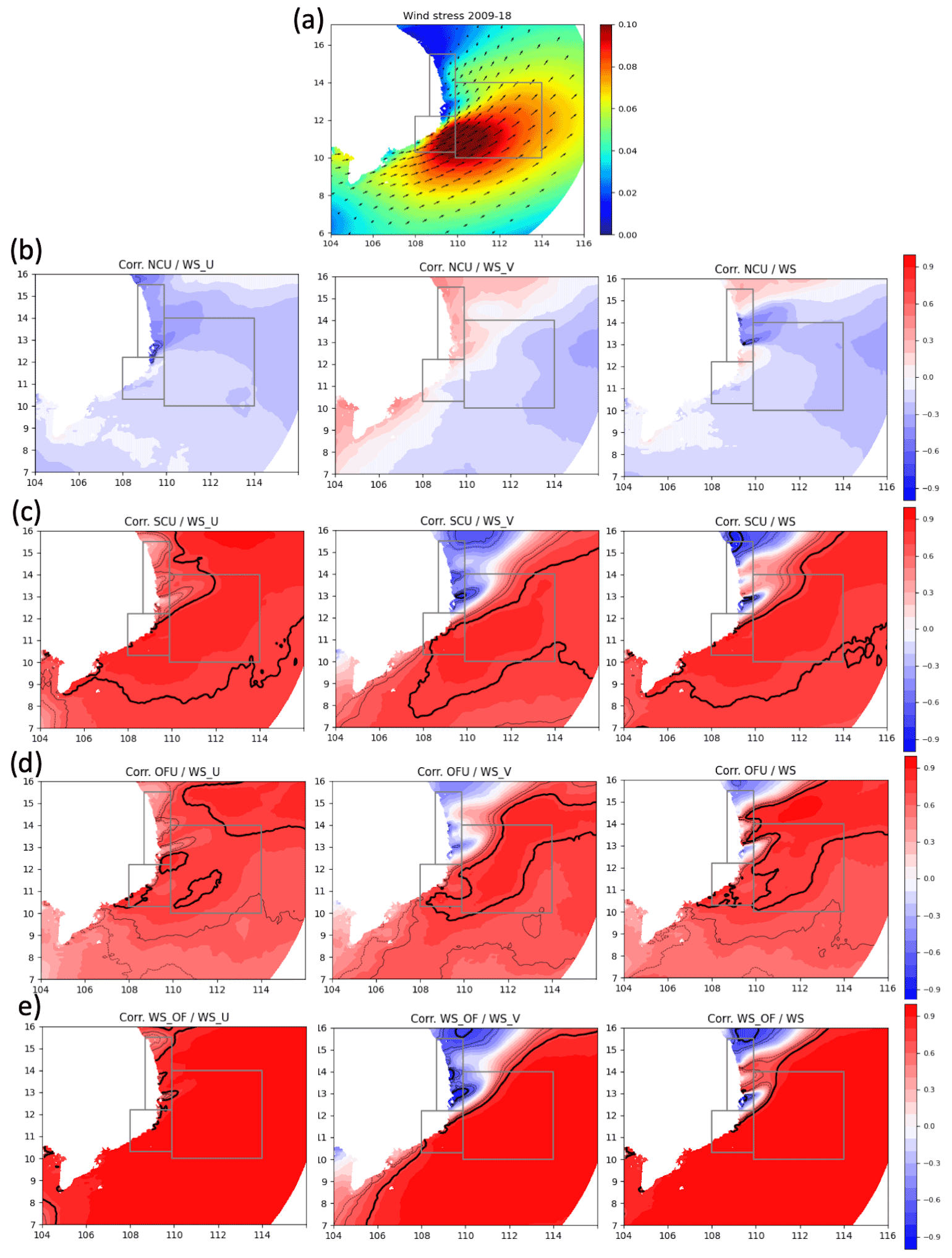
Figure 16(a) Direction (arrows) and intensity (N m−2) of average JJAS wind stress over the SVU area during 2009–2018 from ECMWF analysis. Panels (b) to (e): correlation between yearly time series of the zonal (left) and meridional (middle) components of wind stress and of its intensity (right) and (b) UIy,NC, (c) UIy,SC, (d) UIy,OF, and (e) JJAS wind stress intensity over BoxOF. Thick, plain, and dotted lines correspond, respectively, to the isolines p = 0.01, p = 0.05, and p = 0.10.
Examining the spatial patterns of circulation indeed shows that they strongly impact the NCU development. The NCU is inhibited when alongshore currents, either southward or northward, prevail over BoxMK. Southward alongshore currents prevail during summers of strong wind over the SVU region, when the ACC dipole and eastward jet, and hence positive vorticity , are highly marked, inducing strong OFU and SCU (see summers 2009, 2012, 2018, Figs. 12, 13). These southward currents are associated with the western part of the northern cyclonic gyre and a divergent circulation and hence with a coastward component and a coastal downwelling which inhibits the NCU. Northward alongshore currents prevail during years of weak or average wind over the region (see summers 2010, 2013, 2017). During those years, offshore circulation (ACC dipole and eastward jet) is average (2017), weak (2013), or even absent (2010), resulting in weak average Ekman transport and pumping and hence in weak SCU and OFU. The weakness of the offshore circulation allows the development of an alongshore northward current all along the Vietnamese coast, which also inhibits the NCU. Southward or northward alongshore currents over BoxNC therefore result from two opposite situations in terms of wind and offshore circulation but induce both NCU inhibition.
The NCU is enhanced when offshore-oriented circulation prevails over BoxMK. Offshore-oriented circulation can result first from the development of a secondary dipole north of the usual dipole structure: see the alternation of negative and positive vorticity between 12 and 16∘ N along the coast (Fig. 12) for summers 2011, 2014, and 2015. This secondary dipole is associated with a second coastal area of convergence over BoxNC and hence a secondary eastward jet that induces the strong NCU. This situation is not related to the intensity of summer wind or offshore circulation (Figs. 12, 13). Indeed it occurs both for summers with wind slightly stronger (2011 and 2014) or weaker than average (2015) and with strong (2014) or weak (2011, 2015) offshore circulation. Offshore-oriented circulation also develops when a weaker but wider than average eastward jet prevails over a large part of the coastal region, including BoxNC (see summer 2016). This results in the offshore advection of cold water all along the coast and hence in the development of a stronger than average NCU. NCU is therefore favored by the development of offshore-oriented currents along the coast that result from a favorable spatial organization of submesoscale to mesoscale dynamics.
4.5 BoxMK
MKU shows the weakest mean value of the four boxes (<0.07 ∘C, Table 2) and a relatively strong interannual variability (CV = 85 %). The interannual chronology of MKU is very similar to that of OFU and SCU, with a minimum in 2010 and a maximum in 2018 (Fig. 13). UIy,MK is highly significantly correlated with UIy,SC (0.83, p<0.01, Table 2) and UIy,OF (0.92, p<0.01). MKU interannual variability is therefore likely driven by the same factors as OFU and, to a slightly lesser extent, SCU. As for SCU and OFU, the summer wind strength and summer offshore circulation are indeed key factors involved in MKU interannual variability. UIy,MK shows a highly statistically significant correlation with summer wind over the region (WSJJAS,SC: 0.83, p<0.01, Table 2) and with the offshore circulation (: 0.74, p=0.01). This correlation with is even higher than for SCU (0.60) and OFU (0.69), suggesting an even stronger influence of summer offshore circulation (eastward jet and ACC dipole) in MKU interannual variability.
MKU develops in the area of positive vorticity along the western flank of the northeastward current that flows off the Mekong Delta (Fig. 12). Its intensity is stronger when this current and the associated positive vorticity are stronger. This current constitutes the western part of the southern anticyclonic gyre of the ACC dipole (Fig. 12). It forms the eastward jet when it encounters the northern cyclonic gyre. The intensity of this current therefore varies interannually following the intensity of the summer offshore circulation induced by summer monsoon wind. This explains the significant correlation between MKU and the regional offshore circulation and wind.
In contrast with upwelling that develops over the three other areas, the position of MKU is very stable from one year to another (Fig. 12). MKU develops every year in the same area of positive current vorticity, though with very different intensities (absent in 2010 and 2016 to very strong in 2018). This clearly distinguishes it from the upwelling that develops in the other zones, in particular NCU and OFU, whose position is highly variable. The spatial structure of surface currents and associated vorticity in the MKU region is also very stable from one year to another (Fig. 12), which explains this stable position of MKU. This agrees with conclusions from Fang et al. (2012), who showed that this segment of the summer circulation is stable at the interannual scale, whereas the northern and eastern parts are much more unstable. This stable circulation spatial pattern over BoxMK could be explained by the fact that it may be constrained by factors that do not vary interannually, such as topography and tide. BoxMK is indeed located on the shallow continental shelf, with depths varying from ∼ 15 m at the coast to more than 200 m over the continental slope (Fig. 1c).
These results show that MKU interannual variability is driven first by the summer monsoon wind and by the northeastward current, which is completely related to the intensity of the wind-induced summer offshore circulation. MKU develops in an area of positive vorticity associated with the northeastward coastal current in BoxMK. The spatial structure of this current and hence of MKU is interannually stable, presumably because it may be strongly constrained by bathymetry-related mechanisms.
5.1 Sensitivity to the choice of varying vs. constant reference temperature Tref
To compute the daily to yearly upwelling intensity, a constant reference temperature Tref was used (see Sect. 2.3), as done previously by Da et al. (2019). Our choice of a constant Tref was based on the fact that even if the reference box was chosen as far as possible from the upwelling area and over the same latitudinal region, this choice was constrained by the computational domain (location of eastern boundary, Fig. 3). On average, BoxTref is outside of the upwelling area; however it can be influenced by the eastward advection of cold surface water upwelled in the other boxes, especially for years of strong upwelling. This advection is for example visible during summer 2018 of very strong OFU and not during summer 2010 of weak OFU (Fig. 17a). It results in a colder JJAS average SST over BoxTref in 2018 and more generally in years of strong OFU (2009, 2011, 2012, and 2018, Fig. 1b) than in 2010. Using an interannually varying SST could thus result in weaker yearly upwelling indexes for years of strong OFU. Using a climatological constant Tref contributes to limit this effect. Conversely, other studies used an interannually varying Tref to take into account the fact that SST over the SCS varies on an interannual basis (e.g., Ngo and Hsin, 2021): the summer SST over the SCS is indeed also affected by other factors than the SVU, in particular by large-scale factors like ENSO, with a warmer sea surface following El Niño events (Qu et al., 2004; Wang et al., 2006). Taking into account the effect of those large-scale factors justifies the use of a yearly varying Tref as done by Ngo and Hsin (2021). Previous studies however also showed that ENSO influences the SVU, with weaker SVU following El Niño events (Da et al., 2019) and hence weaker advection of cold water. Choosing a constant or a yearly varying Tref therefore involves tradeoffs between those influence factors. Note that the choice of a seasonally average vs. a daily varying Tref involves similar tradeoffs (taking into account or not the effect of lateral advection vs. seasonal variability). We evaluated the influence of a varying Tref on our results, computing upwelling indexes with an interannually varying Tref instead of a constant Tref (Fig. 17b). The yearly time series of upwelling indexes UIy,BoxN differs very slightly, in particular for stronger values as expected (see year 2018), but changes are not significant. Recomputing all the variables from Table 2 (table not shown for the sake of conciseness) shows that the interannual variability is only slightly reduced and that correlation coefficients consequently also slightly decrease but by less than ∼ 0.10. In particular, correlations that were statistically significant (or not) remain statistically significant (or not). Our results and conclusions are therefore robust to the choice of an interannually varying vs. constant Tref.

Figure 17(a) Maps of JJAS-averaged SST in 2010 and 2018 in the 2009–2018 simulation (∘C). Panel (b) (first row): yearly time series of the JJAS-averaged SST over the reference box for each year (i.e., varying Tref, full black line). The dashed line shows the value of the climatological summer-averaged SST over the reference box (i.e., constant Tref). Panel (b) (second to fifth row): yearly time series of upwelling indexes UIy computed using a varying (red) vs. constant (blue) Tref for BoxNC, BoxSC, BoxOF, and BoxMK.
Last, we investigated the effect of using a common Tref for the four boxes instead of using a specific Tref for each box. For that, we used for each area a reference temperature equal to the average SST over an area contiguous to each box (figures not shown). Results show that using a common vs. specific Tref can influence the values of the upwelling index but only by up to 20 % for BoxNC. Moreover, this does not have any significant influence on the indicators and correlations shown in Table 2: results changed by less than 1 % when testing this choice. Our results are therefore also robust to this choice.
5.2 Role of intraseasonal variability of atmospheric forcing
We confirmed in Sect. 4 the leading role of the seasonal average of summer monsoon wind in the interannual variability of the yearly intensity of SCU, OFU, and MKU. We moreover showed in Sect. 4.2 and 4.3 that the intraseasonal chronology of wind stress influences the summer average of SCU and OFU intensity and their interannual variability: for a similar average summer wind, OFU is stronger if wind peaks occur during the July–August period. However other factors may be involved. Indeed, the monthly wind stress over BoxOF is stronger in June and August in 2012 than in 2009 and similar in July, and is similar. However, OFU is 50 % weaker in 2012 than in 2009 (Figs. 13, 15). A first factor explaining this difference is the daily wind chronology inside the July–August period: 2009 shows two distinct periods of wind maximum in mid-July and mid-August, whereas 2012 shows two close peaks during the second half of July (Fig. 15). These results suggest that the wind chronology not only at the intraseasonal monthly scale but even at the daily scale inside the July–August period affects the upwelling development. In particular wind peaks need to be sufficiently spaced in time. This result is supported by previous studies (Xie et al., 2007; Liu et al., 2012) which highlighted the importance of intraseasonal wind peaks on SVU development.
This conclusion was obtained from the study of four summers (2009, 2011, 2012, and 2018). To quantitatively highlight this role of wind peaks, we performed an additional simulation from June to September 2018 (the summer that shows the strongest wind stress and upwelling over BoxSC, BoxOF, and BoxMK, Fig. 13): during the whole summer, we used a temporally constant wind stress, computed for each point of the model as the JJAS 2018 average of the daily wind stress. Initial conditions for this simulation were taken as the conditions of 1 June 2018 of the 2009–2018 simulation. In the sensitivity simulation, the surface cooling is much weaker than during summer 2018 of the 2009–2018 simulation, and no upwelling develops on any of the boxes during the whole summer. This result quantitatively highlights the fundamental role of wind intraseasonal variability in the development of upwelling and in its summer average intensity: a constant wind, even of strong average value, is not sufficient for the development of SCU, OFU, and MKU, and peaks of strong winds are essential. This simulation and additional sensitivity tests will be examined in more detail in further studies.
Additional simulations would now be required to more quantitatively assess the role of intraseasonal variability vs. the seasonal and monthly average of wind stress in the yearly upwelling intensity. In particular, ensembles of simulations with wind of same seasonal average but different daily chronology, and the reverse, would help to estimate the variability of summer average upwelling induced by the variability of the intraseasonal chronology vs. by the interannual variability of summer average wind.
5.3 Role of forced vs. chaotic variability
The interannual variability of the offshore circulation is partly driven by the intensity of regional wind stress and by the intensity of the wind stress curl dipole that develops along the Vietnamese coast (see Sect. 4.1). However, spatial patterns of wind stress curl are quite similar from one year to another (Fig. 11), but the current vorticity field over BoxOF shows a strong interannual variability (Fig. 12). First, the eastward jet and associated positive vorticity develops almost every year (except in 2010), but its position and intensity vary. Second, the eddy-related positive vorticity field north of the jet and its spatial patterns vary even more strongly and independently from the wind curl over the area. For example, wind is similar for 2014 and 2016 (WS N m−2, Fig. 13), with very similar spatial patterns of wind stress and wind stress curl (Fig. 11). However, the spatial organization of mesoscale activity over BoxOF strongly differs (Fig. 12). In 2014, an intense cyclonic eddy forms north of the intense and marked eastward jet, favoring the OFU. In 2016, the jet is much wider and less intense and no cyclonic eddy or related OFU develops. Consequently and OFU are about twice stronger in 2014 (respectively, 0.06 ∘C and ∼ 2.6 × 10⁻⁶ s−1) than in 2016 (0.03 ∘C and ∼ 1.5 × 10⁻⁶ s−1). The correlation between time series of and of wind stress curl over BoxOF is moreover not statistically significant (Table 2). These results show that the interannual variability of the offshore circulation, in particular the eastward jet, is partly driven by the wind intensity and dipole, but that part of this variability, in particular the variability of the eddy field north of the jet, is not driven first by the wind stress curl over the offshore region itself but related to the influence of other factors. Ocean mesoscale eddies largely contributes to OIV (ocean intrinsic variability), which is one of those factors. The choice of an integrated indicator is always associated with limitations, and other indicators can be used to represent the intensity of circulation (e.g., the intensity and position of eastward jet, Ngo and Hsin, 2021). In particular, does not account for the spatial characteristics of the positive vorticity. For example, the years 2011, 2013, and 2015 show similar values of and JJAS wind stress intensity (Fig. 13). However, the spatial distribution of this positive vorticity and the values of UIy over BoxSC and BoxOF differ (Figs. 12, 13). The year 2011 shows a double-dipole structure favoring the upwelling. The year 2013 shows an eastward jet located in the south and weak activity north of the jet, which is not particularly favorable. The year 2015 shows an eastward jet located in the north with a strong anticyclone located over BoxOF, preventing the upwelling.
Using an indicator integrated over the whole SVU area, Da et al. (2019) did indeed reveal the impact of OIV on interannual variability of the offshore upwelling. Our results highlighted the contribution of high-frequency and submesoscale to mesoscale ocean dynamics and coastal circulation of a strong chaotic nature to the interannual variability of SCU, OFU, and NCU. Further sensitivity simulations are now required, including ensemble approaches that allow us to distinguish and quantify the effect of the chaotic vs. forced component of ocean dynamics at different scales, as done by Waldman et al. (2018). They will allow us to better quantify the contribution of OIV in the daily to interannual variability of the SVU over its different areas of development. In particular they will help to understand which part of the variability of the current and its vorticity and of the upwelling is wind-induced and which part is chaotic, related in particular to the formation and propagation of submesoscale to mesoscale dynamics. They will allow us to go beyond the limitations of an integrated indicator, examining in detail the impact of spatial patterns of mesoscale circulation on the upwelling.
We used the current simulated in the first layer of our model (i.e., at ∼ 1 m) to examine the role of (sub)mesoscale structures and related OIV. To evaluate the capacity of the surface currents and eddies to represent the ocean dynamics, we explored their vertical extension (see Fig. SM2 in the Supplement as an example): (sub)mesoscale eddies and currents simulated at the surface extend vertically until ∼ 500 m depth and are therefore representative of the (sub)mesoscale surface but also of the subsurface and intermediate layer circulation of the SCS.
5.4 Comparison of simulated and observed interannual variability of upwelling intensity
Ngo and Hsin (2021) produced the most recent and longest time series of observed intensity of upwelling over three of the areas studied here (SCU, NCU, and OFU), using an SST-based upwelling index applied to a 0.25∘ dataset of satellite-observed SST over the period 1982–2019 (see Fig. 4 of Ngo and Hsin, 2021).
For SCU and OFU, the interannual variability of upwelling intensity over the period 2009–2018 is similar at the first order in the time series simulated by our model (Fig. 13) and observed by Ngo and Hsin (2021). In particular their intensity is highest in 2018 and lowest in 2010. For SCU, 2011, 2012, and 2014 are more intense than the average in both simulated and observed time series, and 2017 is much less intense than the average. For OFU, 2011 and 2012 are more intense than the average and 2013, 2015, 2016, and 2017 are less intense. However, some years are significantly different in simulated and observed time series. The year 2015 SCU is stronger than average in observations vs. smaller in our simulation. The year 2009 OFU is lower than average in observations vs. the second highest in our simulation. Differences are stronger for NCU, with only 4 years in agreement: 2009 and 2012 show a particularly weak (or non-existent) NCU, 2015 shows a strong NCU, and 2011 shows an average NCU in both observed and simulated time series. As shown in Sect. 3.1, the lower resolution of satellite observations and the strong cloud cover over the region in summer (Gentemann et al., 2004) partly explain these differences, especially in the small coastal boxes BoxNC and BoxSC.
Our high-resolution study allowed us to examine in detail NCU functioning. Ngo and Hsin (2021) concluded that conditions favorable to SCU and OFU were unfavorable to NCU and vice versa. We confirmed this relationship in Sect. 4.4 but showed that the correlation between wind and upwelling intensity is much weaker for NCU than for the other boxes and that the role of circulation is stronger. We indeed identified one situation in agreement with the conclusions above: strong summer monsoon winds and resulting offshore circulation favorable to OFU and SCU result in strong alongshore currents along the northern part of the coast that prevents Ekman transport and hence NCU development. However, we also showed that similar wind conditions and offshore circulation could be associated with different NCU intensities. In particular, different submesoscale and mesoscale circulation develops along the northern coast and influences NCU development. Similar wind conditions (from weak to strong) can indeed result (1) in the development of multiple dipoles and eastward jets along the coast or of a wide eastward jet, favorable to NCU, or (2) in the development of a strong northward alongshore current, unfavorable to the NCU. Similar summer monsoon wind conditions can therefore result in very contrasted NCU intensity and vice versa. In other words, the first driver of NCU is not only regional summer monsoon wind and resulting offshore circulation but also the spatial organization of submesoscale to mesoscale circulation that prevails over BoxNC. This circulation is by nature partly chaotic and contributes to OIV.
Submesoscale to mesoscale ocean dynamics were thus shown to contribute to the interannual variability of SCU, OFU, and NCU. The differences between our study and the study of Ngo and Hsin (2021) in terms of NCU, OFU and SCU intensities could therefore also be due to the chaotic part of those ocean dynamics. Our results suggest that this OIV could be stronger for BoxNC, since its interannual variability is more influenced by ocean submesoscale to mesoscale dynamics than by wind. This would explain the larger differences between simulated and observed NCU time series. As written above, ensemble approaches will allow us to understand and quantify the respective contributions of wind and (sub)mesoscale circulation and related OIV to NCU intensity. Last, the different number of upwelling events in our study and in Ngo and Hsin (2021) also contributes to the difference in results between the two studies.
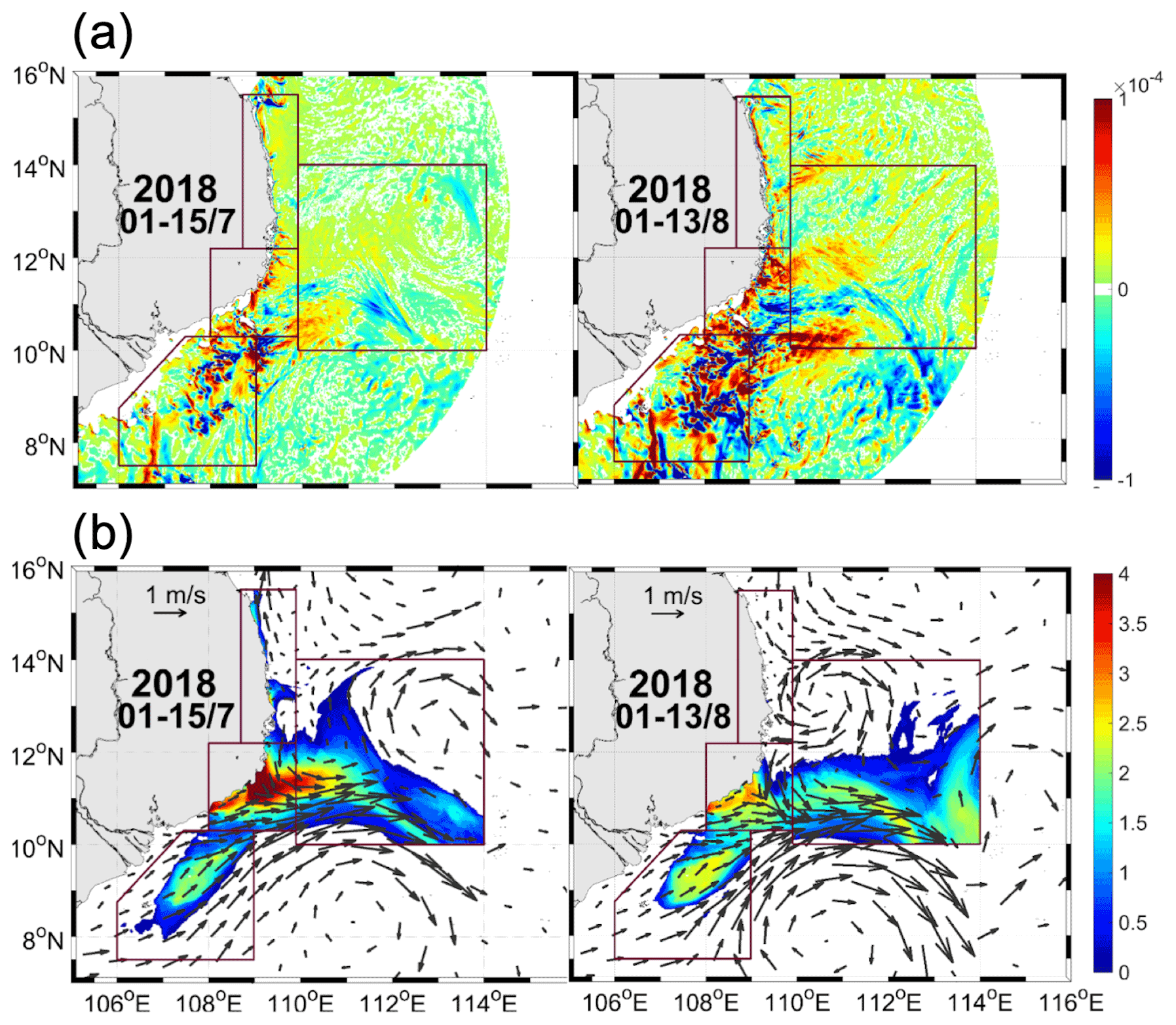
Figure 18Vertical velocity (m s−1, first row) and daily upwelling index (∘C, second row) and surface currents (m s−1) averaged over the July (a, c) and August (b, d) periods of upwelling development in summer 2018.
5.5 Surface cooling over BoxOF: role of offshore upwelling vs. lateral advection of cold water
Most SVU studies assumed that summer surface cooling over BoxOF, which is very similar in OSTIA and SYMPHONIE (Fig. 3), results from of an upwelling developing over BoxOF. However, this surface cooling could also result from the advection by the eastward jet of cold water upwelled at the coast. Three-dimensional simulations can help to answer this question, which cannot be answered from the study of surface variables (temperature, currents) only. Figure 18 shows the maps of the average of simulated vertical velocity at 20 m, the daily upwelling index, and surface currents over the two periods of upwelling development in summer 2018 (summer of the strongest OFU, Fig. 13): the first 2 weeks of July 2018 and the first week of August 2018 (Fig. 15). These figures qualitatively show that BoxOF surface cooling does indeed partly result from the advection of cold water from BoxSC, in particular in July. However, strong upward (positive) vertical velocities are simulated not only along the coast and over BoxMK but also over BoxOF, in particular in August. This confirms that a significant part of surface cooling over BoxOF results from local upwelling. Further dedicated studies, including box analysis following the method used for dense water formation by Herrmann et al. (2008), are now required. They will help to quantitatively assess the respective contributions of lateral advection, surface forcing, vertical advection, and internal mixing to the formation of cold surface water over BoxOF.
The in situ horizontal but also vertical coverage of the region and period of SVU is still very scarce. A high-resolution campaign dedicated to the tridimensional observation of SVU would allow us to evaluate more precisely the capability of the model to reproduce the tridimensional dynamics and water masses but also to better understand the SVU dynamics, including the role of vertical vs. lateral transport of cold water.
The purpose of this study was to simulate the large range of scales of ocean processes and atmospheric forcing, including submesoscale dynamics and high-frequency variability, in order to understand better their role in functioning and variability of the SVU. For that, we implemented a South China Sea configuration of the 3D ocean model SYMPHONIE at high resolution, varying from ∼ 1 km along the Vietnamese coast to ∼ 4 km in the open SCS, and ran a simulation over the period 2009–2018. Comparisons with available satellite data and four sets of in situ observations quantitatively showed the capability of the model to reproduce the ocean circulation and water masses at different scales in the area: from the daily to interannual and climatological scales and from the coastal to offshore regions.
We used this simulation to examine in detail the interannual variability of SVU over three known areas of development: the coastal upwelling that develops along the southern (SCU) and northern (NCU) parts of the Vietnamese coast and the offshore upwelling (OFU). Moreover, our simulation, together with a careful examination of available satellite and in situ data, showed for the first time that upwelling also develops on the Sunda shelf offshore of the Mekong Delta (MKU). Limitations associated with gridded satellite data indeed strongly reduce the spatial observability of small coastal areas, preventing them in particular from capturing the MKU. The high resolution of our simulation allowed us to better capture the SST and current variations over those small coastal areas compared to coarser-resolution numerical outputs and smoothed satellite data. It is therefore a highly valuable tool to complement those observations and examine in detail the functioning and variability of upwelling over its different areas of development.
For SCU and OFU, our results confirmed previous conclusions at the first order: the interannual variability of SCU and OFU intensity is first driven by the intensity of summer wind stress and wind stress curl, which induce Ekman transport and pumping. The intensity of summer circulation in the offshore area (i.e., the ACC dipole and associated eastward jet), also partly induced by the summer wind, also influences this interannual variability. Moreover, the high-resolution of our simulation allowed us to reveal and examine the role of other factors. First, the interannual variability of SCU and OFU intensity is not only influenced by the summer and regional average of the offshore circulation but also by the spatial distribution of (sub)mesoscale and coastal circulation. SCU intensity partly depends on the number and location of ACC dipoles along the coast and on the meridional location of the associated eastward currents. OFU intensity depends on the occurrence, intensity, size, and location of cyclonic eddies north of the eastward jet. Second, our results show that the summer integral of intensity of SCU and OFU is not only driven by the average summer wind but also by its variability at higher frequency. Previous studies already showed the role of wind peaks in the development of OFU and SCU, and we further show here that the timing of those peaks inside the season and inside the month plays an important role. For a given summer average wind intensity, SCU is stronger when wind peaks occur regularly throughout the four JJAS months, compared to situations where peaks occur intermittently during some of the months. In contrast, OFU is strengthened when wind peaks mainly occur during the July–August period, potentially due to a stronger offshore circulation during this period. Moreover, those peaks should be sufficiently spaced to maintain a strong upwelling over a long period. These conclusions should be verified and deepened in dedicated simulations. For NCU, our study confirms that the interannual variability of upwelling intensity is partly driven by the intensity of summer monsoon wind: conditions that favor upwelling in the three other areas prevent NCU. However, we reveal that the role of wind is less important than for the other areas and that the submesoscale to mesoscale circulation that prevails over the coastal area strongly impacts NCU development. NCU is inhibited when alongshore (northward and southward) currents prevail and is enhanced when offshore circulation prevails. Further studies including ensemble simulations are now required to understand which factors, including OIV, favor or prevent the development of these conditions, including of secondary dipoles, along the northern coast.
We showed that MKU develops along the northern flank of the northeastward current in BoxMK, which is part of the wind-induced summer circulation in the offshore region. MKU interannual variability is mostly driven by the interannual variability of this offshore circulation. However, contrary to what is concluded for SCU, OFU, and NCU, MKU is hardly influenced by mesoscale dynamics of a strong chaotic nature, and the spatial structure of currents and upwelling over BoxMK is very stable interannually.
Results presented in this paper therefore allowed us to (1) quantitatively show the quality of a high-resolution model implemented over the Vietnamese coastal area for the study of the SVU and (2) to deepen the existing knowledge about the interannual variability of the SVU over its different areas of development. Sensitivity experiments should now be performed to further explore the different physical processes and scales of variability involved in the SVU, including daily variability of wind and circulation, OIV, rivers, tides, and other non-interannually varying factors. In particular, we did not explore in this paper the mechanisms involved in the development of MKU, but dedicated studies are now required to understand in detail the functioning and variability of this upwelling. Last, this hydrodynamical numerical model is openly available for the scientific community willing to investigate the functioning, variability, and influence of ocean dynamics in the area. It can be used to study other questions related to ocean circulation and dynamics in the region. It can also be coupled with biogeochemical or sediment models (Herrmann et al., 2014, 2017; Ulses et al., 2016) to examine the influence of ocean dynamics on ecosystems and sediment dynamics or used for applied purposes such as pollution monitoring (Estournel et al., 2012; Masumoto et al., 2012; Belharet et al., 2016).
The SYMPHONIE model is available on the web page of the SIROCCO group, https://sirocco.obs-mip.fr/, last access: 25 July 2022 (SImulation Réaliste de l'OCéan COtier, SYMPHONIE developer, Patrick Marsaleix). Outputs of the simulation performed over the period 2009–2018 over the VNC configuration are freely available upon request to the authors.
The supplement related to this article is available online at: https://doi.org/10.5194/os-18-1131-2022-supplement.
TTD, MH, and CE designed the experiments and TTD carried them out, with the support of TD and PM. PM, TD, and CE developed the model code. TTD, NTB, and PM worked on the model optimization. LBH organized the IO-18 survey. TTD and MH prepared the paper with contributions from all co-authors.
The contact author has declared that none of the authors has any competing interests.
Publisher's note: Copernicus Publications remains neutral with regard to jurisdictional claims in published maps and institutional affiliations.
This work is a part of LOTUS international joint laboratory (http://lotus.usth.edu.vn, last access: 25 July 2022). PhD studies of Thai To Duy were funded through an IRD ARTS grant and a “Bourse d'Excellence” from the French Embassy in Vietnam. Numerical simulations were performed using CALMIP HPC facilities (project P13120) and the cluster OCCIGEN from the CINES group (project DARI A0080110098). The IO-18 campaign belongs to the “Study on processes of air–sea–land interactions and environmental variations in Bien Dong in the context of climate change within the framework of IOC\WESTPAC” project; code: DTDL.CN-28/17. This paper is a contribution to celebrate the 100-year anniversary of the Institute of Oceanography, Vietnam Academy of Science and Technology. We warmly thank the two reviewers for the useful and constructive comments that helped improve the quality of the paper.
Glider data were collected by the Vietnam Center for Oceanography (CFO, VASI) in the framework of the USA–Vietnam collaboration project: “Gulf of Tonkin Circulation study” (grant no. NICOP N62909-15-1-2018), financed by the Office of 15 Naval Research (ONR).
This paper was edited by Katsuro Katsumata and reviewed by two anonymous referees.
Ablain, M., Cazenave, A., Larnicol, G., Balmaseda, M., Cipollini, P., Faugère, Y., Fernandes, M. J., Henry, O., Johannessen, J. A., Knudsen, P., Andersen, O., Legeais, J., Meyssignac, B., Picot, N., Roca, M., Rudenko, S., Scharffenberg, M. G., Stammer, D., Timms, G., and Benveniste, J.: Improved sea level record over the satellite altimetry era (1993–2010) from the Climate Change Initiative project, Ocean Sci., 11, 67–82, https://doi.org/10.5194/OS-11-67-2015, 2015.
Belharet, M., Estournel, C., and Charmasson, S.: Ecosystem model-based approach for modeling the dynamics of 137Cs transfer to marine plankton populations: application to the western North Pacific Ocean after the Fukushima nuclear power plant accident, Biogeosciences, 13, 499–516, https://doi.org/10.5194/bg-13-499-2016, 2016.
Bombar, D., Dippner, J. W., Doan, H. N., Ngoc, L. N., Liskow, I., Loick-Wilde, N., and Voss, M.: Sources of new nitrogen in the Vietnamese upwelling region of the South China Sea, J. Geophys. Res.-Ocean., 115, 6018, https://doi.org/10.1029/2008JC005154, 2010.
Boutin, J., Vergely, J. L., Marchand, S., D'Amico, F., Hasson, A., Kolodziejczyk, N., Reul, N., Reverdin, G., and Vialard, J.: New SMOS Sea Surface Salinity with reduced systematic errors and improved variability, Remote Sens. Environ., 214, 115–134, https://doi.org/10.1016/J.RSE.2018.05.022, 2018.
Center for International Earth Science Information Network – CIESIN – Columbia University: Gridded Population of the World, Version 4 (GPWv4), Population Density, Revision 11, https://doi.org/10.7927/H49C6VHW, 2018.
Chao, S. Y., Shaw, P. T., and Wu, S. Y.: El Niño modulation of the South China Sea circulation, Prog. Oceanogr., 38, 51–93, https://doi.org/10.1016/S0079-6611(96)00010-9, 1996.
Chen, C. and Wang, G.: Interannual variability of the eastward current in the western South China Sea associated with the summer Asian monsoon, J. Geophys. Res.-Ocean., 119, 5745–5754, https://doi.org/10.1002/2014JC010309, 2014.
Chen, C., Lai, Z., Beardsley, R. C., Xu, Q., Lin, H., and Viet, N. T.: Current separation and upwelling over the southeast shelf of Vietnam in the South China Sea, J. Geophys. Res.-Ocean., 117, 1–16, https://doi.org/10.1029/2011JC007150, 2012.
Costa, A., Doglioli, A. M., Marsaleix, P., and Petrenko, A. A.: Comparison of in situ microstructure measurements to different turbulence closure schemes in a 3-D numerical ocean circulation model, Ocean Model., 120, 1–17, https://doi.org/10.1016/J.OCEMOD.2017.10.002, 2017.
Da, N. D.: The interannual variability of the South Vietnam Upwelling: contributions of atmospheric, oceanic, hydrologic forcing and the ocean intrinsic variability, PhD thesis, Université de Toulouse, Toulouse, France, 1–168 pp., 2018.
Da, N. D., Herrmann, M., Morrow, R., Niño, F., Huan, N. M., and Trinh, N. Q.: Contributions of Wind, Ocean Intrinsic Variability, and ENSO to the Interannual Variability of the South Vietnam Upwelling: A Modeling Study, J. Geophys. Res.-Ocean., 124, 6545–6574, https://doi.org/10.1029/2018JC014647, 2019.
Damien, P., Bosse, A., Testor, P., Marsaleix, P., and Estournel, C.: Modeling Postconvective Submesoscale Coherent Vortices in the Northwestern Mediterranean Sea, J. Geophys. Res.-Ocean., 122, 9937–9961, https://doi.org/10.1002/2016JC012114, 2017.
Dippner, J. W. and Loick-Wilde, N.: A redefinition of water masses in the Vietnamese upwelling area, J. Mar. Syst., 84, 42–47, https://doi.org/10.1016/J.JMARSYS.2010.08.004, 2011.
Dippner, J. W., Nguyen, K. V., Hein, H., Ohde, T., and Loick, N.: Monsoon-induced upwelling off the Vietnamese coast, Ocean Dynam., 57, 46–62, https://doi.org/10.1007/S10236-006-0091-0, 2007a.
Dippner, J. W., Nguyen, K. V., Hein, H., Ohde, T., and Loick, N.: Monsoon-induced upwelling off the Vietnamese coast, Ocean Dynam., 57, 46–62, https://doi.org/10.1007/s10236-006-0091-0, 2007b.
Estournel, C., Bosc, E., Bocquet, M., Ulses, C., Marsaleix, P., Winiarek, V., Osvath, I., Nguyen, C., Duhaut, T., Lyard, F., Michaud, H., and Auclair, F.: Assessment of the amount of cesium-137 released into the Pacific Ocean after the Fukushima accident and analysis of its dispersion in Japanese coastal waters, J. Geophys. Res.-Ocean., 117, 11014, https://doi.org/10.1029/2012JC007933, 2012.
Estournel, C., Marsaleix, P., and Ulses, C.: A new assessment of the circulation of Atlantic and Intermediate Waters in the Eastern Mediterranean, Prog. Oceanogr., 198, 102673, https://doi.org/10.1016/J.POCEAN.2021.102673, 2021.
Fang, G., Wang, Y., Wei, Z., Fang, Y., Qiao, F., and Hu, X.: Interocean circulation and heat and freshwater budgets of the South China Sea based on a numerical model, Dynam. Atmos. Ocean., 47, 55–72, https://doi.org/10.1016/J.DYNATMOCE.2008.09.003, 2009.
Fang, G., Wang, G., Fang, Y., and Fang, W.: A review on the South China Sea western boundary current, Acta Oceanol. Sin., 31, 1–10, https://doi.org/10.1007/s13131-012-0231-y, 2012.
Fang, W., Fang, G., and Shi, P.: Seasonal structures of upper layer circulation in the southern South China Sea from in situ observations, J. Geophys. Res. Lett., 107, 3202, https://doi.org/10.1029/2002JC001343, 2002.
Gentemann, C. L., Wentz, F. J., Mears, C. A., and Smith, D. K.: In situ validation of Tropical Rainfall Measuring Mission microwave sea surface temperatures, J. Geophys. Res.-Ocean., 109, 4021, https://doi.org/10.1029/2003JC002092, 2004.
Griffies, S. M. and Hallberg, R. W.: Biharmonic Friction with a Smagorinsky-Like Viscosity for Use in Large-Scale Eddy-Permitting Ocean Models, Mon. Weather Rev., 128, 2935–2946, https://doi.org/10.1175/1520-0493(2000)128<2935:BFWASL>2.0.CO;2, 2000.
Herrmann, M., Estournel, C., Déqué, M., Marsaleix, P., Sevault, F., and Somot, S.: Dense water formation in the Gulf of Lions shelf: Impact of atmospheric interannual variability and climate change, Cont. Shelf Res., 28, 2092–2112, https://doi.org/10.1016/J.CSR.2008.03.003, 2008.
Herrmann, M., Estournel, C., Adloff, F., and Diaz, F.: Impact of climate change on the northwestern Mediterranean Sea pelagic planktonic ecosystem and associated carbon cycle, J. Geophys. Res.-Ocean., 119, 5815–5836, https://doi.org/10.1002/2014JC010016, 2014.
Herrmann, M., Auger, P. A., Ulses, C., and Estournel, C.: Long-term monitoring of ocean deep convection using multisensors altimetry and ocean color satellite data, J. Geophys. Res.-Ocean., 122, 1457–1475, https://doi.org/10.1002/2016JC011833, 2017.
Herrmann, M., Ngo-Duc, T., and Trinh-Tuan, L.: Impact of climate change on sea surface wind in Southeast Asia, from climatological average to extreme events: results from a dynamical downscaling, Clim. Dynam., 543, 2101–2134, https://doi.org/10.1007/S00382-019-05103-6, 2020.
Herrmann, M., Nguyen-Duy, T., Ngo-Duc, T., and Tangang, F.: Climate change impact on sea surface winds in Southeast Asia, Int. J. Climatol., 42, 3571–3595, https://doi.org/10.1002/JOC.7433, 2021.
Ho, C. R., Zheng, Q., Soong, Y. S., Kuo, N. J., and Hu, J. H.: Seasonal variability of sea surface height in the South China Sea observed with TOPEX/Poseidon altimeter data, J. Geophys. Res.-Ocean., 105, 13981–13990, https://doi.org/10.1029/2000JC900001, 2000.
Jackett, D. R., McDougall, T. J., Feistel, R., Wright, D. G., and Griffies, S. M.: Algorithms for Density, Potential Temperature, Conservative Temperature, and the Freezing Temperature of Seawater, J. Atmos. Ocean. Technol., 23, 1709–1728, https://doi.org/10.1175/JTECH1946.1, 2006.
Kuo, N. J., Zheng, Q., and Ho, C. R.: Response of Vietnam coastal upwelling to the 1997–1998 ENSO event observed by multisensor data, Remote Sens. Environ., 89, 106–115, https://doi.org/10.1016/j.rse.2003.10.009, 2004.
Large, G. and Yeager, S.: Diurnal to decadal global forcing for ocean and sea-ice models: The data sets and flux climatologies, NCAR/TN-460+STR, University Corporation for Atmospheric Research, https://doi.org/10.5065/D6KK98Q6, 2004.
Leonard, B. P.: A stable and accurate convective modelling procedure based on quadratic upstream interpolation, Comput. Methods Appl. Mech. Eng., 19, 59–98, https://doi.org/10.1016/0045-7825(79)90034-3, 1979.
Li, Y., Han, W., Wilkin, J. L., Zhang, W. G., Arango, H., Zavala-Garay, J., Levin, J., and Castruccio, F. S.: Interannual variability of the surface summertime eastward jet in the South China Sea, J. Geophys. Res.-Ocean., 119, 7205–7228, https://doi.org/10.1002/2014JC010206, 2014.
Li, Y., Han, W., and Zhang, L.: Enhanced Decadal Warming of the Southeast Indian Ocean During the Recent Global Surface Warming Slowdown, Geophys. Res. Lett., 44, 9876–9884, https://doi.org/10.1002/2017GL075050, 2017.
Liu, X., Wang, J., Cheng, X., and Du, Y.: Abnormal upwelling and chlorophyll-a concentration off South Vietnam in summer 2007, J. Geophys. Res.-Ocean., 117, 2–11, https://doi.org/10.1029/2012JC008052, 2012.
Loick, N., Dippner, J., Doan, H. N., Liskow, I., and Voss, M.: Pelagic nitrogen dynamics in the Vietnamese upwelling area according to stable nitrogen and carbon isotope data, Deep-Sea Res. Pt. I, 54, 596–607, https://doi.org/10.1016/j.dsr.2006.12.009, 2007.
Loick-Wilde, N., Bombar, D., Doan, H. N., Nguyen, L. N., Nguyen-Thi, A. M., Voss, M., and Dippner, J. W.: Microplankton biomass and diversity in the Vietnamese upwelling area during SW monsoon under normal conditions and after an ENSO event, Prog. Oceanogr., 153, 1–15, https://doi.org/10.1016/j.pocean.2017.04.007, 2017.
Loisel, H., Vantrepotte, V., Ouillon, S., Ngoc, D. D., Herrmann, M., Tran, V., Mériaux, X., Dessailly, D., Jamet, C., Duhaut, T., Nguyen, H. H., and Van Nguyen, T.: Assessment and analysis of the chlorophyll-a concentration variability over the Vietnamese coastal waters from the MERIS ocean color sensor (2002–2012), Remote Sens. Environ., 190, 217–232, https://doi.org/10.1016/j.rse.2016.12.016, 2017.
Lu, W., Oey, L. Y., Liao, E., Zhuang, W., Yan, X. H., and Jiang, Y.: Physical modulation to the biological productivity in the summer Vietnam upwelling system, Ocean Sci., 14, 1303–1320, https://doi.org/10.5194/OS-14-1303-2018, 2018.
Lyard, F., Lefevre, F., Letellier, T., and Francis, O.: Modelling the global ocean tides: modern insights from FES2004, Ocean Dynam., 565, 394–415, https://doi.org/10.1007/S10236-006-0086-X, 2006.
Marsaleix, P., Auclair, F., and Estournel, C.: Considerations on Open Boundary Conditions for Regional and Coastal Ocean Models, J. Atmos. Ocean. Technol., 23, 1604–1613, https://doi.org/10.1175/JTECH1930.1, 2006.
Marsaleix, P., Auclair, F., Floor, J. W., Herrmann, M. J., Estournel, C., Pairaud, I., and Ulses, C.: Energy conservation issues in sigma-coordinate free-surface ocean models, Ocean Model., 20, 61–89, https://doi.org/10.1016/j.ocemod.2007.07.005, 2008.
Marsaleix, P., Auclair, F., and Estournel, C.: Low-order pressure gradient schemes in sigma coordinate models: The seamount test revisited, Ocean Model., 30, 169–177, https://doi.org/10.1016/j.ocemod.2009.06.011, 2009.
Marsaleix, P., Michaud, H., and Estournel, C.: 3D phase-resolved wave modelling with a non-hydrostatic ocean circulation model, Ocean Model., 136, 28–50, https://doi.org/10.1016/J.OCEMOD.2019.02.002, 2019.
Masumoto, Y., Miyazawa, Y., Tsumune, D., Tsubono, T., Kobayashi, T., Kawamura, H., Estournel, C., Marsaleix, P., Lanerolle, L., Mehra, A., and Garraffo, Z. D.: Oceanic Dispersion Simulations of 137Cs Released from the Fukushima Daiichi Nuclear Power Plant, Elements, 8, 207–212, https://doi.org/10.2113/GSELEMENTS.8.3.207, 2012.
Michaud, H., Marsaleix, P., Leredde, Y., Estournel, C., Bourrin, F., Lyard, F., Mayet, C., and Ardhuin, F.: Three-dimensional modelling of wave-induced current from the surf zone to the inner shelf, Ocean Sci., 8, 657–681, https://doi.org/10.5194/os-8-657-2012, 2012.
Ngo, M. H. and Hsin, Y. C.: Impacts of Wind and Current on the Interannual Variation of the Summertime Upwelling Off Southern Vietnam in the South China Sea, J. Geophys. Res.-Ocean., 126, e2020JC016892, https://doi.org/10.1029/2020JC016892, 2021.
Nguyen-Duy, T., Ayoub, N. K., Marsaleix, P., Toublanc, F., De Mey-Frémaux, P., Piton, V., Herrmann, M., Duhaut, T., Tran, M. C., and Ngo-Duc, T.: Variability of the Red River Plume in the Gulf of Tonkin as Revealed by Numerical Modeling and Clustering Analysis, Front. Mar. Sci., 8, 1636, https://doi.org/10.3389/FMARS.2021.772139, 2021.
Pairaud, I., Lyard, F., Auclair, F., Letellier, T., and Marsaleix, P.: Dynamics of the semi-diurnal and quarter-diurnal internal tides in the Bay of Biscay, Part 1: Barotropic tides, Cont. Shelf Res., 28, 1294–1315, https://doi.org/10.1016/J.CSR.2008.03.004, 2008.
Pairaud, I., Staquet, C., Sommeria, J., and Mahdizadeh, M. M.: Generation of harmonics and sub-harmonics from an internal tide in a uniformly stratified fluid: Numerical and laboratory experiments, in: IUTAM Symposium on Turbulence in the Atmosphere and Oceans, edited by: Dritschel, D., IUTAM Bookseries, Springer, Dordrecht, 28, 51–62, 2010.
Piton, V., Herrmann, M., Marsaleix, P., Duhaut, T., Ngoc, T. B., Tran, M. C., Shearman, K., and Ouillon, S.: Influence of winds, geostrophy and typhoons on the seasonal variability of the circulation in the Gulf of Tonkin: A high-resolution 3D regional modeling study, Reg. Stud. Mar. Sci., 45, 101849, https://doi.org/10.1016/J.RSMA.2021.101849, 2021.
Qu, T.: Upper-Layer Circulation in the South China Sea, J. Phys. Oceanogr., 30, 1450–1460, https://doi.org/10.1175/1520-0485(2000)030<1450:ULCITS>2.0.CO;2, 2000.
Qu, T., Kim, Y. Y., Yaremchuk, M., Tuzuka, T., Ishida, A., and Yamagata, T.: Can Luzon Strait transport play a role in conveying the impact of ENSO to the South China Sea?, J. Clim., 17, 3644–3657, https://doi.org/10.1175/1520-0442(2004)017<3644:CLSTPA>2.0.CO;2, 2004.
Qu, T., Song, Y. T., and Yamagata, T.: An introduction to the South China Sea throughflow: Its dynamics, variability, and application for climate, Dynam. Atmos. Ocean., 47, 3–14, https://doi.org/10.1016/j.dynatmoce.2008.05.001, 2009.
Ray, R. D. and Zaron, E. D.: M2 Internal Tides and Their Observed Wavenumber Spectra from Satellite Altimetry, J. Phys. Oceanogr., 46, 3–22, https://doi.org/10.1175/JPO-D-15-0065.1, 2016.
Reffray, G., Fraunié, P., and Marsaleix, P.: Secondary flows induced by wind forcing in the Rhône region of freshwater influence, Ocean Dynam., 542, 179–196, https://doi.org/10.1007/S10236-003-0079-Y, 2004.
Rogowski, P., Zavala-Garay, J., Shearman, K., Terrill, E., Wilkin, J., and Lam, T. H.: Air-Sea-Land Forcing in the Gulf of Tonkin: Assessing seasonal variability using modern tools, Oceanography, 32, 150–161, https://doi.org/10.5670/OCEANOG.2019.223, 2019.
Sérazin, G., Meyssignac, B., Penduff, T., Terray, L., Barnier, B., and Molines, J. M.: Quantifying uncertainties on regional sea level change induced by multidecadal intrinsic oceanic variability, Geophys. Res. Lett., 43, 8151–8159, https://doi.org/10.1002/2016GL069273, 2016.
Shaw, P. T., Chao, S. Y., and Fu, L. L.: Sea surface height variations in the South China Sea from satellite altimetry, Oceanol. Acta, 22, 1–17, https://doi.org/10.1016/S0399-1784(99)80028-0, 1999.
Siddorn, J. R. and Furner, R.: An analytical stretching function that combines the best attributes of geopotential and terrain-following vertical coordinates, Ocean Model., 66, 1–13, https://doi.org/10.1016/J.OCEMOD.2013.02.001, 2013.
Siew, J. H., Tangang, F. T., and Juneng, L.: Evaluation of CMIP5 coupled atmosphere-ocean general circulation models and projection of the Southeast Asian winter monsoon in the 21st century, Int. J. Climatol., 34, 2872–2884, https://doi.org/10.1002/JOC.3880, 2014.
Toublanc, F., Ayoub, N. K., Lyard, F., Marsaleix, P., and Allain, D. J.: Tidal downscaling from the open ocean to the coast: a new approach applied to the Bay of Biscay, Ocean Model., 124, 16–32, https://doi.org/10.1016/J.OCEMOD.2018.02.001, 2018.
Trinh, B. N.: Cycles de l'eau, de la chaleur et du sel en mer de Chine méridionale, de la variation saisonnière à la variabilité interannuelle: modélisation océanique à haute résolution et à bilan fermé, PhD thesis, Université de Toulouse, Toulouse, France, 2020.
UKMO: GHRSST Level 4 OSTIA Global Foundation Sea Surface Temperature Analysis, https://doi.org/10.5067/GHOST-4FK01, 2005.
Ulses, C., Auger, P. A., Soetaert, K., Marsaleix, P., Diaz, F., Coppola, L., Herrmann, M. J., Kessouri, F., and Estournel, C.: Budget of organic carbon in the North-Western Mediterranean open sea over the period 2004–2008 using 3-D coupled physical-biogeochemical modeling, J. Geophys. Res.-Ocean., 121, 7026–7055, https://doi.org/10.1002/2016JC011818, 2016.
Uu, D. V. and Brankart, J.-M.: Seasonal variation of temperature and salinity fields and water masses in the Bien Dong (South China) sea, Math. Comput. Model., 26, 97–113, https://doi.org/10.1016/S0895-7177(97)00243-4, 1997.
Waldman, R., Somot, S., Herrmann, M., Sevault, F., and Isachsen, P. E.: On the Chaotic Variability of Deep Convection in the Mediterranean Sea, Geophys. Res. Lett., 45, 2433–2443, https://doi.org/10.1002/2017GL076319, 2018.
Wang, B., LinHo, Zhang, Y., and Lu, M. M.: Definition of South China Sea monsoon onset and commencement of the East Asian summer monsoon, J. Clim., 17, 699–710, https://doi.org/10.1175/2932.1, 2004.
Wang, Y., Fang, G., Wei, Z., Qiao, F., and Chen, H.: Interannual variation of the South China Sea circulation and its relation to El Niño, as seen from a variable grid global ocean model, J. Geophys. Res.-Ocean., 111, 1–15, https://doi.org/10.1029/2005JC003269, 2006.
Wang, Y. L. and Wu, C. R.: Nonstationary El Niño teleconnection on the post-summer upwelling off Vietnam, Sci. Rep., 10, 13319, https://doi.org/10.1038/S41598-020-70147-2, 2020.
Woo, H. J. and Park, K. A.: Inter-comparisons of daily sea surface temperatures and in-situ temperatures in the coastal regions, Remote Sens., 12, 1592, https://doi.org/10.3390/RS12101592, 2020.
Wyrtki, K.: Physical oceanography of the South East Asian Waters, Naga Rep., 2, 1–195, 1961.
Xian, W. U., Okumura, Y. M., and Dinezio, P. N.: What controls the duration of El Niño and La Niña events?, J. Clim., 32, 5941–5965, https://doi.org/10.1175/JCLI-D-18-0681.1, 2019.
Xie, S.-P., Xie, Q., and Wang, D.: Summer Upwelling in the South China Sea and its Role in Regional Climate Variations, J. Geophys. Res., 108, 1–37, https://doi.org/10.1029/2003JC001867, 2003.
Xie, S. P., Chang, C. H., Xi, Q., and Wang, D.: Intraseasonal variability in the summer South China Sea: Wind jet, cold filament, and recirculations, J. Geophys. Res.-Ocean., 112, 1–11, https://doi.org/10.1029/2007JC004238, 2007.
Yu, Y., Zhang, H. R., Jin, J., and Wang, Y.: Trends of sea surface temperature and sea surface temperature fronts in the South China Sea during 2003–2017, Acta Oceanol. Sin., 38, 106–115, https://doi.org/10.1007/S13131-019-1416-4, 2019.
Zeng, L., Timothy Liu, W., Xue, H., Xiu, P., and Wang, D.: Freshening in the South China Sea during 2012 revealed by Aquarius and in situ data, J. Geophys. Res.-Ocean., 119, 8296–8314, https://doi.org/10.1002/2014JC010108, 2014.
Zeng, L., Wang, D., Xiu, P., Shu, Y., Wang, Q., and Chen, J.: Decadal variation and trends in subsurface salinity from 1960 to 2012 in the northern South China Sea, Geophys. Res. Lett., 43, 12181–12189, https://doi.org/10.1002/2016GL071439, 2016.
Zeng, L., Chassignet, E. P., Schmitt, R. W., Xu, X., and Wang, D.: Salinification in the South China Sea Since Late 2012: A Reversal of the Freshening Since the 1990s, Geophys. Res. Lett., 45, 2744–2751, https://doi.org/10.1002/2017GL076574, 2018.
Zheng, Z. W., Zheng, Q., Kuo, Y. C., Gopalakrishnan, G., Lee, C. Y., Ho, C. R., Kuo, N. J., and Huang, S. J.: Impacts of coastal upwelling off east Vietnam on the regional winds system: An air-sea-land interaction, Dynam. Atmos. Ocean., 76, 105–115, https://doi.org/10.1016/j.dynatmoce.2016.10.002, 2016.
- Abstract
- Introduction
- Methodology: numerical model and observation datasets
- Model evaluation
- Interannual variability of the South Vietnam Upwelling
- Discussion
- Conclusions
- Code and data availability
- Author contributions
- Competing interests
- Disclaimer
- Acknowledgements
- Financial support
- Review statement
- References
- Supplement