the Creative Commons Attribution 4.0 License.
the Creative Commons Attribution 4.0 License.
 | 28 Jul 2022
Evaluation of basal melting parameterisations using in situ ocean and melting observations from the Amery Ice Shelf, East Antarctica
Madelaine Rosevear
Benjamin Galton-Fenzi
Craig Stevens
Ocean-driven melting of Antarctic ice shelves is causing accelerating loss of grounded ice from the Antarctic continent. However, the ocean processes governing ice shelf melting are not well understood, contributing to uncertainty in projections of Antarctica's contribution to sea level. Here, we analyse oceanographic data and in situ measurements of ice shelf melt collected from an instrumented mooring beneath the centre of the Amery Ice Shelf, East Antarctica. This is the first direct measurement of basal melting from the Amery Ice Shelf and was made through the novel application of an upward-facing acoustic Doppler current profiler (ADCP). ADCP data were also used to map a region of the ice base, revealing a steep topographic feature or “scarp” in the ice with vertical and horizontal scales of ∼ 20 and ∼ 40 m, respectively. The annually averaged ADCP-derived melt rate of 0.51 ± 0.18 m yr−1 is consistent with previous modelling results and glaciological estimates. There is significant seasonal variation around the mean melt rate, with a 40 % increase in melting in May and a 60 % decrease in September. Melting is driven by temperatures ∼ 0.2 ∘C above the local freezing point and background and tidal currents, which have typical speeds of 3.0 and 10.0 cm s−1, respectively. We use the coincident measurements of ice shelf melt and oceanographic forcing to evaluate parameterisations of ice–ocean interactions and find that parameterisations in which there is an explicit dependence of the melt rate on current speed beneath the ice tend to overestimate the local melt rate at AM06 by between 200 % and 400 %, depending on the choice of drag coefficient. A convective parameterisation in which melting is a function of the slope of the ice base is also evaluated and is shown to underpredict melting by 20 % at this site. By combining these new estimates with available observations from other ice shelves, we show that the commonly used current speed-dependent parameterisation overestimates melting at all but the coldest and most energetic cavity conditions.
- Article
(5405 KB) - Full-text XML
- BibTeX
- EndNote


The Antarctic Ice Sheet is losing mass and raising the sea level at an accelerating rate (Bamber et al., 2018; Shepherd et al., 2018; Meredith et al., 2019). This mass loss is due to the acceleration of the glaciers that make up the Antarctic Ice Sheet in response to reduced buttressing by ice shelves (Dupont and Alley, 2005; Fürst et al., 2016; Reese et al., 2018; Meredith et al., 2019), where the reduction in buttressing is driven primarily by increased sub-ice-shelf melting (e.g. Khazendar et al., 2013; Cook et al., 2016; Adusumilli et al., 2018; Minchew et al., 2018). Modelling studies have demonstrated that the grounded ice response to enhanced melting is more sensitive in some areas of the ice shelf, such as grounding zones (Reese et al., 2018). Inter-comparisons of Antarctic Ice Sheet models show that the representation of ocean-induced melting is one of the largest sources of uncertainty in sea level estimates (Seroussi et al., 2020).
Sub-ice-shelf melt rates are controlled by ice–ocean interactions involving a range of temporal and spatial scales (Dinniman et al., 2016) from large-scale circulation to micro-scale ice–ocean boundary layer processes (Gayen et al., 2016; Keitzl et al., 2016; Vreugdenhil and Taylor, 2019). Of critical importance to the magnitude, spatial pattern, and seasonality of the melt rate are the properties of the water masses that intrude into the ice shelf cavity. For example, High-Salinity Shelf Water (HSSW), a cold (T∼ −1.9 ∘C) and dense water mass generated by sea ice formation, tends to drive melting at the back of deep ice shelf cavities. Intrusion of seasonally warmed Antarctic Surface Water (AASW), a much lighter water mass, into cavities drives elevated melt rates in summertime near the ice shelf front (e.g. Arzeno et al., 2014; Stewart et al., 2019). In some locations, relatively warm and salty Circumpolar Deep Water (CDW; T∼ 1 ∘C) accesses ice shelf cavities, where it drives extremely rapid melting (e.g. Cook et al., 2016; Jacobs et al., 2011; Jenkins et al., 2018). CDW-dominated cavities are often termed “warm cavities”, while cavities dominated by HSSW and AASW are known as “cold cavities”. The three largest Antarctic ice shelves – Ross, Filchner–Ronne and Amery – are all cold-cavity ice shelves, and the Amery Ice Shelf is the focus of the present study.
1.1 Amery Ice Shelf
The Amery Ice Shelf (AIS) is an embayed ice shelf in East Antarctica with an area of ∼ 62 000 km2 and some of the deepest Antarctic ice in contact with the ocean (∼ 2200 m; Fricker et al., 2001). Modelling studies suggest that HSSW is present beneath the AIS where it drives moderate melt rates along the eastern flank of the ice shelf cavity (Williams et al., 2001; Galton-Fenzi et al., 2012). The deep draft of the AIS allows HSSW to drive strong melting at the grounding line; a draft of 2200 m depresses the freezing temperature by almost 2 ∘C, resulting in melt rates that exceed 30 m yr−1 (Galton-Fenzi et al., 2012). These elevated melt rates at the grounding line produce cold, fresh, buoyant meltwater called Ice Shelf Water (ISW). ISW ascends the underside of the ice shelf along the western flank of the cavity where it eventually becomes colder than the in situ freezing temperature, allowing frazil ice to form and accumulate on the underside of the ice shelf (Fricker et al., 2001; Herraiz-Borreguero et al., 2013). ISW exits the cavity on the western flank of the AIS at depth, creating a cyclonic circulation within the cavity (Herraiz-Borreguero et al., 2016; Williams et al., 2016).
A sustained observational campaign has improved our understanding of circulation in Prydz Bay and beneath the AIS. The Amery Ice Shelf-Ocean Research (AMISOR) project has been monitoring the ocean beneath the AIS for nearly 2 decades from 2001 on (Allison, 2003). Oceanographic measurements were collected through six boreholes from profiling and the deployment of instrumented moorings for longer-term monitoring (Craven et al., 2004, 2014; Herraiz-Borreguero et al., 2013; Post et al., 2014). These moorings confirmed the presence of both HSSW and ISW beneath the ice shelf. Moorings at the AIS calving front observed a modified version of CDW (mCDW) entering the cavity at intermediate depths during the austral winter (Herraiz-Borreguero et al., 2015), and coincident observations from under-ice mooring AM02 show ISW with a fresher source water mass during this time, suggesting that mCDW drives melting in some areas of the AIS cavity.
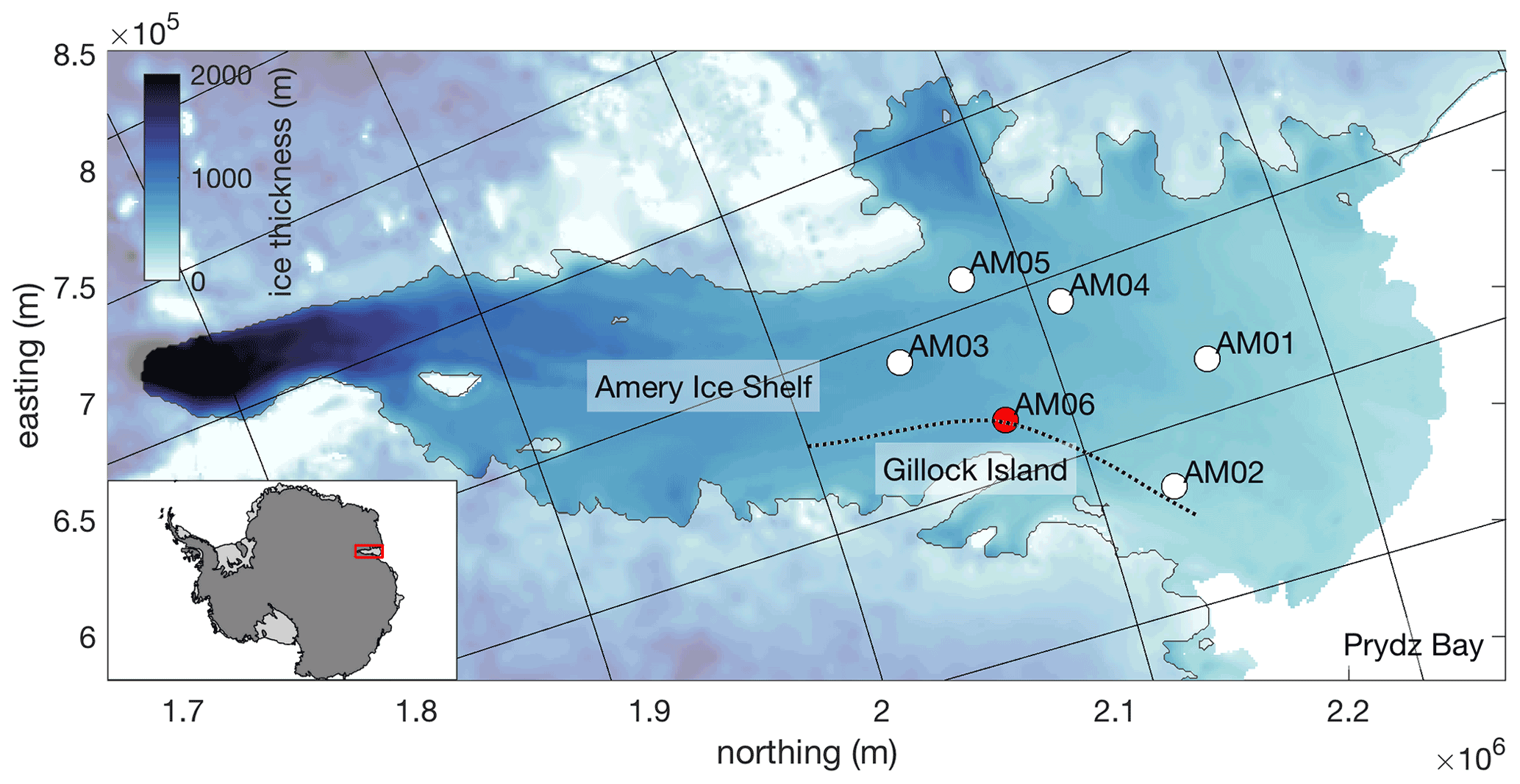
Figure 1Ice thickness map of the Amery Ice Shelf in polar stereographic projection with borehole sites AM01–6 labelled. Site AM06 (magenta) is the focus of this paper. The floating ice shelf is denoted by the bold colours, and the dashed line is the local ice flowline, calculated using the MATLAB flowline function (Greene, 2022) and MEaSUREs ice velocities (Rignot et al., 2017). The map was produced with Antarctic Mapping Tools (Greene et al., 2017) using the Bedmap2 product (Fretwell et al., 2013).
A recent remote sensing study estimated the area-averaged melt rate of the AIS to be 0.8 ± 0.7 m yr−1 over the period 1994–2018 (Adusumilli et al., 2020), consistent with earlier studies (Yu et al., 2010; Wen et al., 2010; Rignot et al., 2013; Depoorter et al., 2013). Modelling and oceanographic studies report similar values of 0.74 m yr−1 (Galton-Fenzi et al., 2012) and 1.0 m yr−1 (Herraiz-Borreguero et al., 2016). Galton-Fenzi et al. (2012) showed a seasonal cycle in area-averaged melt with a maximum of 0.8 m yr−1 in winter and a minimum of 0.7 m yr−1 in summer. The in situ data analysed in the present study were collected at site AM06 (Fig. 1), which is on the eastern flank of the AIS cavity, and are the first such measurements of basal melting from the AIS.
1.2 Melting parameterisation
The ice shelf–ocean boundary layer (ISOBL) regulates heat and salt exchanges between the ice and the far-field ocean and plays a crucial role in determining the rate at which the ice shelf melts. The ISOBL can be broken up into two regions: the diffusive sublayer adjacent to the ice, and the turbulent outer layer. In the narrow diffusive sublayer, the effects of viscosity are dominant and heat and salt are transported by molecular diffusion. The outer layer transport is dominated by turbulent fluxes. The source of this turbulence may be shear instability due to friction between the ocean and ice (e.g. Sirevaag, 2009; Vreugdenhil and Taylor, 2019) or convection due to buoyant meltwater (Kerr and McConnochie, 2015; Keitzl et al., 2016; Gayen et al., 2016; Mondal et al., 2019; Rosevear et al., 2021; Middleton et al., 2021). An extensive review of the roles of current shear and convection in ice–ocean interactions can be found in Malyarenko et al. (2020). Notably, they suggest more work on ice shelf basal roughness at all scales should be a future focus of ice–ocean research. The resolution of general circulation models (e.g. Naughten et al., 2018a) and regional models (e.g. Gwyther et al., 2016; Galton-Fenzi et al., 2012) is far too coarse to capture the ISOBL processes that regulate melting, and a subgrid-scale parameterisation is needed to estimate the melt rate.
Melting is parameterised in these ocean models through a system of equations balancing heat and salt fluxes to the ice–ocean interface with the latent heat and brine fluxes due to melting (e.g. McPhee et al., 1987; Hellmer and Olbers, 1989; Jenkins, 1991; Holland and Jenkins, 1999). Further, it is assumed that the interface temperature (Tb) is at the freezing temperature at interface salinity (Sb) and pressure (pb, Eq. A1 in Appendix A). This results in a system of three equations, which can be solved for Tb, Sb, and melt rate (m). The way in which oceanic heat and salt fluxes are modelled is the key point of difference between melting parameterisations, and we will examine these models next.
1.2.1 Shear-controlled melting
Shear-dependent parameterisations assume the presence of a turbulent boundary layer formed due to friction between the stationary ice and the moving ocean. In this type of parameterisation, oceanic heat and salt fluxes are estimated as a function of friction velocity (u∗, a measure of boundary layer turbulence intensity), the bulk temperature and salinity differences across the boundary layer, and turbulent transfer coefficients for heat (ΓT) and salt (ΓS; Eqs. A2 and A3). It is assumed that this turbulent boundary layer homogenises temperature and salinity below the ice, forming a well-mixed layer, and thus the bulk temperature and salinity differences are expressed as Tb−TML and Sb−SML, where TML and SML are the mixed-layer temperature and salinity, respectively. Friction velocity (u∗) is a function of the stress at the ice–ocean interface – which is unresolved in ocean models – and is typically parameterised as a function of the free-stream current speed (U) and an interfacial drag coefficient (Cd; Eq. A4).
There are several different expressions in the literature for transfer coefficients ΓT and ΓS. Holland and Jenkins (1999), hereafter HJ99, adopt the transfer coefficients of McPhee et al. (1987) for sea ice melting. McPhee et al. (1987) define ΓT and ΓS as functions of flow parameters including the Prandtl (Pr) and Schmidt (Sc) numbers and u∗ (Eqs. A5 and A6), as well as a stability parameter (η), which describes the stabilising effects of meltwater on the flow. HJ99 showed that for Tb−TML < 0.5 ∘C and u∗ > 0.1 cm s−1 (corresponding to U∼ 20 cm s−1) the stability parameter makes less than a 10 % difference on the estimated melt rate. As many of Antarctica's largest ice shelves, such as the Ross, Filchner–Ronne, and Amery, are thought to be relatively cold with strong currents, ocean modellers have typically discounted the effects of stabilising buoyancy by setting η=1 (e.g. Galton-Fenzi et al., 2012; Gwyther et al., 2016; Naughten et al., 2018b).
An alternative parameterisation from Jenkins et al. (2010b), hereafter J10, sets the heat and salt transfer coefficients to observationally derived constants ΓS = 3.1 × 10⁻⁴ and ΓT = 0.011, assuming Cd = 0.0097.
1.2.2 Convection-controlled melting
In the convective melting regime, buoyancy – rather than current shear – is responsible for producing turbulence and setting heat and salt fluxes to the ice. Recent laboratory (McConnochie and Kerr, 2016), turbulence-resolving numerical (Gayen et al., 2016; Mondal et al., 2019) and theoretical (Kerr and McConnochie, 2015) studies have focused on this regime in which melting of a sloping or vertical ice boundary is controlled by temperature and does not depend directly on current speed. For a sloping ice–ocean interface McConnochie and Kerr (2018), hereafter MK18, show that m scales as , where T∞ is the far-field ocean temperature, and scales with the basal slope (θ) as (Eqs. A7 and A8). An equivalent expression was determined using turbulence-resolving numerical simulations (Mondal et al., 2019).
A transition from convective to shear-driven melting is expected as flow speeds increase near the ice (McConnochie and Kerr, 2017b). Wells and Worster (2008) proposed a transition based on a critical Reynolds number for the diffusive sublayer (Reδ). These criteria were applied to observational data by Malyarenko et al. (2020), who found that a shear parameterisation tended to reproduce observed melt rates well above a threshold of Reδ∼ 20.
1.3 Present study
This study presents a set of in situ oceanographic and basal melting observations collected beneath the AIS in 2010. Using this unique dataset, we will seek to address these questions: (i) what is the ocean variability in the AIS cavity; (ii) how does this relate to measured melt rate in terms of mean and variation; (iii) how well do available parameterisations predict the basal melt rate in this situation, and (iv) how do these data compare to other published datasets of concurrent melt rate and ocean observations?
2.1 AM06 borehole and instrumentation
The borehole at AM06 (70∘14.7′ S, 71∘28.1′ E) was hot-water drilled during the 2009/2010 summer at a site that was predicted to be melting (Galton-Fenzi et al., 2012). The ice shelf at this location is 607 m thick, with 73 ± 2 m of freeboard, and the water column thickness is 295 m. The ice–ocean interface and seafloor are at 523 ± 2 and 837 ± 2 dbar, respectively.
Several conductivity–temperature–depth (CTD) casts were collected over the full depth of the cavity during a 2 d period using a Falmouth Scientific Instruments (FSI) 3′′ Micro CTD instrument (serial 1610). Pre-season laboratory calibrations of the FSI CTD temperature, pressure, and conductivity sensors were done at the Commonwealth Scientific and Industrial Research Organisation Division of Marine Research; however, no in situ calibrations were performed. Based upon the largest corrections from previous AMISOR sites (using the same instrument) the error is expected to be less than 0.005 ∘C, 0.3 psu, and 3 dbar for temperature, salinity, and pressure, respectively. A mooring, comprising three Seabird SBE37IM MicroCATs and one upward-looking RDI 300 kHz Workhorse acoustic Doppler current profiler (ADCP), was then deployed through the ice. Weights were affixed to the end of the mooring to apply tension to the cable and minimise motion of the instruments. All instruments sampled at 30 min intervals. In the vertical, the ADCP sampled 27 bins at 4 m resolution, where 23 of the bins were within the water column. The beam angles were 20∘ from the vertical. The location of each instrument with respect to the ice–ocean interface is outlined in Table 1. The duration of the ADCP record is 366 d, and thus we restrict the analysis of the MicroCAT data to the same period for this study. In situ temperature (T) and practical salinity (S) are converted to conservative temperature (Θ) and absolute salinity (SA) using the Gibbs Seawater MATLAB package (McDougall and Barker, 2011).
Table 1Type, duration and depth of measurements from the AM06 borehole. Depth given with respect to the ice–ocean interface on 1 January 2010.

2.2 ADCP-derived ice morphology and melting
The range from the ADCP to the ice shelf is used to map the ice shelf base and measure the local melt rate. To our knowledge, ours is the first study to use an ADCP in this manner beneath an ice shelf. To map the ice shelf base we use the bottom tracking functionality of the ADCP. A range measurement is obtained from each of the four ADCP beams, which are oriented at 20∘ to the vertical and at 90∘ to each other, and the range, heading, pitch, and roll data are used to map the interface position in x, y, and z. The instrument rotates about the mooring line due to tidal currents, allowing the ADCP beams to map out a circular swath of the underside of the ice. We find that the bottom tracking data are too noisy to recover a direct melt rate measurement. Instead, for the melt rate estimates, range is obtained by post-processing the echo amplitude (intensity) of the ADCP pings. Following the method outlined in Shcherbina et al. (2005), a modified Gaussian is used to approximate the surface reflection peak profile A(z):
where a0, a1, a2, h0, and δ are obtained by a least-squares fit of Eq. (1) to the echo amplitude data in the vicinity of the surface peak. The fitted value of h0 is an estimate of the range from the ADCP to the ice shelf.
The fit is found for each of the four ADCP beams independently. Ideally, an average over the four beams would be used to decrease the statistical error (Shcherbina et al., 2005). However, this was not possible due to the shape of the ice shelf base (in Sect. 3 we will show that the ice shelf draft changes by 20 m over a horizontal distance of only 40 m). All four ADCP beams are mapped to polar coordinates and binned in dϕ × dr = 4∘ × 3 m bins. While the ADCP samples at 30 min intervals, the sampling frequency for each bin is variable, as it depends on the rotation of the ADCP about the mooring line due to currents. In practice, some areas of the ice base are frequently sampled and others rarely. If a bin has > 5 range estimates in a month-long period, an average ice–ocean interface depth is returned (e.g Fig. B1 in Appendix B). Melt rates are calculated from a centred finite difference of the interface depth. Unfortunately, the surface reflection peak in Eq. (1) is not captured for ice ≳100 m from the ADCP. This constraint, combined with spatially and temporally inconsistent sampling, means that the depth of the interface can only be calculated using this method for headings , and consequently melt rate estimates are limited to this area.
Our methods of determining the position of the ice–ocean interface (and melting) are sensitive to motion of the ADCP; we assume that the ADCP remains fixed in space (in a frame of reference moving with the ice shelf) in order to transform the range, heading, pitch, and roll measurements into an interface position in x, y and z. Fortunately, the pressure sensor of the middle MicroCAT (mCAT2), 40 m below the ADCP shows that the motion of the ADCP was relatively small. The maximum pressure anomaly is −0.9 dbar (associated with a vertical excursion of < 1 m), and excursions were typically much smaller than this. In order to avoid contamination of the interface position and melt rate measurements by this motion, we have excluded data when the pressure anomaly at mCAT2 is < −0.25 dbar, corresponding to < 2 % of data.
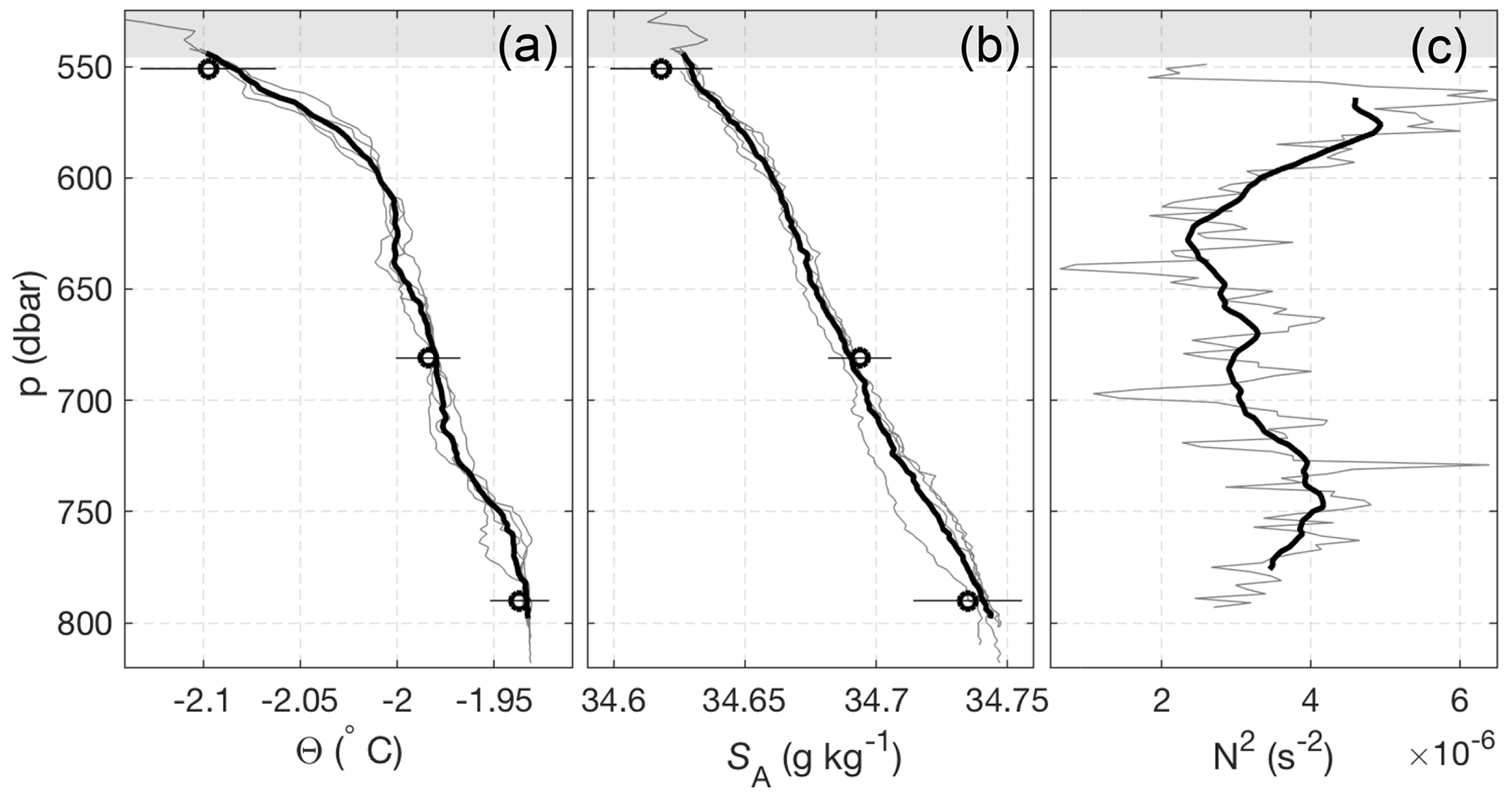
Figure 2(a) Conservative temperature (Θ) and (b) Absolute salinity (SA) profiles from the two CTD casts at AM06. Individual up and down casts are shown (grey lines), with the four-profile mean also shown (black line). Overlain at the appropriate pressures are the mean (± 2σ) MicroCAT Θ and SA for the month following the CTD data collection. (c) Squared buoyancy frequency (N2) profiles, where the grey and black buoyancy frequency curves were obtained using 10 and 40 dbar running window averages, respectively. The shaded grey region shows range in the ice–ocean interface position above the instruments due to the sloping ice base.
3.1 Water column structure
CTD casts collected before the deployment of the mooring at AM06 show a water column stratified in both temperature and salinity, with cooler, fresher water overlying warmer, saltier water (Fig. 2). There is no systematic difference between the up and down casts of the CTD, and we include both here. The water column is stably stratified with depth-mean stratification N2∼ 3.5 × 10⁻⁶ s−2, where is the buoyancy frequency. There is no mixed layer beneath the ice, and the temperature gradient is especially strong in the upper 30 m of the water column. There is some evidence for a benthic mixed layer below ∼ 790 dbar, although this was not consistently sampled by the CTD.
Figure 3 shows the four-cast mean Θ−SA properties from the CTD. A defining feature of ocean conditions beneath ice shelves is the presence of meltwater from meteoric (fresh) ice, which causes ocean properties to evolve along nearly straight line in Θ−SA space (e.g. Gade, 1979; Hattermann et al., 2012; Stevens et al., 2020). Under the assumption of equal eddy diffusivities for heat and salt, the gradient () of this “meltwater mixing line” can be calculated (Gade, 1979; McDougall et al., 2014). At local conditions Eq. (16) of McDougall et al. (2014) gives = 2.38 C g−1 kg, and explains the Θ−SA properties well over the pressure range 560–620 dbar. Below 620 dbar, temperatures remain below the surface freezing temperature; however, Θ−SA properties do not follow a meltwater mixing line, suggesting mixing between two different meltwater-modified water masses. Below 750 dbar, the HSSW observed is essentially unmodified. Near the interface, the gradient steepens, deviating from the meltwater mixing line. A line of best fit over this 15 m thick layer has slope = 4.8 C g−1 kg. This implies that the turbulent diffusivities of heat and salt are not equal over this region. Stratification can alter the ratio of turbulent diffusivities (Jackson and Rehmann, 2014); however, stratified turbulence effects would be expected to decrease the gradient. The steep gradient could instead be indicative of diffusive convection, which is known to occur beneath ice shelves due to the presence of cold, fresh meltwater at the ice–ocean interface. The ratio describes the stability of a system to diffusive convection, where observations suggest that the water column is susceptible to diffusive convection for , with stronger convection as Rρ approaches 1 (Kelley et al., 2003). Using α = 3.8 × 10⁻⁵ () and β = 7.8 × 10⁻⁴ (g kg−1), we find Rρ = 4.3, indicating that the system is susceptible to diffusive convection. However, we note this value is high compared to the Rρ = 2 observed beneath George VI Ice Shelf, where diffusive convection was observed (Kimura et al., 2015).
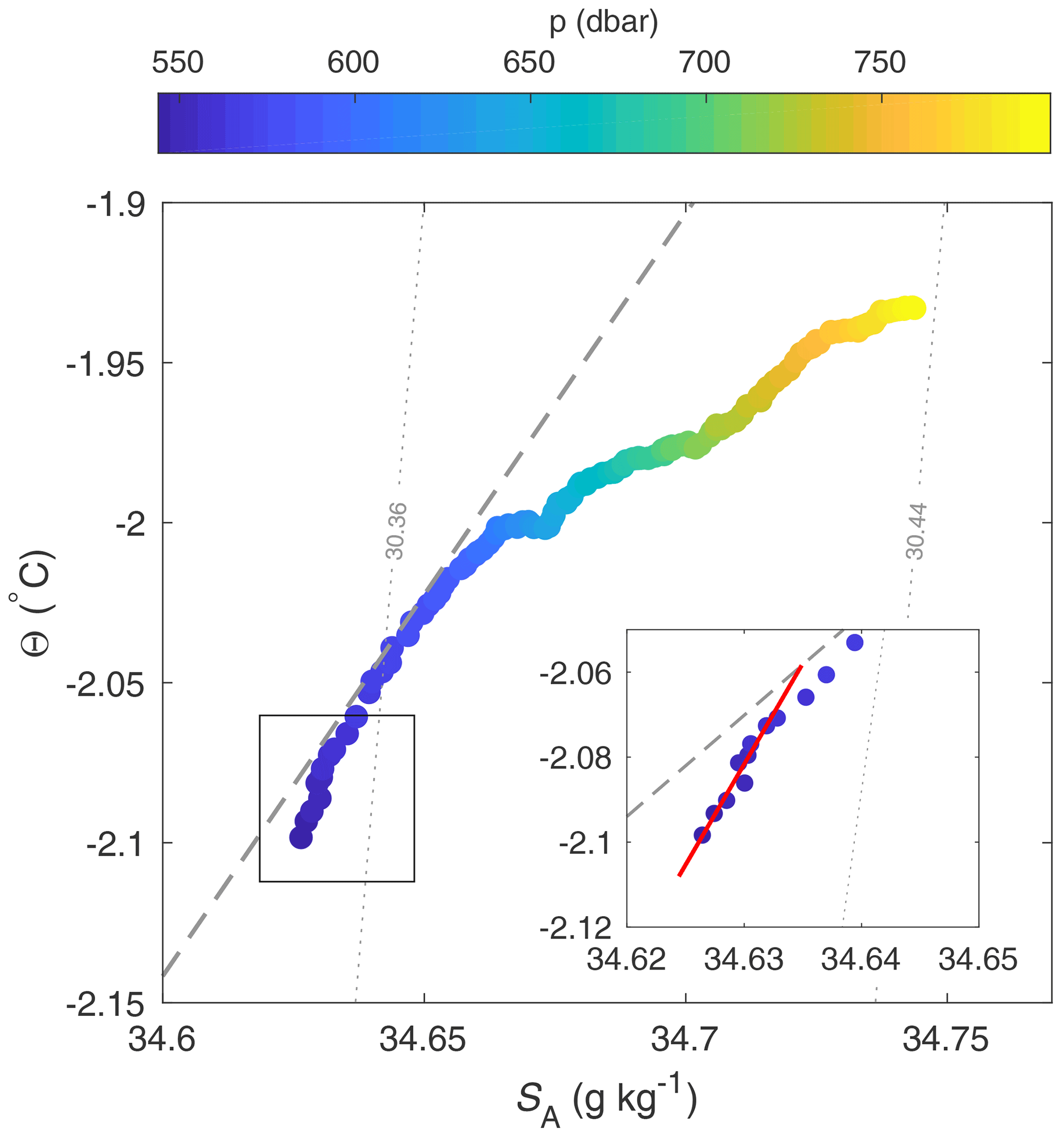
Figure 3Θ–SA plot of the four-profile mean from Fig. 2 coloured by pressure. A meltwater mixing line with gradient = 2.38 calculated following McDougall et al. (2014) is shown (dashed grey line) alongside the local isopycnal slopes (dotted grey lines). The inset shows a line of best fit for the upper 15 m of the water column (red line), which has gradient = 4.8 .
The time series of temperature and salinity measurements from the upper water column indicate that AM06 is a site of melting year-round. For the whole period sampled, the temperature recorded by the upper MicroCAT is greater than the in situ freezing temperature at the interface pressure (543 dbar) by ∼ 0.2 ∘C (Fig. 4). Temperatures recorded at all depths are colder than the surface freezing temperature (−1.9 ∘C), indicating the presence of ISW, and show similar seasonality at all depths (Fig. 4). The water column, which is warmest in summer and autumn, cools over winter and reaches a minimum temperature in spring. The cooling is coincident with freshening at all depths. In October, the cooling and freshening trend reverses and temperature and salinity increase rapidly towards their previous summer values.
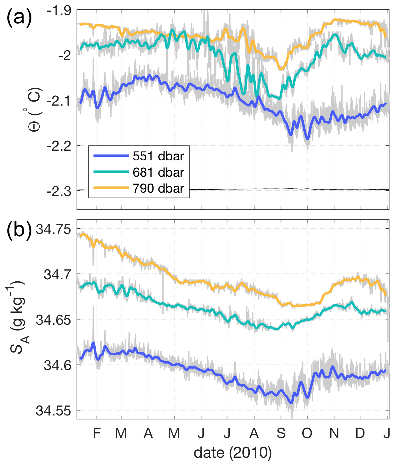
Figure 4Time series of (a) Θ and (b) SA from all three MicroCATs. Bold lines are smoothed at 1 week, while grey lines are not smoothed. The freezing temperature (black) at upper MicroCAT salinity and interface pressure is also shown in (a).
MicroCAT temperatures and salinities fall on a melt-freeze line (McDougall et al., 2014), demonstrating that the water masses arriving at AM06 have been modified by the addition of fresh water due to ice melt, with the highest fraction of meltwater at the MicroCAT nearest the ice base. The ISW present at AM06 follows a single melt–freeze line year round (Fig. 5), suggesting a single ISW source water mass with SA∼ 34.68 g kg−1. Whilst it is not possible to use the melt–freeze relationship to unequivocally identify the source water masses of the ISW, the high salinity suggests that it is HSSW driving melt at AM06, where we follow Herraiz-Borreguero et al. (2015) in defining HSSW as having −1.85 −1.95 and SA > 34.67 g kg−1. The Θ−SA minimum in spring is likely the result of a high degree of modification of HSSW by meltwater (Fig. 5).
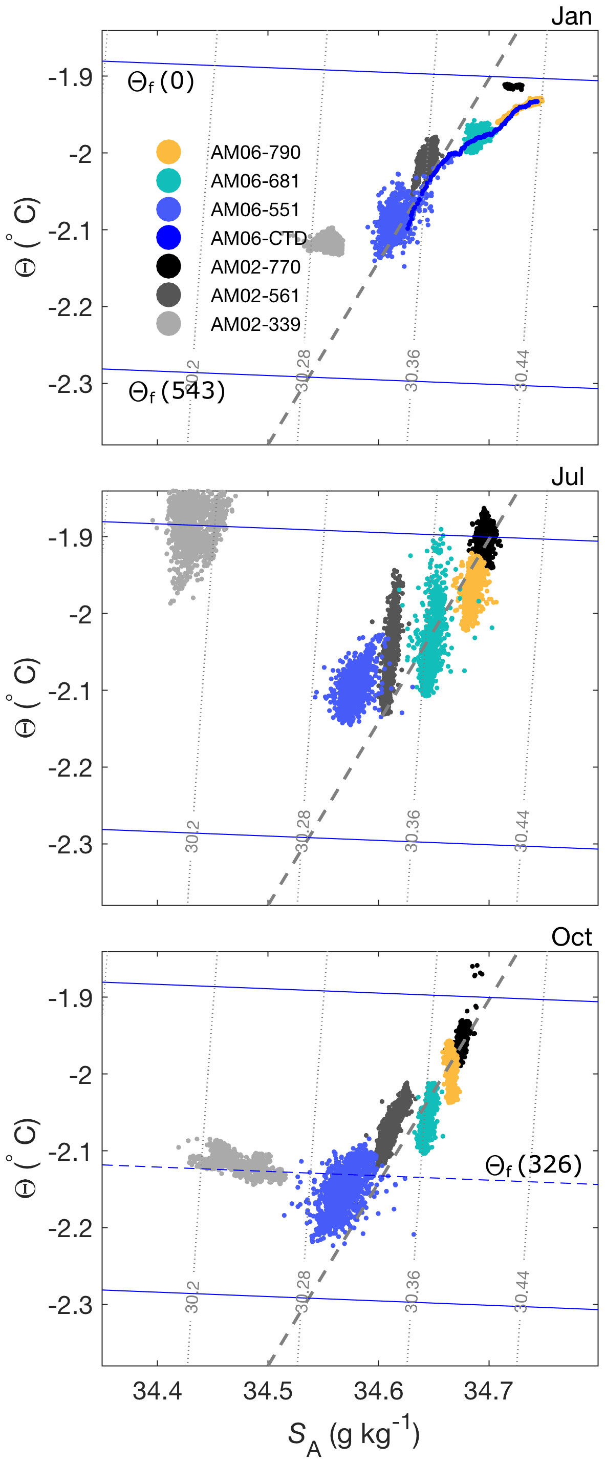
Figure 5Θ–SA plots for January, July, and October of AM06 (2010) and AM02 (5 year composite of years 2001, 2003–2006). Freezing temperature curves at the surface (0 dbar), AM06 interface (543 dbar), and AM02 interface (326 dbar, bottom panel only) pressure are also shown. The dashed grey line is the meltwater mixing line from Fig. 3.
A multi-year composite of Θ−SA from mooring AM02 (Herraiz-Borreguero et al., 2015), situated midway (∼ 70 km) from AM06 to the calving front and spanning the years 2001 and 2003–2006, is also shown in Fig. 5. The data from AM02 MicroCATs at 561 and 770 dbar show similar seasonality and properties to AM06. At these depths, Θ−SA properties at the two mooring locations follow the same meltwater mixing line, suggesting the same source water mass, although the ocean is typically cooler and fresher at AM06 than at AM02 at an equivalent depth. This could imply a circulation from AM02 to AM06, with meltwater accumulating as the water mass moves deeper within the cavity. However, the warmer mCDW observed at AM02 at 339 dbar in July (Herraiz-Borreguero et al., 2015) is not observed at AM06, likely due to the deeper ice shelf draft at AM06. In October, a water mass at the local freezing temperature with a range of salinities is observed at AM02 at the 339 dbar MicroCAT. This water mass is likely the result of a rising meltwater plume raised to the in situ freezing point by frazil ice formation (e.g. Stevens et al., 2020).
3.2 Currents
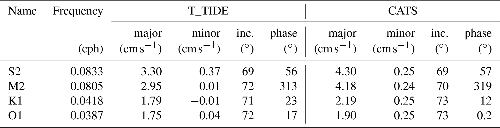
Currents at AM06 have speeds on the order of 10 cm s−1 and consist of both tidal and mean components (Fig. 6). To determine the dominant tidal constituents we perform a harmonic analysis of the depth-mean currents using the T_TIDE package (Pawlowicz et al., 2002), restricting the analysis to frequencies higher than semi-annual due to the limited duration of the ADCP record. The analysis shows that the tides have mixed semidiurnal and diurnal properties. The ellipse semi-major velocities of semidiurnal constituents S2 and M2 are 3.3 and 3.0 cm s−1, respectively, which is larger than those of diurnal constituents K1 and O1, which are 1.9 and 1.8 cm s−1, respectively (Table 2). Ellipse semi-minor velocities for both diurnal and semidiurnal constituents are small, indicating that tides are close to rectilinear. Tides are oriented NNE–SSW, roughly normal to the AIS calving front. At AM06 the CATS2008 circum-Antarctic tide model (an update to the model described in Padman et al., 2002) performs relatively well against the T_TIDE fits, although the CATS estimates are ≲ 25 % higher across the constituents examined (Table 2). This could be due to errors in the bathymetry used in CATS, as tide modelling is sensitive to water column thickness and bathymetry is typically poorly constrained beneath ice shelves. In light of this, the CATS model performs remarkably well at AM06. Our observations of mixed semidiurnal–diurnal tidal currents are similar to previous results from barotropic tidal modelling, which showed magnitudes of ∼ 5 and ≲ 2 cm s−1 for the semidiurnal and diurnal tides, respectively (Hemer et al., 2006).

Figure 6(a) Depth-mean current speed from 19–91 m below the ice (grey). Overlaid is the smoothed residual current speed (Ur, blue). (b) Current direction from north (grey) and smoothed residual current direction (red). (c) Monthly mean (〈U〉) and root-mean-square (rms (U)) current speed for depth ranges 7–19 and 19–91 m below the ice. Current speed data over the depth range 7–19 m is not plotted for the months January–April due to poor data return near the ice during that period.
An estimate of the typical tidal current magnitude is given by
where ue and ve are the magnitudes of the semi-major and semi-minor axes of the tidal ellipse, with subscript i representing the four main tidal constituents. Utyp is roughly the maximum current speed available from these four constituents. Using the constituents in Table 2 yields Utyp=9.8 cm s−1 at AM06. Instantaneous current speeds at AM06 in excess of 15 cm s−1 (Fig. 6) are a consequence of the superposition of mean and tidal currents.
Table 2Ellipse parameters for tidal current constituents of the depth-mean flow over the upper 90 m of the water column from the T_TIDE harmonic analysis (Pawlowicz et al., 2002) and predicted by the CATS2008 tidal model. The parameters are velocities of the ellipse major and minor axes, inclination of the semi-major axis (counter-clockwise from east), and phase of the tidal vector relative to equilibrium tide at Greenwich.
In order to consider the tidal and non-tidal currents separately, we remove the best-fit T_TIDE tidal velocities (uT, vT) from the observed depth-mean velocities, yielding the residual flow . Figure 6 compares the total and residual flow speeds, where the residual flow is smoothed with a Gaussian filter with a half-width of 1 week. The residual flow is oriented into the cavity (220∘ N), has an annual mean speed of 3.2 cm s−1, and varies seasonally and at higher frequencies. Notably, in the period August–December Ur is at its weakest and the water column is cold and fresh (Fig. 4), suggesting increased residence time beneath the ice resulting in a higher meltwater fraction at this time. We also compare the monthly mean and root-mean-squared currents near the ice (U7–19) and deeper in the water column (U19–91), where near-ice currents are not shown prior to April due to poor data return near the ice in this period (Fig. 6c). We find that near-ice current speeds are typically weaker than deeper currents, excepting October–November period when currents are surface-intensified.
3.3 AIS cavity circulation
The conditions observed beneath the AIS are qualitatively similar to conditions observed in other large cold-type ice shelf cavities, the Ross and Filchner–Ronne ice shelves, where the water column away from the ice shelf front is dominated by cold ISW (e.g. Nicholls et al., 2004; Stevens et al., 2020). The AIS is the only one of these three ice shelf cavities within which mCDW has been observed (Herraiz-Borreguero et al., 2015). However, the mCDW observed entering the AIS cavity has been heavily modified and is much colder (T≲ −1.6 ∘C) than the CDW in intruding beneath rapidly melting ice shelves such as Pine Island Ice Shelf (T∼ 1.0 ∘C, Jenkins et al., 2010a). The mCDW was not observed at site AM06; however, the depth of the ice at AM06 (∼ 600 m) is likely to exclude mCDW, which only occupies depths ≳ 600 m at the calving front (Herraiz-Borreguero et al., 2016).
Our observation from site AM06 of HSSW-derived ISW with a mean flow of ∼ 3.0 cm s−1 oriented into the cavity supports a three-dimensional model of AIS cavity circulation, consistent with observations from other AIS moorings (Herraiz-Borreguero et al., 2013, 2015) and modelling results (Galton-Fenzi, 2009). These earlier studies suggested a pathway for HSSW from the calving front into the AIS cavity past AM02 and AM06, which are situated on the eastern flank. The HSSW cools and freshens due to basal melting, with a return flow on the western flank of the ice shelf driven by a buoyant ISW plume.
3.4 ADCP-derived basal melt rate
The ADCP-based estimate of the annual mean melt rate at AM06 is 0.51 ± 0.18 m yr−1 (Fig. 8). Monthly averaged melt rates range from a maximum of 0.8 m yr−1 in May to a minimum of 0.2 m yr−1 in August and September. The seasonality in melting is consistent with the seasonality of upper MicroCAT temperatures. Broadly speaking, when temperatures are warmer, higher melt rates are observed (Fig. 4). However, the period of maximum melt in June does not coincide with the warmest ocean temperatures, which are observed in April for the upper MicroCAT. Mean and root-mean-squared currents are slightly reduced in the period August–November, coincident with the period of low melt rates (Fig. 6).
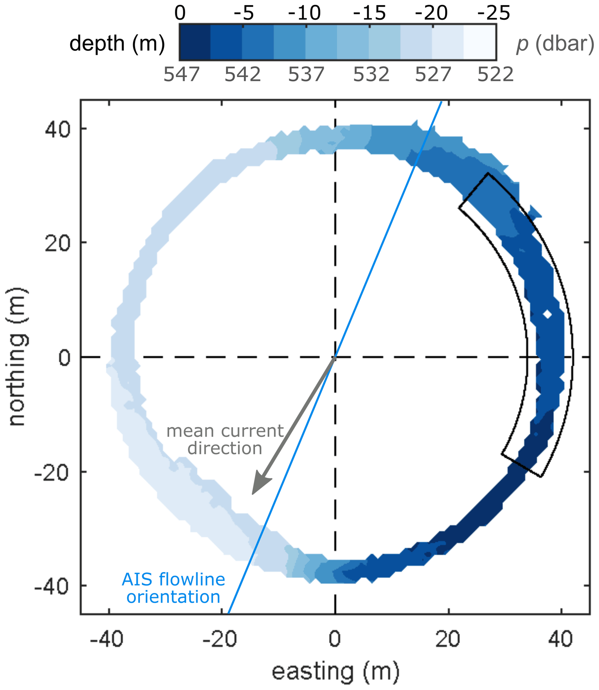
Figure 7The ice shelf base as seen by the upward-looking ADCP. Zero depth is defined at p = 547 dbar, the deepest ice measured at the site, and a negative depth indicates shallower ice. The area mapped out by the ADCP is determined by the beam angle (20∘) and the distance to the ice shelf (92–114 m). The full year of data are binned into 1 m × 1 m bins and averaged to produce this figure, where a typical standard deviation for a bin is 1.3 m. Overlain is an outline of the region of the ice base over which melt rates in Fig. 8 are calculated. The local ice shelf flowline orientation and direction of the mean current observed at AM06 are also indicated.
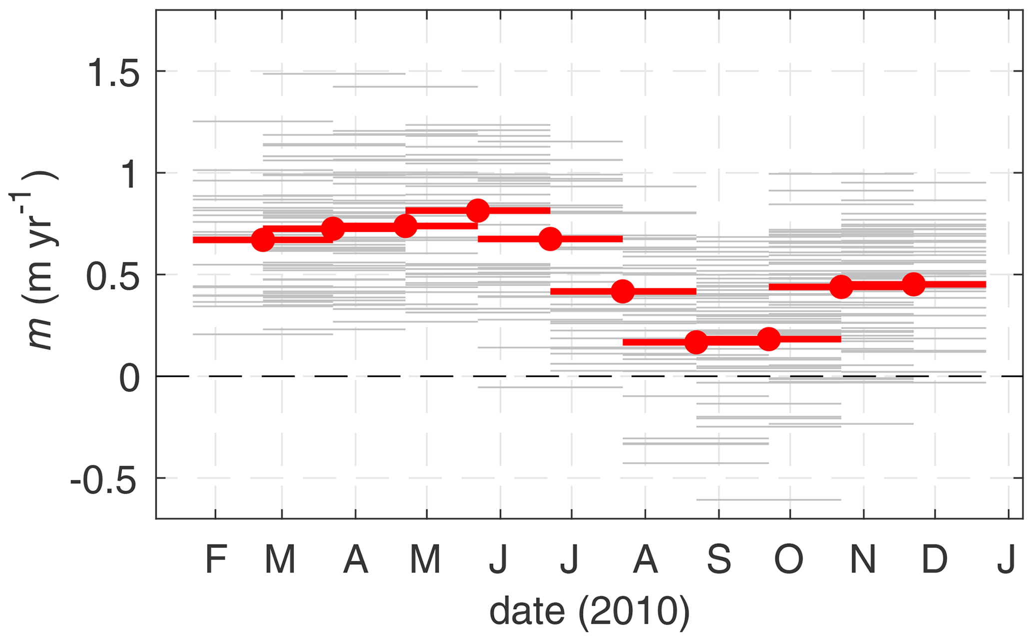
Figure 8Observed melt rates from the ADCP at monthly resolution for (grey) each bin (dϕ, dr) and (red) the area average, where the area is outlined in Fig. 7. Melt rates are calculated from interface depth using centred differences (i.e. .
The melt rate measured here in situ is consistent with the modelled melt rate in the vicinity of AM06 (∼ 1 m yr−1; Galton-Fenzi et al., 2012), and more broadly with AIS area-averaged melt rates from models (0.74 m yr−1; Galton-Fenzi et al., 2012), oceanographic proxies (1.0 m yr−1; Herraiz-Borreguero et al., 2016), and glaciological studies (0.5–0.8 m yr−1; Yu et al., 2010; Wen et al., 2010; Rignot et al., 2013; Depoorter et al., 2013; Adusumilli et al., 2020). However, the seasonal cycle in melting at AM06 is somewhat out of phase with the modelled cavity average, which has a maximum in July and a minimum in January (Galton-Fenzi et al., 2012).
3.5 ADCP-derived basal morphology
Data from the ADCP bottom tracking function reveals a large topographic feature or “scarp” in the underside of the ice shelf at AM06 (Fig. 7). The scarp has a vertical extent of ∼ 20 m and a maximum slope of 45∘. The along-scarp direction is roughly north–south, and the ice deepens moving from east to west. The mean current direction (220∘ N) is neither along-scarp, as may be expected if the basal topography was playing an important role in guiding the flow, nor cross-scarp, which could result in flow acceleration, separation, and/or blocking. This scarp is an interesting and unexpected feature of the site. There are very few surveys of shelf undersides at the 1–100 m scale due to difficulty of access. Consequently, the ice base is typically assumed to be smooth, at least at small scales. However, our observation of steep topography with vertical and horizontal scales of ∼ 20 and ∼ 40 m, respectively, adds to the small but growing number of studies demonstrating that the underside of ice shelves are not necessarily smooth and may exhibit “roughness” at the O(10 m) scale (Nicholls et al., 2006; Dutrieux et al., 2014).
The limited spatial coverage of the ADCP makes is difficult to draw conclusions about the nature or origin of our “scarp”; however, we present several possibilities. For example, the scarp may be an isolated feature, one element of a “rough” patch of ice (Nicholls et al., 2006) or part of a larger system, for example, a terrace on the flank of a basal channel (Dutrieux et al., 2014) or a suture zone with its origin upstream. A thorough investigation of the glaciological origins of this scarp is outside the scope of the present study; however, we note that the scarp is not closely aligned with the local ice flowline (Fig. 7), as would be expected if the scarp was suture zone between two ice tributaries of different thickness, nor does it have a surface expression consistent with a larger channel system. The scarp could also be formed by ocean processes: for example, a convective process known as double-diffusive convection can drive differential melting of a vertical ice face (Huppert and Turner, 1978). Evidence of double-diffusive convection has been seen in observations and models of the ocean beneath ice shelves (Kimura et al., 2015; Middleton et al., 2021; Rosevear et al., 2021); however, it is likely that the currents at AM06 are too strong for this process to dominate circulation near the ice and produce such a significant feature through differential melting.
There are many other possible feedbacks between complex topography, flow, and melting. For example, acceleration of buoyant flow up slope, higher melting on steep slopes (McConnochie and Kerr, 2017b), and differential effects of stratification on melting for flat vs. sloping ice (Vreugdenhil and Taylor, 2019; McConnochie and Kerr, 2016) are all possible. Due to the background currents, phenomena such as flow blocking, acceleration, and separation can also be expected, depending on ocean stratification and the orientation of the flow with respect to the scarp. These effects will be maximised when the flow is across-scarp; however, flow at AM06 is primarily along-scarp (Fig. 7). The effects of basal topography on flow and melting warrant further investigation using field measurements of velocity at high resolution (e.g. sub-metre) and complementary modelling studies.
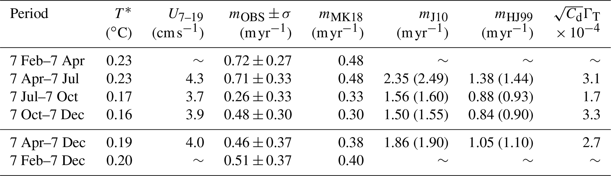
Table 3Melt rates from observations and parameterisations. Columns 2–4 are average values observed over the periods given in column 1. Current speed U is depth-averaged over 7–19 m below the ice base. To calculate mHJ99 a drag coefficient of Cd = 0.0025 is used. The bracketed melt rate estimates show the effect of setting the heat flux into the ice shelf to zero. The final column is the best-fit Stanton number .
4.1 Choice of data
Here we use the concurrent temperature, salinity, and velocity measurements from site AM06 to predict the local melt rate using three different melt rate parameterisations. We test two current shear-dependent parameterisations solving Eqs. (A1)–(A3), one with the constant transfer coefficients recommended in J10 and the other using Eqs. (A5) and (A6) from HJ99. We also test the convective parameterisation solving Eqs. (A1), (A7) and (A8) from MK18. Because the ADCP-derived melt rate estimates are relatively noisy, we consider averages over 2–3-month periods when comparing observed and parameterised melt rates (Table 3). This reduces uncertainty in the observed melt rates, while retaining some of the observed seasonal variability. The mixed-layer temperature (TML) and salinity (SML) are taken from the upper MicroCAT. Because of the sloped ice–ocean interface, the positioning of this instrument with respect to the ice depends on the region of ice considered. Here we use the lower bound on the interface position (z = −541 m) as our reference depth. The upper MicroCAT is therefore situated at a depth of 4 m (Table 1). Choosing the upper bound (z = −519 m) would put the upper MicroCAT at a depth of 26 m.
All parameterisations included in this study assume a water column structure where strong mixing in a boundary current or plume produces a well-mixed layer of water near the ice such that, so long as they are measured within the layer, temperature and salinity do not vary in depth. However, the CTD profiles collected at the start of the observational period do not convincingly demonstrate the presence of a mixed layer adjacent to the ice (Fig. 2). As such, our results will be sensitive to the depth at which TML and SML are taken. Over the upper 10 m of the water column the temperature gradient is = 0.0017 . We assess the sensitivity of the predicted melt rate to the depth at which the temperature is taken in Sect. 4.3.
In the melting parameterisations, Eqs. (A2), (A3), (A5), and (A6) require the friction velocity (u∗) to estimate turbulent heat and salt transport to the ice. The Law of the Wall relates u∗ to the near-ice velocity structure via the logarithmic expression , where κ=0.41 is von Kármán's constant and z0 is the roughness length. The velocity profiles recorded by the ADCP were analysed for a logarithmic profile; however, the vertical resolution proved to be insufficient to capture the log layer. As such, in Eq. (A5) we model u∗ using Eq. (A4) with Cd=0.0025, for which the flow speed (U) outside of the log layer is needed. Typically, the log layer occupies ∼ 10 % of the total boundary layer depth, and for the polar oceans is typically in the range 2–4 m deep (McPhee, 2008). The Ekman layer depth scales as δ∼ , where f is the Coriolis frequency. For a free stream velocity U = 5.0 cm s−1, f = −1.4 × 10⁻⁴ s−1, and using Eq. (A4) with Cd=0.0025 we find δ∼ 18 m and therefore a log layer depth of ∼ 1.8 m. The uppermost bin sampled by the ADCP is 3 m below the ice; however, this data point is likely to be contaminated as it falls within the upper 6 % of the instrument range (Teledyne, 2006). This point has therefore been discarded. As the upper water column velocity structure is relatively homogeneous in depth, we use the four-bin mean over 7–19 m (U7–19). This averaging increases data return, and does not bias the speed low or high compared to taking the velocity at 7 m only (Fig. B2). There is a significant amount of missing velocity data in the upper water column from January through to early April. As such, the shear-dependent parameterisations are tested using data from April onwards. To test the constant transfer coefficient parameterisation from J10 we take the recommended values = 0.0011 and = 3.1 × 10⁻⁵.
To apply the MK18 parameterisation, the basal slope of the ice (θ) is needed. As the melt rate was measured over the section of ice bounded by −30∘ 46∘, θ is taken to be the average basal slope within this region, θ = 9∘ (Fig. 7). It is worth noting that this is a large slope with respect to the overall ice shelf slope; the mean slope of this ice shelf will be on the order of = 0.2∘, where H (∼ 2 km) is the approximate thickness change and L (∼ 600 km) is the approximate length of the AIS.
4.2 Ice shelf heat flux
At the ice–ocean interface, the heat flux from the ocean is balanced by latent heat loss due to melting and conductive heat loss to the ice shelf (Eq. A2). In order to estimate the ice shelf heat flux, we model heat transport within the ice shelf as a balance between vertical advection and diffusion. We assume that the vertical velocity is equal to the basal melt rate and constant within the ice shelf and that the ice shelf is in a steady state, meaning all ice removed from the base is balanced by surface accumulation or ice convergence (for a thorough discussion around different ice shelf heat transport approximations, see HJ99). The advection–diffusion balance is given by
We can solve Eq. (3) over an ice shelf of thickness H with surface temperature Ts and basal temperature Tb. At AM06 H = 607 m, Ts∼ −20 ∘C, and Tb∼ −2.1 ∘C. At the annual average melt rate of 0.51 m yr−1, this model gives a heat flux into the ice of = −0.5 W m−2, while the ratio of heat lost to the ice () to the latent heat flux (Qlatent) as a function of melt rate m is constant and equal to 0.095 for m > 0.2 m yr−1 (Fig. B3), indicating that ∼ 10 % of the heat supplied by the ocean (QT) is lost to the ice. Based upon this result, QT∼ 1.095 Qlatent at AM06.
4.3 Parameterised melt rates
Before evaluating the parameterisations, we briefly describe the relationship between the observed melt rate (m) and ocean forcing (T∗, U) for the 2–3-month averaging periods (Table 3). As expected, the lowest melt period (July–September) coincides with the weakest currents and cool temperatures, while high melting coincides with warmer temperatures and faster current speeds (e.g. April–June). However, while melting is nearly 3 times higher in the April–June period than the July–September period, T∗ and U are only 16 % and 35 % larger, respectively. Similarly, melting in the October-November period is nearly double that of the July–September period, despite extremely similar mean ocean conditions during the two periods.
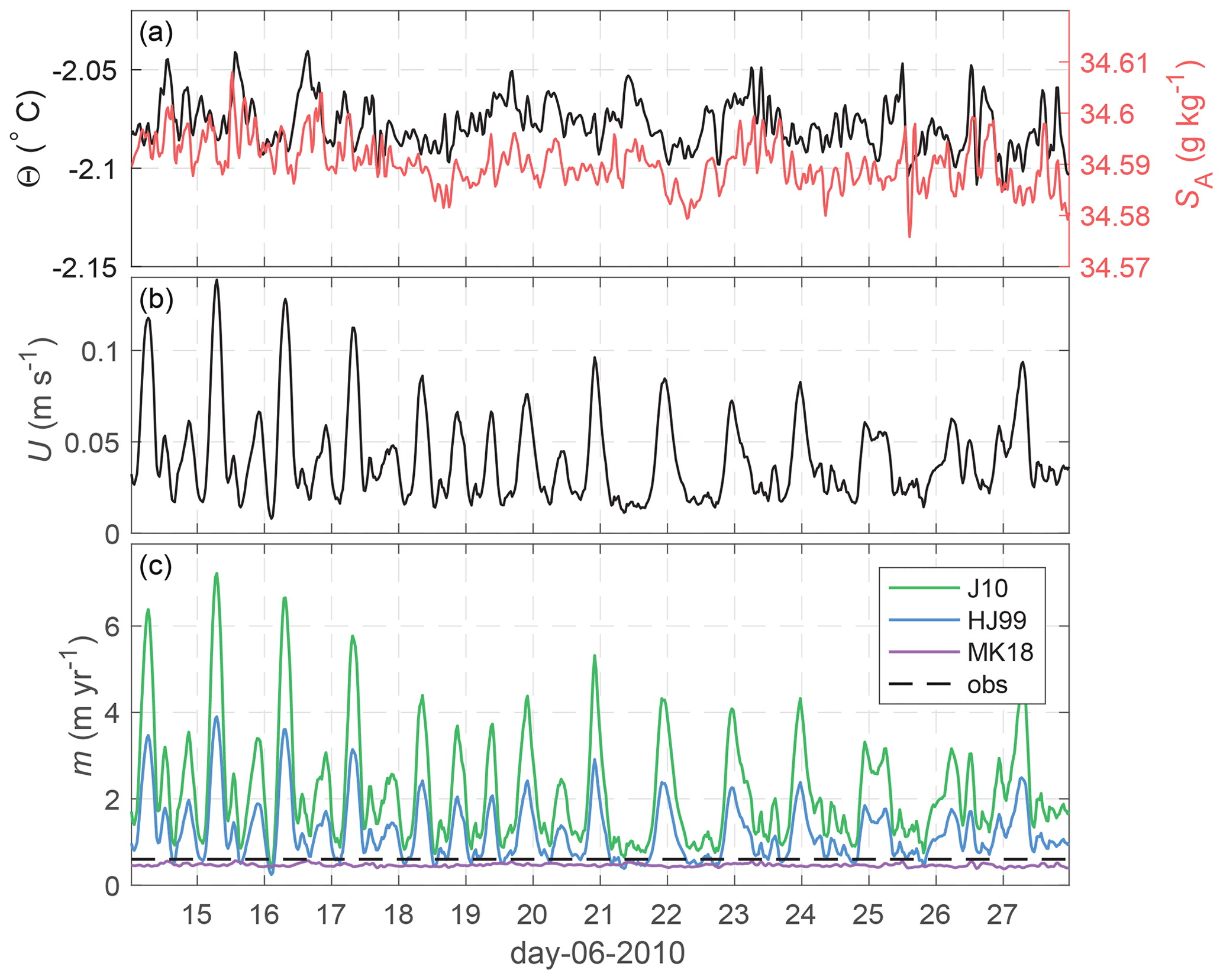
Figure 9(a) Θ and SA from the upper MicroCAT 4 m below the ice, (b) current speed depth-averaged over 7–19 m below the ice base, and (c) parameterised melt rates for the three parameterisations compared in this study. While the J10 and HJ99 melt rates are strongly modulated by the tidal currents at AM06, MK18 varies only with temperature.
The J10, HJ99, and MK18 parameterisations are applied to a short slice of observational data to show how they respond to ocean forcing (Fig. 9). The shear-dependent parameterisations exhibit large variability in melting on short timescales due to the tidal flow at AM06, which varies between 1 and 14 cm s−1 over a 2-week period (Fig. 9). The convective parameterisation does not vary much on these timescales, as variability is driven solely by small amplitude temperature fluctuations. Both the J10 and HJ99 parameterisations predict much higher melt rates than are observed, while the MK18 convective parameterisation prediction is close to observations over this period.
The parameterisations are evaluated quantitatively by comparing the time-mean of the predicted melt rate and the observed melt rate (Table 3). The parameterisation that best fits the observations is the convective parameterisation (MK18) based on the local slope angle, which is biased 20 % low over period February–November. However, despite predicting the annual average melt rate quite well, the seasonal variation in mMK18 is much smaller than in the observed melt rate.
The shear-dependent parameterisations (HJ99 and J10) are only evaluated over the period April–November due to poor velocity data return near the ice in the early months of 2010. J10 melt rates are 400 % larger than the observed melt rates, while HJ99 melt rates are roughly 200 % the observations. In all cases, the fit worsens by ∼ 6 % if the heat flux into the ice is neglected. Again, neither parameterisation captures the seasonal variation of the melting (Table 3), indicating an issue with the functional form of the parameterisation. This is further highlighted for the J10 parameterisation by the best-fit Stanton number , which is obtained by solving Eqs. (A1)–(A3) given the observed melt rate and assuming = 35. The best-fit Stanton number also varies considerably between the different averaging periods. For example, we find = 0.00017 for the July–September period, while we find = 0.00031 for April–June. The fact that one value cannot be used year-round suggests that the functional form of J10 is not appropriate for all AM06 conditions.
The best fit for the period April–November is 0.00027, much lower than the recommended value from the Filchner–Ronne site of 0.0011 from Jenkins et al. (2010b). In this formulation, it is expected that ΓT is constant, whereas Cd is determined by the frictional properties of the ice base and is therefore site dependent. Based on their Filchner–Ronne data Jenkins et al. (2010b) suggest ΓT = 0.011. In order to reconcile this value with our observed Stanton number we would need an extremely low drag coefficient (Cd = 0.0006) at AM06.
CTD profiles taken at the beginning of the observational period (Fig. 2) measure a temperature gradient of = 0.0017 over the upper 10 m of the water column. Accordingly, if the melt rate calculated using J10 for Θ(d=4) is 2 m yr−1, taking Θ(d=1) yields 1.95 m yr−1 while Θ(d=10) results in 2.1 m yr−1.
4.4 Is it appropriate to apply a convective melting parameterisation at AM06?
Despite the relatively good agreement between observed melting and the MK18 convective melting parameterisation, it is not altogether clear that this parameterisation is appropriate for AM06 due to the presence of tidal currents. The MK18 parameterisation does not depend on current speed (tidal or residual) and is not expected to hold in the presence of strong currents. In laboratory experiments, McConnochie and Kerr (2017a) observe a transition from convectively controlled to shear-controlled melting at a velocity of 2–4 cm s−1 for 0.5 ∘C. The typical time-mean flow speed at AM06 (U7–19) is ∼ 4.0 cm s−1, while instantaneous speeds can be in excess of 15 cm s−1, suggesting that AM06 should be well within the shear-controlled melting regime. However, the effects of a small slope angle and ambient stratification are not taken into account in this transition, which was determined for vertical ice.
In their study, Malyarenko et al. (2020) found that the convective melting parameterisation for a vertical ice face from Kerr and McConnochie (2015) captured observed melt rates well at sites on the Ross and Filchner–Ronne ice shelves during times where the Reynolds number for the diffusive sublayer () was low, despite being applied to ice shelves with a shallow mean slope. Based on these sites, they suggest a critical Reδ for the convective-shear transition of ∼ 20. Following the same methodology (see Sect. 6.3 of Malyarenko et al., 2020), we find Reδ∼ 13 for the time-mean conditions over the April–December period (Table 3; row 5), lending support to the idea that convective melting may dominate at AM06.
An important consideration for parameterising melt as a function of ice shelf slope in regional ocean models is the ice shelf basal topography. Here, we apply the MK18 parameterisation to the local slope measured by the ADCP; however, features such as our basal “scarp” (Fig. 7) or the basal terraces observed beneath Pine Island Glacier (Dutrieux et al., 2014) will be subgrid-scale in circumpolar or regional-scale ocean models that have kilometre-scale resolution beneath ice shelves (e.g. Naughten et al., 2018b). Consequently, melting would be underestimated. For example, if we use a basal slope of θ = 0.2∘ rather than 9∘ at the AM06 site, the MK18 parameterisation predicts a melt rate of ∼ 3 cm yr−1. As such, while the convective melt rate parameterisation is a relatively good fit for our observations, significant challenges remain for the implementation of a slope-dependent parameterisation in ocean models where small-scale variations in basal slope are not resolved.
4.5 Comparison with other direct melt rate measurements
Here we extend the comparison between observed and parameterised melt rates to include other published studies of ice shelf melt rate and in situ ocean observations from around Antarctica. Due to limitations in the data available this comparison is only made for the J10 parameterisation. The observed and parameterised melt rates, mean thermal forcing, and current speed at each location are presented in Table 4, where the data are sourced from the relevant publications. More detail on the observational data is provided in the footnote of Table 4.
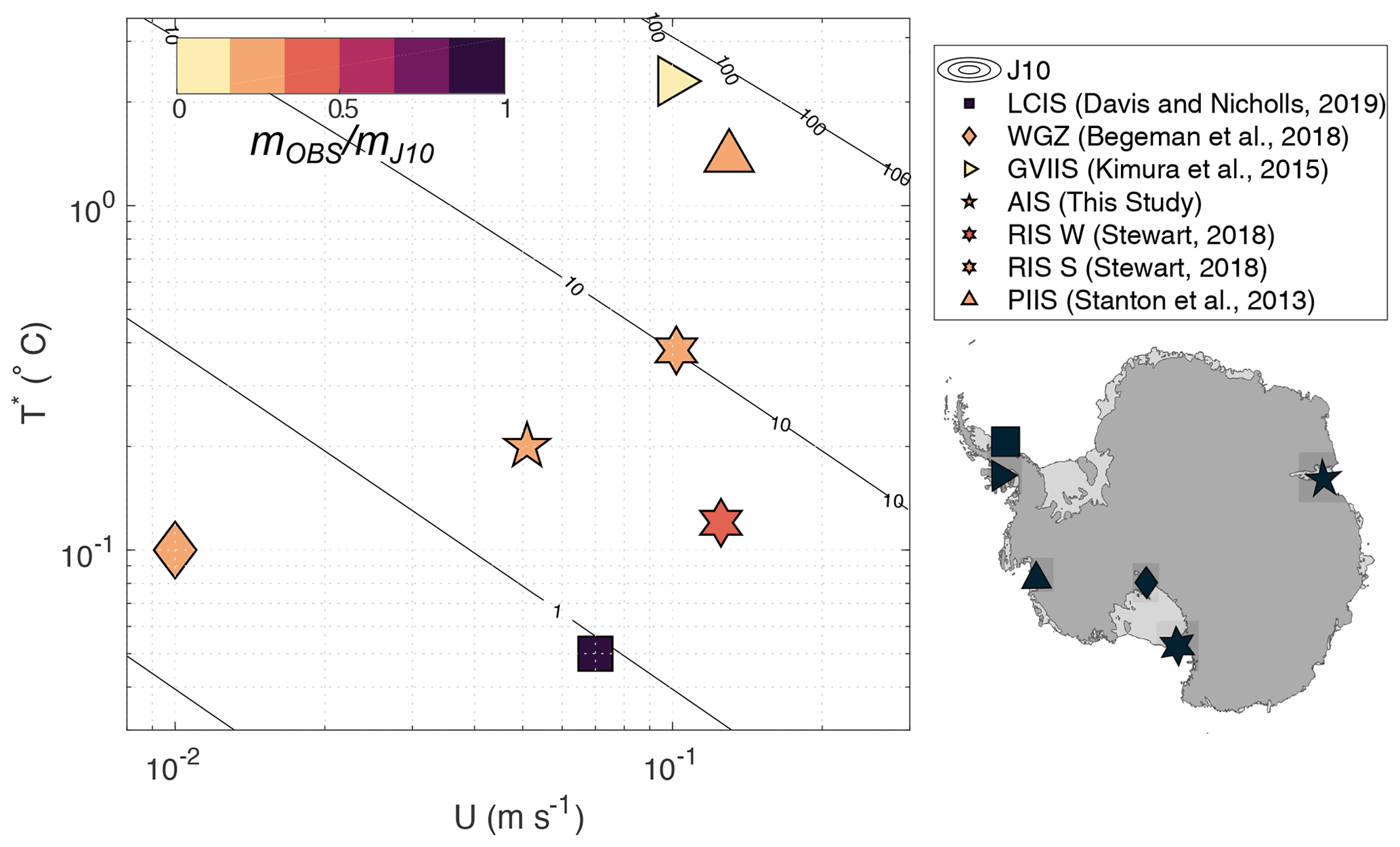
Figure 10Ratio of observed (mOBS) to predicted melt rate for the J10 parameterisation (mJ10) as a function of thermal driving (T∗) and free stream velocity (U) for published ice shelf datasets. Contours show mJ10. Map shows the location of the observations.
The ratio of observed to parameterised melt rates is plotted as a function of the local thermal driving and flow speed in Fig. 10. The J10 parameterisation significantly overpredicts melt rates at many locations, particularly at warm and quiescent conditions. For example, beneath George VI Ice Shelf, where thermal driving is extremely high, predicted melt rates are ∼ 5000 % of the observed values ( = 0.02). The exception to this is beneath the Larsen C Ice Shelf (Davis and Nicholls, 2019). This is unsurprising, since the Larsen C site is characterised by low thermal driving ( 0.05 ∘C) and strong, tidally dominated flow, much like the Filchner–Ronne Ice Shelf site, to which the J10 transfer coefficients were tuned. Note that we cannot tune to make the J10 parameterisation fit all the observations in Fig. 10, indicating that a parameterisation of this functional form is not applicable over the full range of observed conditions (i.e. that the oceanic heat flux is not proportional to as in Eq. A2) and/or that cannot be assumed constant.
There are many reasons why J10, a shear-dependent parameterisation, may not accurately reproduce melt rates, especially under warm and quiescent conditions. For example, another mechanism such as convection (Kerr and McConnochie, 2015; Mondal et al., 2019) or double-diffusive convection may be the dominant process driving melting. Stratification effects, a poorly constrained drag coefficient, or an inappropriate choice of input variables may also result in inaccurate melt rate predictions. In high-resolution models, double-diffusive convection has been shown to drive melting beneath ice shelves under warm, low shear conditions (Middleton et al., 2021), forming a thermohaline staircase beneath the ice (Rosevear et al., 2021). Observations of a thermohaline staircase beneath George VI Ice Shelf (Kimura et al., 2015), which is subject to extremely high thermal driving, suggest that double-diffusive convection may drive melting there. Similarly, double-diffusive convection may play a role in melting at the quiescent grounding line of the Ross Ice Shelf (Begeman et al., 2018). Both these sites are characterised by strong thermal forcing relative to the current speed.
For shear-dominated melting, surface buoyancy flux due to meltwater can inhibit vertical fluxes, decreasing the efficiency of heat and salt transfer (Vreugdenhil and Taylor, 2019). Thus, stratification effects may be responsible for the misfit between the parameterised and observed melt rates at AM06 and other sites. For example, a decrease in the efficiency of heat transport could explain the poor performance of the J10 parameterisation for the Amery (this study) and Ross (Stewart, 2018) ice shelf sites which have similar current speeds to, but much higher thermal driving than, the Larsen C and Filchner–Ronne sites.
Another possible source of discrepancy between observed and parameterised melt rates is the drag coefficient. At AM06, a lack of information about the frictional properties of the ice base forces an arbitrary choice of Cd in order to apply the shear-dependent parameterisations to the oceanographic data. This issue is not just specific to our study – in general, Cd is extremely poorly constrained beneath ice shelves (e.g. Gwyther et al., 2015). Furthermore, Cd is often used as a tuning parameter when attempting to reconcile observed and parameterised melt rates (e.g. Jenkins et al., 2010b; Nicholls, 2018). In ice–ocean models, drag coefficients in the range 0.0015–0.003 are typically used (e.g. MacAyeal, 1984; Gwyther et al., 2015; Naughten et al., 2018b). Recent turbulence measurements beneath the Larsen C Ice Shelf were used to infer a drag coefficient of Cd = 0.0022 at a melting site with a cold, unstratified, tidally forced ISOBL (Davis and Nicholls, 2019). Beneath melting sea ice, values in the range 0.0025–0.01 have been measured (McPhee, 1992), while values in excess of 0.01 have been observed beneath sea ice in the presence of rough platelet ice (Robinson et al., 2017). The drag coefficient Cd = 0.0097 recommended by Jenkins et al. (2010b) is within this range of estimates.
Poor agreement between the parameterised and observed melt rates may be a result of the depth at which the temperature, salinity and velocity are measured. At AM06 we observe that the boundary layer beneath the ice is stratified in both temperature and salinity, contrary to the paradigm of a well-mixed ISOBL on which the three-equation parameterisation is based. Other borehole measurements such as those in the McMurdo (Robinson et al., 2010) and George VI (Kimura et al., 2015) ice shelves also show stratification in temperature and salinity below the ice. Near the calving front of the Ross Ice Shelf, the absence of a well-mixed layer beneath the ice was found to reduce the fit between the three-equation parameterisation and the observed melt rates (Stewart, 2018), and result in a sub-linear dependence of melt rate on temperature. The importance of measuring the current speed at an appropriate depth has also been demonstrated. Beneath the Larsen C Ice Shelf, Davis and Nicholls (2019) found that at low flow speeds – when their fixed-depth velocity measurements were taken outside of the log layer – the drag relationship (Eq. A4) did not estimate the friction velocity accurately, introducing large errors in the predicted melt rate. In the presence of steep basal topography, the problem of correctly identifying the depth at which Θ, SA and U should be sampled becomes even more challenging. For example, the basal scarp observed at AM06 may result in acceleration, stagnation, or separation of the flow. Consequently U7–19, which we use to predict melting, may not be representative of the flow speed next to the ice. Finally, we highlight that these issues are not limited to observational studies. The numerical models for which these parameterisations were developed are also sensitive to the choice of sampling depth, as well as the way in which the meltwater flux is distributed (Gwyther et al., 2020). Sampling and distributing meltwater at the upper grid cell introduces a dependence of the melt rate on the model grid resolution.
(Jenkins et al., 2010b)(Davis and Nicholls, 2019)(Kimura et al., 2015)(Stewart, 2018)(Stewart, 2018)(Stanton et al., 2013)(Begeman et al., 2018)Table 4Comparison between observed and predicted melt rates for a series of Antarctic ice shelves for which both melt rates and in situ oceanographic data are available. Observed variables presented are the time-mean current speed (), time-mean friction velocity (), thermal driving (), and melt rate (mOBS). Melt rate predictions made from J10 are also presented for each site. Where they are in bold, we have used the estimate from the original study. In the final column we note sites with a strong tidal component to the flow.
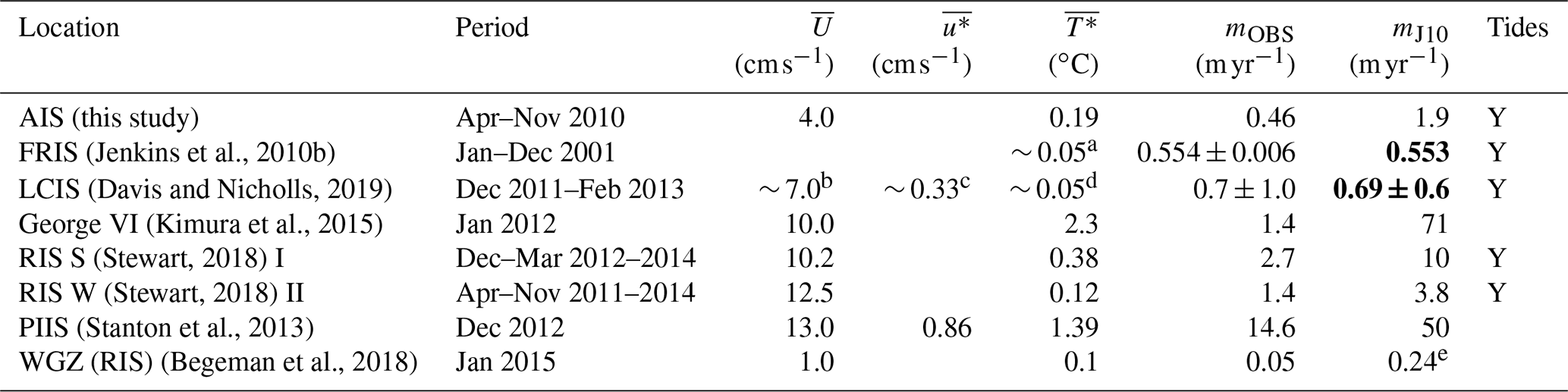
a Value obtained from visual inspection of Fig. 4 of Jenkins et al. (2010b). Value should be considered approximate only. b Calculated from Fig. 3 of Davis and Nicholls (2019) (upper instrument). Value should be considered approximate only. c Calculated from and observed drag coefficient Cd = 0.0022. d Mixed-layer temperature TML = −2.06–2.04 ∘C (from temperature profile in Fig. 2b or from text of Davis and Nicholls, 2019). Using SML = 34.54 psu and pi = 304 dbar, Tf = − 7.53 × 10⁻⁴ pi yields T∗ = 0.04–0.06 ∘C. Value should be considered approximate only. e This value differs from the reported value of 0.15 in Begeman et al. (2018). The discrepancy may be due to the inclusion of the conductive ice shelf heat flux by Begeman et al. (2018) or the use of a different drag coefficient other than the Cd = 0.0097 suggested in Jenkins et al. (2010b).
In this paper we examined the relationship between basal melting and ocean conditions beneath the AIS using mooring data from a borehole drilled in 2010. The mooring location is characterised by the year-round presence of ISW derived from HSSW. The ISW is consistently warmer than the in situ freezing temperature, indicating that it originates from a shallower depth within the cavity. The mean flow is oriented into the cavity at 220∘ N and exhibits little vertical shear over the upper 100 m of the water column. We hypothesise a mainly barotropic flow advecting HSSW from the calving front, which is modified by the addition of meltwater to become ISW as it travels beneath the ice shelf and past AM06. This is consistent with picture of cavity circulation that varies longitudinally, with HSSW inflow on the eastern flank of the cavity and outflow of ISW in the west. Basal melting at the site is a modest 0.51 ± 0.18 m yr−1 and varies seasonally with temperature and salinity. The warmest conditions and highest melt rates are observed in the austral autumn, and the coolest and lowest melt conditions are observed in the austral spring. The springtime minimum in melt is coincident with the most highly meltwater-modified conditions at AM06, as well as the weakest residual flow. Tides dominate current variability, driving current speeds of ∼ 10 cm s−1, while the superposition of the tidal and mean flow can result in flow speeds in excess of ∼ 15.0 cm s−1. A large scarp (∼ 20 m in height) was discovered in the underside of the ice shelf using the upward-looking ADCP, adding to our growing understanding of the spatial complexity of ice shelf basal topography. In addition, we have demonstrated the utility of an upward-looking ADCP for field studies of ice shelf–ocean interactions. We were able to measure basal melt rates and ocean velocities and produce a map of the underside of the ice base with a single instrument, demonstrating the advantage over a single-beam acoustic instrument, such as an upward-looking sonar (Stewart et al., 2019).
In situ oceanographic and melt rate observations were used to evaluate common ice–ocean parameterisations. Despite the presence of tidal currents, we found that the convective, slope-dependent ice shelf parameterisation of McConnochie and Kerr (2018) was the best performing of the three parameterisations tested at AM06, underestimating observed melt rates by ∼ 20 %. The velocity-dependent parameterisations of Jenkins et al. (2010b) and Holland and Jenkins (1999) overestimated melting by 400 % and 200 %, respectively. None of the parameterisations reproduced the seasonality variation in melting. Extension of our analysis to other published studies of in situ oceanographic data demonstrated that the misfit between the Jenkins et al. (2010b) parameterisation and observations is widespread in temperature–velocity space: the parameterisation only performs well under the coldest, most energetic conditions. Previous studies have shown that this parameterisation performs poorly for warm and/or quiescent conditions. However, here we have shown that even cold-cavity ice shelves such as the Ross and Amery Ice Shelves, which have strong currents and only moderate (0.1–0.5 ∘C) thermal driving, are not well represented by this parameterisation. The systematic bias of the J10 melt rates at warmer and/or quiescent conditions indicates that the functional form of this parameterisation is not applicable over the full range of observed conditions and that cannot be assumed constant. Our results suggest that understanding the effects of buoyancy on the ISOBL is a critical area for future studies aiming to improve parameterisations of basal melting in ocean climate models.
A1 Shear-controlled melting
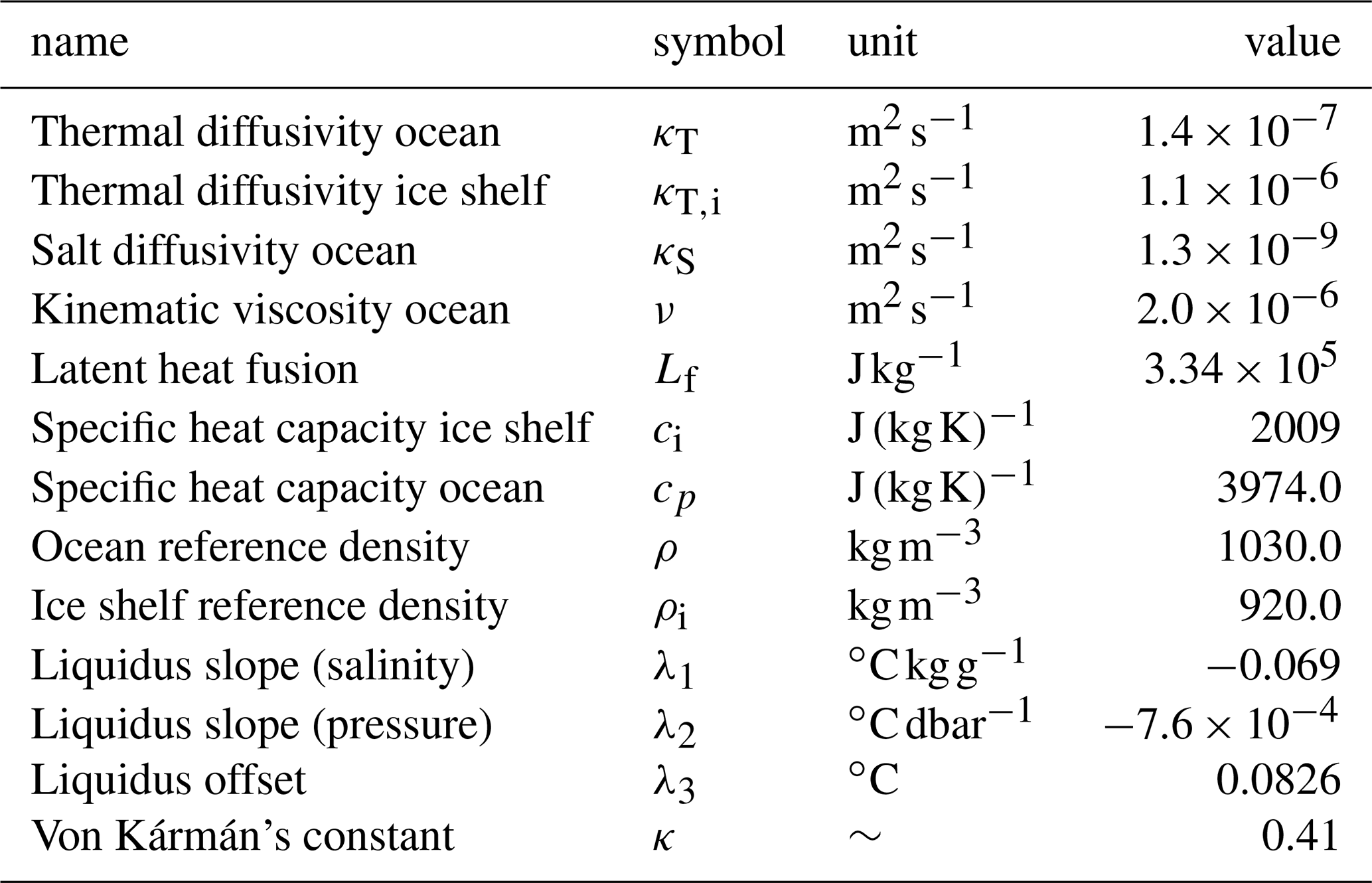
The Holland and Jenkins (1999) and Jenkins et al. (2010a) parameterisations take the same general form. The interface temperature Tb is assumed to be at freezing temperature at interface salinity and pressure , where interface temperature and salinity are related by the linearised liquidus relationship:
The physical parameters λ1, λ2, and λ3 are described in Table A1.
Table A1Physical parameters used in melt parameterisation calculations.
At the ice–ocean interface, the divergence of heat is balanced by a latent heat flux due to melting, with an equivalent balance for salt. The ice shelf melt rate (m) appears in the latent heat (Qlatent=Lfmρi) and brine (Qbrine=Sbmρi) fluxes, respectively, where Lf is the latent heat of freezing and ρi is the ice density. The heat balance expression is given by
where the first term on the right-hand side is the diffusive heat flux into the ice shelf, is the ice shelf vertical temperature gradient evaluated at the ice–ocean interface, and ci and κT,i are the heat capacity and thermal diffusivity of the ice, respectively. The second term on the right-hand side is the oceanic heat flux, here parameterised in terms of the bulk temperature difference across the boundary layer (Tb−TML, where TML denotes the mixed-layer temperature), the friction velocity u∗ and a transfer coefficient ΓT. Parameters ρ and cp are the density and heat capacity of the ocean mixed layer, respectively. An equivalent expression is given for the balance of salt:
where ΓS is the salt transfer coefficient. In this expression the ice salinity and the diffusive salt flux within the ice are assumed to be zero. The friction velocity (u∗) is defined as the square root of the kinematic stress at the ice–ocean interface. However, in ocean models u∗ is typically estimated as a function of the free-stream current speed (U) through a simple parameterisation:
where drag coefficient Cd is often taken to be 0.0025 (Gwyther et al., 2015).
A1.1 Holland and Jenkins (1999): flow-dependent transfer coefficients
Holland and Jenkins (1999) use Eqs. (A1)–(A3) with transfer coefficients (ΓT, ΓS) from the sea ice literature (McPhee et al., 1987):
where Pr (Sc) is the Prandtl (Schmidt) number, κ=0.4 is von Kármán's constant, f is the Coriolis parameter, ξ=0.052 is a dimensionless constant, and is the thickness of the viscous sublayer. The stability parameter (η) describes the influence of an interfacial buoyancy flux, which reduces the ISOBL depth. The buoyancy flux is itself determined by the melt rate. For η=1, the parameterisation becomes analogous to that used by Jenkins (1991). Equations (A2) and (A3) are functions of u∗.
A1.2 Jenkins et al. (2010): constant transfer coefficients
Jenkins et al. (2010b) used ice shelf melting, upper-ocean temperature, and current meter measurements to observationally constrain these transfer coefficients. As u∗ was not directly measured, they inverted for the products and , which they term thermal and saline Stanton numbers, using Eq. (A4) and assuming constant Cd. The best fit to the data was found for = 0.0011 and = 3.1 × 10⁻⁵, assuming the ratio = 35. Drawing on results from the sea ice literature (McPhee, 2008), they recommend the values Cd = 0.0097, ΓS = 3.1 × 10⁻⁴, and ΓT = 0.011.
A2 McConnochie and Kerr (2018): convection-controlled melting
In the convective melting parameterisation of Kerr and McConnochie (2015), extended to sloping ice in McConnochie and Kerr (2018), the interface temperature is given by
where κT and κS are the molecular diffusivities of heat and salt and the subscript ∞ denotes the ambient ocean values. The melt rate is then given by
where γ is a constant equal to 0.09 (Kerr and McConnochie, 2015) and θ is the angle of the ice–ocean interface to the horizontal. Using the liquidus relationship (Eq. A1), this system of equations can be solved for Tb, Sb and m.
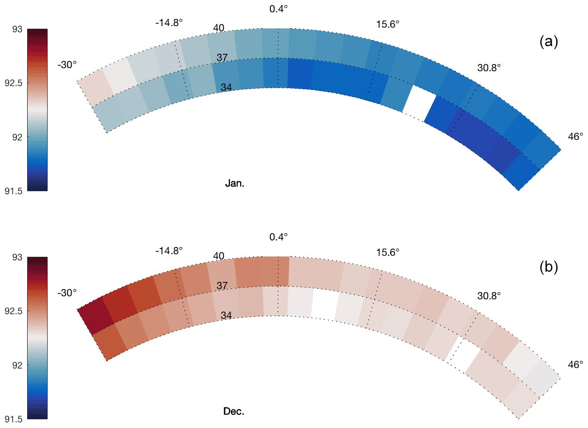
Figure B1Range from the ADCP to the ice base in metres (colour) in January (a) and December (b) in polar coordinates.

Figure B2(a) Hovmöller plot of current speed in depth and time over a week-long period, with the 1 d quiver plot indicating the depth-mean current direction. (b) Histogram of the ratio between velocity in the bin at 7 m (U7) and the four-bin-average velocity over 7–19 m depth (U7–19) for the whole dataset.

Figure B3(a) Heat flux into the ice () as a function of melt rate m from a one-dimensional advection–diffusion model for a 607 m thick ice shelf with a −20 ∘C surface and −2.1 ∘C basal temperature. (b) Ratio of to latent heat flux due to melting as function of m. The vertical dashed lines correspond to the annual average melt rate of 0.51 m yr−1.
The data used in this study are available at https://data.aad.gov.au/metadata/records/ASAC_1164_AM06 (Allison and Craven, 2013) and https://doi.org/10.26179/r16w-am36 (Rosenberg et al., 2021).
BGF and MR designed the research. MR performed the analysis. MR, CS, and BGF contributed to interpretation of results and writing.
The contact author has declared that none of the authors has any competing interests.
Publisher's note: Copernicus Publications remains neutral with regard to jurisdictional claims in published maps and institutional affiliations.
We acknowledge logistical support from the Australian Antarctic Division and the many people who contributed to the AMISOR project, Li Yuansheng (Polar Research Institute of China) for supplying the ADCP used in this study, Mark Rosenberg for data quality control, and Rebecca Cowley for technical advice. We also wish to acknowledge Carolyn Begeman and an anonymous reviewer for their constructive comments which greatly improved this paper.
This research was supported under the Australian Research Council's Special Research Initiative for Antarctic Gateway Partnership (project ID SR140300001). Ben Galton-Fenzi received grant funding from the Australian Government as part of the Antarctic Science Collaboration Initiative program (ASCI000002). Craig Stevens is supported by the New Zealand Antarctic Science Platform (ANTA1801).
This paper was edited by Matthew Hecht and reviewed by Carolyn Begeman and one anonymous referee.
Adusumilli, S., Fricker, H. A., Siegfried, M. R., Padman, L., Paolo, F. S., and Ligtenberg, S. R. M.: Variable Basal Melt Rates of Antarctic Peninsula Ice Shelves, 1994–2016, Geophys. Res. Lett., 45, 4086–4095, https://doi.org/10.1002/2017GL076652, 2018. a
Adusumilli, S., Fricker, H. A., Medley, B., Padman, L., and Siegfried, M. R.: Interannual variations in meltwater input to the Southern Ocean from Antarctic ice shelves, Nat. Geosci., 13, 616–620, https://doi.org/10.1038/s41561-020-0616-z, 2020. a, b
Allison, I.: The AMISOR project: ice shelf dynamics and ice-ocean interaction of the Amery Ice Shelf, FRISP Report, 14, 1–9, https://folk.uib.no/ngfso/FRISP/Rep14/allison.pdf (last access: 18 July 2022), 2003. a
Allison, I. and Craven, M.: Amery Ice Shelf – hot water drill borehole, AM06 Seabird MicroCAT CTD moorings at three depths in ocean cavity beneath the shelf, Ver. 1, Australian Antarctic Data Centre [data set], https://doi.org/10.4225/15/525F34127651E, 2013. a
Arzeno, I. B., Beardsley, R. C., Limeburner, R., Owens, B., Padman, L., Springer, S. R., Stewart, C. L., and Williams, M. J.: Ocean variability contributing to basal melt rate near the ice front of Ross Ice Shelf, Antarctica, J. Geophys. Res.-Oceans, 119, 4214–4233, https://doi.org/10.1002/2014JC009792, 2014. a
Bamber, J. L., Westaway, R. M., Marzeion, B., and Wouters, B.: The land ice contribution to sea level during the satellite era, Environ. Res. Lett., 13, 063008, https://doi.org/10.1088/1748-9326/aac2f0, 2018. a
Begeman, C. B., Tulaczyk, S. M., Marsh, O. J., Mikucki, J. A., Stanton, T. P., Hodson, T. O., Siegfried, M. R., Powell, R. D., Christianson, K., and King, M. A.: Ocean Stratification and Low Melt Rates at the Ross Ice Shelf Grounding Zone, J. Geophys. Res.-Oceans, 123, 7438–7452, https://doi.org/10.1029/2018JC013987, 2018. a, b, c, d
Cook, A. J., Holland, P. R., Meredith, M. P., Murray, T., Luckman, A., and Vaughan, D. G.: Ocean forcing of glacier retreat in the western Antarctic Peninsula, Science, 353, 283–286, https://doi.org/10.1126/science.aae0017, 2016. a, b
Craven, M., Allison, I., Brand, R., Elcheikh, A., Hunter, J., Hemer, M., and Donoghue, S.: Initial borehole results from the Amery Ice Shelf hot-water drilling project, Ann. Glaciol., 39, 531–539, https://doi.org/10.3189/172756404781814311, publisher: Cambridge University Press, 2004. a
Craven, M., Warner, R. C., Vogel, S. W., and Allison, I.: Platelet ice attachment to instrument strings beneath the Amery Ice Shelf , East Antarctica, J. Glaciol., 60, 383–393, https://doi.org/10.3189/2014JoG13J082, 2014. a
Davis, P. E. and Nicholls, K. W.: Turbulence Observations beneath Larsen C Ice Shelf, Antarctica, J. Geophys. Res.-Oceans, 124, 5529–5550, https://doi.org/10.1029/2019JC015164, 2019. a, b, c, d, e, f
Depoorter, M. A., Bamber, J. L., Griggs, J. A., Lenaerts, J. T. M., Ligtenberg, S. R. M., Broeke, M. R. V. D., and Moholdt, G.: Calving fluxes and basal melt rates of Antarctic ice shelves, Nature, 502, 89–92, https://doi.org/10.1038/nature12567, 2013. a, b
Dinniman, M., Asay-Davis, X., Galton-Fenzi, B., Holland, P., Jenkins, A., and Timmermann, R.: Modeling ice shelf/ocean interaction in Antarctica: A review, Oceanography, 29, 144–153, https://doi.org/10.5670/oceanog.2016.106, 2016. a
Dupont, T. K. and Alley, R. B.: Assessment of the importance of ice-shelf buttressing to ice-sheet flow, Geophys. Res. Lett., 32, L04503, https://doi.org/10.1029/2004GL022024, 2005. a
Dutrieux, P., Stewart, C., Jenkins, A., Nicholls, K. W., Corr, H. F., Rignot, E., and Steffen, K.: Basal terraces on melting ice shelves, Geophys. Res. Lett., 41, 5506–5513, https://doi.org/10.1002/2014GL060618, 2014. a, b, c
Fretwell, P., Pritchard, H. D., Vaughan, D. G., Bamber, J. L., Barrand, N. E., Bell, R., Bianchi, C., Bingham, R. G., Blankenship, D. D., Casassa, G., Catania, G., Callens, D., Conway, H., Cook, A. J., Corr, H. F. J., Damaske, D., Damm, V., Ferraccioli, F., Forsberg, R., Fujita, S., Gim, Y., Gogineni, P., Griggs, J. A., Hindmarsh, R. C. A., Holmlund, P., Holt, J. W., Jacobel, R. W., Jenkins, A., Jokat, W., Jordan, T., King, E. C., Kohler, J., Krabill, W., Riger-Kusk, M., Langley, K. A., Leitchenkov, G., Leuschen, C., Luyendyk, B. P., Matsuoka, K., Mouginot, J., Nitsche, F. O., Nogi, Y., Nost, O. A., Popov, S. V., Rignot, E., Rippin, D. M., Rivera, A., Roberts, J., Ross, N., Siegert, M. J., Smith, A. M., Steinhage, D., Studinger, M., Sun, B., Tinto, B. K., Welch, B. C., Wilson, D., Young, D. A., Xiangbin, C., and Zirizzotti, A.: Bedmap2: improved ice bed, surface and thickness datasets for Antarctica, The Cryosphere, 7, 375–393, https://doi.org/10.5194/tc-7-375-2013, 2013. a
Fricker, H. A., Popov, S., Allison, I., and Young, N.: Distribution of marine ice beneath the Amery Ice Shelf, Geophys. Res. Lett., 28, 2241–2244, https://doi.org/10.1029/2000GL012461, 2001. a, b
Fürst, J. J., Durand, G., Gillet-Chaulet, F., Tavard, L., Rankl, M., Braun, M., and Gagliardini, O.: The safety band of Antarctic ice shelves, Nat. Clim. Change, 6, 479–482, https://doi.org/10.1038/nclimate2912, 2016. a
Gade, H. G.: Melting of ice in sea water: A primitive model with application to the Antarctic ice shelf and icebergs, J. Phys. Oceanogr., 9, 189–198, https://doi.org/10.1175/1520-0485(1979)009<0189:MOIISW>2.0.CO;2, 1979. a, b
Galton-Fenzi, B. K.: Modelling ice-shelf/ocean interaction, PhD thesis, University of Tasmania, https://eprints.utas.edu.au/19882/ (last access: 18 July 2022), 2009. a
Galton-Fenzi, B. K., Hunter, J. R., Coleman, R., Marsland, S. J., and Warner, R. C.: Modeling the basal melting and marine ice accretion of the Amery Ice Shelf, J. Geophys. Res.-Oceans, 117, 1–19, https://doi.org/10.1029/2012JC008214, 2012. a, b, c, d, e, f, g, h, i, j
Gayen, B., Griffiths, R. W., and Kerr, R. C.: Simulation of convection at a vertical ice face dissolving into saline water, J. Fluid Mech., 798, 284–298, https://doi.org/10.1017/jfm.2016.315, 2016. a, b, c
Greene, C.: Ice flowlines, MATLAB Central File Exchange, https://www.mathworks.com/matlabcentral/fileexchange/53152-ice-flowlines, (last access: 4 April 2022), 2022. a
Greene, C. A., Gwyther, D. E., and Blankenship, D. D.: Antarctic mapping tools for MATLAB, Comput. Geosci., 104, 151–157, https://doi.org/10.1016/j.cageo.2016.08.003, 2017. a
Gwyther, D. E., Galton-Fenzi, B. K., Dinniman, M. S., Roberts, J. L., and Hunter, J. R.: The effect of basal friction on melting and freezing in ice shelf-ocean models, Ocean Model., 95, 38–52, https://doi.org/10.1016/j.ocemod.2015.09.004, 2015. a, b, c
Gwyther, D. E., Cougnon, E. A., Galton-Fenzi, B. K., Roberts, J. L., Hunter, J. R., and Dinniman, M. S.: Modelling the response of ice shelf basal melting to different ocean cavity environmental regimes, Ann. Glaciol., 57, 131–141, https://doi.org/10.1017/aog.2016.31, 2016. a, b
Gwyther, D. E., Kusahara, K., Asay-Davis, X. S., Dinniman, M. S., and Galton-Fenzi, B. K.: Vertical processes and resolution impact ice shelf basal melting: A multi-model study, Ocean Model., 147, 101569, https://doi.org/10.1016/j.ocemod.2020.101569, 2020. a
Hattermann, T., Nøst, O. A., Lilly, J. M., and Smedsrud, L. H.: Two years of oceanic observations below the Fimbul Ice Shelf, Antarctica, Geophys. Res. Lett., 39, L12605, https://doi.org/10.1029/2012GL051012, 2012. a
Hellmer, H. H. and Olbers, D.: A two-dimensional model for the thermohaline circulation under an ice shelf, Antarct. Sci., 1, 325–336, https://doi.org/10.1017/S0954102089000490, 1989. a
Hemer, M., Hunter, J., and Coleman, R.: Barotropic tides beneath the Amery Ice Shelf, J. Geophys. Res.-Oceans, 111, C11008, https://doi.org/10.1029/2006JC003622, 2006. a
Herraiz-Borreguero, L., Allison, I., Craven, M., Nicholls, K. W., and Rosenberg, M. A.: Ice shelf/ocean interactions under the Amery Ice Shelf: Seasonal variability and its effect on marine ice formation, J. Geophys. Res.-Oceans, 118, 7117–7131, https://doi.org/10.1002/2013JC009158, 2013. a, b, c
Herraiz-Borreguero, L., Coleman, R., Allison, I., Rintoul, S. R., Craven, M., and Williams, G. D.: Circulation of modified Circumpolar Deep Water and basal melt beneath the Amery Ice Shelf, East Antarctica, J. Geophys. Res.-Oceans, 120, 3098–3112, https://doi.org/10.1002/2015JC010697, 2015. a, b, c, d, e, f
Herraiz-Borreguero, L., Church, J. A., Allison, I., Peña-Molino, B., Coleman, R., Tomczak, M., and Craven, M.: Basal melt, seasonal water mass transformation, ocean current variability, and deep convection processes along the Amery Ice Shelf calving front, East Antarctica, J. Geophys. Res.-Oceans, 121, 4946–4965, https://doi.org/10.1002/2016JC011858, 2016. a, b, c, d
Holland, D. M. and Jenkins, A.: Modeling Thermodynamic Ice–Ocean Interactions at the Base of an Ice Shelf, J. Phys. Oceanogr., 29, 1787–1800, https://doi.org/10.1175/1520-0485(1999)029<1787:MTIOIA>2.0.CO;2, 1999. a, b, c, d, e
Huppert, H. E. and Turner, J. S.: On melting icebergs, Nature, 271, 46–48, https://doi.org/10.1038/271046a0, 1978. a
Jackson, P. R. and Rehmann, C. R.: Experiments on differential scalar mixing in turbulence in a sheared, stratified flow, J. Phys. Oceanogr., 44, 2661–2680, https://doi.org/10.1175/JPO-D-14-0027.1, 2014. a
Jacobs, S. S., Jenkins, A., Giulivi, C. F., and Dutrieux, P.: Stronger ocean circulation and increased melting under Pine Island Glacier ice shelf, Nat. Geosci., 4, 519–523, https://doi.org/10.1038/ngeo1188, 2011. a
Jenkins, A.: A one-dimensional model of ice shelf-ocean interaction, J. Geophys. Res.-Oceans, 96, 20671–20677, https://doi.org/10.1029/91JC01842, 1991. a, b
Jenkins, A., Dutrieux, P., Jacobs, S. S., McPhail, S. D., Perrett, J. R., Webb, A. T., and White, D.: Observations beneath Pine Island Glacier in West Antarctica and implications for its retreat, Nat. Geosci., 3, 468–472, 2010a. a, b
Jenkins, A., Nicholls, K. W., and Corr, H. F.: Observation and parameterization of ablation at the base of Ronne Ice Shelf, Antarctica, J. Phys. Oceanogr., 40, 2298–2312, https://doi.org/10.1175/2010JPO4317.1, 2010b. a, b, c, d, e, f, g, h, i, j, k
Jenkins, A., Shoosmith, D., Dutrieux, P., Jacobs, S., Kim, T. W., Lee, S. H., Ha, H. K., and Stammerjohn, S.: West Antarctic Ice Sheet retreat in the Amundsen Sea driven by decadal oceanic variability, Nat. Geosci., 11, 733–738, https://doi.org/10.1038/s41561-018-0207-4, 2018. a
Keitzl, T., Mellado, J. P., and Notz, D.: Reconciling estimates of the ratio of heat and salt fluxes at the ice-ocean interface, J. Geophys. Res.-Oceans, 121, 1063–1084, https://doi.org/10.1002/2015JC010796, 2016. a, b
Kelley, D., Fernando, H., Gargett, A., Tanny, J., and Özsoy, E.: The diffusive regime of double-diffusive convection, Prog. Oceanogr., 56, 461–481, https://doi.org/10.1016/S0079-6611(03)00026-0, 2003. a
Kerr, R. C. and McConnochie, C. D.: Dissolution of a vertical solid surface by turbulent compositional convection, J. Fluid Mech., 765, 211–228, https://doi.org/10.1017/jfm.2014.722, 2015. a, b, c, d, e, f
Khazendar, A., Schodlok, M. P., Fenty, I., Ligtenberg, S. R. M., Rignot, E., and van den Broeke, M. R.: Observed thinning of Totten Glacier is linked to coastal polynya variability, Nat. Commun., 4, 1–9, https://doi.org/10.1038/ncomms3857, 2013. a
Kimura, S., Nicholls, K. W., and Venables, E.: Estimation of Ice Shelf Melt Rate in the Presence of a Thermohaline Staircase, J. Phys. Oceanogr., 45, 133–148, https://doi.org/10.1175/JPO-D-14-0106.1, 2015. a, b, c, d, e
MacAyeal, D. R.: Thermohaline circulation below the Ross Ice Shelf: A consequence of tidally induced vertical mixing and basal melting, J. Geophys. Res.-Oceans, 89, 597–606, https://doi.org/10.1029/JC089iC01p00597, 1984. a
Malyarenko, A., Wells, A. J., Langhorne, P. J., Robinson, N. J., Williams, M. J., and Nicholls, K. W.: A synthesis of thermodynamic ablation at ice-ocean interfaces from theory, observations and models, Ocean Model., 154, 101692, https://doi.org/10.1016/j.ocemod.2020.101692, 2020. a, b, c, d
McConnochie, C. D. and Kerr, R. C.: The effect of a salinity gradient on the dissolution of a vertical ice face, J. Fluid Mech., 791, 589–607, https://doi.org/10.1017/jfm.2016.62, 2016. a, b
McConnochie, C. D. and Kerr, R. D.: Testing a common ice-ocean parameterization with laboratory experiments, J. Geophys. Res.-Oceans, 122, 5905–5915, https://doi.org/10.1002/2017JC012918, 2017a. a
McConnochie, C. D. and Kerr, R. C.: Enhanced ablation of a vertical ice wall due to an external freshwater plume, J. Fluid Mech., 810, 429–447, https://doi.org/10.1017/jfm.2016.761, 2017b. a, b
McConnochie, C. D. and Kerr, R. C.: Dissolution of a sloping solid surface by turbulent compositional convection, J. Fluid Mech., 846, 563–577, https://doi.org/10.1017/jfm.2018.282, 2018. a, b, c
McDougall, T. J. and Barker, P. M.: Getting started with TEOS-10 and the Gibbs Seawater (GSW) Oceanographic Toolbox, Scor/Iapso Wg127, p. 28, http://www.teos-10.org/ (last access: 18 July 2022), 2011. a
McDougall, T. J., Barker, P. M., Feistel, R., and Galton-Fenzi, B. K.: Melting of Ice and Sea Ice into Seawater and Frazil Ice Formation, J. Phys. Oceanogr., 44, 1751–1775, https://doi.org/10.1175/JPO-D-13-0253.1, 2014. a, b, c, d
McPhee, M.: Air–ice–ocean interaction: Turbulent ocean boundary layer exchange processes, Springer Science & Business Media, 2008. a, b
McPhee, M. G.: Turbulent heat flux in the upper ocean under sea ice, J. Geophys. Res., 97, 5365, https://doi.org/10.1029/92JC00239, 1992. a
McPhee, M. G., Maykut, G. A., and Morison, J. H.: Dynamics and thermodynamics of the ice/upper ocean system in the marginal ice zone of the Greenland Sea, J. Geophys. Res., 92, 7017, https://doi.org/10.1029/JC092iC07p07017, 1987. a, b, c, d
Meredith, M., Sommerkorn, M., Cassotta, S., Derksen, C., Ekaykin, A., Hollowed, A., Kofinas, G., Mackintosh, A., Melbourne-Thomas, J., Muelbert, M. M. C., Ottersen, G., Pritchard, H., and Schuur, E. A. G.: Polar Regions, in: IPCC Special Report on the Ocean and Cryosphere in a Changing Climate, edited by: Pörtner, H.-O., Roberts, D. C., Masson-Delmotte, V., Zhai, P., Tignor, M., Poloczanska, E., Mintenbeck, K., Alegrí, A., Nicolai, M., Okem, A., Petzold, J., Rama, B., Weyer, N. M., Cambridge University Press, Cambridge, UK and New York, NY, USA, 203–320, https://doi.org/10.1017/9781009157964.005, 2019. a, b
Middleton, L., Vreugdenhil, C. A., Holland, P. R., and Taylor, J. R.: Numerical simulations of melt-driven double-diffusive fluxes in a turbulent boundary layer beneath an ice shelf, J. Phys. Oceanogr., 51, 403–418, https://doi.org/10.1175/JPO-D-20-0114.1, 2021. a, b, c
Minchew, B. M., Gudmundsson, G. H., Gardner, A. S., Paolo, F. S., and Fricker, H. A.: Modeling the dynamic response of outlet glaciers to observed ice-shelf thinning in the Bellingshausen Sea Sector, West Antarctica, J. Glaciol., 64, 333–342, https://doi.org/10.1017/jog.2018.24, 2018. a
Mondal, M., Gayen, B., Griffiths, R. W., and Kerr, R. C.: Ablation of sloping ice faces into polar seawater, J. Fluid Mech., 863, 545–571, https://doi.org/10.1017/jfm.2018.970, 2019. a, b, c, d
Naughten, K. A., Meissner, K. J., Galton-Fenzi, B. K., England, M. H., Timmermann, R., and Hellmer, H. H.: Future projections of Antarctic ice shelf melting based on CMIP5 scenarios, J. Climate, 31, 5243–5261, https://doi.org/10.1175/JCLI-D-17-0854.1, 2018a. a
Naughten, K. A., Meissner, K. J., Galton-Fenzi, B. K., England, M. H., Timmermann, R., Hellmer, H. H., Hattermann, T., and Debernard, J. B.: Intercomparison of Antarctic ice-shelf, ocean, and sea-ice interactions simulated by MetROMS-iceshelf and FESOM 1.4, Geosci. Model Dev., 11, 1257–1292, https://doi.org/10.5194/gmd-11-1257-2018, 2018b. a, b, c
Nicholls, K. W.: The study of ice shelf-ocean interaction–techniques and recent results, Advances in Polar Science, 5, 222–230, https://doi.org/10.13679/j.advps.2018.3.00222, 2018. a
Nicholls, K. W., Makinson, K., and Østerhus, S.: Circulation and water masses beneath the northern Ronne Ice Shelf, Antarctica, J. Geophys. Res.-Oceans, 109, C12017, https://doi.org/10.1029/2004JC002302, 2004. a
Nicholls, K. W., Abrahamsen, E. P., Buck, J. J. H., Dodd, P. A., Goldblatt, C., Griffiths, G., Heywood, K. J., Hughes, N. E., Kaletzky, A., Lane-Serff, G. F., and Others: Measurements beneath an Antarctic ice shelf using an autonomous underwater vehicle, Geophys. Res. Lett., 33, L08612, https://doi.org/10.1029/2006GL025998, 2006. a, b
Padman, L., Fricker, H. A., Coleman, R., Howard, S., and Erofeeva, L.: A new tide model for the Antarctic ice shelves and seas, Ann. Glaciol., 34, 247–254, https://doi.org/10.3189/172756402781817752, 2002. a
Pawlowicz, R., Beardsley, B., and Lentz, S.: Classical tidal harmonic analysis including error estimates in MATLAB using T TIDE, Comput. Geosci., 28, 929–937, https://doi.org/10.1016/S0098-3004(02)00013-4, 2002. a, b
Post, A., Galton-Fenzi, B., Riddle, M., Herraiz-Borreguero, L., O'Brien, P., Hemer, M., McMinn, A., Rasch, D., and Craven, M.: Modern sedimentation, circulation and life beneath the Amery Ice Shelf, East Antarctica, Cont. Shelf Res., 74, 77–87, https://doi.org/10.1016/j.csr.2013.10.010, 2014. a
Reese, R., Gudmundsson, G. H., Levermann, A., and Winkelmann, R.: The far reach of ice-shelf thinning in Antarctica, Nat. Clim. Change, 8, 53–57, https://doi.org/10.1038/s41558-017-0020-x, 2018. a, b
Rignot, E., Jacobs, S., Mouginot, J., and Scheuchl, B.: Ice Shelf Melting Around Antarctica, Science, 341, 266–270, https://doi.org/10.1126/science.1235798, 2013. a, b
Rignot, E., Mouginot, J., and Scheuchl, B.: MEaSUREs InSAR-Based Antarctica Ice Velocity Map, Version 2, NASA National Snow and Ice Data Center Distributed Active Archive Center, https://doi.org/10.5067/D7GK8F5J8M8R, Boulder, Colorado, USA, 2017. a
Robinson, N. J., Williams, M. J. M., Barrett, P. J., and Pyne, A. R.: Observations of flow and ice-ocean interaction beneath the McMurdo Ice Shelf, Antarctica, J. Geophys. Res.-Oceans, 115, C03025, https://doi.org/10.1029/2008JC005255, 2010. a
Robinson, N. J., Stevens, C. L., and McPhee, M. G.: Observations of amplified roughness from crystal accretion in the sub-ice ocean boundary layer, Geophys. Res. Lett., 44, 1814– 1822, https://doi.org/10.1002/2016GL071491, 2017. a
Rosenberg, M., Galton-Fenzi, B. K., and Gamble Rosevear, M.: Amery Ice Shelf – hot water drill borehole AM06, RDI 300 kHz ADCP ocean velocity data 2010–2011, Ver. 1, Australian Antarctic Data Centre [data set], https://doi.org/10.26179/r16w-am36, 2021. a
Rosevear, M. G., Gayen, B., and Galton-Fenzi, B. K.: The role of double-diffusive convection in basal melting of Antarctic ice shelves, P. Natl. Acad. Sci. USA, 118, e2007541118, https://doi.org/10.1073/pnas.2007541118, 2021. a, b, c
Seroussi, H., Nowicki, S., Payne, A. J., Goelzer, H., Lipscomb, W. H., Abe-Ouchi, A., Agosta, C., Albrecht, T., Asay-Davis, X., Barthel, A., Calov, R., Cullather, R., Dumas, C., Galton-Fenzi, B. K., Gladstone, R., Golledge, N. R., Gregory, J. M., Greve, R., Hattermann, T., Hoffman, M. J., Humbert, A., Huybrechts, P., Jourdain, N. C., Kleiner, T., Larour, E., Leguy, G. R., Lowry, D. P., Little, C. M., Morlighem, M., Pattyn, F., Pelle, T., Price, S. F., Quiquet, A., Reese, R., Schlegel, N.-J., Shepherd, A., Simon, E., Smith, R. S., Straneo, F., Sun, S., Trusel, L. D., Van Breedam, J., van de Wal, R. S. W., Winkelmann, R., Zhao, C., Zhang, T., and Zwinger, T.: ISMIP6 Antarctica: a multi-model ensemble of the Antarctic ice sheet evolution over the 21st century, The Cryosphere, 14, 3033–3070, https://doi.org/10.5194/tc-14-3033-2020, 2020. a
Shcherbina, A. Y., Rudnick, D. L., and Talley, L. D.: Ice-draft profiling from bottom-mounted ADCP data, J. Atmos. Ocean. Tech., 22, 1249–1266, https://doi.org/10.1175/jtech1776.1, 2005. a, b
Shepherd, A., Ivins, E., Rignot, E., Smith, B., van den Broeke, M., Velicogna, I., Whitehouse, P., Briggs, K., Joughin, I., Krinner, G., and others: Mass balance of the Antarctic Ice Sheet from 1992 to 2017, Nature, 556, 219–222, https://doi.org/10.1038/s41586-018-0179-y, 2018. a
Sirevaag, A.: Turbulent exchange coefficients for the ice/ocean interface in case of rapid melting, Geophys. Res. Lett., 36, L04606, https://doi.org/10.1029/2008GL036587, 2009. a
Stanton, T., Shaw, W., Truffer, M., Corr, H., Peters, L., Riverman, K., Bindschadler, R., Holland, D., and Anandakrishnan, S.: Channelized ice melting in the ocean boundary layer beneath Pine Island Glacier, Antarctica, Science, 341, 1236–1239, https://doi.org/10.1126/science.1239373, 2013. a
Stevens, C., Hulbe, C., Brewer, M., Stewart, C., Robinson, N., Ohneiser, C., and Jendersie, S.: Ocean mixing and heat transport processes observed under the Ross Ice Shelf control its basal melting, P. Natl. Acad. Sci. USA, 117, 16799–16804, https://doi.org/10.1073/pnas.1910760117, 2020. a, b, c
Stewart, C. L.: Ice-ocean interactions beneath the north-western Ross Ice Shelf, Antarctica, PhD thesis, University of Cambridge, https://doi.org/10.17863/CAM.21483, 2018. a, b, c, d
Stewart, C. L., Christoffersen, P., Nicholls, K. W., Williams, M. J. M., and Dowdeswell, J. A.: Basal melting of Ross Ice Shelf from solar heat absorption in an ice-front polynya, Nat. Geosci., 12, 435–440, https://doi.org/10.1038/s41561-019-0356-0, 2019. a, b
Teledyne RD Instruments: Acoustic Doppler Current Profiler Principles of Operation: A Practical Primer, Tech. rep., N 951-6069, RD Instruments, 2006. a
Vreugdenhil, C. A. and Taylor, J. R.: Stratification effects in the turbulent boundary layer beneath a melting ice shelf: insights from resolved large-eddy simulations, J. Phys. Oceanogr., 49, 1905–1925, https://doi.org/10.1175/JPO-D-18-0252.1, 2019. a, b, c, d
Wells, A. J. and Worster, M. G.: A geophysical-scale model of vertical natural convection boundary layers, J. Fluid Mech., 609, 111–137, https://doi.org/10.1017/S0022112008002346, 2008. a
Wen, J., Wang, Y., Wang, W., Jezek, K. C., Liu, H., and Allison, I.: Basal melting and freezing under the Amery Ice Shelf, East Antarctica, J. Glaciol., 56, 81–90, https://doi.org/10.3189/002214310791190820, 2010. a, b
Williams, G., Herraiz-Borreguero, L., Roquet, F., Tamura, T., Ohshima, K., Fukamachi, Y., Fraser, A., Gao, L., Chen, H., McMahon, C., and others: The suppression of Antarctic bottom water formation by melting ice shelves in Prydz Bay, Nat. Commun., 7, 1–9, https://doi.org/10.1038/ncomms12577, 2016. a
Williams, M. J. M., Grosfeld, K., Warner, R. C., Gerdes, R., and Determann, J.: Ocean circulation and ice-ocean interaction beneath the Amery Ice Shelf, Antarctica, J. Geophys. Res.-Oceans, 106, 22383–22399, https://doi.org/10.1029/2000JC000236, 2001. a
Yu, J., Liu, H., Jezek, K. C., Warner, R. C., and Wen, J.: Analysis of velocity field, mass balance, and basal melt of the Lambert Glacier–Amery Ice Shelf system by incorporating Radarsat SAR interferometry and ICESat laser altimetry measurements, J. Geophys. Res.-Sol. Ea., 115, B11102, https://doi.org/10.1029/2010JB007456, 2010. a, b
- Abstract
- Introduction
- Data and methodology
- Observed hydrography and melting beneath the Amery Ice Shelf
- Evaluation of melting parameterisations
- Summary and conclusions
- Appendix A: Basal melting parameterisations
- Appendix B
- Data availability
- Author contributions
- Competing interests
- Disclaimer
- Acknowledgements
- Financial support
- Review statement
- References
parameterisations) and show that these parameterisations overestimate melting when the ocean is warm and/or currents are weak.
- Abstract
- Introduction
- Data and methodology
- Observed hydrography and melting beneath the Amery Ice Shelf
- Evaluation of melting parameterisations
- Summary and conclusions
- Appendix A: Basal melting parameterisations
- Appendix B
- Data availability
- Author contributions
- Competing interests
- Disclaimer
- Acknowledgements
- Financial support
- Review statement
- References