the Creative Commons Attribution 4.0 License.
the Creative Commons Attribution 4.0 License.
 | 23 Jul 2021
Seasonal variation of the sound-scattering zooplankton vertical distribution in the oxygen-deficient waters of the NE Black Sea
Elena G. Arashkevich
Vladimir A. Solovyev
Dmitry A. Shvoev
At the northeastern Black Sea research site, observations from 2010–2020 allowed us to study the dynamics and evolution of the vertical distribution of mesozooplankton in oxygen-deficient conditions via analysis of sound-scattering layers associated with dominant zooplankton aggregations. The data were obtained with profiler mooring and zooplankton net sampling. The profiler was equipped with an acoustic Doppler current meter, a conductivity–temperature–depth probe, and fast sensors for the concentration of dissolved oxygen [O2]. The acoustic instrument conducted ultrasound (2 MHz) backscatter measurements at three angles while being carried by the profiler through the oxic zone. For the lower part of the oxycline and the hypoxic zone, the normalized data of three acoustic beams (directional acoustic backscatter ratios, R) indicated sound-scattering mesozooplankton aggregations, which were defined by zooplankton taxonomic and quantitative characteristics based on stratified net sampling at the mooring site. The time series of ∼ 14 000 R profiles as a function of [O2] at depths where [O2] < 200 µm were analyzed to determine month-to-month variations of the sound-scattering layers. From spring to early autumn, there were two sound-scattering maxima corresponding to (1) daytime aggregations, mainly formed by diel-vertical-migrating copepods Calanus euxinus and Pseudocalanus elongatus and chaetognaths Parasagitta setosa, usually at [O2] = 15–100 µm, and (2) a persistent monospecific layer of the diapausing fifth copepodite stages of C. euxinus in the suboxic zone at 3 µm < [O2] < 10 µm. From late autumn to early winter, no persistent deep sound-scattering layer was observed. At the end of winter, the acoustic backscatter was basically uniform in the lower part of the oxycline and the hypoxic zone. The assessment of the seasonal variability of the sound-scattering mesozooplankton layers is important for understanding biogeochemical processes in oxygen-deficient waters.
- Article
(10986 KB) - Full-text XML
- BibTeX
- EndNote


The main distinguishing feature of the Black Sea environment is its oxygen stratification with an oxygenated upper layer 80–200 m thick and the underlying waters containing hydrogen sulfide (Andrusov, 1890; see also review by Oguz et al., 2006). Early studies of the oxic zone indicated that the vertical distribution of zooplankton hinges on oxygen stratification (Nikitin, 1926; Petipa et al., 1960). Later, the dives of the manned research submersible Argus showed that the zooplankton vertical distribution was not uniform (Vinogradov et al. 1985; Flint 1989). In particular, the thin-layered structure of zooplankton distribution was observed by the Argus research pilot in the lower part of the oxic zone. Thereafter, zooplankton sampling with a vertical resolution of 3–5 m using a 150 L sampler with an attached conductivity–temperature–depth (CTD) probe indicated that the daytime deep aggregations of the zooplankton populations were associated with layers of certain water density (Vinogradov and Nalbandov, 1990; Vinogradov et al., 1992). The deeper zooplankton aggregation was formed by the fifth copepodite stage of Calanus ponticus (former name of C. euxinus), and its lower boundary was at the specific density surface σΘ = 15.9, where the oxygen concentration was approximately 4 µm. The diapausing cohort of C. ponticus did not perform vertical migrations and occupied the suboxic layer around the clock (Vinogradov et al., 1992). The accumulation of a high lipid reserve, a decrease in the rate of oxygen consumption, and a delay in gonad development were defined as characteristic features of diapausing C. euxinus (Vinogradov et al., 1992; Arashkevich et al., 1998; Svetlichny et al., 2002, 2006). The vertically migrating zooplankters (ctenophores Pleurobrachia pileus, chaetognaths Parasagitta setosa, and older copepodites of Pseudocalanus elongatus and C. euxinus) formed daytime aggregations between isopycnals 15.7–15.5 and 15.4–14.9 and at an oxygen concentration of 11–40 µm. At night, the migrant zooplankters inhabited the upper layers and peaked in the thermocline (Vinogradov et al., 1985). The descent of zooplankters into the hypoxic zone during the daytime may give an energetic advantage to migrating specimens due to a decrease in the rate of oxygen consumption and locomotor activity at low oxygen concentrations, as has been shown for females of C. euxinus (Svetlichny et al., 2000). This and other experimental studies contributed to the development of an optimal behavioral strategy model (Morozov et al., 2019) for structured populations of two species, C. euxinus and P. elongatus. The authors parameterized the model using seasonal field observations in the NE Black Sea and showed that the diel vertical migrations of these species could be explained as the result of a trade-off between depth-dependent metabolic costs, anoxia, available food, and predation.
Zooplankton aggregations result in sound-scattering layers (SSLs). Diel vertical migration was observed using ship echo sounding at frequencies of 120–200 kHz (Erkan and Gücü, 1998; Mutlu, 2003, 2006, 2007; Stefanova and Marinova, 2015). The diurnal dynamics of C. euxinus and chaetognaths were documented from shipborne echograms (Mutlu 2003, 2006). The lower boundary of the migrating C. euxinus was defined as σΘ = 16.15–16.2 for the daytime, and the migrating chaetognaths were defined as σΘ = 15.9–16.0 (Mutlu 2007). In July 2013, a multifrequency (38, 120, and 200 kHz) shipborne echo-sounder survey over the southern Black Sea revealed that the daytime deep distribution of migrating C. euxinus was bounded by σΘ values between 15.2 and 15.9 (Sakınan and Gücü, 2016). In the above studies, the persistent layer of diapausing C. euxinus was not detected in the echograms.
The 24 h rhythm in the pattern of sound scattering was a prominent feature of the 2 MHz acoustic sensing data obtained by a moored profiler station (Ostrovskii and Zatsepin, 2011) in the NE Black Sea. The data obtained by a short (up to 10 d) experimental deployment of a moored automatic mobile profiler, equipped with an ultrasound probe operating at a frequency of 2 MHz and a dissolved oxygen sensor, allowed Ostrovskii and Zatsepin (2011) to define the main sound-scattering zones as follows:
-
the hydrogen sulfide zone below the specific density surface σΘ = 15.9–16.0 (Yakushev et al., 2005), where sound is scattered by sedimented detritus and mineral particles, whose fluxes vary temporally while being rather homogeneous at different depths;
-
above the hydrogen sulfide zone in the suboxic layer (where the concentration of dissolved oxygen [O2] < 10 µm (Murray et al., 1989, Oguz et al., 2006) and above that, in the oxycline ([O2] increases from 10 to 280–300 µm with decreasing depth), where sound scattering occurs from both suspended particles and mesozooplankton with characteristic sizes from 200 µm to 20 mm;
-
above the oxycline in the oxygen-rich euphotic zone, where large-cell phytoplankton (Yunev et al., 2020) become an additional sound-scattering agent.
Using a combination of ultrasound sensing and stratified zooplankton sampling was necessary to resolve the ocean fine-scale vertical distribution of mesozooplankton. An analysis of both echograms and simultaneous stratified net sampling showed that the SSLs at 2 MHz were associated with the zooplankton species C. euxinus and P. elongatus at σΘ = 15.7–15.4 and diapausing C. euxinus above σΘ = 15.9 (Arashkevich et al., 2013).
The specific theme of this study is the seasonal change in the sound-scattering zooplankton vertical distribution across the oxygen gradient from the lower part of oxygenated water to the anoxic zone boundary. This theme is in line with the EU Horizon 2020 BRIDGE-BS project (https://cordis.europa.eu/project/id/101000240, last access: 19 July 2021), which focuses on Black Sea ecosystem functioning. While the project relies on future observations and methods for understanding biogeochemical processes at several pilot sites, this paper presents ongoing observations at the northeastern Black Sea Gelendzhik site. The acoustic data were collected year-round and analyzed to infer the SSL seasonal variability in relation to the oxygen stratification. Our observational study was made possible using a moored Aqualog profiler, equipped with an ultrasound probe, a CTD probe, and a fast oxygen sensor. The advantage of this approach is that it provides frequent year-round measurements (with an interval of up to 1 h) of collocated vertical profiles of sound scattering, temperature, salinity, and dissolved oxygen concentration in the water column from the near surface to the bottom layer with a high vertical resolution (up to 20 cm). This helps to fill in the gaps due to insufficient zooplankton sampling in the winter season and resolves difficulties with sampling at precise depths, thereby providing the information needed to define the displacements of the mesozooplankton aggregations.
The goals of the analysis are as follows: (1) to develop methods to visualize the SSLs in the lower part of the oxycline and in the hypoxic zone, (2) to validate the SSLs in the oxygen-deficient waters using the taxonomic and quantitative characteristics of zooplankton vertical distribution derived from stratified net sampling, and (3) to describe the seasonal variations of the deep mesozooplankton SSLs, including the diapause duration of CV C. euxinus, in relation to oxygen concentration (the oxygen bounds for the mesozooplankton SSLs).
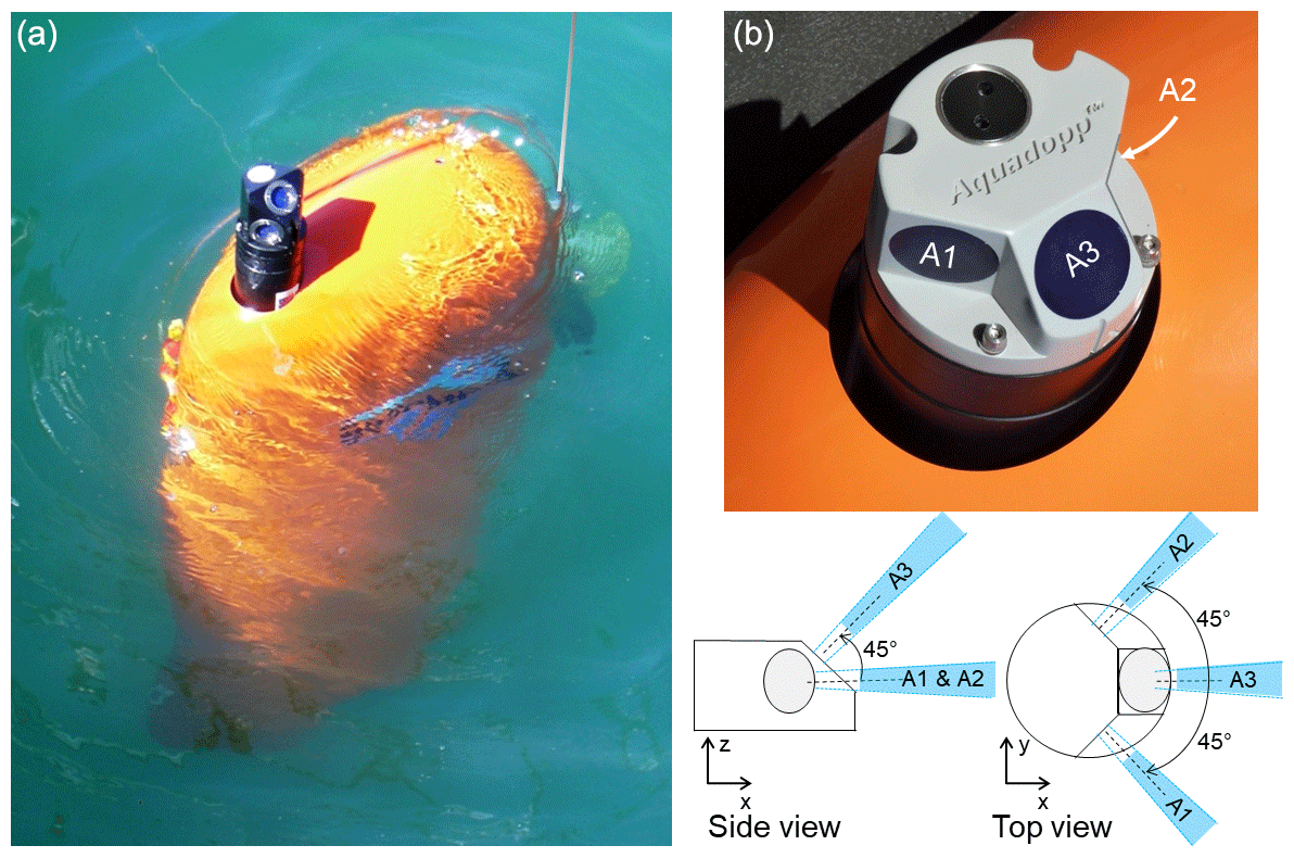
Figure 1The moored Aqualog automatic mobile profiler with a deep-water Aquadopp acoustic Doppler current meter (a). Transducer head of the shallow-water Aquadopp acoustic Doppler current meter on the Aqualog profiler (b). Bottom right: the acoustic beams are shown in blue and are labeled A1, A2, and A3.
This study is based on the comparative analysis of the amplitude of sound backscattering data at a frequency of 2 MHz and oxygen concentration data in seawater obtained in the NE Black Sea using a moored automatic mobile profiler, Aqualog (Fig. 1) (Ostrovskii and Zatsepin, 2011, 2016; Ostrovskii et al., 2013). To obtain the depth profiles of the volume backscattering strength, the Aqualog profiler was equipped with a Nortek Aquadopp acoustic Doppler current meter (https://www.nortekgroup.com/assets/documents/ComprehensiveManual_Oct2017_compressed.pdf, last access: 19 July 2021).
The Aquadopp is a narrow-band instrument (https://support.nortekgroup.com/hc/en-us/articles/360029839331-The-Comprehensive-Manual-ADCP, last access: 19 July 2021) that emits short sound pulses (pings) at a constant frequency and receives reflected (echo) signals. Plankton and suspended matter, as well as air and gas bubbles, are the main scatterers of the sound. While sound pulses are scattered in all directions when they hit particles, a small fraction of the incident sound pulse intensity is reflected. The Aquadopp current meter employs a mono-static system in which three transducers are used to transmit and receive signals at an acoustic frequency of 2 MHz. Measurements are made in the 90 dB range with a resolution of 0.45 dB. In high-accuracy acoustic Doppler measurements, the acoustic beams are narrow, and each has a cone angle of 1.7∘. Three focused beams measure the scattering strength with high sampling rates in a small volume (referred to as a single point). Two-sided acoustic beams are directed horizontally with 90∘ spacing between the axes of the beams (Fig. 1). These beams measure the volume scattering strength at the level of the transducer. The third beam is inclined at an angle of 45∘ to the plane formed by the axes of the other two beams. The piezoelectric element of the transducer transmits sound waves when it vibrates. The vibration does not stop at once but is damped over time. The speed of sound in water and the damping time of the membrane vibration determine the dead zone. In our case, this distance along the acoustic beam is approximately 0.35 m from the piezoelectric element of the transducer to the measurement cell (in the form of a truncated cone). The sound pulses are scattered and reflected back to the transducer. In our case, the length of the cell along the axis of the acoustic beam is approximately 1.5 m. Therefore, the reflected sound pulse intensity obtained by the instrument is the weight average for the time during which the sound wave passes the distance of 1.85 m to the far boundary of the measurement cell plus 1.85 m on the way back. The received signal is processed in such a way that the greatest contribution to the average value is made by the scattering in the center of the measurement cell at a distance of approximately 1.1 m from the transducer. The device can transmit up to 23 sound pulses every 1 s. The average value of the volume scattering strength for sound pulses transmitted and received in 1 s is recorded in the device's memory.
The high frequency of 2 MHz allows for observations of small-sized sound scatterers. Theoretically, a 2 MHz transducer is most sensitive to particles with a diameter of 0.23 mm (estimates for different frequencies for standard seawater are given, for example, in Hofmann and Peeters, 2013). However, this is not entirely applicable to zooplankton due to the complex shape of these organisms, their structure, their lipid composition, and the presence of gases in their bodies (Stanton et al., 1994; Lavery et al., 2007; Lawson et al., 2006). However, as a simplified model, copepod species are often considered cylinders, the scattering from which is defined as a function of the incident sound pressure, the acoustic wavelength, and the distance between the transmitter and the animal. An approximate formula for describing sound scattering from an elongated weakly scattering body of an animal also includes the angle of orientation of the body (Stanton et al., 1993, 1994). Unfortunately, the manufacturer of the Aquadopp instrument does not specify information about the acoustic power of its transducers. The Aquadopp measurement data for the volume scattering strength are presented in conventional units (counts). Without special calibration, it is not possible to determine the amount of falling sound pressure in water at a distance from the instrument transducer.
Since 2013, Aquadopp instruments with sideways-looking vertically mounted heads have been regularly used on the Aqualog profiling carrier (Fig. 1). The carrier moves up or down at a speed of approximately 0.2 m s−1, so the vertical resolution of the volume scattering strength data is 0.2 m. These data are averaged every 5 s, allowing for the detection of an SSL with a thickness on the order of 1 m.
In the context of this study, the ability to observe sound that has been reflected from zooplankton species at different angles is important. In the case of settling detritus, the volume scattering strength of slanted beam A3 and that of horizontal beams A1 or A2 are approximately the same. If the elongated suspended particles are oriented vertically or inclined, the amplitude of A3 will significantly differ from the amplitudes of A1 and A2. This was shown for copepods based on both models of acoustic scattering at a frequency of 2 MHz (Stanton and Chu, 2000; Roberts and Jaffe, 2007) and laboratory experiments (Roberts and Jaffe, 2008).
Thus, by comparing the amplitudes A1, A2, and A3, one can judge the predominant orientation of species in zooplankton aggregations. It is assumed that the aggregation's characteristic size is greater than the length of the acoustic measurement cell, that is, not less than ∼ 2 m, and its lifetime is longer than 10 s. Therefore, during the Aqualog carrier movement at a speed of 0.2 m s−1, the slanted and horizontal acoustic beams scan the same zooplankton aggregation. The complexity and variability of the acoustic backscatter makes it difficult to compare the acoustic signals obtained for different observational periods. Proper normalization of the signals is needed to evaluate the seasonal change in the vertical distribution of the mesozooplankton SSLs from many profiles despite the variability of the amplitude of the acoustic backscatter. For the Aquadopp instrument, such normalization is the ratio of the volume scattering strength of the horizontal beams to the volume scattering strength of the slanted beam:
It allows for a drastic reduction in the noise associated with clouds of sinking particles, which have an approximately equal area in the horizontal projection to the projection with a 45∘ angle of inclination. In some cases, the suspended particles can completely obscure the signal associated with the aggregation of mesozooplankton. However, in this study, there were usually only a few such cases. As will be shown below in Sect. 3, typically at depths from 60 to 120 m during the day, the directional acoustic backscatter ratio R = 1.05–1.2, and at night, R < 1.05. In the Appendix, we will consider whether the mesozooplankton specimens' vertical orientation is tilted in the deep aggregations. The analysis will be based on calculation of the ratio of the volume scattering strength of the horizontal beams , assuming that due to the tilt the standard deviation of should be greater than 0.
In addition to the Aquadopp instrument, a SeaBird 52MP CTD probe and Aanderaa 4330F and SBE 43F dissolved oxygen fast sensors were incorporated into the Aqualog profiler aerobic zone (Ostrovskii and Zatsepin, 2016). The SeaBird 52MP CTD was specially designed for a moored profiling application in which the instrument makes vertical profile measurements from a carrier that travels vertically beneath a subsurface floatation (https://www.seabird.com/sbe-52-mp-moored-profiler-ctd-optional-do-sensor/product-downloads?id=60762467706, last access: 19 July 2021). The CTD is equipped with a pump that controls a flow at a constant speed through a single small diameter opening to ensure the minimization of salinity spiking in the measurement data by the temperature and conductivity cell. On the Aqualog profiling carrier slowly moving at ∼ 0.2 m s−1, the CTD sampling rate of once per second provides sufficient data to resolve ocean fine-scale thermohaline structure. The accuracy of the CTD probe is 0.002 ∘C for the temperature, ± 0.0003 S m−1 for the conductivity, and ± 0.1 % of the full scale range for the pressure. The SBE 43F accuracy should be no worse than ± 2 % saturation, which can be compared with 5 % for Aanderaa 4330F with a resolution better than 1 µm or 0.4 % (https://www.aanderaa.com/media/pdfs/d378_aanderaa_oxygen_sensor_4330_4330f.pdf, last access: 19 July 2021). In practice, in the Black Sea, SBE 43F showed very robust results in detecting the lower boundary of the oxic zone, consistent with observations of the sigma-density structure and definition of the oxic zone boundary for the northeastern region of the Sea (Ostrovskii and Zatsepin, 2016). The SeaBird 52MP CTD with SBE 43F was regularly calibrated at the facility of the Southern Branch of the Shirshov Institute of Oceanology, Gelendzhik. The dissolved oxygen measurements using the Aanderaa 4330F and SBE 43F sensors at the profiler were described in Ostrovskii and Zatsepin (2016) and later in a companion paper (Ostrovskii et al., 2018). The fast-response sensing foils of the Aanderaa 4330F sensor were replaced by new foils two times in the past 4 years. The CTD and dissolved oxygen sensors were mounted at the leading edge of the Aqualog profiler pointing into horizontal oncoming flow, while hydrodynamic cowling (vertically oriented, wing-like) helped to stabilize the profiler orientation with respect to the flow direction. It should be noted that the Black Sea environment is particularly suitable for profiling measurements since there is no biological fouling on the sensors of the profiler, which is usually submerged into the hydrogen sulfide zone for ∼ 10 min every 1–2 h. Finally, the dissolved oxygen sensor data were verified with the water samples at standard depths for determination of dissolved oxygen by Winkler method (not shown here).

Figure 2The Black Sea coastline (https://osmdata.openstreetmap.de/data/coastlines.html, last access: 19 July 2021). The observational site off Gelendzhik is shown by a red dot. © OpenStreetMap contributors 2021. Distributed under the Open Data Commons Open Database License (ODbL) v1.0.
Table 1Deployments of the profiler Aqualog-6 with a Nortek Aquadopp current meter in the NE Black Sea and the dates of the zooplankton sampling near the profiler mooring site in 2010–2021. Since 2013, the profiler Aqualog has been equipped with a SBE 52MP CTD probe with a SBE 43F DO sensor. Additional sensors used on the profiler were as follows: Oxygen Aanderaa 4330F, Seapoint Turbidity Meter, and Seapoint Fluorometer. The unit “cpd” denotes the profiling cycles per day.
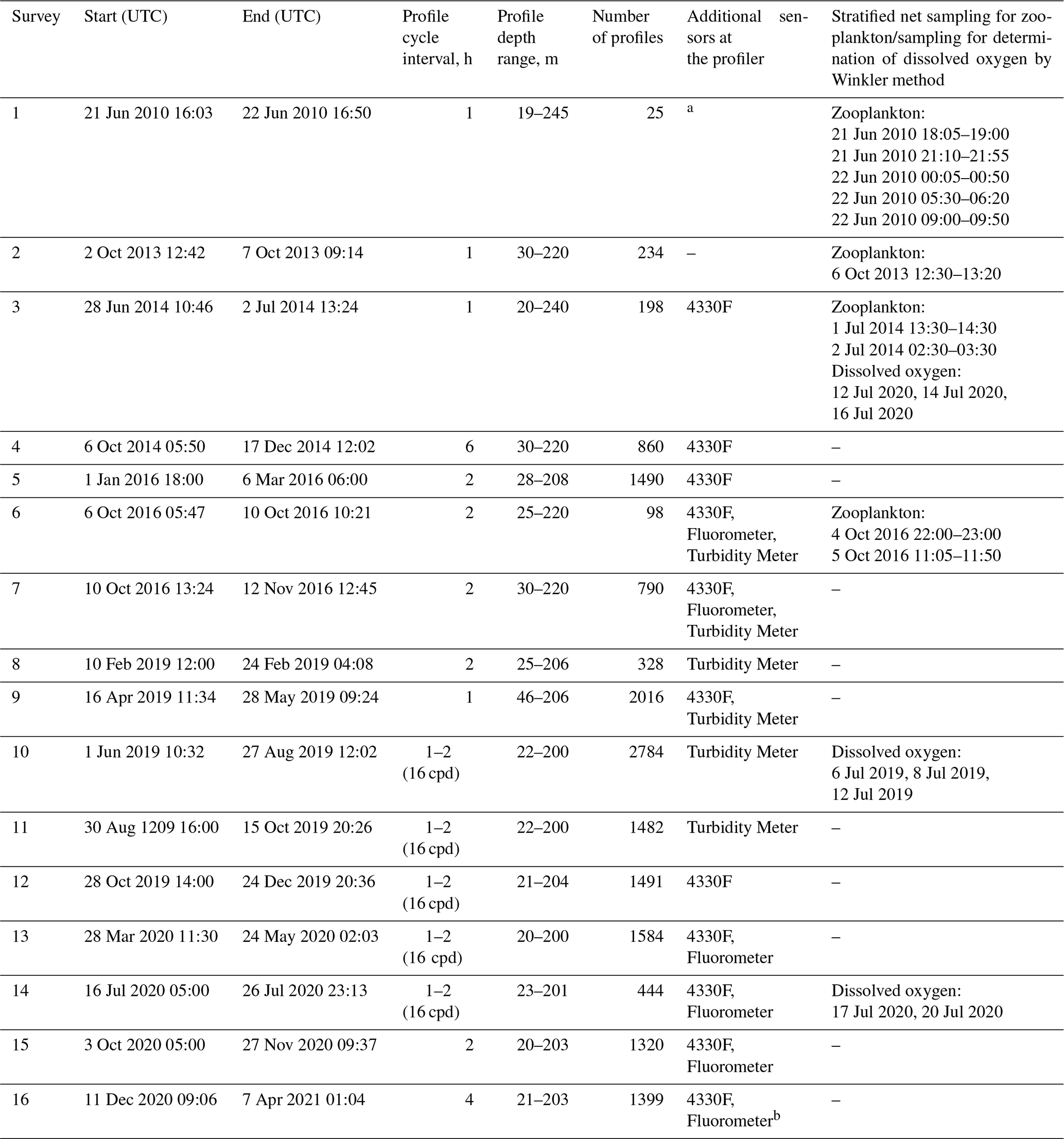
a No dissolved oxygen sensor. b Nortek Aquadopp broken.
The profiler mooring station was deployed approximately 4 nmi from the coast at the uppermost part of the continental slope at 44∘29.3′ N and 37∘58.7′ (Fig. 2). From June 2010 to April 2021, 16 surveys lasting from a few days to 3 months were carried out (Table 1) (Solovyev et al., 2021). During the surveys, the device automatically performed a profiling cycle usually every 1–2 h, descending to the near-bottom depth of 200–220 m and ascending to the upper layer while remaining submerged at a depth of 20–40 m. In particular, in 2016–2020, more than 14 000 multiparameter sets of vertical profiles were collected year-round (except March).
To acquire taxonomic and quantitative features of zooplankton vertical distribution, stratified net samples were taken from R/V Ashamba (Table 1) near the moored profiler Aqualog with a Juday net (mouth area 0.1 m2, mesh size 180 µm) equipped with a closing device. The towing speed was 0.9–1.0 m s−1, and the net was closed without stopping the upward movement. The sampling was carried out in calm weather so that the wire angle was not higher than 10∘. The sampling was carried out at earlier stages of this project in June 2010, October 2013, and July 2014, as well as later in October 2016.
The net hauls targeted the backscattering aggregation considering that their locations were associated with specific isopycnal layers (Ostrovskii and Zatsepin, 2011, Fig. 9). Vertical profiles of temperature, salinity, and density were obtained with a shipborne SeaBird 19plus CTD probe prior to mesozooplankton sampling. Depth strata were chosen based on the CTD profiles to sample the upper mixed layer (UML), the thermocline layer, the layer from the oxycline upper boundary (σΘ = 14.25) to the lower boundary of the thermocline, and two layers in the oxygen-deficient zone: the layer from depths of σΘ 15.7 to σΘ 15.4 and the layer from 2–3 m below σΘ 15.9 to σΘ 15.7.
The time of sampling corresponded to the day–night vertical distribution and upward–downward migration of zooplankton (June 2010), the daytime distribution (October 2013), and the day–night distribution (July 2014 and October 2016). The samples were immediately fixed with buffered formaldehyde (4 % final concentration of seawater–formaldehyde solution). The volume of filtered sea water was estimated from the area of the net mouth and the length of the released wire. Organisms were identified and counted under a stereomicroscope equipped with an ocular micrometer. Zooplankters were identified at the level of species and age stages of copepods and size classes (with an interval of 2 mm) of chaetognaths and ctenophores. The smallest organisms (meroplankton, appendicularians, copepod nauplii, and ova) considered in the analysis were 180 µm in size. Mesozooplankton biomass in terms of dry weight (DW) was estimated based on the published length–DW regressions for different species summarized in Arashkevich et al. (2014, Table 2). Biomass values were standardized to units of milligrams of dry weight per cubic meter (mg DW m−3) or milligrams of dry weight per square meter (mg DW m−2). The intensity of the echo signal strongly depends on the material properties of the organism's tissue (Stanton et al., 1994); therefore, when comparing the pattern of the scattering signal intensity with the pattern of zooplankton distribution in a community containing different taxa, it was reasonable to express zooplankton biomass as DW or carbon (Flagg and Smith, 1989; Heywood et al., 1991; Ashjian et al., 1998). For a graphical presentation of the results, six components of zooplankton were considered: copepods Calanus euxinus and Pseudocalanus elongatus, small crustaceans (Acartia clausi, Paracalanus parvus, Oithona similis and cladocerans), heterotrophic dinoflagellate Noctiluca scintillans, chaetognaths Parasagitta setosa, and varia (ctenophores Pleurobrachia pileus, appendicularians, meroplankton, decapod larvae, Pisces ova).
One method for calculating vertical migration speed of zooplankton from the sound backscatter data of the acoustic current meter at the profiler Aqualog was described in Pezacki et al. (2017). However, the vertical migration speed of mesozooplankton is beyond the focus of this study. Only once when discussing the pattern of the diel vertical migration is the slope of the migration track on the echogram (see Fig. 9 below) considered to give a rough idea about the dive and the ascent of mesozooplankton. Much more effort would certainly be needed to visualize the specimens' vertical swimming.

Figure 3Diurnal motions of the sound-scattering layers in the oxic zone. The depth–time scatterplot for profiles of acoustic backscatter amplitude at 2 MHz was obtained using the Aquadopp instrument at the moored profiler during verification study involving net sampling of zooplankton on 21 and 22 June 2010.
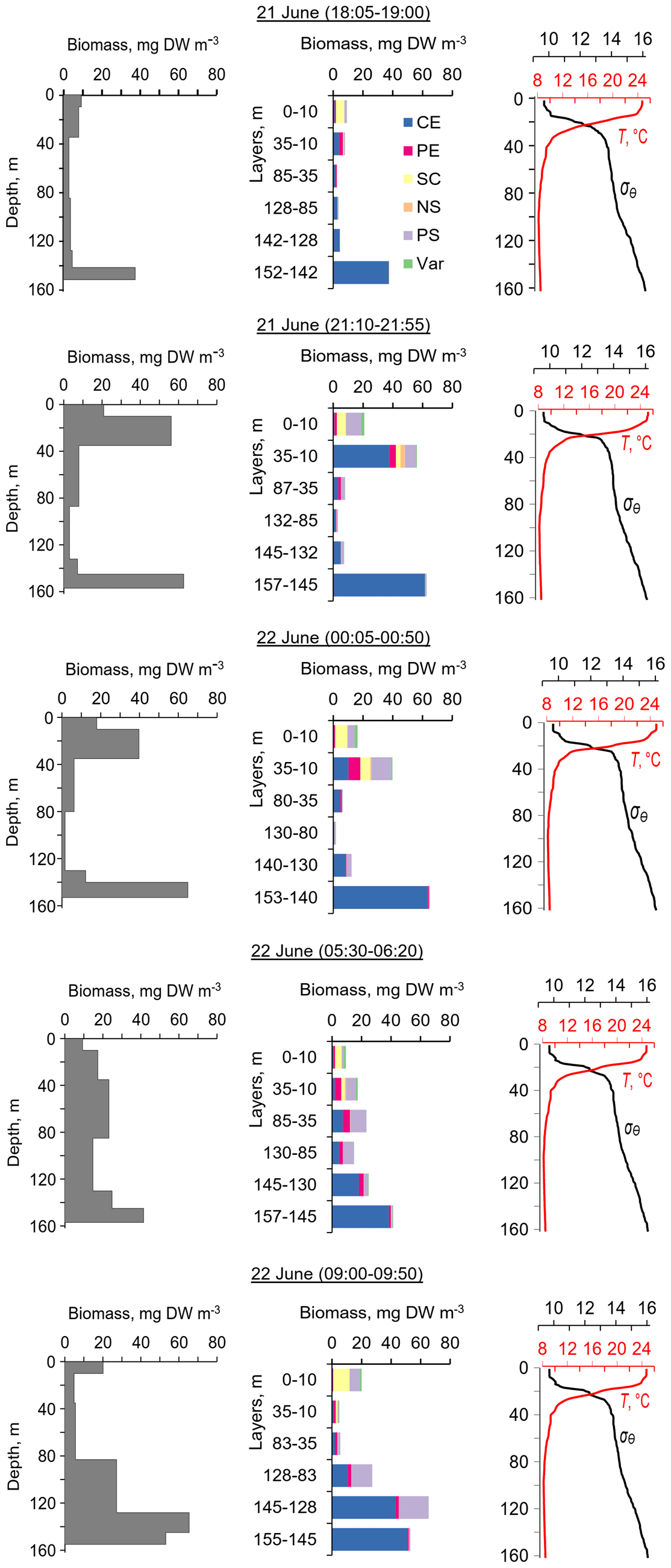
Figure 4The diel changes in vertical distributions of (left) total mesozooplankton biomass, (middle) zooplankton composition, and (right) temperature (T) and density (σΘ) near the mooring site on 21 and 22 June 2010. The temperature and density profiles were used for the selection of sampling strata. CE – Calanus euxinus; PE – Pseudocalanus elongatus; SC – small crustaceans; NS – Noctiluca scintillans; PE – Parasagitta setosa; Var – varia.
3.1 Acoustic scattering by mesozooplankton aggregations
The first validation data for the Aquadopp observations were obtained on 21 and 22. June 2010. The sound-scattering layers were identified at the raw echogram (Fig. 3) as mesozooplankton aggregations by comparison with the net sampling data (Fig. 4). The zooplankton net sampling data were consistent with the acoustic backscatter, indicating short-term variations in biomass and diel vertical migration of zooplankton.
The total mesozooplankton biomass in the entire water column varied from 0.99 to 3.57 g DW m−2. Zooplankton was dominated by the copepod Calanus euxinus, which made up the mean 58 % with the standard deviation (SD) ± 14 % of the total biomass (below for the sake of brevity, such estimates are denoted as mean ± SD%). The contribution of chaetognaths Parasagitta setosa was 21 ± 11 %, followed by copepods Pseudocalanus elongatus (13 ± 7 % of the total biomass). The sum share of other groups of mesozooplankton did not exceed 7 % of the total biomass.
The pattern of the vertical distribution of mesozooplankton biomass reveals a relatively uniform distribution over depth in the evening twilight (18:05–19:00) and at dawn (05:30–06:20) (Fig. 4, left column). At night (21:10–21:55 and 00:05–00:50), the highest concentration of zooplankton was observed in the thermocline layer, while in the daytime (09:00–09:50), the zooplankton maximum was in the layer between the density surfaces σΘ 15.7 and 15.4 (Fig. 4, left column), in accordance with the diurnal changes in the volume backscatter strength (Fig. 3). The deepest layer bounded by isopycnals σΘ 15.9 and 15.7 was inhabited by nonmigrating copepods, the fifth copepodite stage (CV) of C. euxinus (median prosome length 2.3 mm), persistently staying at this depth throughout the day (Figs. 3 and 4, middle column). Visual inspection of live samples revealed quiescent behavior of these specimens and large oil sac volume inside their body, suggesting a diapausing state in C. euxinus CV collected from the deepest layer (Vinogradov et al., 1992).
Three migrating species, copepodites CIV–CVI of C. euxinus (median prosome length 2.6 mm), CV–CVI P. elongatus (median prosome length 0.92 mm), and chaetognaths P. setosa (median length 19 mm), formed daytime zooplankton aggregations in the oxygen-deficient zone (Fig. 4, middle column). Ctenophore Pleurobrachia pileus, also inhabiting the deep layers in the daytime, contributed negligibly to the total biomass due to the low dry matter content in their gelatinous bodies and their low abundance (shown as Var in Fig. 4). At night, most of the migrating zooplankters were concentrated in the thermocline and did not ascend to the warm UML, which was inhabited by small copepods, cladocerans, and small (< 6 mm) chaetognaths.
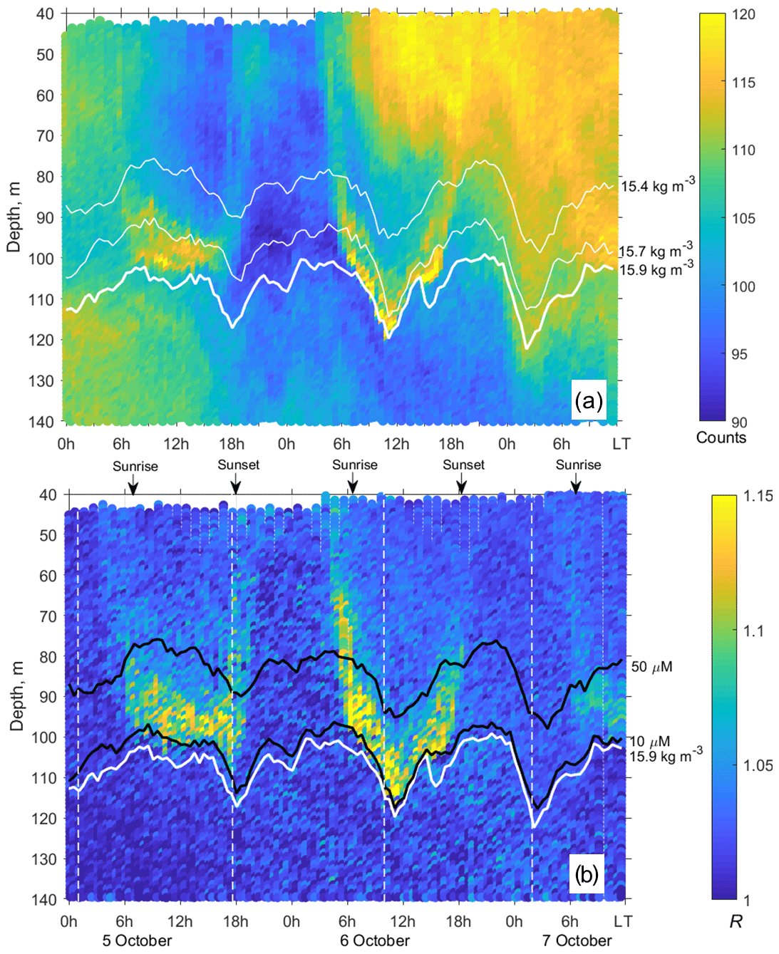
Figure 5(a) The time–depth graph of the Aquadopp horizontal-beam echogram showing acoustic backscatter intensity (counts) on 5–7 October 2013. The Aqualog profiler with the Aquadopp instrument performed ascending–descending cycles every 1 h. The upper, middle, and lower white lines are for isopycnals σΘ 15.4, 15.7, and 15.9, respectively. (b) Time–depth scatterplot of the Aquadopp directional acoustic backscatter ratio R = . Colored lines show [O2] = 50 µm (upper black line); [O2] = 10 µm (lower black line); and σΘ = 15.9 kg m−3 (white line), which can be taken as a proxy for the boundary of the oxygen zone in the NE Black Sea (Glazer et al., 2006, Ostrovskii and Zatsepin, 2016). Notice that due to upwelling, the oxycline was moved upward. Vertical dotted white lines indicate a 17.3 h time interval, which is equal to the period of inertial oscillations at the latitude of the observation. They approximately coincide with troughs of inertial waves.
3.2 Zooplankton aggregations visualized using the directional acoustic backscatter ratio
The echograms based on the data from horizontal-beam transducers A1 and A2 often reveal aggregations of zooplankton at depths of 80–120 m in the daytime (Fig. 5). The aggregations begin to rise around sunset and descend before dawn. Thin, nearly vertical lines on the echogram indicate acoustic traces of the migrating mesozooplankton species. The echogram also shows patches that occupy the entire water column, from the upper to the lower measurement depth, penetrating below the surface σΘ 15.9 and then deeper into the hydrogen sulfide zone. These are clouds of suspended particles (see, for example, Klyuvitkin et al., 2016). Acoustic scattering by clouds of particles sinking through the water column can obscure zooplankton aggregations.
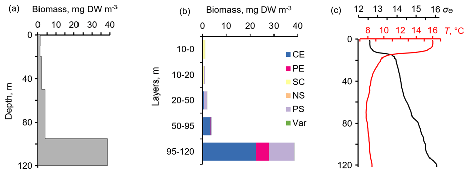
Figure 6The daytime vertical distributions of (a) total mesozooplankton biomass, (b) zooplankton composition, and (c) temperature (T) and density (σΘ) near the mooring site at 12:30–13:20 on 6 October 2013. Temperature and density profiles (c) indicate the selection of sampling strata. CE – Calanus euxinus; PE – Pseudocalanus elongatus; SC – small crustaceans; NS – Noctiluca scintillans; PE – Parasagitta setosa; Var – varia.
The layers of elevated acoustic backscatter amplitude due to deep zooplankton aggregations are accounted for using the R graphs (Fig. 5b) that were validated by net sampling on 6 October 2013 (Fig. 6), although sampling was not performed at night due to stormy weather. Since the depths of the isopycnals of 15.9 and 15.7 differed by only 3 m, the integrated zooplankton sample was taken in the layer between σΘ = 15.9 and σΘ = 15.4. In this layer, the contributions of Calanus euxinus, Parasagitta setosa, and Pseudocalanus elongatus to the total biomass were 60 %, 26 %, and 12 %, respectively (Fig. 6b). The extremely low zooplankton biomass (< 2 mg DW m−3) in the upper 50 m layer (Fig. 6a and b) is consistent with data on a 4-fold decrease in the annual average biomass of upper dwelling zooplankton in 2013 compared to previous years (Arashkevich et al., 2015).
Zooplankton diel vertical migration trajectories in the R graph are noticeably clear below 40 m (Fig. 5b). The explanation of these phenomena could be that the scattering area of the elongated bodies of the zooplankton species is larger in the horizontal projection than in the inclined projection at an angle of 45∘. Therefore, the orientation of the bodies of mesozooplankton species appears to be mainly vertical during migration. At night, these specimens are randomly oriented in the upper layer, where R≈1. In addition to the diel vertical migrations, intraday vertical fluctuations of zooplankton occur with an inertial period (Fig. 5b). The vertical displacements of the daytime deep mesozooplankton aggregations are coherent with the vertical displacements of both isopycnals and isooxylines. The displacements of isopycnals with amplitudes up to 20 m are mainly due to near-inertial waves.

Figure 7(a) The time–depth scatterplot of the Aquadopp horizontal-beam echo on 6–10 October 2016. (b) The time–depth graph of the Aquadopp directional acoustic backscatter ratio R. The isopycnals and isooxylines are superimposed near the SSLs.
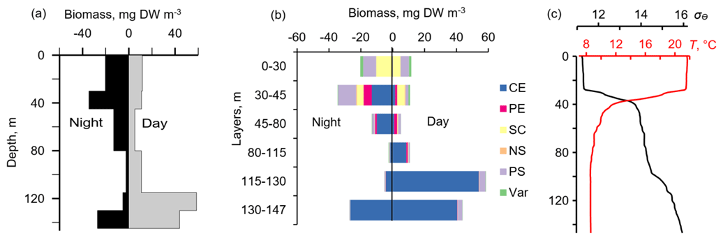
Figure 8Day–night vertical distribution of (a) total mesozooplankton biomass, (b) zooplankton composition, and (c) temperature (T, ∘C) and density (σΘ) near the mooring site at 22:00–23:00 on 4 October (night) and 11:05–11:50 on 5 October (day) 2016. Temperature and density profiles (c) indicate the selection of sampling strata. CE – Calanus euxinus; PE – Pseudocalanus elongatus; SC – small crustaceans; NS – Noctiluca scintillans; PE – Parasagitta setosa; Var – varia.
In October 2016, persistent aggregation of diapausing C. euxinus was detected in the acoustic backscatter signal (Fig. 7), unlike October 2013 (Fig. 5). Zooplankton sampling was performed at midnight and midday on 4 and 5 October 2016 (Fig. 8). The pattern of zooplankton distribution was similar to that in June 2010 (Fig. 4), both in terms of the total biomass and composition of zooplankton and in terms of the day–night vertical distribution. The total mesozooplankton biomass of 1.8–2.3 g DW m−2 was dominated by three species: C. euxinus (59 %–76 %), P. setosa (9 %–22 %), and P. elongatus (5 %–10 %). At night, the maximum aggregation of migrating zooplankters was in the thermocline layer, and at midday, it was in the layer between isopycnals σΘ 15.7 and 15.4 (Fig. 8a). Daytime zooplankton aggregation consisted mainly of C. euxinus (92 % of total biomass) with a small contribution from chaetognaths (7 % of total biomass) (Fig. 5b). The layer between isopycnals σΘ 15.9 and 15.7 was persistently occupied by diapausing C. euxinus CVs. The chaetognaths found in this layer were represented by spent specimens and corpses (Fig. 8b). UML was inhabited by nonmigrating small copepods, cladocerans, and small chaetognaths.
The net sampling data on the day–night vertical distribution of mesozooplankton agreed broadly with the acoustic backscatter observations obtained during the next few days (Fig. 7). On the echogram, one can see a persistently existing backscattering layer associated with the isopycnal layer near σΘ = 15.9, as well as patches of the high-volume backscattering strength at depth during the daytime and their movement into shallower layers at night.
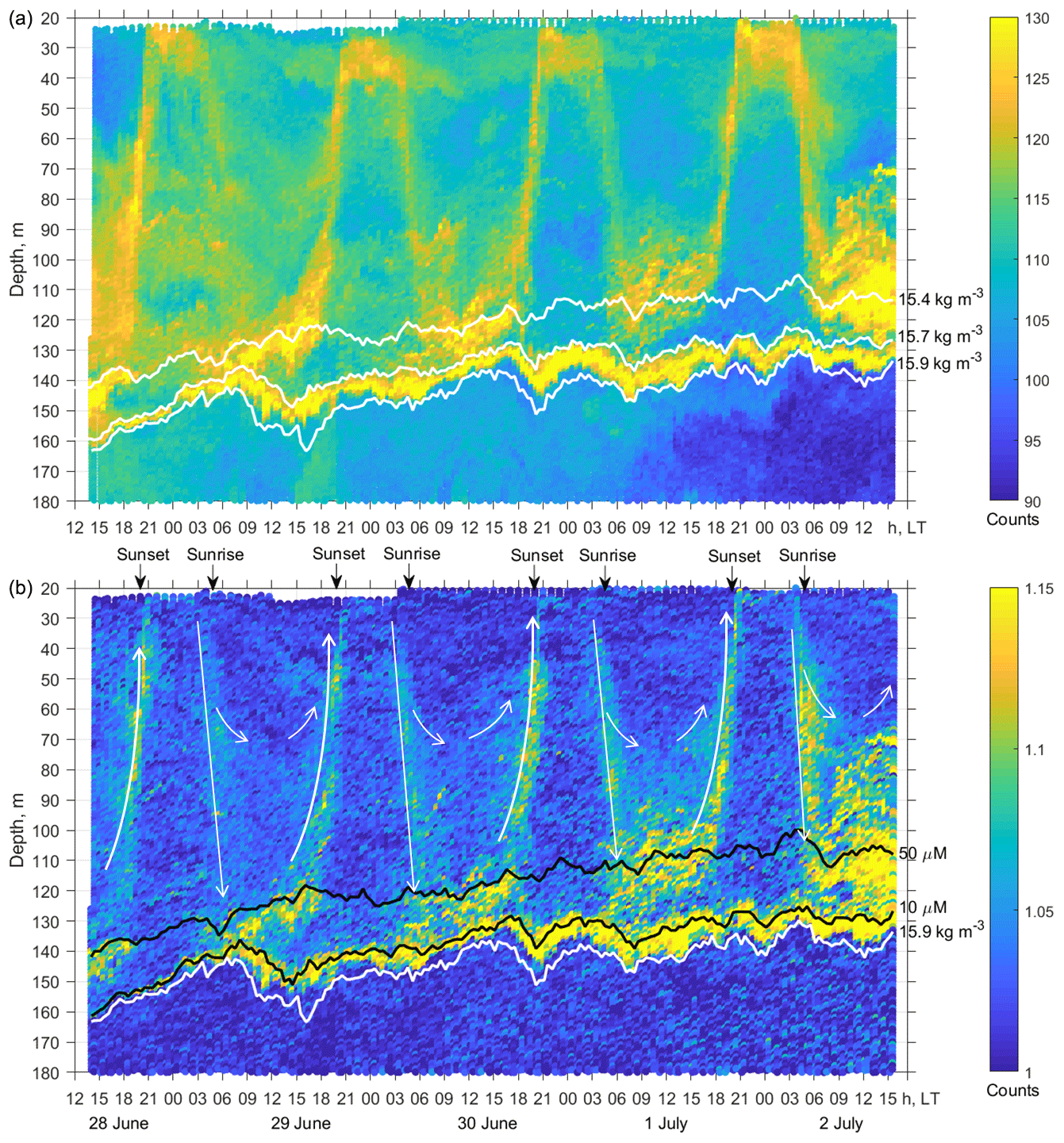
Figure 9(a) The time–depth graph of the Aquadopp horizontal-beam echo during the moored profiler survey on 28 June–2 July 2014. The isopycnals are superimposed near the SSLs. (b) The graph of time–depth variation in R based on the measurements of sound backscattering. The upper and lower black lines are isooxylines of 50 and 10 µm, respectively. The white line indicates isopycnal σΘ = 15.9. There is a persistent SSL under isooxyline [O2] = 10 µm. Thin white arrows schematically show the diel migration of mesozooplankton. The maximum depth of the diel vertical migration is 120–150 m, although some specimens dive to depths of only 80–100 m. The slope of the straight arrow pointing downwards corresponds to a diving speed of ∼ 1.5 cm s−1. The ascent is accelerated and reaches values of approximately 2.5 cm s−1 in the upper 60 m depth.
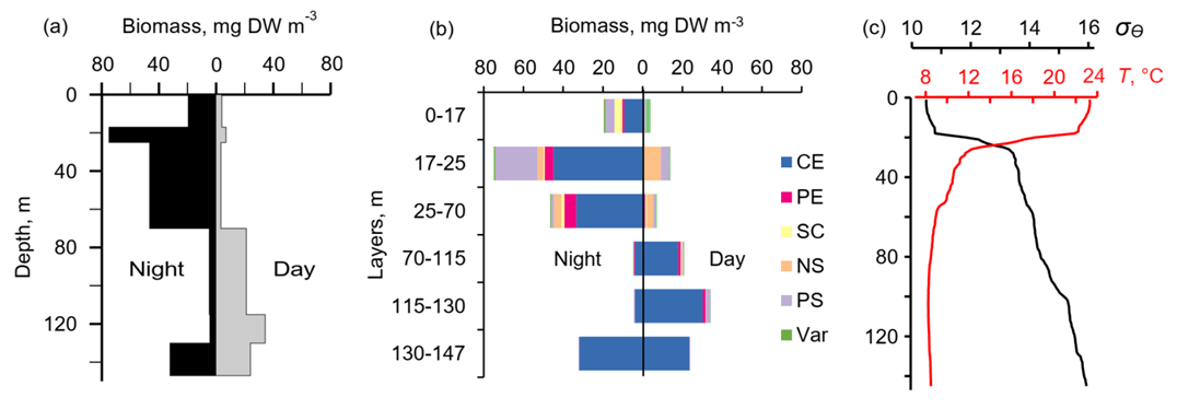
Figure 10The day–night vertical distribution of (a) total mesozooplankton biomass, (b) zooplankton composition, and (c) temperature (T) and density (σΘ) near the mooring site on 1 July (13:30–14:30) and 2 July (02:30–03:30) 2014. Temperature and density profiles (c) indicate the selection of sampling strata. CE – Calanus euxinus; PE – Pseudocalanus elongatus; SC – small crustaceans; NS – Noctiluca scintillans; PE – Parasagitta setosa; Var – varia.
The two-layered structure was also observed at the end of June–early July 2014 (Fig. 9) and validated by day–night zooplankton sampling on 1 and 2 July (Fig. 10). Deeper zooplankton aggregation was monospecific, consisting only of diapausing C. euxinus CVs (Fig. 10b) and formed a thin layer (5–10 m thick). This layer was visible all day and night and was usually located above the isopycnal surface of 15.9. It is clearly distinguished by the value R > 1.1 (Fig. 9b). The daytime zooplankton aggregation consisted of three migrating species and their different developmental stages, C. euxinus, CIV–CVIs, P. elongatus, CV–CVIs, and P. setosa, 14–22 mm in size (Fig. 10b). Since the amplitude of vertical migration is different for different components of this assembly, the daytime deep aggregation reached 35 m in thickness. Before sunset, migrating zooplankters began to move upward and at night formed aggregations at depths above 40 m (Fig. 9a) and peaked in the thermocline at 17–25 m (Fig. 10a).
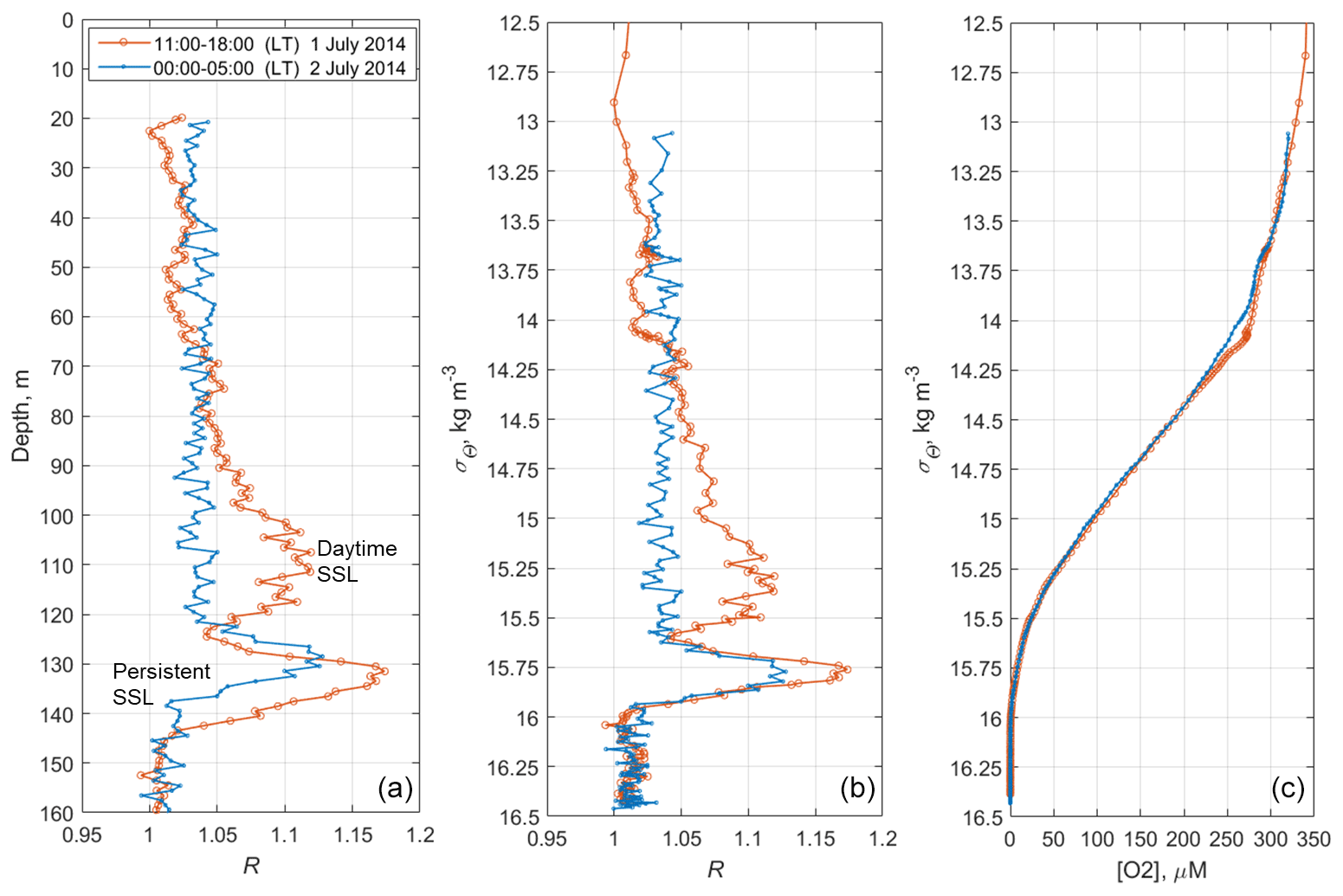
Figure 11The time averages of R and [O2] for the daytime of 1 July 2014 (red) and the nighttime of 2 July 2014 (blue), when net sampling (Fig. 10) took place. (a) The depth profiles of the time averages R. (b) The daytime and nighttime averages R vs. the specific density, σΘ. (c) Distribution of the daytime and nighttime averages of the dissolved oxygen concentration vs. σΘ.
Since migrating zooplankton aggregations were observed in the deep layers only during the daytime, it is worth comparing the daytime average R profile with that for the nighttime (Fig. 11). Such a comparison clearly reveals the deep maximum of R at the daytime migration depths of mesozooplankton at 90–120 m, as well as the persistent maximum of the diapause layer within the deeper layer at 125–140 m. Notably, the depths of the persistent SSL change by approximately 5 m from night to the daytime, while they completely overlap when considered vs. the density. Such variations in the depth of the SSL might be linked to inertial oscillations (Ostrovskii et al., 2018).
3.3 The seasonal variation in mesozooplankton dynamics in relation to dissolved oxygen concentration
In Sect. 3.2, it was shown that the mesozooplankton species float on isopycnals in the lower part of the oxycline and in the hypoxic zone. Both the diapausing aggregations and the daytime aggregations are displaced coherently by near-inertial waves. The deep aggregations of mesozooplankton are bounded by certain isopycnal surfaces and isooxylines.
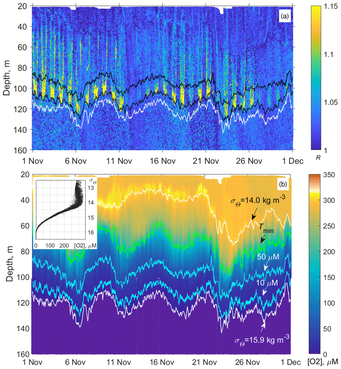
Figure 12(a) Example of the monthly long time series of the vertical profiles of the directional acoustic backscatter ratio R for November 2019 (in total 960 profiles from the moored profiler survey). The upper and lower black lines are isooxylines of 50 and 10 µm, respectively. The white line indicates isopycnal σΘ = 15.9. (b) Evolution of the dissolved oxygen at the profiler mooring site in November 2019. The colored lines indicate the following: the depths of the isopycnals σΘ = 14 and 15.9 (top and bottom white lines); the depth of the temperature minimum (green line); and [O2] = 50 and 10 µm (blue lines). The inset shows the diagram of the concentration of dissolved oxygen vs. the potential density, [O2] − σΘ, plotted from the moored profiler data of November 2019. In this example, as well as for other observational periods, the concentration of dissolved oxygen deviates very little from isopycnal surfaces in the lower part of the oxycline where [O2] < 200 µm.
Since the oxygen stratification strongly depends on the density stratification in the pycnocline (e.g., Vinogradov and Nalbandov, 1990; Codispoti, et al., 1991; Konovalov et al., 2005; see also example in Fig. 12), it becomes possible to switch from the depth profiles of the directional acoustic backscatter ratio R(z), where z is the depth, to the R([O2]) profiles to investigate the seasonal changes of the sound-scattering mesozooplankton layers in terms of R vs. [O2].
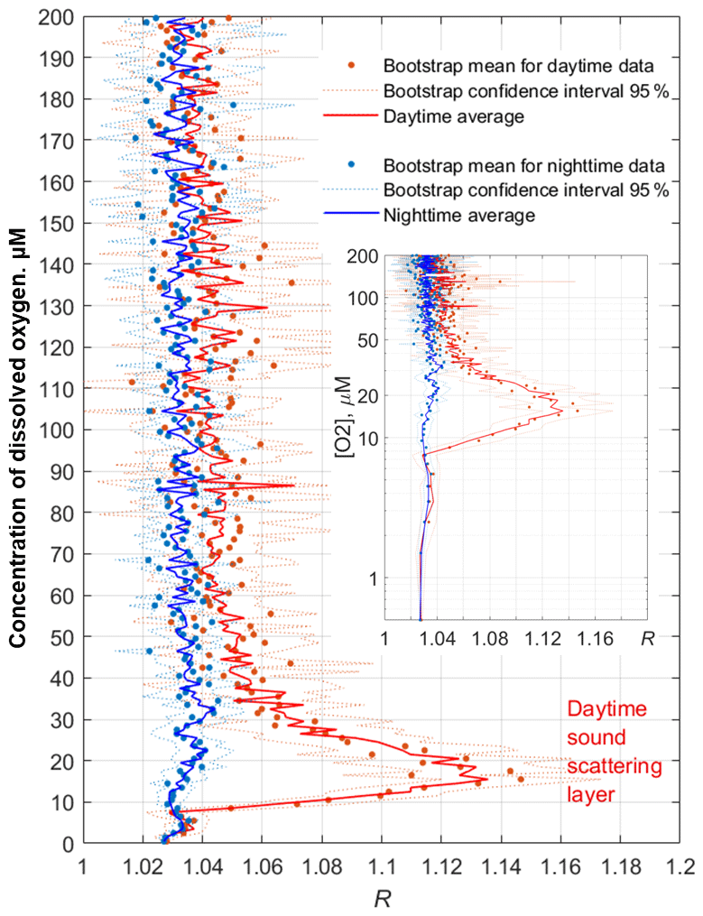
Figure 13Example profiles of the daytime and nighttime averages 〈R([O2])〉 in November 2019. The inset shows the same plots with the y axis drawn logarithmically to reflect the lower parts of the profiles (the hypoxic zone) in more detail.
The average monthly profiles of R([O2]) were constructed from R(z) and [O2](z) data for every month when the data were available. To compute the averages, the daytime was defined as a period beginning 2 h after the local time of sunrise (at a given date) and ending 2 h before sunset. The nighttime was defined as a period beginning 1 h after sunset and ending 1 h before sunrise. Example plots of the average profiles 〈R([O2])〉 computed as arithmetic and bootstrap mean values along with 95 % bootstrap confidence intervals are shown for November 2019 in Fig. 13. In the hypoxic zone, the average values 〈R([O2])〉 for the daytime are significantly higher than those for the nighttime. The daytime averages 〈R([O2])〉 > 1.06 were in the range of [O2] = 9–40 µm in November 2019.
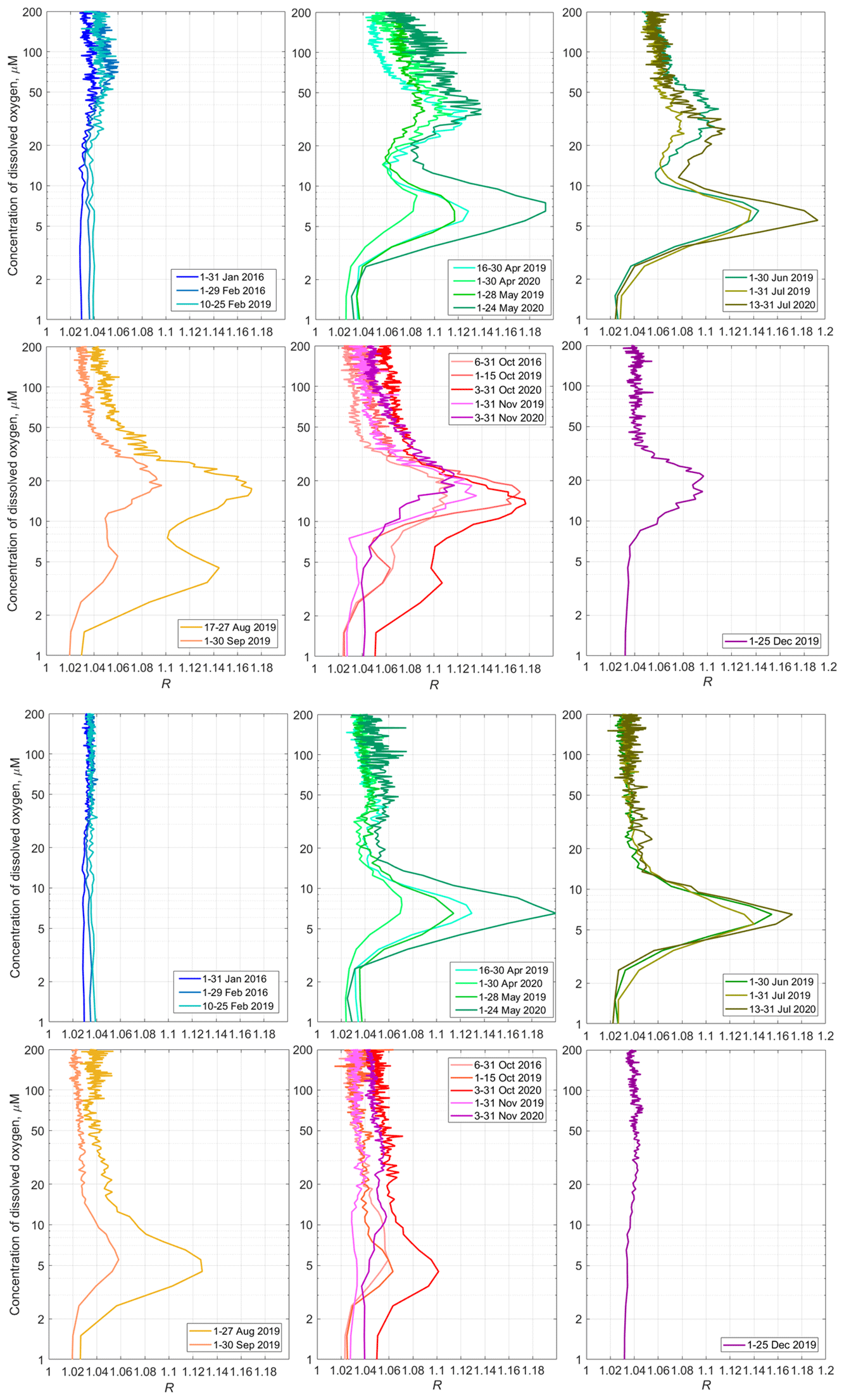
Figure 14Top – the monthly averaged profiles of 〈R([O2])〉 for the daytime over the upper part of the continental slope near Gelendzhik in the NE Black Sea. Bottom – the same for the nighttime.
The average monthly 〈R([O2])〉 profiles show the seasonal evolution of the mesozooplankton distribution (Fig. 14). The SSLs are barely discernible in January. One can note some activity in the upper part of the oxycline in February. Although we unfortunately do not have data for March, in April, two peaks appear in the 〈R([O2])〉 profiles in the layers where the concentration of dissolved oxygen is 25–60 µm and 4–9 µm. These maxima correspond to the daytime mesozooplankton aggregations and the diapause layer, respectively. The upper maximum of 〈R([O2])〉, which corresponds to the daytime aggregations of mesozooplankton, may weaken in June–July. However, it becomes stronger again at the end of summer and in autumn. The largest value for this maximum over the entire observation period 〈R([O2])〉 = 1.18 is observed in October. At that time, the maximum shifts into the layer where [O2] is 10–25 µm. In December 2019, this peak was between the 10 and 30 µm isooxylines.
The maximum of diapause mesozooplankton was strongest in May and July 2020, reaching almost 1.2 at [O2] = 5–8 µm. In August, the diapause mesozooplankton layer shifts in the lower part of the suboxic zone where [O2] = 3–7 µm. It becomes substantially weaker in September. In October, this layer degrades further. In November, it tends to disappear.
4.1 Visualization of the sound-scattering mesozooplankton aggregations
Previously, acoustic measurements at a frequency of 2 MHz were not considered a tool for observations of the mesozooplankton SSLs in the sea due to the limited range of soundings. However, with the advent of ocean profilers with acoustic Doppler current meters, such as the Nortek Aquadopp, it has become possible to obtain the depth profiles of the volume scattering strength at 2 MHz frequency in the entire water column and to study the vertical distribution of zooplankton, such as those in the Black Sea (Ostrovskii and Zatsepin, 2011; Pezacki et al., 2017). Acoustic sounding of mesozooplankton at two angles is made possible using the side-looking head of the Nortek Aquadopp instrument. The combination of horizontal and tilted beam signals allows, on the one hand, the patches of particles to be eliminated and the background scattering level of the echogram to be equalized and, on the other hand, the preferred orientation of mesozooplankton species migrating through the oxycline to be determined. Earlier, Stanton and Chu (2000) reproduced the influence of the orientation of a 3 mm calanoid copepod (modeled as a high-resolution approximation of an animal profile) on the acoustic target strength at 2 MHz with respect to an incident sonar beam. The reduction was found to be 5 %–15 % when copepod orientation was shifted from 0∘ (broadside incidence) to 30–60∘. Benfield et al. (2000) carried out field observations using the Video Plankton Recorder on George Bank and showed that most Calanus finmarchicus (75 %) in the depth range of 10–70 m were within ± 30∘ of the prosome-up or prosome-down orientation. It was suggested that one reason for the behavior underlying the head-up orientation pattern might be due to the predator avoidance strategy aimed at reducing the conspicuousness of C. finmarchicus when viewed from above. Such individuals would present a significantly reduced cross-sectional area to an echo-sounder's transducer with correspondingly diminished target strength. It was concluded that it is necessary to know how the orientation of individuals changes with depth to correctly account for the biomass of mesozooplankton. Experiments using a multiple-angle acoustic receiver array on live copepods and mysids in a laboratory tank showed that it is possible to use the scattered acoustic signal to distinguish among zooplankton taxa (Roberts and Jaffe, 2008). Reflections in the frequency range from 1.5 to 2.5 MHz were recorded from untethered 1–4 mm calanoid copepods and 8–12 mm mysids over an angular range of 0–47∘. That study demonstrated the utility of a multiple-angle acoustic array for zooplankton identification.
To distinguish the SSLs against the background patterns of vertical flow of settling particles and to study the orientation of zooplankton species, we propose a simple method for the processing of ultrasound sensing data at three angles. This acoustic three-beam geometry provides a partial pragmatic solution for the quest towards the multiple-angle scatter measurements suggested by models (Stanton and Chu, 2000; Roberts and Jaffe, 2007) and laboratory experiments (Roberts and Jaffe, 2008). Since the late 1990s, researchers' efforts have been focused on creating multichannel instruments to measure acoustic backscatter (volume scattering strength) at several frequencies, which contain information about the size composition of the scatterers, since different frequencies bounce off objects of different sizes (Wiebe et al., 2002; Smeti et al., 2015). Multichannel instruments in conjunction with video cameras are fairly expensive systems that are used for the identification of mesozooplankton in its natural habitat. Plausibly, a multichannel three-angle system featuring several relatively cheap short-range three-beam acoustic units each operating at an individual frequency when installed on a vertically profiling carrier would be a very effective tool for visualizing zooplankton aggregations.
4.2 The SSLs validated from the stratified net sampling
Comparison of the Nortek Aquadopp acoustic backscatter observations with the data obtained by stratified zooplankton sampling showed good agreement of the features of the diel vertical distribution of zooplankton. This was made possible by sampling narrow depth strata (10–15 m layers) targeting deep-water aggregations visualized on the echograms. The two-layered structure of the aggregations seen on echograms and R graphs in the daytime (Figs. 3, 7, and 9) reflected the species composition of zooplankton in these layers (Figs. 4, 8, and 10). The deepest layer bounded by isopycnals 15.9 and 15.7 was visible in the suboxic zone all day and night and was formed by diapausing CV Calanus euxinus. To some extent, this monospecific layer was contaminated by crustacean exuviae and carcasses, spent females, and zooplankters' remains sinking from the upper layers and apparently retained on the density gradient. The existence of a nonmigrating diapausing stock located in the suboxic layer from mid-spring to mid-autumn is confirmed by observations from submersible Argus (Vinogradov et al., 1985; Flint 1989), by high vertical resolution sampling with 150 L water bottles (Vinogradov et al., 1992), and by zooplankton net sampling (Arashkevich et al., 1998; Besiktepe, 2001; Svetlichny et al., 2009). However, for some unknown reasons, this nonmigrating layer was not detected by shipborne echo sounders at frequencies of 38–200 kHz (Erkan and Gücü, 1998; Mutlu, 2003, 2007; Stefanova and Marinova, 2015; Sakınan and Gücü, 2016), unlike our data obtained by Aquadopp at a frequency of 2 MHz.
The inclusion of diapause (or dormant stage) in the life cycle of all Calanidae species living in high-latitude and temperate environments is well known (e.g., see review in Baumgartner and Tarrant, 2017). Having accumulated a large amount of lipids, diapausing copepods descend into deeper ocean layers, where they can exist for several months at the expense of energy reserves. Decreased metabolic rate and developmental delay are characteristic features of diapausing copepods. In the Black Sea, a decrease in the metabolic rate in diapausing C. euxinus is caused not only by internal physiological reasons, but also by hypoxia in their dormant layer. The oxygen consumption rate in diapausing CV C. euxinus in hypoxia decreases by almost an order of magnitude, and the rate of ammonia excretion decreases 6 times compared with those in their active counterparts in normoxia (Svetlichny et al., 1998).
During the daytime, the upper SSL mostly located above σΘ = 15.7 consisted of four species, copepods C. euxinus and Pseudocalanus elongatus, chaetognaths Parasagitta setosa, and ctenophores Pleurobrachia pileus; the latter had a negligible contribution to dry biomass. This assembly had a wide range of body lengths from approximately 1 mm in P. elongatus to 22 mm in P. setosa. The different species had different swimming speeds. It was also possible that these species had different physiological tolerances to oxygen deficiency. This confirms earlier observations from the manned submersible, which showed that the daytime aggregation of migrating zooplankton had a layered structure: the lower layer was formed by chaetognaths, whereas the older stages of C. euxinus were located above, and ctenophores inhabited the upper part of the aggregation (Vinogradov et al., 1985; Flint, 1989). Furthermore, the different developmental stages of copepods C. euxinus and P. elongatus occupied different depths, deepening as their size increased (Morozov et al., 2019).
In the evening, approximately 2 h before sunset, zooplankters begin to ascend to the upper layers, where they spend all the dark hours concentrating in the thermocline layer and below it. In this layer, while feeding, they move in different directions and are oriented randomly (Kiørboe et al., 2009), so they cannot be discernible in the R graphs. According to our data, cold-water herbivorous C. euxinus and P. elongatus only occasionally ascend into the warm UML, mainly inhabiting colder layers rich in phytoplankton (see also the supplement to the paper by Morozov et al., 2019). Predator chaetognaths P. setosa move upward following copepods, their main prey (Drits and Utkina, 1988). The time of zooplankton migration clearly visible on the echograms is confirmed by the results of net sampling and is consistent with other published data (see for reference the Supplement of Morozov et al., 2019).
The vertical migration of zooplankton can increase the vertical flow of carbon and thus contribute to the functioning of the biological pump in the ocean (Tutasi and Escribano, 2020). The mesozooplankton that feed at the surface but metabolize and excrete at depth contribute to the transport of organic matter; more quantitatively, this contribution is estimated to be between approximately 10 %–50 % of the local sinking flux of organic particles (Bianchi et al., 2013, and references therein).
In the lower part of the oxic zone, the vertical displacements of SSLs coincide with the oscillations of isopycnal surfaces (Figs. 5 and 10). The dissolved oxygen concentration profile tightly hinges on the density stratification in the Black Sea since both are basically due to vertical mixing processes (e.g., Ostrovskii et al., 2018). Hence, displacements of the SSLs with regard to the oxy-isolines are much smaller than those vs. the depths. The vertical oscillations with a period of approximately 17 h near the mooring site are due to near-inertial waves (Ostrovskii et al., 2018). Irregular changes in isopycnal depths occur due to hydrodynamic events, such as individual internal waves, oceanic fronts, and jets. Occasionally, the isopycnal depth may change by 30–40 m within a day (Ostrovskii and Zastsepin, 2016).
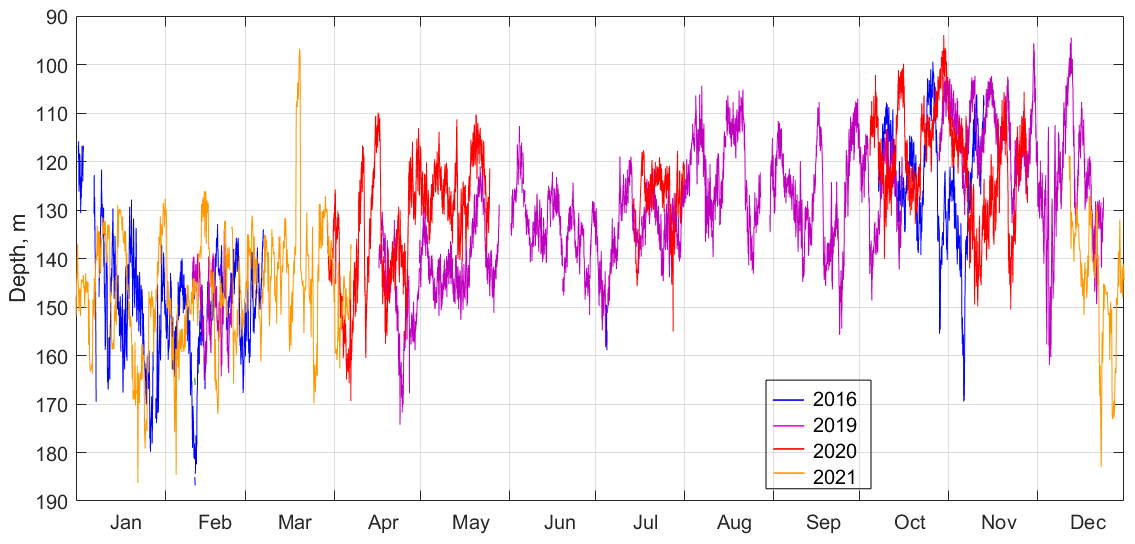
Figure 15The suboxic boundary depth ([O2] = 10 µm) as observed by the moored profiler in 2016, 2019, 2020, and 2021.
It is unlikely that copepods maintain their positions on certain isopycnal surfaces by swimming, as displacements of such large amplitudes by tens of meters require an additional depletion of energy reserves. A more beneficial strategy would be to adjust their buoyancy to neutral. Having neutral buoyancy in the hypoxic zone, the copepods would not need to spend much additional energy floating up and down following crests and troughs of internal waves while avoiding entrainment into the suboxic layer. Indeed, direct observations from manned submersibles revealed a quiescent behavior of diapausing copepods and their slow response to light and noise produced by underwater vehicles, both in the Santa Barbara Basin (Alldredge et al., 1984) and in the Black Sea (Mikhail Flint, personal communication, 2020). Neutral buoyancy has been hypothesized to be regulated by changes in lipid composition (Visser and Jónasdóttir, 1999); however, Campbell and Dower (2003) argued that this buoyancy regulation mechanism is inherently unstable because wax esters are more compressible than seawater. An alternative mechanism for buoyancy regulation in diapausing copepods that involves the replacement of heavy ions with lighter ammonium ions in hemolymph has been proposed by Sartoris et al. (2010) by analogy with other invertebrates. Later, Schründer et al. (2013) found high concentrations of ammonium ions in the hemolymph of a diapausing species, Calanoides acutus, and suggested that these copepods could achieve neutral buoyancy through their biochemical body composition without swimming movements. This mechanism obviously would better explain the observed phenomenon of diapausing copepod movement synchronized with the displacements of the isopycnal surfaces in the Black Sea.
4.3 Seasonal variations of the deep mesozooplankton SSLs
For most of the year, from April to October, the sound-scattering profiles in the deeper part of the oxic zone were bimodal during the day (Fig. 14), reflecting the vertical distributions of two different zooplankton cohorts, migrating and diapausing. The oxygen concentration at which the maximum backscattering signal from migrating zooplankton was observed decreased throughout the year, from ca. 70–90 µm in January–February to 30–40 µm in April–August and to 15–20 µm in September–December. Two explanations can be considered for the seasonal shift in the preferred oxygen concentration in these zooplankters. On the one hand, this shift can be attributed to the deepening of the suboxic layer in January–February, followed by gradual shallowing from April onwards (Fig. 15). If we assume that the depth of daytime zooplankton aggregation depends to a large extent on the species-specific migration amplitude, then with a deepened suboxic layer ([O2] < 10 µm), the migrating zooplankton will reach shallower depths, and its aggregation will be at a higher oxygen concentration. Conversely, with a shoaling suboxic layer, zooplankton localize at lower oxygen levels.
This assumption is consistent with the data of Vinogradov et al. (1992), who found the daytime aggregation maximum of migrating CV and female C. euxinus at an oxygen concentration of 18 µm when the suboxic layer was at a depth of 110 m and at [O2] = 36 µm when the suboxic layer was at a depth below 170 m. This suggests that the trade-off between the additional metabolic cost for extended swimming and metabolism reduction caused by low oxygen is in favor of a decrease in the diel migration amplitude of C. euxinus. This differs from observations (Wishner et al., 2020) on the migration of Lucicutia hulsemannae in the eastern tropical North Pacific, where this species changes its daytime location in response to changes in the depth of the oxygen minimum zones (OMZs). For example, at the lower oxycline, the depth of maximum abundance for L. hulsemannae shifted from ∼ 600 to ∼ 800 m in an expanded OMZ compared to a thinner OMZ but remained at similar low oxygen levels in both situations. L. hulsemannae is an example of a “hypoxiphilic” species (Wishner et al., 2020). However, unlike Calanus spp., L. hulsemannae is a strong swimmer, capable of diel vertical migration with amplitudes as large as approximately 1000 m.
Another explanation for the seasonal shift in the depth of the daytime aggregation in the Black Sea is the change in taxonomic and age composition of the migrating cohort. A decreasing/increasing share of strong/weak swimmers with different tolerances to oxygen deficiency may lead to a shift in the depth of daytime aggregation. The oxygen concentration was in the range of 15–60 µm in the layer of daytime aggregation of migrating species in the Black Sea. Similarly, the vertical distribution of migrating CV and adult Calanus chilensis off northern Peru was characterized by high abundance in hypoxic waters at oxygen concentrations between 5 and 50 µm (Hirche et al., 2014).
Based on our data, a diapausing cohort of C. euxinus appeared in April and terminated in November (Fig. 14). According to Vinogradov et al. (1985) and Svetlichny et al. (2009), the diapausing stage of C. euxinus was not found in the Black Sea in March. Hence, it is assumed that the diapausing stock is formed in April, when the offspring of the first generation of C. euxinus develop into the CV and accumulate sufficient lipid reserves. The energy reserve and a decrease in metabolic rate allow diapausing CV to exist without food for 7 months in the suboxic zone (Vinogradov et al., 1992), which agrees with our observation of the diapause duration. The suboxic zone provides a refuge from large visual predators, which generally need higher oxygen concentrations (e.g., Bianchi et al., 2013).
The diapausing layer is bound by 3 and 10 µm and peaks at 5–7 µm oxygen. Earlier, the oxygen survival threshold for diapausing C. euxinus was determined experimentally at [O2] = 1.8 µm (Vinogradov et al., 1992). Physiological tolerance for hypoxia in diapausing C. euxinus resembles that reported for diapausing stage CV Calanus pacificus, which formed narrow dense aggregations at an oxygen concentration of 6.25 µm in the Santa Barbara Basin (Alldredge et al., 1984). The diapausing C. pacificus at a depth of 450 m was characterized by quiescent behavior, low laminarinase activity (as a proxy of feeding), and high lipid storage.
Similar tolerance for hypoxia was reported for diapausing Eucalanus inermis. Based on lactate dehydrogenase activity in the deep-dwelling CV and female E. inermis, their oxygen tolerance threshold was defined at the level of 4.47 µm in the Pacific Ocean (Flint et al., 1991). Wishner et al. (2020) found a monospecific aggregation of E. inermis diapausing at extremely low oxygen, 1.0–5.7 µm, in the eastern tropical North Pacific. In the Black Sea, the diapause depth is directly associated with certain density surfaces and consequently with a specific concentration of oxygen. From April to November, the isopycnal surfaces bounded by the suboxic layer move upward from depths of 130–160 to 110–140 m. On this seasonal trend, the superimposed surfaces exhibit strong variations up to 60 m in amplitude at timescales from 17 h to several days (Fig. 15). Diapause layers varied in depth along with isopycnal oscillations, allowing the copepods to remain in a constant-low-oxygen habitat.
The key to using high-frequency sound in this study is to deploy the acoustic transducer in a manner that gets it sufficiently close to the animal aggregations of interest. To visualize the mesozooplankton SSLs over the echogram with background vertical flows of settling particles, we take advantage of the differences in acoustic scattering that is isotropic on the settling particles and anisotropic on zooplankton species due to the elongated shape of the animals because their side view area is larger than the head-view area or the tail-view area. The calculations of the ratio R of the volume scattering strength of the horizontal acoustic beams to the volume scattering strength of the slanted beam allow visualizations of the mesozooplankton aggregations of the specimen to be oriented vertically. This three-beam approach enhances the capability of underwater ultrasound sensing to observe the mesozooplankton layers. Linking the values of R to oxygen concentration enables us to derive the monthly averages from many profiles despite the fluctuations in vertical distribution. The analysis of the oxygen-deficient zone allows us to describe the seasonal evolution of diel zooplankton migrations, to determine the preferred oxygen regime for migrating and nonmigrating zooplankters, and to define the timing of formation, termination, and duration of diapause in CV Calanus euxinus in the Black Sea.
Aggregations of vertically migrating zooplankton, consisting mainly of the older copepodite stages of C. euxinus and Pseudocalanus elongatus and large-sized chaetognaths Parasagitta setosa, are observed within the hypoxic zone during the daytime and mostly in the thermocline layer at night. The volume scattering strength in migrating SSL in the hypoxic layer varies seasonally, with a minimum in winter and a maximum in late summer–early autumn. The location of this SSL also changes in relation to the oxygen concentration in the range [O2] between 10 and 100 µm. Roughly, the deeper the suboxic zone is located, the higher the oxygen concentration at the layers where the migrating species are aggregated. These variations are hypothesized to address seasonal changes in the taxonomic and age composition of migratory zooplankton. The maximum depth of zooplankton vertical diel migration is limited by the upper boundary of the suboxic zone ([O2] = 10 µm).
The nonmigrating diapause SSL is observed at low [O2] = 3–10 µm from the beginning of April to the end of October, suggesting a 7-month duration of diapause in C. euxinus. This persistent layer does not exceed 5–10 m in thickness. The volume scattering strength in this monospecific layer may exceed that in the overlying daytime SSL, apparently indicating the tighter aggregation of diapausing copepods compared to the aggregations of multispecies migrating zooplankton. Diapause layers vary in depth along with isopycnal oscillations, allowing copepods to remain in a constant-low-oxygen habitat.
Fluctuations of the SSLs are subject to interannual changes. It is necessary to maintain moored profiling acoustic observatories in the Black Sea for a detailed analysis of year-to-year variability.
In the deep aggregations, the mesozooplankton species, while being oriented vertically in general, might be tilted with respect to the vertical axis. Furthermore the specimens are probably occasionally tilted; i.e., their azimuth angles are distrusted randomly, so that the broadside incident angles of the horizontal acoustic beams would dominate the acoustic backscattering data. Since the horizontal beams of the Nortek Aquadopp instrument are orthogonal, one can calculate the standard deviation of the ensemble of the ratio of the acoustic backscatter of horizontal beams A1/A2 to check for the possibility of a tilt. There is a high probability that for the aggregations of tilted species, while the standard deviation should be greater than 0. The persistent SSL caused by the diapausing mesozooplankton appears on the spring and summer profiles of R([O2]) as the maximum in the layer where [O2] < 10 µm, i.e., in the suboxic layer. The orientation of the mesozooplankton species in this layer is mostly vertical but tends to be slightly more tilted than in the daytime aggregations of migrating mesozooplankton, as indicated by the A1/A2 ratio (see example for July 2019 in Fig. A1).
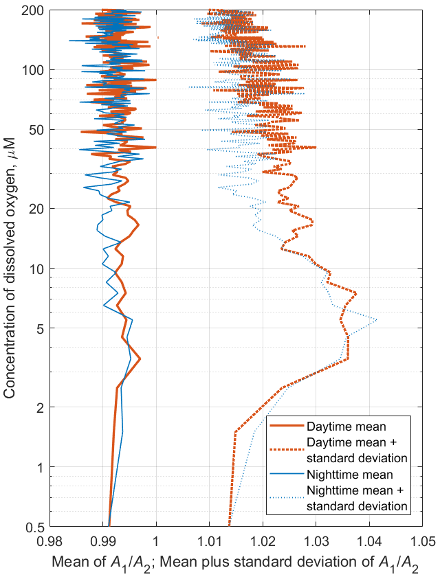
Figure A1Monthly averages of the depth profiles of the acoustic backscattering amplitude ratio for the time series of the daytime (solid red line) and nighttime (blue solid line) data in July 2019. Dotted lines indicate the values of the standard deviations from the means.
Underlying research data can be accessed via https://doi.org/10.13140/RG.2.2.28470.73285 (Ostrovskii et al., 2020) and https://doi.org/10.13140/RG.2.2.27548.62084 (Solovyev et al., 2021).
AGO analyzed the moored profiler Aqualog data and wrote the parts of the paper related to the profiler mooring measurements and data analysis. EGA analyzed the net zooplankton data and wrote the parts of the paper related to the zooplankton distribution analysis. VAS deployed the mooring and handled the profiler sensors. DAS is a design engineer of the profiler, who also maintained the profiler.
The authors declare that they have no conflict of interest.
Publisher's note: Copernicus Publications remains neutral with regard to jurisdictional claims in published maps and institutional affiliations.
We thank Andrey Zatsepin for promoting the moored profiler measurement program in the Black Sea. The Black Sea field study is carried out in the framework of Russian Ministry of Science and High Education, assignment no. 0128-2021-0016. The net sampling data analysis is supported by the Russian Science Foundation, grant no. 20-17-00167. The Aqualog profiler data processing and analysis are supported via grant nos. 19-05-00459 and 19-45-230012 by the Russian Fund for Basic Research and Krasnodarsky Kray Ministry of Science, Education, and Youth Policy. We are grateful to the editor and three anonymous referees for helpful comments on this paper.
This research has been supported by the Ministry of Science and Higher Education of the Russian Federation (grant no. 0128-2021-0016) and the Russian Foundation for Basic Research (grant nos. 19-05-00459 and 19-45-230012).
This paper was edited by Mario Hoppema and reviewed by four anonymous referees.
Alldredge, A. L., Robison, B. H., Fleminger, A., Torres, J. J., King, J. M., and Hamner, W. M.: Direct sampling and in situ observation of a persistent copepod aggregation in the mesopelagic zone of the Santa Barbara Basin, Mar. Biol., 80, 75–81, 1984.
Andrusov, N. I.: Preliminary report on the Black Sea cruise, Izvestiya Imperatorskogo Russkogo Geographicheskogo Obschestva [Bulletin of the Imperial Russian Geographic Society], 26, 398–409, 1890 (in Russian).
Arashkevich, E., Svetlichny, L., Gubareva, E., Besiktepe, S., Gücü, A. C., and Kideys, A. E.: Physiological and ecological studies of Calanus euxinus (Hulsemann) from the Black Sea with comments on its life cycle, in: Ecosystem modelling as a management tool for the Black Sea, edited by: Ivanov L. I. and Oguz, N., Kluwer Academic Publishers, Dordrecht, 351–365, 1998.
Arashkevich, E., Ostrovskii, A., and Solovyev, V.: Observations of water column habitats by combining acoustic backscatter data and zooplankton sampling in the NE Black Sea, 40th CIESM Congress Proceedings, Marseille, France, 28 October–1 November 2013, 40, 722, available at: http://www.ciesm.org/online/archives/abstracts/pdf/40/index.php (last access: 19 July 2021), 2013.
Arashkevich, E. G., Stefanova, K., Bandelj, V., Siokou, I., Kurt, T. T., Örek, Y. A., Timofte, F., Timonin, A., and Solidoro, C.: Mesozooplankton in the open Black Sea: Regional and seasonal characteristics, J. Marine Syst., 135, 81–96, https://doi.org/10.1016/j.jmarsys.2013.07.011, 2014.
Arashkevich, E. G., Louppova, N. E., Nikishina, A. B., Pautova, L. A., Chasovnikov, V. K., Drits, A. V., Podymov, O. I., Romanova, N. D., Stanichnaya, R. R., Zatsepin, A. G., Kuklev, S. B., and Flint, M. V.: Marine environmental monitoring in the shelf zone of the Black Sea: Assessment of the current state of the pelagic ecosystem, Oceanology, 55, 871–876, https://doi.org/10.1134/S0001437015060016, 2015.
Ashjian, C. J., Smith, S. L., Flagg, C. N., and Wilson, C.: Patterns and occurrence of diel vertical migration of zooplankton biomass in the Mid-Atlantic Bight described by an acoustic Doppler current profiler, Cont. Shelf Res., 18, 831–858, 1998.
Baumgartner, M. F. and Tarrant, A. M.: the physiology and ecology of diapause in marine copepods, Annu. Rev. Mar. Sci., 9, 387–411, https://doi.org/10.1146/annurev-marine-010816-060505, 2017.
Benfield, M. C., Davis, C. S., and Gallager, S. M.: Estimating the in situ orientation of Calanus finmarchicus on Georges Bank using the Video Plankton Recorder, Plankton Biol. Ecol., 47, 69–72, 2000.
Besiktepe, S.: Diel vertical distribution, and herbivory of copepods in the south-western part of the Black Sea, J. Marine Syst., 28, 281–301, https://doi.org/10.1016/S0924-7963(01)00029-X, 2001.
Bianchi, D., Galbraith, E., Carozza, D., Mislan, K. A. S., and Stock, C. A.: Intensification of open-ocean oxygen depletion by vertically migrating animals, Nat. Geosci., 6, 545–548, https://doi.org/10.1038/ngeo1837, 2013.
Campbell, R. W. and Dower J. F.: Role of lipids in the maintenance of neutral buoyancy by zooplankton, Mar. Ecol. Prog. Ser., 263, 93–99, https://doi.org/10.3354/meps263093, 2003.
Codispoti, L. A., Friederich, G. E., Murray, J. W., and Sakamoto, C. M.: Chemical variability in the Black Sea: implications of continuous vertical profiles that penetrated the oxic/anoxic interface, Deep-Sea Res. Pt. I, 38, Suppl. 2, S691–S710, 1991.
Drits, A. V. and Utkina, S. V.: Sagitta setosa feeding in the deep layers of high plankton concentration during daytime in the Black Sea, Oceanology, 28, 1014–1018, 1988.
Erkan, F. and Gücü, A. C.: Analyzing shipborne ADCP measurements to estimate distribution of southern Black Sea zoo plankton, Proceedings of the 4th European Conference on Underwater Acoustics, Rome, 1, 267–274, 1998.
Flagg, C. N. and Smith, S. L.: On the use of the acoustic Doppler current profiler to measure zooplankton abundance, Deep-Sea Res., 36, 455–474, 1989.
Flint, M. V.: Vertical distribution of mass zooplankton species in lower layers of aerobic zone in relation to the structure of oxygen field, in: Structure and production characteristics of planktonic populations in the Black Sea, edited by: Vinogradov, M. E. and Flint, M. V., Nauka, Moscow, 187–213, 1989 (in Russian).
Flint, M. V., Drits, A. V., and Pasternak, A. F.: Characteristic features of body composition and metabolism in some in some interzonal copepods, Mar. Biol., 111, 199–205, 1991.
Glazer, B. T., Luther, G. W., Konovalov, S. K., Friederich, G. E., Trouwborst, R. E., and Romanov, A. S.: Spatial and temporal variability of the Black Sea suboxic zone, Deep-Sea Res. Pt. II, 53, 1756–1768, https://doi.org/10.1016/j.dsr2.2006.03.022, 2006.
Heywood, K. J., Scrope-Howe, S., and Barton, E. D.: Estimation of zooplankton abundance from shipborne ADCP backscatter, Deep-Sea Res., 38, 667–691, 1991.
Hirche, H., Barz, K., Ayon, P., and Schulz, J.: High resolution vertical distribution of the copepod Calanus chilensis in relation to the shallow oxygen minimum zone off northern Peru using LOKI, a new plankton imaging system, Deep-Sea Res. Pt I, 88, 63–73, https://doi.org/10.1016/j.dsr.2014.03.001, 2014.
Hofmann, H. and Peeters, F.: In-Situ optical and acoustical measurements of the buoyant cyanobacterium P. Rubescens: Spatial and temporal distribution patterns, PLoS ONE, 8, e80913, https://doi.org/10.1371/journal.pone.0080913, 2013.
Kiørboe, T., Andersen, A., Langlois, V. J., Jakobsen, H. H., and Bohr, T.: Mechanisms and feasibility of prey capture in ambush-feeding zooplankton, P. Natl. Acad. Sci. USA, 106, 12394–12399, https://doi.org/10.1073/pnas.0903350106, 2009.
Klyuvitkin, A. A., Ostrovskii, A. G., Novigatskii, A. N., and Lisitzin, A. P.: Multidisciplinary experiment on studying short-period variability of the sedimentary process in the northeastern part of the Black Sea, Dokl. Earth Sci., 469, 771–775, https://doi.org/10.1134/S1028334X16070230, 2016.
Konovalov, S. K., Murray, J. W., and Luther, G. W.: Basic processes of Black Sea biogeochemistry, Oceanography, 18, 24–35, https://doi.org/10.5670/oceanog.2005.39, 2005.
Lavery, A. C., Wiebe, P. H., Stanton, T. K., Lawson, G. L., Benfield, M. C., and Copley, N.: Determining dominant scatterers of sound in mixed zooplankton populations, J. Acoust. Soc. Am., 122, 3304–3326, https://doi.org/10.1121/1.2793613, 2007.
Lawson, G. L., Wiebe, P. H., Ashjian, C. J., Chu, D., and Stanton, T. K.: Improved parameterization of Antarctic krill target strength models, J. Acoust. Soc. Am., 119, 232–242, https://doi.org/10.1121/1.2141229, 2006.
Morozov, A., Kuzenkov, O. A., and Arashkevich, E. G.: Modelling optimal behavioural strategies in structured populations using a novel theoretical framework, Sci. Rep.-UK, 9, 15020, https://doi.org/10.1038/s41598-019-51310-w, 2019.
Murray, J. W., Jannash, H. W., Honjo, S., Anderson, R. F., Reeburgh, W. S., Top, Z., Friederich, G.,E., Codispoti, L.,A., and Izdar, E.: Unexpected changes in the oxic/anoxic interface in the Black Sea, Nature, 338, 411–413, 1989.
Mutlu, E.: Acoustical identification of the concentration layer of a copepod species, Calanus euxinus, Mar. Biol., 142, 517–523, https://doi.org/10.1007/s00227-002-0986-3, 2003.
Mutlu, E.: Diel vertical migration of Sagitta setosa as inferred acoustically in the Black Sea, Mar. Biol., 149, 573–584, https://doi.org/10.1007/s00227-005-0221-0, 2006.
Mutlu, E.: Compared studies on recognition of marine underwater biological scattering layers, J. Appl. Biol. Sci., 1, 113–119, 2007.
Nikitin, V. N.: La distribution verticale du plancton dans la mer Noire. I. Copepoda et Cladocera, Trudy Osoboi Zoologicheskoi Laboratorii i Sevastopol'skoi Biologicheskoi Stantsii, Ser. 2, No. 5–10, 93–140, 1926 (in Russian; abstract in French).
Oguz, T., Tugrul, S., Kideys, A. E., Ediger, V., and Kubilay, N.: Physical and biogeochemical characteristics of the Black Sea, in: The Sea, Volume 14B: The Global Coastal Ocean Interdisciplinary Regional Studies and Syntheses, edited by: Robinson, A. R. and Brink, K. H., Harvard University Press, Cambridge, MA, 1331–1369, ISBN 9780674021174, 2006.
Ostrovskii, A. G. and Zatsepin, A. G.: Short-term hydrophysical and biological variability over the northeastern Black Sea continental slope as inferred from multiparametric tethered profiler surveys, Ocean Dynam., 61, 797–806, https://doi.org/10.1007/s10236-011-0400-0, 2011.
Ostrovskii, A. G. and Zatsepin, A. G.: Intense ventilation of the Black Sea pycnocline due to vertical turbulent exchange in the Rim Current area, Deep-Sea Res. Pt. I, 116, 1–13, https://doi.org/10.1016/j.dsr.2016.07.011, 2016.
Ostrovskii, A. G., Zatsepin, A. G., Soloviev, V. A., Tsibulsky, A. L., and Shvoev, D. A.: Autonomous system for vertical profiling of the marine environment at a moored station, Oceanology, 53, 233–242, https://doi.org/10.1134/S0001437013020124, 2013.
Ostrovskii, A. G., Zatsepin, A. G., Solovyev, V. A., and Soloviev, D. M.: The short timescale variability of the oxygen inventory in the NE Black Sea slope water, Ocean Sci., 14, 1567–1579, https://doi.org/10.5194/os-14-1567-2018, 2018.
Ostrovskii, A. G., Solovyev, V. A., and Shvoev, D. A.: Inventory of the Moored Profiler Aqualog Data on the Directional Acoustic Backscatter Ratio in the Lower Part of the Oxycline and Hypoxic Zone in the NE Black Sea Slope Water from 2013–2020, https://doi.org/10.13140/RG.2.2.28470.73285, ResearchGate [data set], 2020.
Petipa, T. S., Sazhina, L. I., and Delalo, E. P.: Vertical distribution of zooplankton in the Black Sea in relation to the hydrological conditions, Dokl. Akad. Nauk SSSR+, 133, 964–967, 1960 (in Russian).
Pezacki, P. D., Gorska, N., and Soloviev, V.: An acoustic study of zooplankton diel vertical migration in the Black Sea, Hydroacoustics, 20, 139–148, 2017.
Roberts, P. L. D. and Jaffe, J. S.: Multiple angle acoustic classification of zooplankton, J. Acoust. Soc. Am., 121, 2060–2070, https://doi.org/10.1121/1.2697471, 2007.
Roberts, P. L. D. and Jaffe, J. S.: Classification of live, untethered zooplankton from observations of multiple-angle acoustic scatter, J. Acoust. Soc. Am., 124, 796–802. https://doi.org/10.1121/1.2945114, 2008.
Sakınan, S. and Gücü, A. C.: Spatial distribution of the Black Sea copepod, Calanus euxinus, estimated using multi-frequency acoustic backscatter, ICES J. Mar. Sci., 74, 832–846, https://doi.org/10.1093/icesjms/fsw183, 2016.
Sartoris, F. J., Thomas, D. N., Cornils, A., and Schnack-Schiel, S. B.: Buoyancy and diapause in Antarctic copepods: the role of ammonium accumulation, Limnol. Oceanogr., 55, 1860–1864, https://doi.org/10.4319/lo.2010.55.5.1860, 2010.
Schründer, S., Schnack-Schiel, S. B., Auel, H., and Sartoris, F. J.: Control of diapause by acidic pH and ammonium accumulation in the haemolymph of Antarctic copepods, PLOS ONE, 8, e77498, https://doi.org/10.1371/journal.pone.0077498, 2013.
Smeti, H., Pagano, M., Menkes, C., Boissieu, F., Lebourges-Dhaussy, A., Hunt, B. P. V., Allain, V., Rodier, M., Kestenare, E., and Sammari, C.: Spatial and temporal variability of zooplankton off New Caledonia (Southwestern Pacific) from acoustics and net measurements, J. Geophys. Res.-Oceans, 120, 2676–2700, https://doi.org/10.1002/2014JC010441, 2015.
Solovyev, V. A., Shvoev, D. A., and Ostrovskii, A. G.: Metadata of Aqualog profiler sreveys in 2013–2021, https://doi.org/10.13140/RG.2.2.27548.62084, ResearchGate [data set], 2021.
Stanton, T. K. and Chu, D.: Review and recommendations for the modelling of acoustic scattering by fluid-like elongated zooplankton: euphausiids and copepods, ICES J. Mar. Sci., 57, 793–807, https://doi.org/10.1006/jmsc.1999.0517, 2000.
Stanton, T. K., Chu, D., Wiebe, P. H., and Clay, C. S.: Average echoes from randomly oriented random-length finite cylinders: Zooplankton models, J. Acoust. Soc. Am., 94, 3463–3472, https://doi.org/10.1121/1.407200, 1993.
Stanton, T. K., Wiebe, P. H., Chu, D., Benfield, M., Scanlon, L., Martin, L., and Eastwood, R. L.: On acoustic estimates of zooplankton biomass, ICES J. Mar. Sci., 51, 505–512. 1994.
Stefanova, K. and Marinova, V.: Zooplankton distribution and sound scattering layers in the Bulgarian Black Sea area – A case study Cape Galata Transect, Intl. J. Appl. Eng. Res., 10, 35998–36003, 2015.
Svetlichny, L. S., Hubareva, E. S., and Arashkevich, E. G.: Physiological and behavioural response to hypoxia in active and diapausing stage V copepodites of Calanus euxinus, in: Arch. Hydrobiol. Spec. Issues, Advanc. Limnol., Evolutionary and ecological aspects of crustacean diapause, edited by: Brendonck, L., de Meester, L., and Hairston, Schwelzerbart'sche Verlagsbuchhandlung, Stuttgart, 52, 507–519, 1998.
Svetlichny, L. S., Hubareva, E. S., Erkan, F., and Gucu, A. C.: Physiological and behavioral aspects of Calanus euxinus females (Copepoda: Calanoida) during vertical migration across temperature and oxygen gradients, Mar. Biol., 137, 963–971, 2000.
Svetlichny, L., Gubareva, E., and Arashkevich, E.: Effect of oxygen concentration on energy metabolism in the migrating and diapausing copepods Calanus euxinus in the Black Sea, Oceanology, 42, 670–676, 2002.
Svetlichny, L. S., Kideys, A. E., Hubareva, E. S., Besiktepe, S., and Isinibilir, M.: Development and lipid storage in Calanus euxinus from the Black and Marmara seas: variabilities due to habitat conditions, J. Marine Syst., 59, 52–62, https://doi.org/10.1016/j.jmarsys.2005.09.003, 2006.
Svetlichny, L. S., Yuneva, T. V., Hubareva, E. S., Schepkina, A. M., Besiktepe, S., Kideys, A. E., Bat, L., and Sahin F.: Development of Calanus euxinus during spring cold homothermy in the Black Sea, Mar. Ecol. Prog. Ser., 374, 199–213, https://doi.org/10.3354/meps07740, 2009.
Tutasi, P. and Escribano, R.: Zooplankton diel vertical migration and downward C flux into the oxygen minimum zone in the highly productive upwelling region off northern Chile, Biogeosciences, 17, 455–473, https://doi.org/10.5194/bg-17-455-2020, 2020.
Vinogradov, M. E. and Nalbandov, Y. R.: Influence of water density on the distribution of physical, chemical, and biological characteristics of the Black Sea pelagic ecosystem, Oceanology, 30, 769–777, 1990.
Vinogradov, M. E., Flint, M. V., and Shushkina, E. A.: Vertical distribution of mesozooplankton in the open Black Sea, Mar. Biol., 89, 95–107, 1985.
Vinogradov, M. E., Arashkevich, E. G., and Ilchenko, S. V.: The ecology of the Calanus ponticus population in the deeper layer of its concentration in the Black Sea, J. Plankton Res., 14, 447–458, 1992.
Visser, A. W. and Jónasdóttir S. H.: Lipids, buoyancy, and the seasonal vertical migration of Calanus finmarchicus, Fish. Oceanogr., 8, 100–106, 1999.
Wiebe, P. H., Stanton, T. K., Greene, C. H., Benfield, M. C., Sosik, H. M., Austin, T. C., Warren, J. D., and Hammar, T.: BIOMAPER-II: an integrated instrument platform for coupled biological and physical measurements in coastal and oceanic regimes, IEEE J. Oceanic Eng., 27, 700–716, 2002, https://doi.org/10.1109/JOE.2002.1040951, 2002.
Wishner, K. F., Seibel, B., and Outram, D.: Ocean deoxygenation and copepods: coping with oxygen minimum zone variability, Biogeosciences, 17, 2315–2339, https://doi.org/10.5194/bg-17-2315-2020, 2020.
Yakushev, E. V., Podymov, O. I., and Chasovnikov, V. K.: Seasonal changes in the hydrochemical structure of the Black Sea redox zone, Oceanography, 18, 48–55, https://doi.org/10.5670/oceanog.2005.41, 2005.
Yunev, O. A., Carstensen, J., Stelmakh, L. V., Belokopytov, V. N., and Suslin, V. V.: Reconsideration of the phytoplankton seasonality in the open Black Sea, Limnol. Oceanogr. Lett., 6, 51–59, https://doi.org/10.1002/lol2.10178, 2020.