Coastal submesoscale processes and their effect on phytoplankton distribution in the southeastern Bay of Biscay

Submesoscale processes have a determinant role in the dynamics of oceans by transporting momentum, heat, mass, and particles. Furthermore, they can define niches where different phytoplankton species flourish and accumulate not only by nutrient provisioning but also by modifying the water column structure or active gathering through advection. In coastal areas, however, submesoscale oceanic processes act together with coastal ones, and their effect on phytoplankton distribution is not straightforward. The present study brings the relevance of hydrodynamic variables, such as vorticity, into consideration in the study of phytoplankton distribution, via the analysis of in situ and remote multidisciplinary data. In situ data were obtained during the ETOILE oceanographic cruise, which surveyed the Capbreton Canyon area in the southeastern part of the Bay of Biscay in early August 2017. The main objective of this cruise was to describe the link between the occurrence and distribution of phytoplankton spectral groups and mesoscale to submesoscale ocean processes. In situ discrete hydrographic measurements and multi-spectral chlorophyll a (chl a) fluorescence profiles were obtained in selected stations, while temperature, conductivity, and in vivo chl a fluorescence were also continuously recorded at the surface. On top of these data, remote sensing data available for this area, such as high-frequency radar and satellite data, were also processed and analysed. From the joint analysis of these observations, we discuss the relative importance and effects of several environmental factors on phytoplankton spectral group distribution above and below the pycnocline and at the deep chlorophyll maximum (DCM) by performing a set of generalized additive models (GAMs). Overall, salinity is the most important parameter modulating not only total chl a but also the contribution of the two dominant spectral groups of phytoplankton, brown and green algae groups. However, at the DCM, among the measured variables, vorticity is the main modulating environmental factor for phytoplankton distribution and explains 19.30 % of the variance. Since the observed distribution of chl a within the DCM cannot be statistically explained without the vorticity, this research sheds light on the impact of the dynamic variables in the distribution of spectral groups at high spatial resolution.

1 Introduction

The monitoring and characterization of submesoscale dynamics are determinant for the appropriate comprehension of marine ecosystems (Lévy et al., 2012). Submesoscale processes refer to those features that range on spatio-temporal scales of the order of 0.1–10 km and 0.1–10 d. The timescales at which these processes evolve make them uniquely important to the structure and functioning of planktonic ecosystems (Lévy et al., 2012; Mahadevan, 2016). They influence the ecosystem by either driving episodic nutrient pulses to the sunlit surface, affecting the mean time that photosynthetic organisms remain in the well-lit surface (Lévy et al., 2012), or reducing and even suppressing the biological production (Gruber et al., 2011). In addition, since primary production drives the absorption of atmospheric CO₂, submesoscale processes might actively contribute to the carbon export and regulate the fate of particulate organic carbon (Mahadevan, 2014). The effect of submesoscale processes on phytoplankton also has implications for regional biogeochemical budgets, plankton monitoring strategies, fisheries, and management (Irigoien et al., 2007).

The influence of ocean dynamics on phytoplankton covers a wide range of spatio-temporal scales, and these are inherent to the surveying strategy being selected. D'Ovidio et al. (2010) linked the occurrence of different phytoplankton groups with the large-scale surface ocean dynamics based on altimetry data. They defined the so-called fluid dynamical niches where the phytoplankton assemblages occur within distinct physicochemical environments. However, available satellite observations lack the spatio-temporal resolution to properly resolve the fast-evolving submesoscale coastal processes. In coastal regions, where oceanic currents meet the sea floor, the connection between the submesoscale processes and phytoplankton becomes even more challenging and therefore requires more demanding surveying methods that can provide a high spatio-temporal resolution. Nowadays, autonomous gliders can typically cover 1 km horizontally in an hour, but even this can be too slow for synoptic measurements of larger submesoscale features (on scales of 10 km). An alternative is the use of ship-towed undulating devices, which allow sampling 10–20 times faster than a glider (Lévy et al., 2012). Regarding phytoplankton distribution, submesoscale to microscale vertical patterns of chlorophyll a (chl a) concentrations have been studied widely by the use of in vivo fluorometric casts, allowing the identification of the deep chlorophyll maximum (DCM) (Cullen, 2015). Differences within the DCM in terms of concentration, biomass, and diversity stress the importance of the environmental drivers involved (Latasa et al., 2017), upon which the occurrence of (sub)mesoscale processes play a critical role (Lévy et al., 2012).

This study focuses on the innermost southeastern region of the Bay of Biscay (SE-BoB), a semi-open bay delimited by the Spanish coast in the south and the French coast in the east. The BoB is an area of complex coastal hydrographic and hydrodynamic processes, mainly due to the intricate bathymetry, the seasonally modulated and episodically strong river runoff, the wind- and density-driven ocean circulation, and their interplay. The circulation in the coastal SE-BoB is controlled mainly by the prevailing winds, although the general pattern is characterized by a weak anticyclonic circulation in the central deeper region (Valencia et al., 2004; Pingree and Garcia-Soto, 2014). The wind pattern either reinforces or weakens the seasonal Iberian Poleward Current (IPC), which flows cyclonically over the slope in autumn and winter (Rubio et al., 2013). The IPC is, due to the effect of bathymetry, responsible for the generation of Slope Water Oceanic eDDIES (SWODDIES) (Caballero et al., 2016; Teles-Machado et al., 2016). Besides, the ocean surface layer in this region is subjected to the seasonal variations of the water runoff from the main nearby rivers: the Gironde, Loire, and Adour rivers (Reverdin et al., 2013). The river runoff significantly modifies the water mass adjacent to the shelf by creating turbid and diluted plumes (Ferrer et al., 2009), which act as a nutrient source to the surface layers and sustain primary production in the region (Morozov et al., 2013).

These complex ocean dynamics can modulate phytoplankton occurrence in the BoB. The flow of the IPC generates a shelf-break convergent front that separates the advected high-salinity and warm waters from the cold fresher coastal waters. The vertical mixing associated with this frontal system has a substantial influence on the whole plankton community (Fernández et al., 1993). Caballero et al. (2016) reported a DCM in the centre of a SWODDY resulting from the vertical velocities and eddy-wind-induced Ekman pumping in the centre of the anticyclone. More recently, Muñiz et al. (2019) described the phytoplankton annual cycle in the SE-BoB and reported that temperature and nutrients explained most of the of the variability of chl a concentration. Nevertheless, to our knowledge, none of these studies have focused on the relative importance of submesoscale dynamics while analysing hydrographic and hydrodynamic forcing mechanisms at the same time.

In order to shed light on the coastal submesoscale dynamics and their effects on chl a and phytoplankton groups distribution, the ETOILE oceanographic cruise surveyed the Capbreton Canyon area in early August 2017. This cruise was one of the research actions in the framework of the European H2020 Joint European Research Infrastructure for Coastal Observatory – Novel European eXpertise for coastal observaTories (JERICO-NEXT) project. The regional coastal observatories (EuskOOS) are also embedded in the JERICO Research Infrastructure and provide the operational high-frequency (HF) radar data complementing the ETOILE in situ measurements. JERICO-NEXT (2014–2019), its predecessor JERICO (2007–2013), and the ongoing JERICO-S3 (2020–2024) all aim to consolidate a pan-European coastal observatory infrastructure for a better understanding of the functioning of coastal marine systems and a better assessment of their changes. In this study, we first describe the submesoscale processes that are present in the study area based on the joint analysis of a wide range of multiplatform spatio-temporal data, from remote sensing to in situ measurements. Secondly, we investigate the link between the observed submesoscale structures and the distribution of the two dominant spectral groups of phytoplankton, estimated with multi-spectral chl a fluorescence technique above and below the pycnocline and at the DCM, by performing a set of general additive models (GAMs).

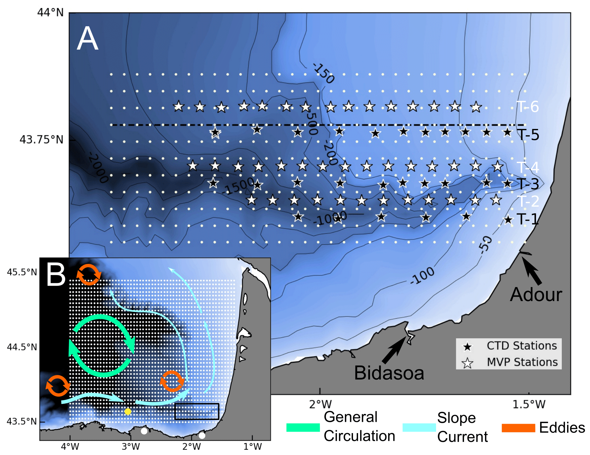
Figure 1 Sampling map and circulation in the Bay of Biscay. Location of the conductivity–temperature–depth (CTD) and moving vessel profiler (MVP) stations (a). At uneven transects (T-1, T-3, and T-5), black stars mark the CTD stations where vertical casts of temperature, salinity, and in vivo multi-spectral chlorophyll a (chl a) fluorescence were collected. At even transects, white stars mark the location of the point at which MVP data have been averaged, located every 5 km. White dots represent the grid at which these measurements were interpolated, and the dashed black line marks the cross section at 43.77^∘ N analysed in Figs. 5 and 7. The locations of the Adour and Bidasoa rivers are shown by the black arrows. Seasonal to mesoscale circulation in the Bay of Biscay (b). The small white dots represent the HF radar grid, the yellow dot corresponds to the location of the oceano-meteorological buoy used for the wind data, and large white dots mark the location of the HF radar antennas. The black rectangle shows the area covered by the in situ sampling during ETOILE survey, which is zoomed in (a).

2 Material and methods

2.1 In situ data from the ETOILE cruise

In the framework of the European H2020 JERICO-NEXT project, RV Côtes de la Manche (CNRS-INSU), surveyed the area of Capbreton Canyon from 2 to 4 August 2017 during Leg 2.2 of the ETOILE oceanographic cruise (P.I. Pascal Lazure, IFREMER, https://campagnes.flotteoceanographique.fr/campagnes/17010800/, last access: 11 June 2021), aiming to unravel the mesoscale and submesoscale dynamics in the area. The cruise consisted of six transects covering the continental shelf and slope, as well as the axis of the canyon, as shown in Fig. 1. During east–west transects (T1, T3, and T5), a CTD (Sea-Bird) was deployed every ∼ 7 km, while during west–east transects (T2, T4, and T6) a moving vessel profiler (MVP200 operated by Genavir) was towed, and the profiles were averaged every 5 km. As a good compromise in terms of spatial resolution and coverage of the observations was important, the use of the moving vessel profiler (MVP) allowed a more extensive and quicker sampling suitable for small, rapidly evolving structures.

During the cruise, chl a was estimated by a FluoroProbe (bbe Moldakenke) multi-spectral fluorometer, which measured chl a and accessory pigments using light-emitting diodes (LEDs) with different wavebands. Therefore, it was possible to distinguish between four algal pigmentary groups: “blue algae” (e.g. phycocyanin-containing Cyanobacteria), “Green algae” (e.g. Chrolorophytes, Chrysophytes), “brown algae” (e.g. Diatoms, Dinoflagellates) and a “mixed red group” (e.g. phycoerythrin-containing Cyanobacteria, Cryptophytes). The FluoroProbe estimated chl a equivalent (ChlaEQL-1) concentrations for these four groups and total chl a following the algorithms of Beutler et al. (2002), as explained in MacIntyre et al. (2010), and using the manufacturer's calibration, and they also provided an estimation of the concentration of chromophoric dissolved organic matter (CDOM or yellow substances). In vivo chl a profiles were obtained up to 80 m depth. Unfortunately, this data could only be gathered in the T3 and T5 transects due to connection issues with the instrument during T1. During the whole cruise, salinity and in vivo chl a were continuously measured on the surface (3.5 m deep) by a thermosalinograph and a second automated FluoroProbe multi-spectral fluorometer, respectively.

2.2 Complementary operational remote sensing data

In addition to the in situ data, remote sensing operational data were used to complete the picture obtained during ETOILE. Ocean surface current measurements were obtained by two long-range high-frequency (HF) radar antenna located at Cape Matxitxako and Cape Higer. The antennas are owned by the Directorate of Emergency Attention and Meteorology of the Basque Security Department and are part of EuskOOS network (https://www.euskoos.eus/en/, last access: 11 June 2021). They emit at a central frequency of 4.463 MHz and a 30 kHz bandwidth and provide hourly horizontal currents maps (corresponding to vertically integrated horizontal velocities in the first 3 m of the water column) (Rubio et al., 2013). The receiving signal, an averaged Doppler backscatter spectrum, allows for the estimation of surface currents over wide areas (reaching distances over 100 km from the coast) with high spatial (1–5 km) and temporal (≤ 1 h) resolution (Fig. 1b). To obtain the surface velocity data, we followed the methodology detailed in Rubio et al. (2013). Velocity data is processed from the spectra of the received echoes every 20 min using the MUSIC (MUltiple SIgnal Classification) algorithm. Following this, a centred 3 h running average was applied to the resulting radial velocity fields as part of the pre-processing previous to the computation of total currents. The current velocity data were quality-controlled using procedures based on velocity and variance thresholds, signal-to-noise ratios, and radial total coverage, following standard recommendations (Mantovani et al., 2020). The performance of this system and its potential for the study of ocean processes and transport patterns have already been demonstrated by previous works (e.g. Rubio et al., 2011, 2018; Solabarrieta et al., 2014; Caballero et al., 2020).

In order to visualize representative velocity fields, we applied a 10th-order digital Butterworth low-pass filter (Emery and Thomson, 2001) to both velocity components at each node (filtering out T<48 h). Therefore, HF processes such as inertial currents or tides were removed, as these are irrelevant for this study and would have eclipsed the geostrophic and wind-induced current mesoscale and submesoscale patterns. A Lagrangian particle-tracking model (LPTM) was applied to HF radar data to simulate trajectories and analyse surface ocean transport patterns around the dates of the ETOILE survey. Particles released within the HF radar coverage area were advected using a 4th-order Runge–Kutta scheme (Benson, 1992). In this case, the particles are advected using the 2D hourly current fields given by the HF radar from 26 July to 11 August. To describe (sub)mesoscale patterns, Lagrangian residual currents (LRC) were calculated following a methodology similar to that described in Muller et al. (2009) using an integration time of 3 d.

Furthermore, satellite data prior to and after the cruise were also analysed. Sea surface temperature (SST) and satellite chl a data (chl-a^sat) were retrieved from the Visible and Infrared Imager/Radiometer Suite (VIIRS) sensor, and water turbidity was retrieved from MODIS. In addition to these datasets, hourly wind information of July and August was collected by the mooring buoy of Bilbao owned by Puertos del Estado (available in http://www.puertos.es/en-us, last access: 11 June 2021). Although its location is not exactly in our study area (Fig. 1b), it is considered close enough for a general description of the wind regime in the bay.

2.3 Computation of vorticity and vertical velocities

From hydrographic data alone, geostrophic circulation can be diagnosed, inferring various key dynamical variables, such as geostrophic relative vorticity (hereinafter referred to just as vorticity) or the vertical velocity from a 3D snapshot of the density field. To compute vertical velocities, we assume quasi-geostrophic dynamics and a synoptic or steady state, where the Rossby number is small ($Ro=U/fL\ll \mathrm{1}$, where U is the characteristic velocity, L is length scale, and f is the Coriolis parameter) and submesoscale features remain constant during the sampling (Gomis et al., 2001). To reduce the computational effort during the analysis of the data, the MVP transects were averaged every 5 km, considering it to be a high enough resolution for resolving submesoscale structures, following the methodology in Gomis et al. (2001). An interpolation of the data allows for deriving key dynamical variables, such as the geostrophic relative vorticity and vertical velocities. This was accomplished by merging the CTD and averaged MVP profiles after verifying that no significant bias was present between the measurements of these two instruments. Once having verified that data can be merged, the optimal statistical interpolation (OSI) was performed by the “DAToBJETIVO” software package developed by Gomis and Ruiz (2003) for the objective spatial analysis and the diagnosis of oceanographic variables.

For the interpolation in the sampling area, an 11×33 output grid was used with a $\mathrm{0.031}{}^{\circ }\times \mathrm{0.033}{}^{\circ }$ resolution (Fig. 1a), pursuing a compromise between providing a good representation of the scales that can be resolved by the sampling and minimizing the effect of the observational error. A Gaussian function for the correlation model between observations (assuming 2D isotropy) was set up, with a correlation length scale of 15 km. The noise-to-signal (NTS) variance ratio used for the analysis of temperature, salinity, and dynamic height was 0.01, 0.005, and 0.0027, respectively. This ratio was defined as the variance of the observational error divided by the variance of the interpolated field (the latter referring to the deviations between observations and the mean field). This parameter allows the inclusion in the analysis of an estimation of the observational error and adjustments of the weight of the observations on the analysis (the larger the NTS parameter, the smaller the influence of the observation). Following this, i.e. after the interpolation, all fields were spatially smoothed, with an additional low-pass filter with a cut-off length scale of 10 km to avoid aliasing errors due to unresolved structures. This resulted in a coarse grid that allowed the appropriate representation of the subsequent spatial derivatives of the analysed field. In the vertical, 98 equally spaced levels were considered, from 4 to 200 m (every 2 m). To analyse and correlate the explanatory and the response variables, the same interpolation was performed for the chl a data.

2.4 Statistical analysis

The presence of a well-defined seasonal pycnocline and a DCM were used as criteria to define three dynamically different layers in the water column, which have been analysed separately to constrain the different dynamical environments. Therefore, prior to the statistical analysis, the dataset was divided in three subsets: “above the pycnocline” (“APY”, containing data from 4 to 24 m depth), “below the pycnocline” (“BPY”, containing data from 26 to 74 m depth), and “at the DCM” (“DCM”, containing data from 26 to 74 m and where total chl-a≥1.5 µg ChlaEQL-1).

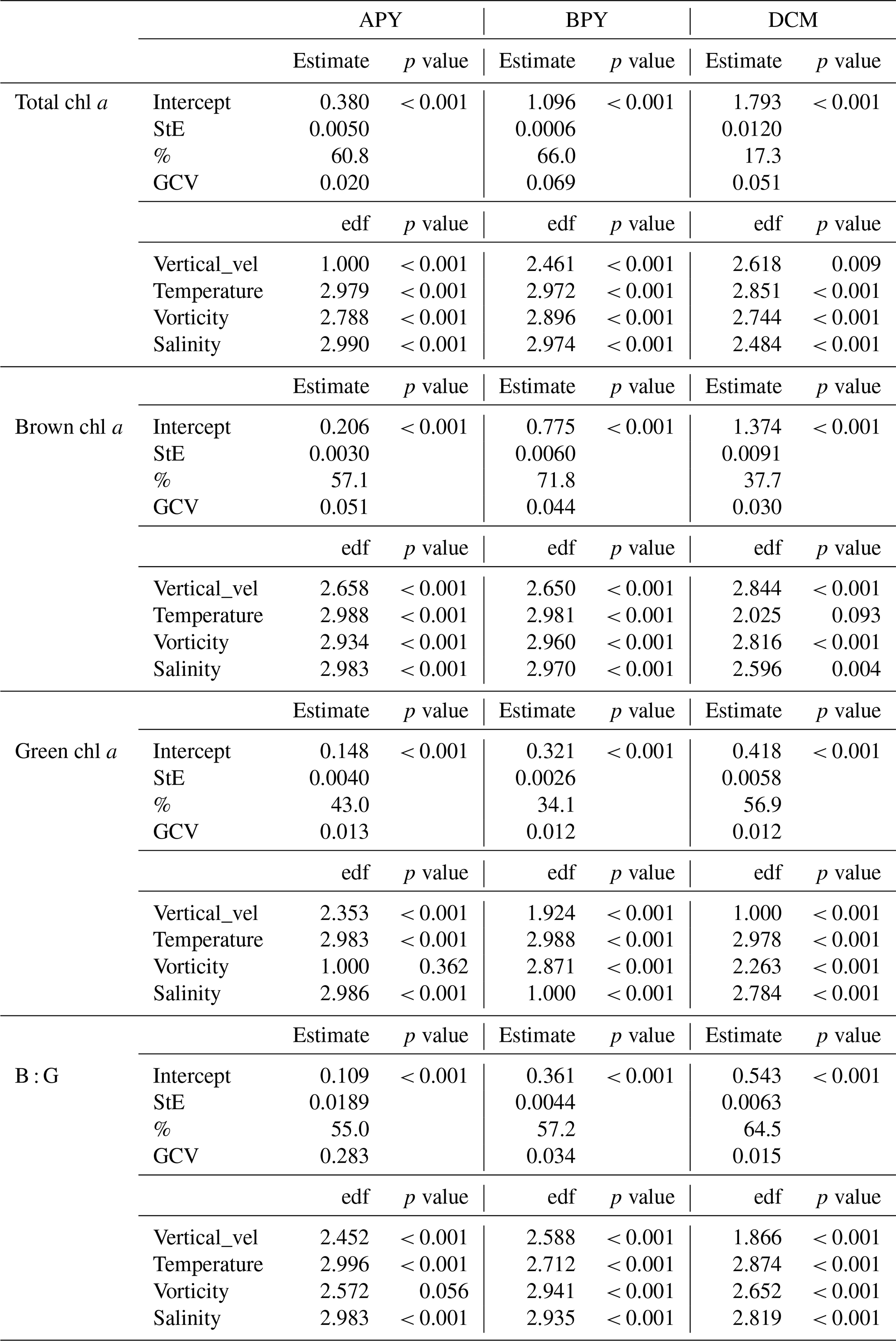
Table 1 Generalized additive model (GAM) results. Intercept, standard error (StE), significance (p value), and explained variance (%) of the GAMs for the water column sections “Above the pycnocline” (APY), “below the pycnocline” (BPY) and at the deep chlorophyll maximum (DCM). Dependent variables are the estimated chl a concentrations for the different algae groups, and B : G refers to the brown chl a to green chl a ratio. The estimated degrees of freedom (edf) and significance (p value) of the environmental variables are also included. Although salinity and temperature were correlated for the section BPY, both variables were kept since the fit (R² and general cross-validation, GCV) was better in all cases.

We assessed the relative importance of different environmental factors involved in the phytoplankton distribution by developing a statistical generalized additive model (GAM) (Hastie and Tibshirani, 1990). GAMs offer the possibility of identifying non-linear relationship between variables by the inclusion of a smoothing function that has no specific shape. Since the relationship among variables along the entire water column might mask each other, three GAMs were implemented for the different dynamical environments in the water column, as previously detailed, by using (Eq. 1):

$$\begin{array}{}\text{(1)}& \begin{array}{rl}& [\text{chl}-a{]}_z=a+g_{\mathrm{1}}[{\text{Sal}}_z]+g_{\mathrm{2}}[{\text{Temp}}_z]+g_{\mathrm{3}}[{\text{Vor}}_z]\\ & +g_{\mathrm{4}}\left[{\text{V.Vel}}_z\right]+\mathit{ϵ},\end{array}\end{array}$$

where (a) is an intercept, z is the location in the water column (APY, BPY, and DCM), g is the nonparametric smooth functions describing the effect of environment on chl a concentrations, and ϵ is an error term. Sal, Temp, Vor, and V. Vel correspond to the environmental variables determined in this study, salinity, temperature, vorticity (cyclonic or anticyclonic), and vertical velocities (upwelling or downwelling), respectively.

Figure 2 Wind direction and intensity at Bilbao's mooring buoy represented on a progressive vector diagram (PVD).

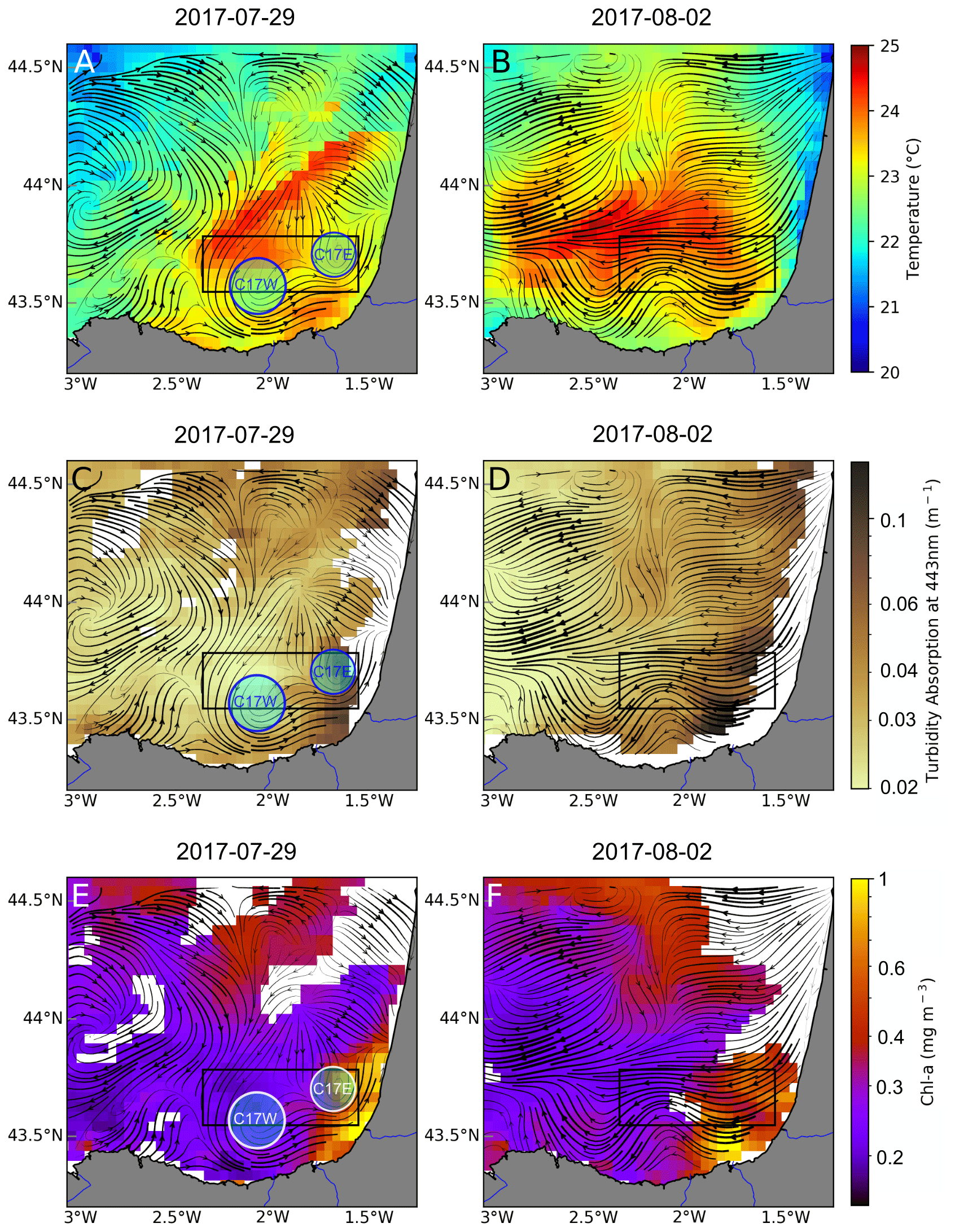
Figure 3 Satellite observations for SST (a, b), turbidity (c, d), and chl-a^sat (e, f) corresponding to 29 July (a, c, e) and 2 August (b, d, f). Black lines show the Lagrangian residual currents (LRC) calculated for the periods 26–29 July and 30 July to 2 August. The black box shows the study area, where ETOILE survey took place. The circles in the left column represent the approximate location of the observed cyclonic eddies (C17W and C17E). Turbidity and chl a are plotted on logarithmic scale.

In order to account for co-linearity problems, we calculated pairwise Spearman correlation coefficients (r) between variables. The only pair of variables correlated were salinity and temperature for the BPY subset ($r=-\mathrm{0.77}$, p value < 0.05) related to the depth dependency of both variables. The model selection was based on the analysis performed by Llope et al. (2009), where a stepwise approach was implemented by removing covariates and minimizing the generalized cross-validation (GCV) criterion of the model (Wood, 2000). The GCV criterion is a measure of the out-of-sample predictive performance of the model and is related to the Akaike information criterion (AIC) (Wood, 2006). Similarly, by deleting one variable at a time we can quantify the penalty on the explained variance of the phytoplankton distribution (Llope et al., 2009). In total, 12 GAMs were carried out from the combination of total chl a, green algae chl a (green chl a), brown algae chl a (brown chl a), and the brown chl a to green chl a ratio (B : G) among the three vertical subsets (Table 1). All the variables showed a significant impact on the total and group chl a distribution except the vorticity for the green chl a in the APY subset. If vorticity was removed, the model slightly improved (GCV decreased from 0.0130 to 0.0125; Table 2). However, we decided to keep it in the model for the different levels, keeping in mind that its impact in the APY subset was insignificant. In addition, vertical velocities for the APY subset show unrealistic values as an artefact of the surface boundary condition necessary to perform the calculations, where velocities are assumed to be null. Since the derived relationships with chl a are not considered realistic (even if they are included in the analysis and slightly improve the models), they are not considered further. The rest of the variables, even if they explained a small part of the variance, they significantly improved the model. The GAMs were carried out by using R (version 3.63, R Core Team, 2020) and the package mgcv (version 1.8.33) (Wood, 2011).

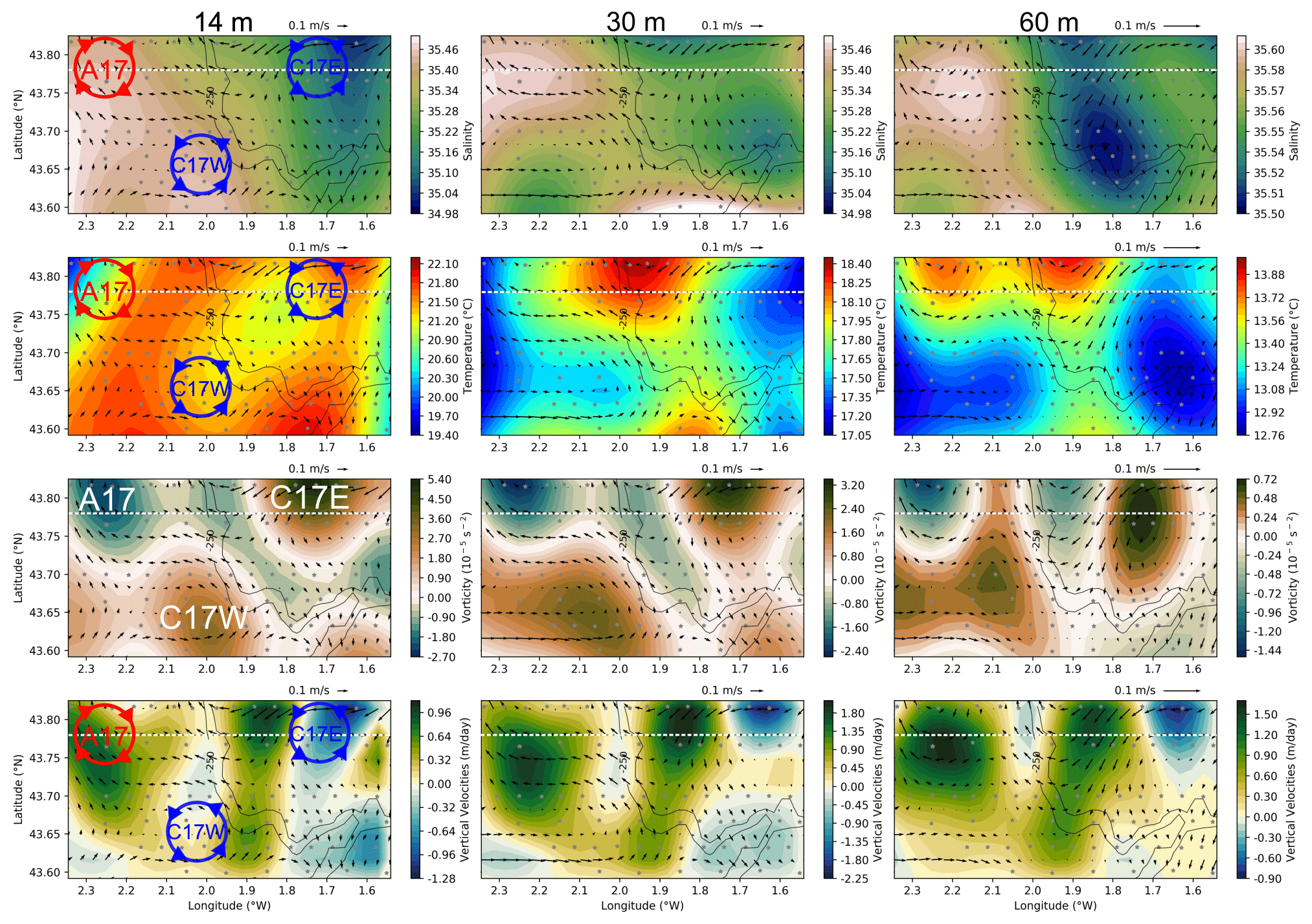
Figure 4 Synoptic plots for the hydrographic and hydrodynamical conditions for the period (2 to 4 August 2017). From top to bottom the following variables are shown: salinity, temperature, vorticity, and vertical velocity fields, at 14, 30, and 60 m (left to right). Black arrows correspond to the geostrophic velocities, and black contours represent the 200 and 250 m isobaths. The dashed white line corresponds to the cross section at 43.77^∘ N shown in Figs. 5 and 7. Negative vorticity values represents anticyclonic circulation, while positive values represent cyclonic circulation. Negative (positive) vertical velocity values represent downwelling (upwelling). The red (blue) circles drawn in the left column represent the approximate location of A17 (C17W and C17E). The scale range for each of the variables is different for each depth.

3 Results

3.1 Mapping coastal mesoscale hydrography and currents

The combined use of wind data and satellite imagery together with the HF radar provides a context of hydrographical and dynamical regime around the dates of the ETOILE cruise. Figure 2 shows the progressive vector diagram (PVD) of the wind conditions. From 21 to 28 July, the predominant wind has a marked northwesterly component with relatively high intensity. Afterwards, it decreases in intensity, shifts, and starts blowing from the northeast. On 7 August, the wind again has a northwest component for few days. Therefore, the wind conditions during the whole cruise remain almost constant in direction and low in intensity. Figure 3 shows the satellite SST, chl-a^sat, and turbidity fields; the latter allowed us to locate the river plumes of the Adour and the Bidasoa rivers. In addition, the LRC fields derived from the HF radar, which are superimposed onto the previous fields, give a high-resolution image of the surface transport during the days previous to the survey in the periods 26–29 July and 30 July to 2 August. The surface circulation patterns and position of the river plumes are observed to evolve from the first to the second periods. On 26–29 July (Fig. 3, left column), under northwesterly winds the circulation shows complex spatial patterns, and two cyclonic eddies, with diameters between 10–15 km, can be identified (C17W at 43.6^∘ N and 2^∘ W and C17E at 43.7^∘ N and 1.7^∘ W). During the period 30 July to 2 August (Fig. 3 – right column), the winds shift to northeasterly, which generates a remarkable transition to westward currents. At this moment, the cyclonic eddies are not visible to the HF radar. Instead, in their position, we observe a meandering pattern that affects the distribution of the SST and the position of the river plumes and their associated chl-a^sat signature. In addition, on 2 August, a sharp decrease in SST is observable close to the French inner shelf, which is linked with the upwelling generated by the northeasterly winds.

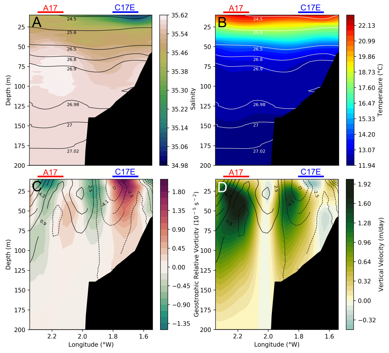
Figure 5 Cross section at 43.77^∘ N (location marked by dashed lines in Figs. 1 and 4), representing salinity (a) and temperature (b) with isopycnals (black and white contours, respectively) and vorticity (c) and vertical velocities (d) with meridional geostrophic velocities (solid (dashed) black contours for positive (negative) velocities) for the period (2 to 4 August 2017). Negative vorticity values represents anticyclonic circulation, while positive values represent cyclonic circulation. Positive (negative) values for geostrophic velocity represent a northward (southward) current. Negative (positive) vertical velocity values represent downwelling (upwelling). The red (blue) horizontal lines represent the horizontal extension of A17 (C17E) that the section crosses.

During the ETOILE cruise (2 to 4 August), the first metres of the water column are characterized by a high spatial variability (Fig. 4). Although the river plume is no longer visible in the salinity fields at 14 m, a layer of relatively fresh water is located in the inner continental shelf (1.6–1.7^∘ W). This low salinity front extends over 20 km horizontally and 18 m vertically (Fig. 5a) if we consider the isopycnal 35.1 as in Puillat et al. (2006). At 60 m depth (Fig. 4), a second salinity front is observed at the shelf break (i.e. along the 250 m isobath), with a vertical extension between 50 and 120 m (Fig. 5). Fresher waters, with salinities of ∼ 35.5 occupy the totality of the water column over the shelf, while oceanic waters at the slope are characterized by salinities over ∼ 35.6. The salinity range in the shelf break front is much smaller than in the surface front.

The cyclones depicted in Fig. 3 are also observed at deeper layers in the vorticity and geostrophic velocities fields, while they do not have a clear surface signature during the days of the cruise. The disappearance of the C17W and C17E in the LRC fields during the cruise period coincides with a change in the wind pattern, which results in a surface wind-driven flow that masks the geostrophic circulation at the surface. A few days later, once the wind changes back to a northwest component, C17W is observable again in the HF radar (see Fig. A1), suggesting a persistent nature. It is noteworthy that the vorticity fields also show an anticyclone (A17) at the northwest part of the domain (centred at 43.80^∘ N 2.25^∘ W), although this is not observed in the HF radar fields. In addition to A17, a region of anticyclonic vorticity is well defined in the frontal area between the cyclones. At 60 m the cyclonic eddies present a negative temperature anomaly and relative higher salinity values. A17 is associated with a positive temperature anomaly and higher salinity. Associated with the frontal areas in the two dipoles (A17–C17W and C17W–C17E) we observe two main upwelling areas (positive vertical velocities), whose maxima have a relatively constant position throughout the water column.

From the cross section at 43.77^∘ N, we can observe the vertical extension of both the low salinity surface front and the shelf break salinity front (Fig. 5a). The surface salinity front has a vertical extension of ∼ 20 m, while the location of the shelf break front is at ∼ 50–110 m. The uplift and depression of the isopycnal lines (black contours) is coherent with the presence of submesoscale structures of different polarity, which mostly follow the temperature distribution. These two variables contribute to the water density and the position of the seasonal pycnocline at ∼ 25 m, primarily conditioned by the warming of surface waters in summer. From the vorticity field and the geostrophic meridional velocities (Fig. 5d), it is noticed that the position of the anticyclonic frontal area between C17W and C17E coincides with the shelf break (1.9^∘ W), and its strength decreases with depth from a maximum at 25 m. The onshore area is dominated by a southward flow while the offshore area is dominated by a northward flow. As in Fig. 4, the highest vertical velocities are located in the eddies' periphery, where the largest vorticity gradients are located.

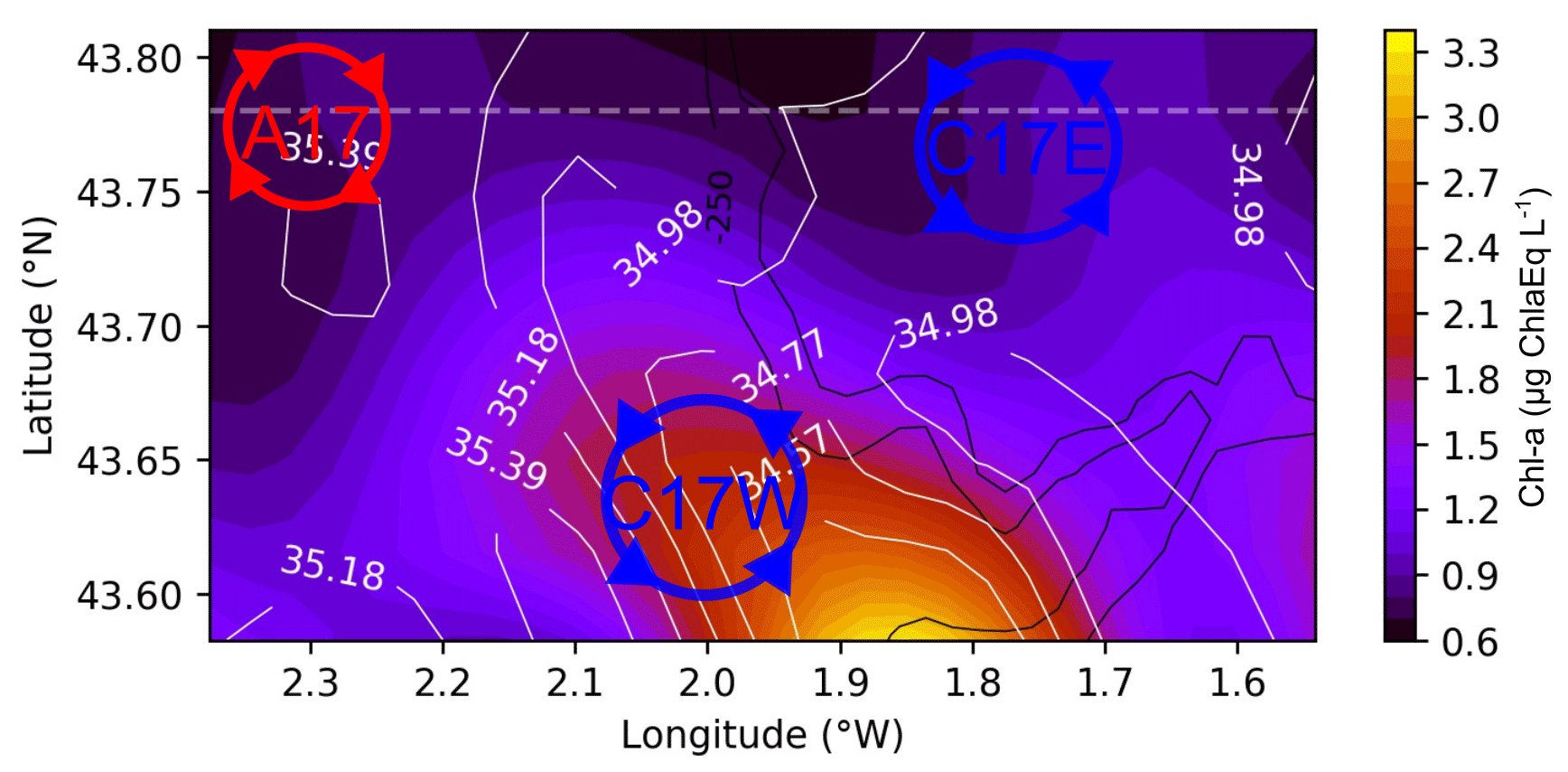
Figure 6 Surface chl a at 3.5 m from the surface Fluoroprobe for the period (2 to 4 August 2017). White contours represent the salinity field, while black contours represent the 200 and 250 m isobaths. The red (blue) circles in the left column represent the approximate location of A17 (C17W and C17E).

3.2 Chlorophyll a and spectral group distribution

Surface chl a (from the continuous recording surface Fluoroprobe) shows a distribution that is spatially dependent on salinity at 3.5 m depth, related to the position of the river plume (Fig. 6). The chl a maximum is observed around the salinity minimum, decreasing to the northwest (and with depth) in accordance with the increase of salinity. Vertically, the 43.77^∘ N cross section shows a complex distribution of total chl a and spectral groups (Fig. 7). Two DCMs are observed, one over the inner shelf at ∼ 30–50 m, and the second over the shelf edge at ∼ 50–65 m, which is below the pycnocline. The shallow DCM is split into two cores, although its morphology is hard to assess due to the limited spatial coverage of the sampling. The deep DCM is located at the anticyclonic frontal area between C17W and C17E and is composed of mainly brown algae, the dominant spectral group. The maximum is centred in the anticyclonic frontal area between C17W and C17E. Green algae, however, follow a different pattern and are distributed slightly deeper, following the salinity contours over 35.55. The ratio between brown chl a and green chl a (B : G), logarithmically transformed, provides an even clearer image of how the different spectral groups are distributed. There is a sharp transition between the brown algae (around the anticyclonic frontal area) and the green algae (below the 35.55 isohaline). The 43.70^∘ N cross section (see Fig. A2), which does not cross the core of the anticyclonic front, reveals that this pattern is not ubiquitous. Here, there is neither a clear dichotomy among the groups nor a deeper maximum of green algae.

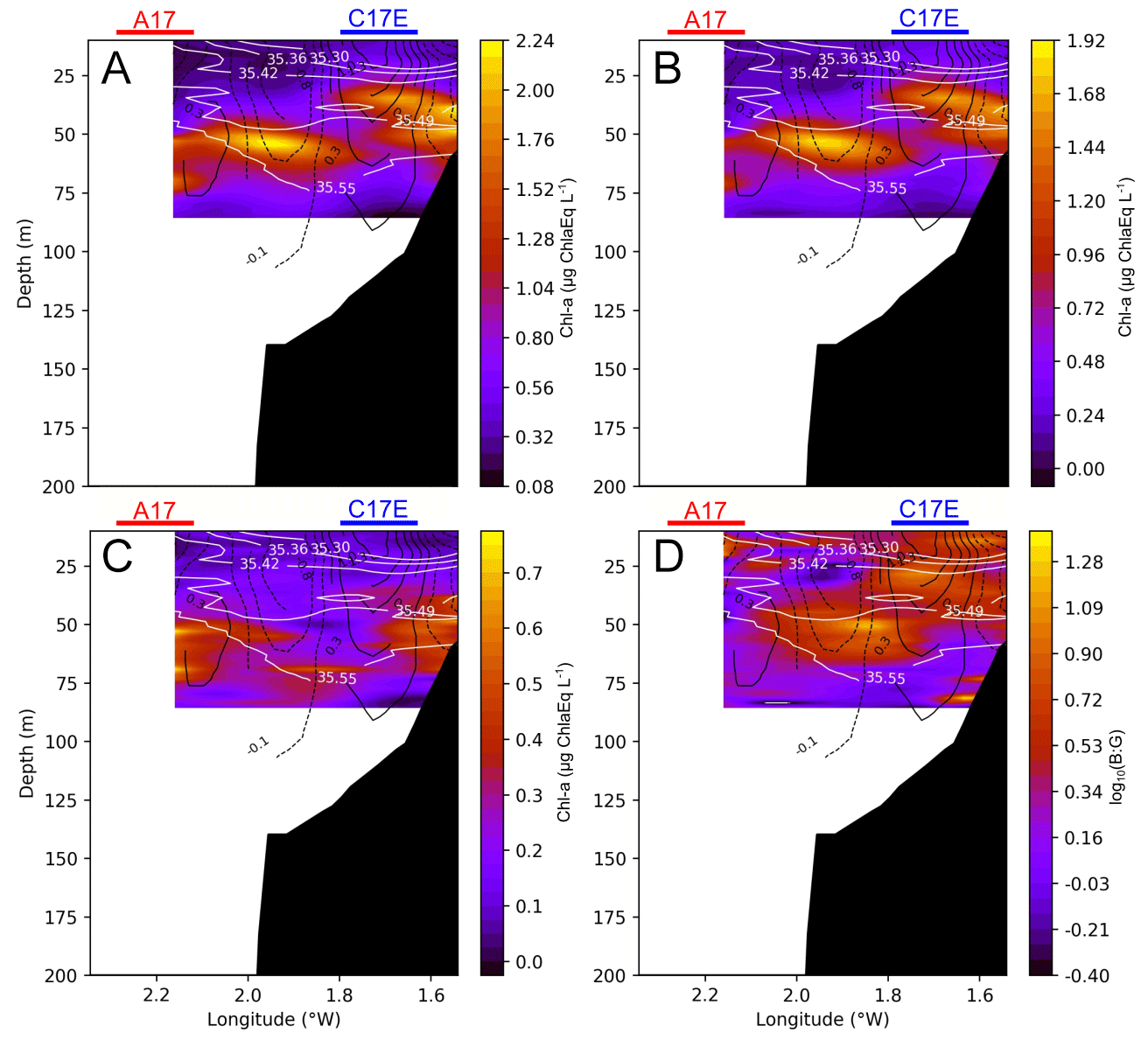
Figure 7 Cross section at 43.77^∘ N (location marked by dashed lines in Figs. 1 and 4; same section as in Fig. 5) of total chl a (a), brown chl a (b), green chl a (c), and the brown chl a to green chl a ratio (B : G), which has been logarithmically transformed (d) for the chosen period (2 to 4 August 2017). White lines represent salinity contours, and solid black lines represent positive vorticity values or cyclonic circulation, while dashed lines represent negative vorticity values of anticyclonic circulation. The red and blue horizontal lines represent the horizontal extension of A17 and C17E, respectively, that the section crosses.

Table 2 Variance contribution of the environmental variables to the estimated chl a concentrations for the different algae groups; brown : green (B : G) ratio; and the “above the pycnocline” (APY), “below the pycnocline” (BPY), and at the deep chlorophyll maximum (DCM) subsets. The left columns in each of the sections show these values for the models after stepwise deletion of the variables listed to the left (first the vertical velocities and then the temperature). The coefficient of determination (R²), general cross-validation score (GCV), and the percentage of variance (%) correspond to the different models. The last two models included only the variable listed (vorticity or salinity). For the right columns in each section, one variable (those listed on the left) was removed at a time while keeping the rest. While R² and GCV still refer to the whole model, percentage of variance is individual and corresponds only to the removed variable. Bold numbers point out the main modulating variable, i.e. the one that individually explains most of the variance in the model.

3.3 Exploring bio-physical impacts

The results of the GAMs in the APY subset (Fig. 8, Table 1) suggest that, overall, all of the models perform well, explaining in all cases more than 40 % of the variance. Salinity and temperature contribute to most of the variance of the model and explain 13.10 % and 9.8 % of it, respectively (Table 2). As expected, in agreement with Fig. 6, lower salinity values are associated with higher total chl a concentration, showing a negative relationship (Fig. 8a). Regarding the effect of temperature, it follows a convex-shaped function, with a minimum at ∼22 ^∘C (Fig. 8b), while the contribution of vorticity (Fig. 8c) is very small. The response of brown chl a differs from total chl a, although salinity still explains most of the variance of the model (23.3 %). Brown chl a shows a dome-shaped response to salinity (Fig. 8e) with a maximum at ∼ 35.1 (i.e. waters fresher or saltier than 35.1 have a negative impact) and a positive response to positive (cyclonic) vorticity. Green chl a almost mimics the distribution of total chl a (Fig. 8i–m), except for the non-significant relation with vorticity (p value > 0.05). For green algae, temperature and salinity explain 10.40 % and 12.70 % of the variance, respectively. Note that in this case the removal of salinity has no penalty in the explained variance, likely owing to the temperature capturing most of the variability. The B : G ratio shows dome-shaped relationships for salinity and temperature, where the maxima are at ∼ 35.2 and ∼ 22 ^∘C (Fig. 8n and l). In fresher and/or warmer waters, higher concentrations of green algae are observed. The contributions of both salinity and temperature to the variance are similar, i.e. 15.6 % and 15.8 %, respectively.

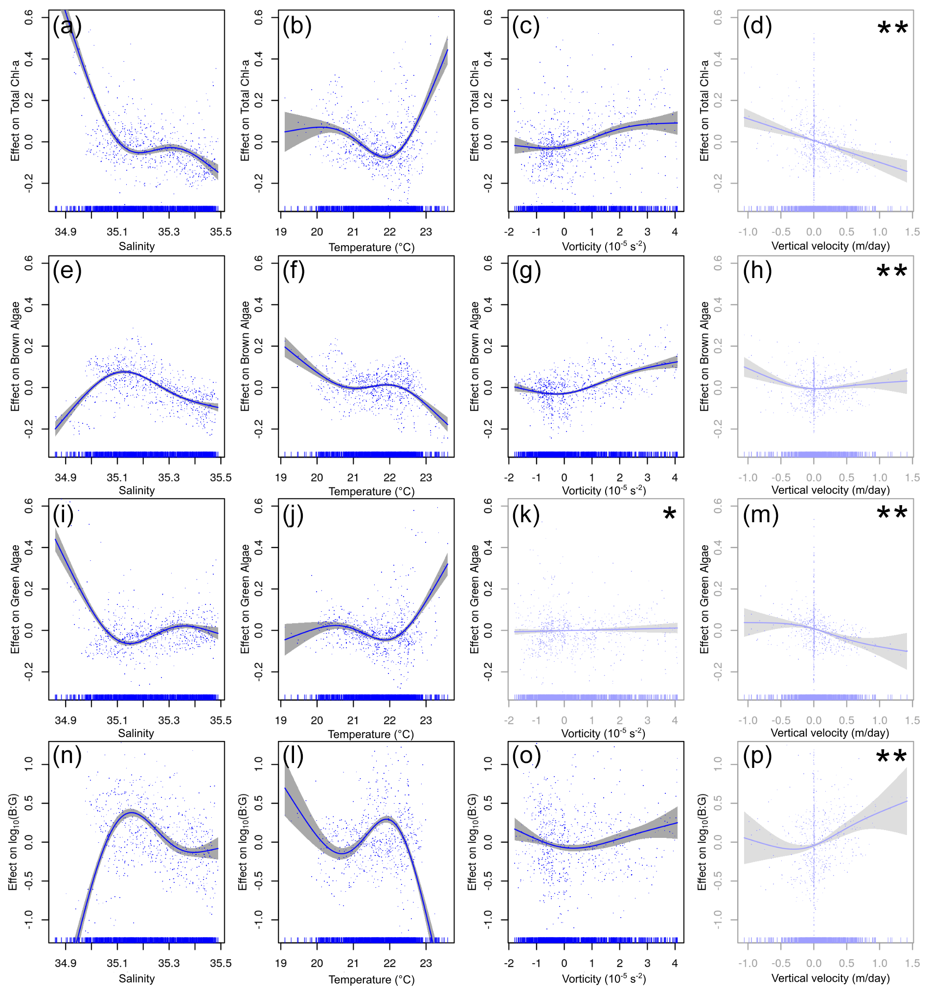
Figure 8 The relationship between environmental variables and chl a from the above the pycnocline (APY) subset GAMs. The y axis indicates the additive effect that the term on the x axis has on the chl a. The variables are given in the following order (from top to bottom): total chl a, brown chl a, green chl a, and the brown chl a to green chl a ratio (B : G). The shaded area represents the confidence interval of 95 %. The effect of vorticity for green algae chl a is the only non-significant response (marked by ^∗). The effect of vertical velocity is shown here but is not analysed further since this variable is strongly influenced (in the APY subset) by the proximity to the surface layer boundary condition assumed for its calculation (marked by ${}^{\ast \ast }$).

In the BPY subset, the GAMs explain a larger percentage of the variance and generally perform better than for the APY subset (except for the green algae) and suggest a different response of the chl a to the environmental variables (Table 1, Fig. 9). We observe a negative correlation between chl a and salinity until values of ∼ 35.5 (Fig. 9a) and a dome-shaped behaviour with temperature (34 % of explained variance), with a maximum at ∼ 14 ^∘C (Fig. 9b, Table 2). Although the explained variance by vorticity is small, there is a clear positive trend in chl a with negative or anticyclonic vorticity (Fig. 9c). Again, brown chl a mimics the responses of the total chl a (temperature explains most of the variance, 27.30 %). Green chl a shows a positive linear relationship with salinity (Fig. 9i) and a dome-shaped distribution with temperature (Fig. 9j, 19 % of explained variance), with a maximum at slightly colder waters. The B : G ratio (Fig. 9n) shows a negative correlation with salinity (11.80 % of explained variance), while temperature has a lower impact (4.50 % of explained variance).

While the GAMs at the DCM subset perform substantially worse for the total chl a (only 17.3 % of explained variance), they show much better performances for brown and green chl a distributions, with 37.7 % and 56.9 % of the explained variance, respectively. The model for the B : G ratio explains an even higher percentage of the variance (64.5 %). Total chl a distribution is correlated with salinity and vorticity (Fig. 10a and c) and shows a dome-shaped relationship with temperature (Fig. 10b) similar to that of APY and BPY subsets. However, the relative importance of the variables is different, vorticity explains the 9.97 % of the variance and is depicted as the main modulating environmental factor; however, this is very close to the 8.98 % explained by salinity. These differences are reinforced for the brown chl a model, where salinity and temperature explain a very low percentage of the variance (with almost flat distributions, Fig. 10e–f), and vorticity and vertical velocity are responsible of the 19.30 % and 4.40 % of the variance, respectively (Table 2). For the green chl a, the main modulating factors are salinity and vertical velocity (Fig. 10i and m, 25.40 % and 10.5 % of explained variance, respectively), while the effect of vorticity is very low (Fig. 10k, 4.10 %). In the case of DCM green chl a distribution, positive values of vertical velocity (upwelling) impact the chl a concentration negatively. Finally, for the B : G ratio, salinity stands out as the main modulating factor, explaining 20 % of the variance. However, the effect of vertical velocities and vorticity is also considerable, with 14 % and 9.30 % of explained variance, respectively.

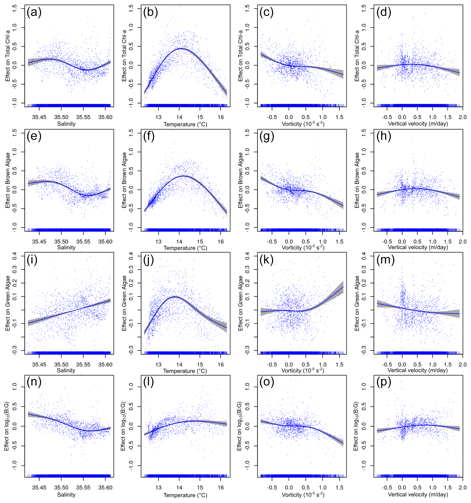
Figure 9 Relationship between environmental variables and chl a from the below the pycnocline (BPY) subset GAMs. The y axis indicates the additive effect that the term on the x axis has on the chl a. The following variables are shown (from top to bottom): total chl a, brown chl a, green chl a, and the brown : green (B : G) ratio. The shaded area represents the confidence interval of 95 %.

4 Discussion

During and around the dates of the ETOILE oceanographic cruise, two cyclones (C17W and C17E) were observed in the study area by means of different multiplatform sensors. While the signature of the cyclones in the HF radar fields was not continuous (and dependent on the prevailing wind conditions), their subsurface structure could be diagnosed from the hydrographic measurements obtained during the cruise. The geostrophic circulation indicated the presence of a dipole structure formed by C17W and C17E, a frontal region of anticyclonic circulation in between, and an additional anticyclone (A17). Further, two salinity fronts were observed, one near the surface (<14 m) and one at the subsurface (>50 m). From the chl a profiles, the DCM could be located below the pycnocline at ∼ 60 m, while the chl a distribution of the two dominant spectral groups of algae, brown and green algae, was depicted. The relative importance of the environmental factors modulating the chl a distribution was assessed by the use of GAMs. The GAMs not only showed that these environmental factors affect the brown and green algae differently but also that their relative importance changes throughout the water column. While salinity and temperature explain most of the variance above and below the pycnocline of both brown and green chl a, vorticity captures most of the variance in the DCM for brown algae.

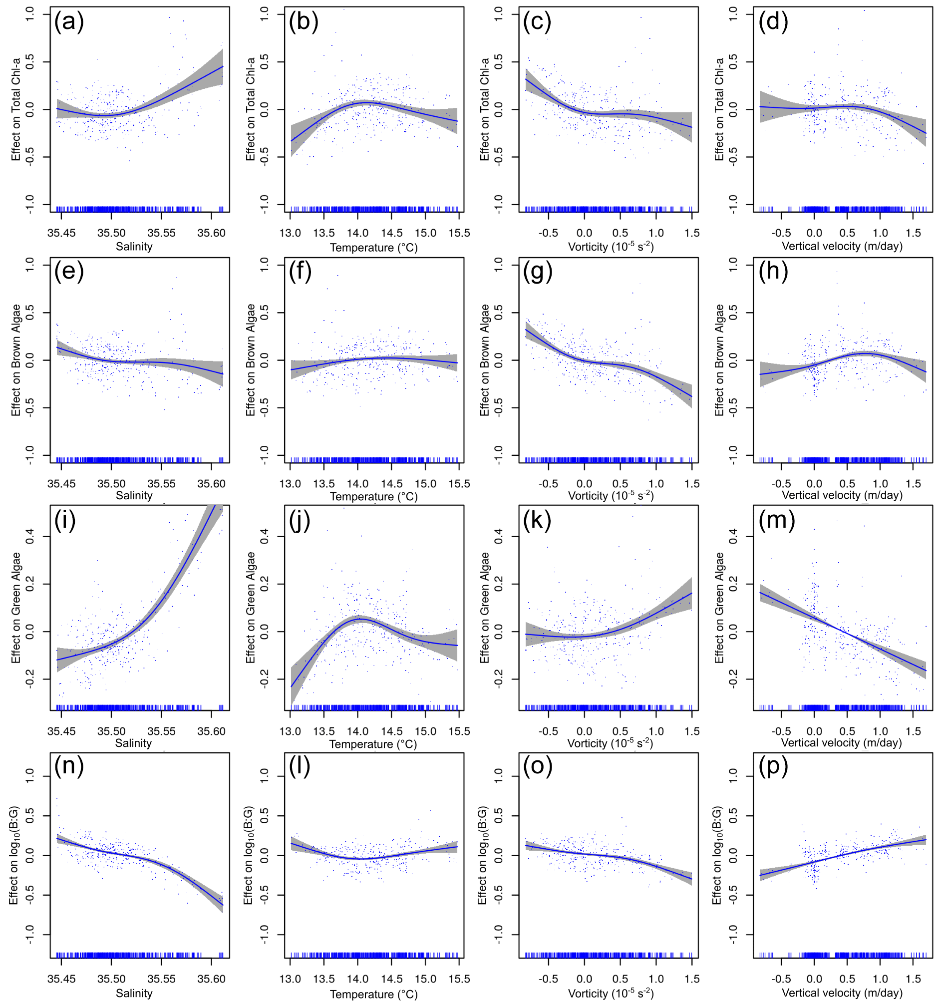
Figure 10 Relationship between environmental variables and chl a from the deep chlorophyll maximum (DCM) subset GAMs. The y axis indicates the additive effect that the term on the x axis has on the chl a. The following variables are shown (from top to bottom): total chl a, brown chl a, green chl a, and the brown : green (B : G) ratio. The shaded area represents the confidence interval of 95 %.

4.1 Physical environment

The hydrographic and hydrodynamic regimes observed at the SE-BoB during the ETOILE cruise, despite being spatio-temporally highly complex, were not exceptional and similar conditions have been already recorded. The surface salinity front we encountered onshore was observed on early May 2009 by Reverdin et al. (2013). They described a fresher (34–35) and deeper (∼ 30 m) freshwater layer originated due to winter and spring river runoff and which signal weakens towards August by increasing salinity to ∼ 35, as a result of vertical mixing and offshore advection by Ekman transport. This shelf break front is a recurrent feature in the study area, and is originated by the differences between the waters over the French shelf and the Landes Plateau and those located over the Spanish shelf and slope (Valencia et al., 2004).

Furthermore, the dipole-type structures have also been observed before in the BoB, yet in a larger scale (Pingree and Garcia-Soto, 2014; Solabarrieta et al., 2014; Caballero et al., 2016; Rubio et al., 2018). Both the location of the vertical velocities at the periphery of the structures and the magnitude (1–10 m d⁻¹) are consistent with already reported results (Mahadevan et al., 2008; Lévy et al., 2012; Caballero et al., 2016). While the cyclones were detected by the HF radar before the cruise, these were vanished during the survey due to the change in the wind-induced current regime. Their intermittent signature in the HF radar surface fields is explained by the interaction of the geostrophic and wind-induced flow. A similar situation was described using an analytical model in the Florida current by Liu et al. (2015), where a surface meandering flow was observed as a result of the overlap between a coastal jet and an eddy dipole field. This is coherent with our observations, i.e. under predominant NE winds the wind-driven circulation over the eddy field results in a meandering structure. Indeed, as the wind weakens the cyclones signature is again observed in the HF radar fields, highlighting the importance of using a wide range of multiplatform spatio-temporal data for a better characterization of the coastal hydrodynamics.

4.2 Environmental drivers

In the BoB, coastal chl a is highly dependent on the seasonality of riverine nutrient inputs (Guillaud et al., 2008; Borja et al., 2016; Muñiz et al., 2019). From satellite imagery and continuously recorded surface salinity and chl-a^sat data (Figs. 3 and 6), it is evident that the Adour and Bidasoa plumes are associated with the highest chl a concentrations at the sea surface. Simultaneously, the location of the Adour and Bidasoa plumes depends on the wind conditions, which control the non-geostrophic surface circulation, as shown by the HF radar LRC. Our results agree with the observed general pattern in which westerly winds push the river plume towards the coast, while easterly winds promote an offshore expansion (Petus et al., 2014). Thereby, the uppermost chl a pattern is eventually dependent on the winds that modulate the position of the river plume. At the subsurface, the occurrence of the DCM agrees with previously described phytoplankton distributions. Muñiz et al. (2019) described a DCM below 30 m in summer at the same sector on the BoB. Caballero et al. (2016) also reported a summer DCM at around 40 m (below the thermocline) at the periphery of two cyclones.

Between the uppermost layer and the pycnocline, non-geostrophic processes related to wind-driven currents (e.g. offshore advection of coastal waters during upwelling-favourable winds) have an important role in the chl a distribution changes, showing decreasing intensity with depth. In contrast, below the pycnocline, we could expect geostrophic currents to progressively become the main driver for particle advection. These two layers are also different regarding the nutrient supply. Typically, waters above the mixed layer are depleted in nutrients, whereas below this point the phytoplankton would benefit from the nutrient supply via ocean deep waters in combination with maximum light penetration in summer (Cullen, 2015). This can also lead to different phytoplankton communities with different nutrient requirements.

At APY, most of the variance of total and brown chl a is explained by salinity, while the environmental variable that explains most of the green chl a variance is temperature. These results suggest that the green algae is likely associated with the presence of nutrients on river plumes (fresher and warmer waters) from Adour and Bidasoa. However, the brown algae seemed to be unaffected by the river plume, at least directly, since they display high chl a concentration at deeper, colder, and slightly saltier waters. The causative link between the environmental variables and the brown chl a distribution is harder to draw. However, salinity is the main modulating factor and might suggest an indirect link with nutrient provisioning by river runoff. At BPY, temperature is the variable that explains most of the variance. However, this could be the result of the positioning of the DCM at a specific depth and the large vertical gradient of temperature in the water column, where there would be a good compromise between light and nutrient availability (not measured during this study) for phytoplankton growth (Cullen, 2015). In fact, for the B : G ratio, this effect cancels out, and salinity is the most important environmental factor. Overall, when integrating the entire water column, even though the responses differ in the different subsets, salinity is the most important environmental factor regarding the total chl a distribution and the relative occurrence of brown and green algae. We attribute this effect to salinity and its relation to nutrient content at the surface (with fresher water) and at depth (saltier waters) (Muñiz et al., 2019).

At the DCM, vorticity is the factor that explains most of the variance in total chl a and brown chl a concentrations. The more negative (positive) the vorticity, the more anticyclonic (cyclonic) the circulation and the more positive (negative) the effect on brown chl a concentrations. In anticyclones, due to Ekman transport, a small part of the flow targets the core, leading to an accumulation of phytoplankton at their centre (Mahadevan et al., 2008). In contrast, Ekman transport results in outward transport in cyclones. Therefore, C17W and C17E would have advected the brown algae and expelled them from the core. These were then subsequently trapped in the anticyclonic circulation located between the cyclones. A similar pattern is described by Caballero et al. (2016), where the highest chl a concentrations were located at the periphery of the cyclones. The effect of this advection by submesoscale processes is such that the distribution of brown algae at the DCM cannot be statistically explained without the addition of vorticity to the GAM.

However, the distribution of green chl a is not affected by vorticity, and the environmental factor that exerts most of the difference between the two spectral groups is salinity. From our observation we cannot explain the occurrence of a single spectral group in the core of the anticyclonic circulation. Latasa et al. (2017) demonstrated that, during the summer stratification in the Iberian Shelf and Iberian Margin, the DCMs are composed of different types of phytoplankton, each adapted to the different existing micro-environments. However, the phytoplankton landscapes organized in submesoscale patches are often dominated by a single species (D'Ovidio et al., 2010). This structuring of the phytoplankton community is a direct effect of the horizontal stirring, which can create intense patchiness in species distribution (Lévy et al., 2012). We believe that the observed submesoscale processes during the ETOILE cruise would have perturbed an already existing horizontal layer of DCM, not enhancing primary production (not measured during our study) by themselves but rather isolating, advecting, and gathering the phytoplankton in the region of anticyclonic circulation.

4.3 Limitations of this study

It is worth stating the main limitations encountered during this study, especially focusing on the ETOILE cruise. The sampling area was insufficient to completely cover some of the observed structures. Similarly, having just a synoptic image of the processes and lacking temporal information (despite operational and remote sensing data) makes it challenging to derive a cause–consequence relation, especially regarding the evolution of the system. Although we used chl a as a proxy for phytoplankton biomass concentration, we note that photo-acclimation of pigment content (Cullen, 2015), together with variable fluorescence to chlorophyll ratios (Estrada et al., 1996; Kruskopf and Flynn, 2006; Houliez et al., 2012), could lead to elevated chl a concentration relative to phytoplankton biomass at depth.

In addition, no further phytoplankton classification was carried out, which might have helped in defining specific environmental niches (D'Ovidio et al., 2010; Latasa et al., 2017) and correlating spectral groups to pigmentary groups and/or taxa. The latter is an essential issue to be considered, since the Fluoroprobe factory fingerprints are determined on mono-specific cultures or target micro-algae that are not necessarily representative to our shelf and ocean system (Houliez et al., 2012). No nutrient or light measurements were taken either; therefore, we cannot explicitly describe any inter-species competition, which would have helped us in understanding the ecological consequences of these submesoscale processes. A distinct spectral community structure was still detected, when compared to the surrounding waters, which could potentially be extended through the trophic web and even affect predator foraging behaviour (Cotté et al., 2015; Tew Kai et al., 2009). Thus, our results suggest that the combined effects of submesoscale features, even though they concern a relatively small fraction of the total area, may be disproportionately important to biological dynamics.

5 Conclusions

We analysed multi-platform in situ and remote sensing data to characterize coastal submesoscale processes and their influence on the distribution of the two major phytoplankton pigmentary groups in the SE-BoB. Satellite imagery and HF radar data provided information about the uppermost layer, which was highly conditioned by the run-off of Adour and Bidasoa rivers. The location of the plume was influenced by the surface currents, which are ultimately conditioned by the speed and direction of the wind.

Multi-spectral chl a fluorescence measurements allowed us to identify the contrasting effects of a set of environmental variables on the distribution and concentration of different phytoplankton spectral groups. From top to bottom, salinity explained most of the distribution of the chl a for both brown and green algae. While salinity would still be the most important environmental driver for green algae at the DCM, vorticity explained most of the variance of the distribution of total chl a and brown chl a at this layer. Anticyclonic circulation gathered the brown algae in the centre via Ekman transport. The effect was such that the distribution of brown algae within the DCM could not be statistically explained without the vorticity as an environmental variable. This research brings the relevance of the dynamic variables in the study of phytoplankton into consideration, as well as the measurements of multi-spectral chl a fluorescence at high spatial resolution. Further research providing a more detailed composition of the phytoplankton community in terms of pigments, size classes, and taxonomy, together with an exhaustive analysis of the hydrodynamics, will help to better identify the ecological and functional traits of phytoplankton groups and determine their submesoscale distribution in coastal systems.

Appendix A

A1 Observation of eddies after ETOILE

After the change in wind regime on 7 August, the eddy C17W is again visible in the HF radar. It has moved southwards with respect its location on 29 July. Meanwhile, C17E has vanished, although it might only be masked by the surface currents since a meandering is still visible in its former location at 1.7^∘ W.

Figure A1 Lagrangian residual currents (LRC) for the period of 6 to 9 August, the persistent C17W eddy is still visible after the change in wind regime.

A2 Phytoplankton observations at T3

A cross section at the 43.70^∘ N out of the core of the anticyclonic frontal area, revels that this pattern is not ubiquitous. Here there is not a clear dichotomy among the groups nor a deeper maximum of green algae. Rather, there is a uniform layer of brown algae.

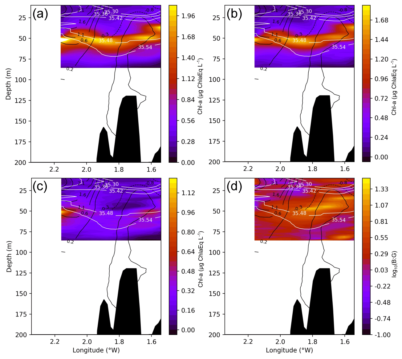
Figure A2 Cross section at 43.70^∘ N of total chl a (a), brown chl a (b), green chl a (c), and the brown : green (B : G) ratio logarithmically transformed (d). White lines represent salinity contours and solid (dashed) black lines represent positive (negative) vorticity values or cyclonic (anticyclonic) circulation.