the Creative Commons Attribution 4.0 License.
the Creative Commons Attribution 4.0 License.
 | 04 Jun 2021
A new Lagrangian-based short-term prediction methodology for high-frequency (HF) radar currents
Lohitzune Solabarrieta
Ismael Hernández-Carrasco
Anna Rubio
Michael Campbell
Ganix Esnaola
Julien Mader
Burton H. Jones
Alejandro Orfila
The use of high-frequency radar (HFR) data is increasing worldwide for different applications in the field of operational oceanography and data assimilation, as it provides real-time coastal surface currents at high temporal and spatial resolution. In this work, a Lagrangian-based, empirical, real-time, short-term prediction (L-STP) system is presented in order to provide short-term forecasts of up to 48 h of ocean currents. The method is based on finding historical analogs of Lagrangian trajectories obtained from HFR surface currents. Then, assuming that the present state will follow the same temporal evolution as the historical analog, we perform the forecast. The method is applied to two HFR systems covering two areas with different dynamical characteristics: the southeast Bay of Biscay and the central Red Sea. A comparison of the L-STP methodology with predictions based on persistence and reference fields is performed in order to quantify the error introduced by this approach. Furthermore, a sensitivity analysis has been conducted to determine the limit of applicability of the methodology regarding the temporal horizon of Lagrangian prediction. A real-time skill score has been developed using the results of this analysis, which allows for the identification of periods when the short-term prediction performance is more likely to be low, and persistence can be used as a better predictor for the future currents.
- Article
(3380 KB) - Full-text XML
- BibTeX
- EndNote


The coastal zone is under increasing human pressure. During recent decades coastal seas have been experiencing intensified activity for recreation, transport, fisheries, and marine-related energy production, which, in many cases, results in serious damage to coastal marine ecosystems. A better understanding of the dynamical processes responsible for the surface oceanic transport is a prerequisite for the efficient management of the coastal ocean. Coastal processes are responsible for the transport and fate of multi-source pollutants like plastics, nutrients, jellyfish, and harmful algal blooms. Thus, improving the capacity of monitoring and forecasting the coastal area is key for the integrated assessment of the marine ecosystem. This requirement is driving the setup of a growing number of multi-platform operational observatories designed for continuous monitoring of the coastal ocean from international or national (e.g., US IOOS, EU EOOS, Australian IMOS) to local scales. Moreover, due to the need for forecasting applications for response to emergency situations such as oil spills or search-and-rescue operations, many of the existing operational observatories are linked with operational ocean forecasting models with or without data assimilation (e.g., MARACOOS, NOAA Global Real-Time Ocean Forecast System, COPERNICUS Marine Environment Monitoring System).
With the need to provide a long-term framework for the development and improvement of European marine coastal observations, the JERICO Research Infrastructure (JERICO-RI) has been developing methods and tools (through the JERICO, JERICO-NEXT, and JERICO-S3 projects) for the production of high-quality marine data and sharing expertise and infrastructures between the existing observatories in Europe. Typically constituted with different in situ pointwise observational platforms (such as moored buoys, tidal gauges, and/or drifting buoys), a significant number of these observatories now employ land-based high-frequency radars (HFRs) that provide real-time coastal currents with unprecedented coverage and resolution (e.g., Paduan and Rosenfeld, 1996; Kohut and Glenn, 2003; Abascal et al., 2009; Solabarrieta et al., 2014; Rubio et al., 2017; Paduan and Washburn, 2013). Each HFR coastal site measures radial surface currents moving away from or approaching the antenna based on the shift of the first peak (Bragg peak) of the Doppler spectra (Crombie, 1955; Barrick, 1977). Combining the overlapping radial vectors from at least two antennas provides surface true vector currents (Barrick et al., 1979; Barrick and Lipa, 1979). Several studies have compared in situ current measurements with HFR observations (e.g., Schott et al., 1985; Hammond et al., 1987; Paduan and Rosenfeld, 1996, Emery et al., 2004; Paduan et al., 2006; Ohlmann et al., 2007; Liu et al., 2014; Solabarrieta et al., 2014; Bellomo et al., 2015; Lana et al., 2016; Hernández-Carrasco et al., 2018b) and have repeatedly demonstrated the potential of this technology. Presently, more than 250 HFR antennas are installed and active worldwide (Roarty et al., 2019; http://global-hfradar.org/, last access: 26 May 2021).
Due to their high spatiotemporal resolution, HFR data are commonly used in real time for search-and-rescue (Ullman et al., 2006) or oil spill prediction and mitigation emergency response (Abascal et al., 2017). In addition, there have been several efforts dedicated to the development of assimilation strategies that incorporate HFR-measured surface currents into ocean coastal models (Breivik and Saetra, 2001; Oke et al., 2002; Paduan and Shulman, 2004; Stanev et al., 2011; Barth et al., 2011), some of which have been tested for short periods of time (Chao et al., 2009). However, assimilation of HFR data into models is still a computationally expensive and complex issue, not to mention the operational capabilities of such a procedure. Because of these constraints, the availability of real-time high-resolution HFR current fields has led to alternative solutions in order to obtain short-term prediction (STP) of surface coastal currents through the direct use of HFR historical and nowcast observations using different approaches (e.g., Zelenke, 2005; Frolov et al., 2012; Barrick et al., 2012; Orfila et al., 2015; Solabarrieta et al., 2016; Vilibić et al., 2016; Ren et al., 2019; see Table 1).
Table 1Characteristics of the previously developed STP works based on HFR data.
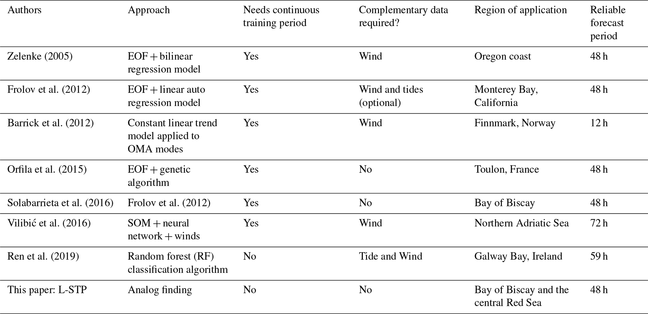
The abovementioned studies develop and implement different STP approaches (harmonic analysis of the last hours, genetic algorithms, numerical models) that often require either additional data or long training periods of data without gaps. Hardware failures due to power issues, communications, or environmental conditions often result in spatiotemporal gaps within HFR datasets. Spatial gaps can be filled on a real-time basis, but filling long temporal gaps is not straightforward. Several gap-filling methodologies have been developed for HFR datasets: open modal analysis, (OMA) (Kaplan and Lekien, 2007), data-interpolating empirical orthogonal functions (EOFs) (DINEOF) (Hernández-Carrasco et al., 2018a), and self-organizing maps (SOMs) (Hernández-Carrasco et al., 2018a).
Given the motivation described above, and developed partially within the framework of the JERICO-NEXT project, we present a Lagrangian-based short-term prediction (L-STP from now on) methodology using existing HFR datasets to be applied to surface current real-time observations. The proposed L-STP methodology aims to be capable of using the previously developed gap-filling OMA method and generate forecasts in near-real time with low computational costs compared to previously presented forecast methods, but with the same level of assessment. The uniqueness of this approach is twofold: first, the historical Eulerian velocity fields are used to construct a catalog of Lagrangian trajectories, and second, using the trajectories obtained from present observations, analogs in the past dataset are searched in order to obtain the best predictive match. The method is based on Lagrangian computations, which have proven to be robust against errors in velocity field data and against the dynamics of unresolved scales, since the averaging effect produced by integrating over trajectories that extend in time and space tends to cancel random-like errors (Hernández-Carrasco et al., 2011; Sayol et al., 2014). Consequently, they are reliable for the assessment of dynamical flow structures.
Analogs represent a widely used method in time series prediction, especially in early weather forecasting and statistical downscaling. This is based on the assumption that if the behavior of a dynamical system at a given time is similar or close enough to some other situation in the historical record, then the evolution in the future of the state of the system will be similar to the evolution observed in the same historical record. Simply stated, two analog fields are two distinct fields that are close enough considering a given metric to be considered equivalent. Finding the best (nearest) analog of a specific time does not require a historically continuous dataset as long as the dataset contains subsets of observations that extend longer than the testing period and are representative of the range of potential states that the system can have. These statistically analog events occur naturally in the environment, and this methodology has been applied and tested in atmospheric forecasts (Lorenz, 1969; Jianping et al., 1993; Prince and Goswami, 2007; Shao and Li, 2013).
It must be stressed that this is the first time that the analog technique has been applied to the HFR-derived ocean surface currents to obtain short-term forecasts to the knowledge of the authors. The L-STP is intended to be implemented operationally with low computational cost (seconds to few minutes for each forecast, depending on the size of the historical dataset) and is easily implemented using existing HFR data processing tools.
2.1 Data
HFR data from two distinct oceanographic regions have been used for the evaluation, validation, and testing of the developed methodology (Fig. 1): the Bay of Biscay (hereinafter BoB HFR) and the central Red Sea region (hereinafter Red Sea HFR). The range and the spatial resolution of the HFR current systems depend on their working frequency and the conductivity of the water over which the system is measuring. Ranges vary from 15 to 220 km and spatial resolution from 250 m to 12 km. Typically, a 12 MHz radar has a range of ∼ 70 km with a spatial resolution of 2–5 km. HFR systems usually average current measurements for 1 h, although some average currents for shorter periods, such as 30 min. HFR data from these two regions are used to evaluate the skill of the method under different dynamical conditions and with a sufficient set of observations to provide a database suited to the efficient research of appropriate analogs. The BoB HFR system, located in the southeastern corner of the Bay of Biscay in the Basque Country, is composed of two CODAR SeaSonde sites working since 2009 at 4.5 MHz frequency, covering up to a 200 km range, and providing hourly surface velocity fields at 5 km of spatial resolution. The dataset used in this study spans the period from January 2012 to December 2015. The Red Sea HFR system is located on the central western coast of Saudi Arabia and is also composed of two CODAR SeaSonde sites. The Red Sea sites have been operational since June 2017, transmit at a 16.12 MHz frequency, cover up to a 120 km range, and provide the hourly surface velocity field at 3 km spatial resolution. The dataset used in this study spans the period from June 2017 to October 2018.
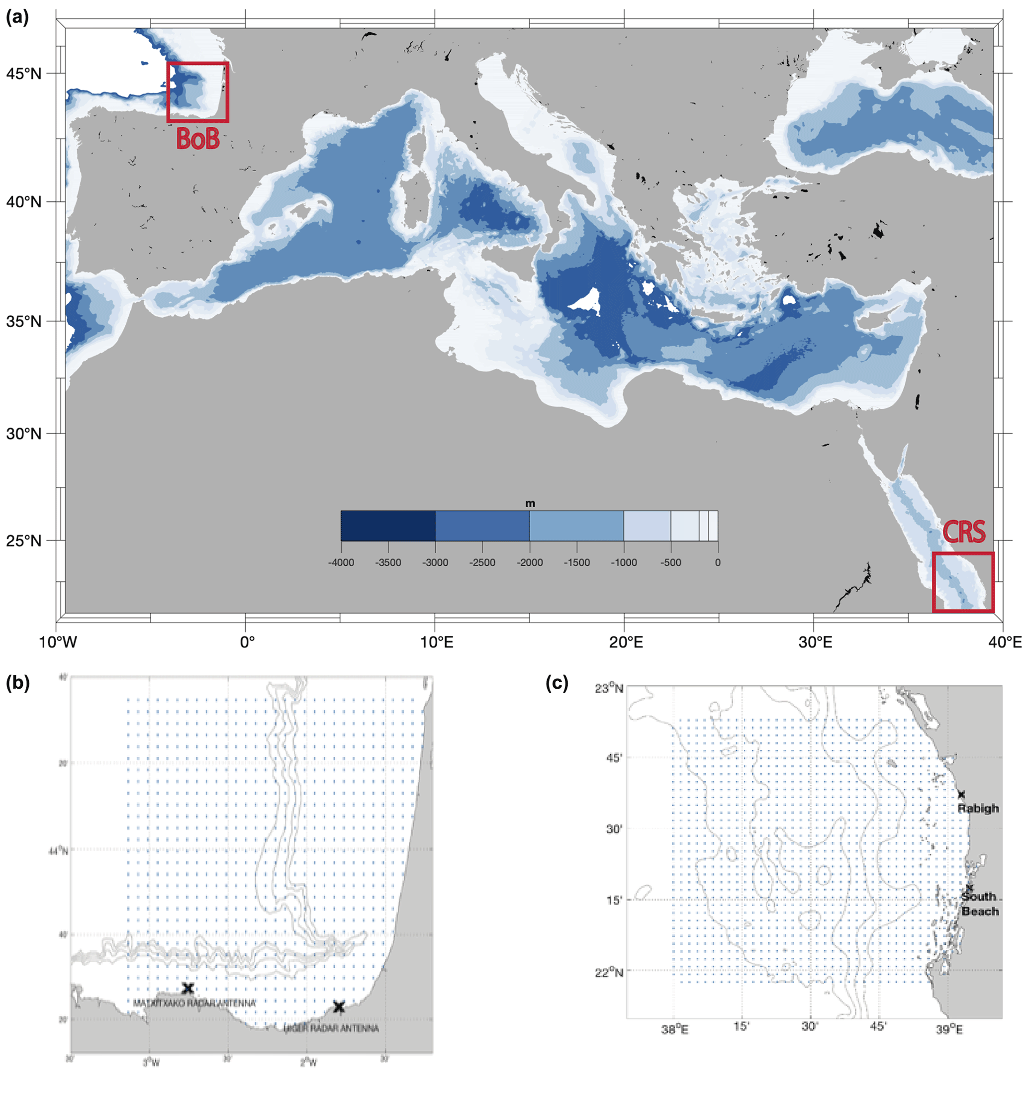
Figure 1(a) A global view of both analyzed study areas. (b) HFR system of the BoB. (c) HFR system of the central Red Sea. Blue dots represent the data points, and the black crosses are the HFR antenna positions.
The BoB HFR has been chosen as the pilot system for testing the developed methodology, since it has the longest data series and because several papers have already provided an extensive description of the local circulation and dynamical processes (Rubio et al., 2013a, b, 2018, 2019, 2020; Solabarrieta et al., 2014, 2015; Hernández-Carrasco et al., 2018a; Manso-Narvarte et al., 2018; Declerk et al., 2019). The resulting methodology is then applied to the operational Red Sea HFR dataset as a study case. Coastal dynamics in the BoB show a clear seasonality, with cyclonic and anticyclonic eddies dominating in winter and summer, respectively, in responding to local winds and the mean coastal current (Iberian Poleward Current) (Esnaola et al., 2013; Solabarrieta et al., 2014). The circulation in the central Red Sea also demonstrates a clear seasonality (Sofianos and Johns, 2003; Yao et al., 2014a, b; Zarokanellos et al., 2017a, b) linked to the seasonal winds of the area (Abualnaja et al., 2015; Langodan et al., 2017). The region is dominated by eddy activity, with both cyclonic and anticyclonic eddies occurring in the region (Zhan et al., 2014; Zarokanellos et al., 2017a). Due to the only recently available dataset (since mid-June 2017 to present) the detailed small-scale surface circulation processes of this area are under characterization at the moment.
The primary difference between the two HFR systems is the operating frequency, resulting in larger spatial coverage for the BoB HFR than for the Red Sea HFR and a higher spatial resolution for the latter (5 and 3 km, respectively). This difference in the spatial resolution should result in better capturing the small-scale dynamical features in the Red Sea, which could influence the selection of an analog.
The data from both systems have been processed similarly. The spectra of the received backscattered signal are converted into radial velocities using the MUltiple SIgnal Classification (MUSIC) algorithm (Schmidt, 1986). The HFR_Progs MATLAB package (https://github.com/rowg/hfrprogs, last access: 26 May 2021) is then used to combine radial currents and generate gap-filled total 2D currents by means of the open modal analysis (OMA) methodology of Kaplan and Lekien (2007).
2.2 Lagrangian analogs
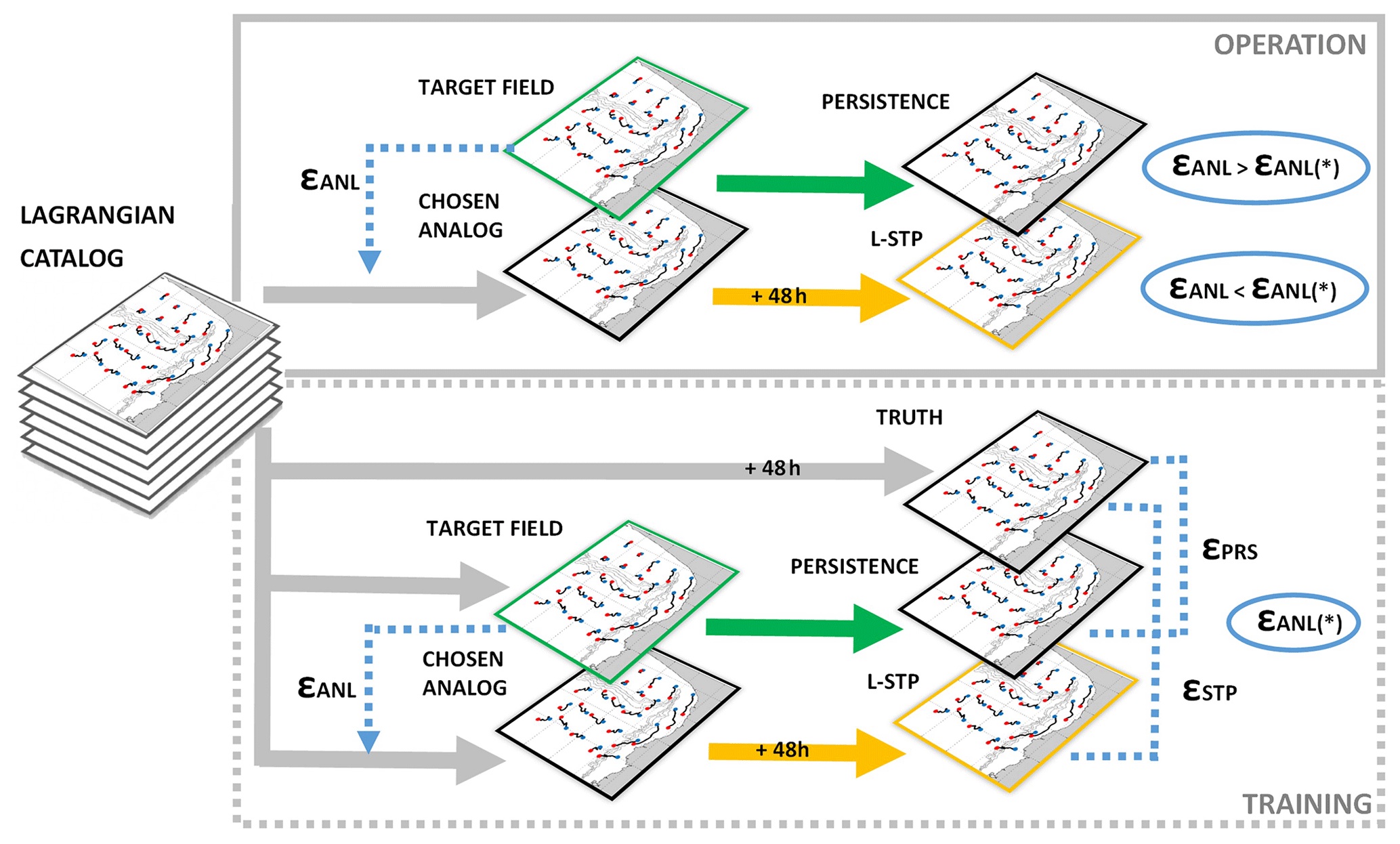
The proposed prediction system, based on the analog identification method, has been developed with the objective of providing HFR velocity field forecasts (up to 48 h). As an innovative element, we use a Lagrangian approach in searching for analogs through a historical library composed of particle trajectories instead of the commonly used Eulerian velocity fields. In our methodology we find the best analog by comparing maps of trajectories obtained from the last available 48 h (target field) with the historical catalog of maps of Lagrangian trajectories (hereinafter Lagrangian catalog). Then the catalog map with the trajectory pattern closest to the target field map is selected. Relying on the similar evolution of the current situation and the past analog, the next 48 h time velocity fields of the selected analog provide the target period forecast. In other words, if we find a state in the historical database that is “close enough” to the target field, we assume that the forecast for the current observations will evolve in the same way as for the chosen analog. A detailed description of the short-term prediction system is provided in the following algorithm.
-
Lagrangian catalog configuration. First, to build the Lagrangian catalog, a set of synthetic trajectories was computed by advecting N particles uniformly initialized on a regular grid (Fig. 2) in the OMA HFR velocity fields. The N Lagrangian particles are released every hour over all available velocity data and advected during 48 h. The maps of trajectories of the catalog are referred as to XC.
-
Target map. A map of trajectories corresponding to the most recent HF currents observations, referred as to XT, is computed using the same procedure as for the Lagrangian catalog but now advecting the N particles in the last available 48 h (tf–48 h) of HFR velocity fields, where tf corresponds to the current time.
-
Searching for the analog. A searching algorithm for the best (closest to the target map) analog among all the trajectory maps is implemented next. To increase the efficiency of this process, the search was done in two steps.
- i.
Optimization of the catalog. First, selecting only “potential” analogs with a similar main drift reduces the Lagrangian catalog. The trajectory centroid for each map of the catalog is computed and compared to that of the target field, finally discarding the analogs whose centroid was at a distance greater than δcg. The value of the δcg is selected to be small enough to minimize the computational time but sufficiently large not to lose sampling variability in the potential analogs. We explored different values of this threshold distance to find that km (where ξ is the spatial resolution) makes a good compromise between computational cost and the number of potential analogs in both study areas.
- ii.
In a second step, we computed the Lagrangian errors (ε) between the trajectories of the target field and the potential analogs, defined as
where T=5 is the number of elements of the set of times ti, and δANL (ti) is the mean separation distance at time ti between the trajectories belonging to the target field XT and each of the potential analogs Xc, given by
with N being the total number of trajectories j.
- i.
-
Best analog. The selection of the best analog is performed by Eq. (1), which is a simple measure of similarity between two datasets. The best analog is selected as the element of the catalog with the lowest εANL. Figure 3 shows an example of the time series of εANL values through the catalog of potential analogs for a specific case. Then we locate the time tANL corresponding to best analog: tANL→ min(εANL) = εANL(tANL):Xc(tANL).
-
Current prediction. Once we have identified tANL, the short-term forecast of the HFR velocity fields is given by the hourly velocity fields corresponding to the next 48 h since tANL (hereinafter “L-STP fields”):
where VC (tANL) is the velocity field corresponding to the best analog and VSTP represents the forecast currents.
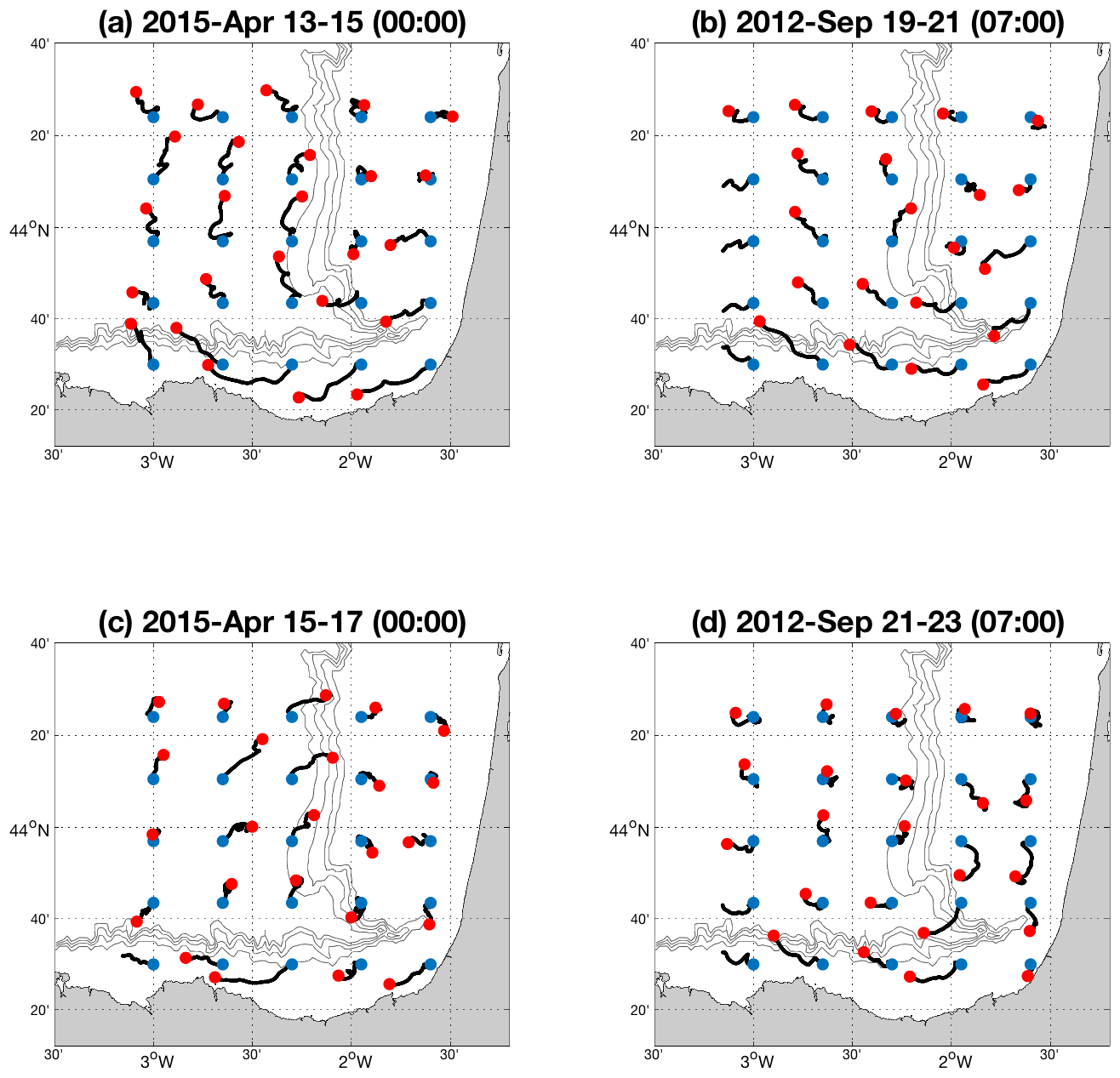
Figure 215 April 2015 00:00 example of the developed methodology applied to the BoB HFR system. (a) The past 48 h of the target field for the test period. (b) The analog having the lowest error. (c) The truth trajectories for the forecast period. (d) The STP trajectories. The initial positions of the particle trajectories are indicated by the blue dots, and the red dots indicate the position after 48 h.
Figure 2 provides an example of the selected analog (Fig. 2b) and corresponding L-STP fields (Fig. 2d) for a given target field (Fig. 2a) and the “truth” trajectories for the following 48 h from the date of the target field (Fig. 2c). The associated temporal series of errors for the target field and the potential analogs are shown in Fig. 3, where the value of εANL is marked using a red dot (corresponding to the error between the trajectories of the L-STP field in Fig. 2d and the truth trajectories for the forecast period in Fig. 2c).
To assess the performance of the methodology, we computed forecasted trajectories based on the persistence of currents (hereinafter “persistence fields” XPRS). To obtain simulated trajectories using persistence currents, the particles are advected during 48 h using a constant (frozen) velocity field (given by the current velocity field, or target field, V(tf)) during the 48 h of simulation: , where tf is the current time and .
The mean drift of the truth forecasted trajectories, XTRU, is also computed for each simulation period (the mean drift is computed by averaging over the entire particle trajectory length during 48 h).
The Lagrangian errors between the truth trajectories XTRU and the L-STP trajectories XSTP were also computed as
where δSTP is the mean separation distance between the truth and the L-STP trajectories for (following 48 h from the study time). To compare with persistence, we also compute the Lagrangian error between the truth trajectories XTRU and the trajectories derived from the persistence field XPRS,
where δPRS is the mean separation distance between the truth maps of trajectories, XTRU, and maps of trajectories from persistent velocity fields, XPRS, for (following 48 h from the study time).
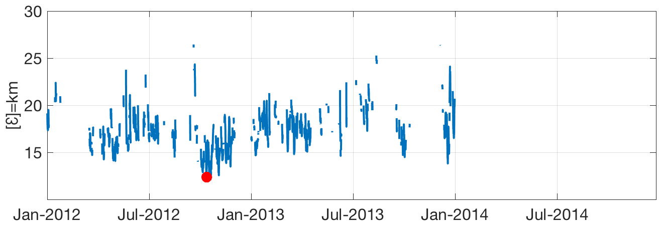
Figure 3Example for the test period on 15 April 2015 at 00:00; errors are for all Lagrangian catalog fields of the BoB HFR system (training period 2012–2014), restricted to the δcg=10 km condition. The red dot indicates the occurrence date and the error of the best analog (19 September 2012 at 07:00).
The entire process for the selection and validation of the analog with the different variables has been summarized in Fig. 4. The time series and spatial distribution of the εSTP and εPRS errors have been analyzed for both study areas. Finally, εSTP and εPRS time series have also been calculated and compared to the time series of the εANL in order to evaluate if the εANL can be used as an indicator of the expected skill of the L-STP with respect to the persistence.
Some parameters in the algorithm have to be tuned in order to optimize the results and the computational cost. For instance, we found that the optimal number of particle trajectories, N, is equal to 25. All the trajectories have been computed considering infinitesimal and passive particles without adding a diffusion term. To this end, we used the Lagrangian module included in the HFR_Progs MATLAB package.
The ability of this method relies on precision in finding two matching HFR current states over the entire region, which is dependent on the historical record of observations used to build the catalog and the dynamical representativity of the catalog. In this study we use a 4-year dataset (2012–2015) of trajectory maps computed for the SE BoB; the trajectory maps from the first 3 years (2012–2014) were used as a Lagrangian catalog, and the remaining year (2015) was used as a test period. The historical Lagrangian catalog for this HFR system is thus composed of 26 304 maps of N=25 trajectories of 48 h. Then the method was applied to the Red Sea dataset for the period of July 2017–October 2018. As the dataset temporal extension was short (1 year and 4 months), we have used the whole period to build the Lagrangian catalog to act as a test period at the same time. In this case, for the analog search the 5 d period around the date of the target field was removed from the catalog at each iteration to avoid temporal overlapping with the target field.
Figure 2 shows an example of the developed methodology applied to the BoB HFR system on 15 April 2015. It is a visual representation of the (a) target trajectories, (b) the selected analog, (c) truth trajectories during the next 48 h from the target period, and (d) the L-STP trajectories provided by the method (48 h from the analog).
The performance assessment results are described in Sect. 3.1, and the temporal and spatial forecasts for both study areas are shown in Sect. 3.2.
3.1 Assessment of the L-STP skills
Figure 5 shows the εANL through 2015 for the BOB study area, together with the εSTP and εPRS. The analysis of this plot aims to check the relation between εANL,εSTP, and εPRS. Black dots over the timeline in Fig. 5 show the times when εSTP is higher than the εPRS, which occurs 12 % of the time. The mean value of the εPRS is 73 % higher than the εSTP. The correlation between εANL and εSTP is 0.46, while the correlation between εANL and εPRS is 0.05 for the whole test year (2015). Focusing on the times when the εPRS is lower than the εSTP, it can be seen that they mostly occur during winter months. Previous works in this area have shown that there are high persistent eastward currents that can last for several weeks during winter months (Solabarrieta et al., 2014), which can explain the better performance of the persistence fields in this period.
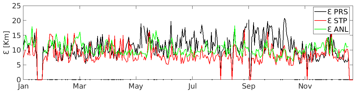
Figure 5Errors of the hourly best analog for the BoB HFR for 2015 (εANL), together with the εSTP and εPRS. The black dots over the timeline show the times when εSTP is higher than εPRS.
The hourly values of εSTP and εPRS have been plotted against their corresponding hourly εANL values for the test year, ordered from minimum to maximum along the x axis, in Fig. 6. We observe that, when εANL is low (less than 13.06 km for this dataset), εSTP is smaller than εPRS. However, as εANL increases, εSTP and εPRS converge until an inflection point beyond which εSTP is slightly greater than εPRS. For the SE BoB experiment, the inflection point occurs at εANL=13.06 km and 88 % of cumulative εANL. Results from the Red Sea HFR system indicate a similar pattern (not shown) when the inflection point occurs at εANL=12.81 km and at 86.4 % of cumulative εANL.
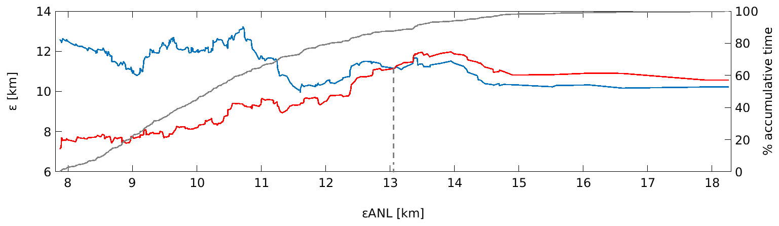
Figure 6The x axis shows the εANL, ordered from minimum to maximum, for the best analog for the test year 2015 for the BoB HFR. The left y axis indicates εSTP (red) and εPRS (blue) for the corresponding εANL. The right y axis indicates the percent of cumulative comparison times, as shown by the gray solid line. The dashed vertical line indicates the crossing point between εSTP and km).
Further analyses to elucidate the mean separation distances (δSTP and δSTP) related to εANL after 6, 12, 24, 36, and 48 h are presented hereinafter. εANL has been plotted together with the mean separation distances of the trajectories (δSTP and δPRS) after 6, 12, 24, 36, and 48 h for each target field (Fig. 7). δSTP is always higher than the δPRS for the 6 h simulation. But the values of δSTP show lower values than δPRS for the lowest εANL for the simulations at 12, 24, 36, and 48 h.

Figure 7The left y axis indicates δSTP (red) and δPRS (blue) for the corresponding εANL after 6, 12, 24, 36, and 48 h. The right y axis is the cumulative percent of time steps in the computation of the mean errors, as indicated by the black line in the plots. The x axis is the εANL, ordered from minimum to maximum, for the best analog for the test year 2015 (BoB HFR system).
The values of the correlation coefficient (R2) between the εANL and δSTP and between εANL and δPRS after 6, 12, 24, 36, and 48 h are summarized in Table 2 in order to analyze the relations between the analog, the L-STP, and the persistence. Values of R2 for εANL and δPRS are small (almost no correlation), varying between 0.01 and 0.11, while correlations between εANL and δSTP are higher, varying between 0.19 and 0.56, and show higher correlation (>0.37) after 12 h of simulations. The behavior of the Red Sea HFR system figures (not shown) is similar to the BoB HFR system.
Table 2Correlation coefficient values between the best εANL and δSTP and between εANL and δPRS after 6, 12, 24, 36, and 48 h of simulation.

Figures 6 and 7 (and the same ones for the Red Sea system, not shown) show that while εANL increases, εSTP and δSTP increase, but εPRS and δPRS decrease, showing an inflexion point (hereinafter εANL(∗)). The εANL(∗) can be calculated just for the historical dataset, but εANL can also be calculated in real time and compared with εANL(∗). It gives a reference value for the forecast skills.
To assess the capabilities of the L-STP methodology, only times when εANL<εANL(∗) are analyzed from now on, as when εANL>εANL(∗) we recommend using persistent currents as a short-term forecast.
3.2 Spatiotemporal performances of the L-STP methodology
Mean separation distances between the truth and forecasted trajectories after different periods of integration times have been computed for both systems just for εANL<εANL(∗) times (Fig. 6) in order to evaluate the temporal forecast capabilities of the methodology. Separation distances computed for the whole test year 2015 are shown in Fig. 8 for the BoB HFR observations.
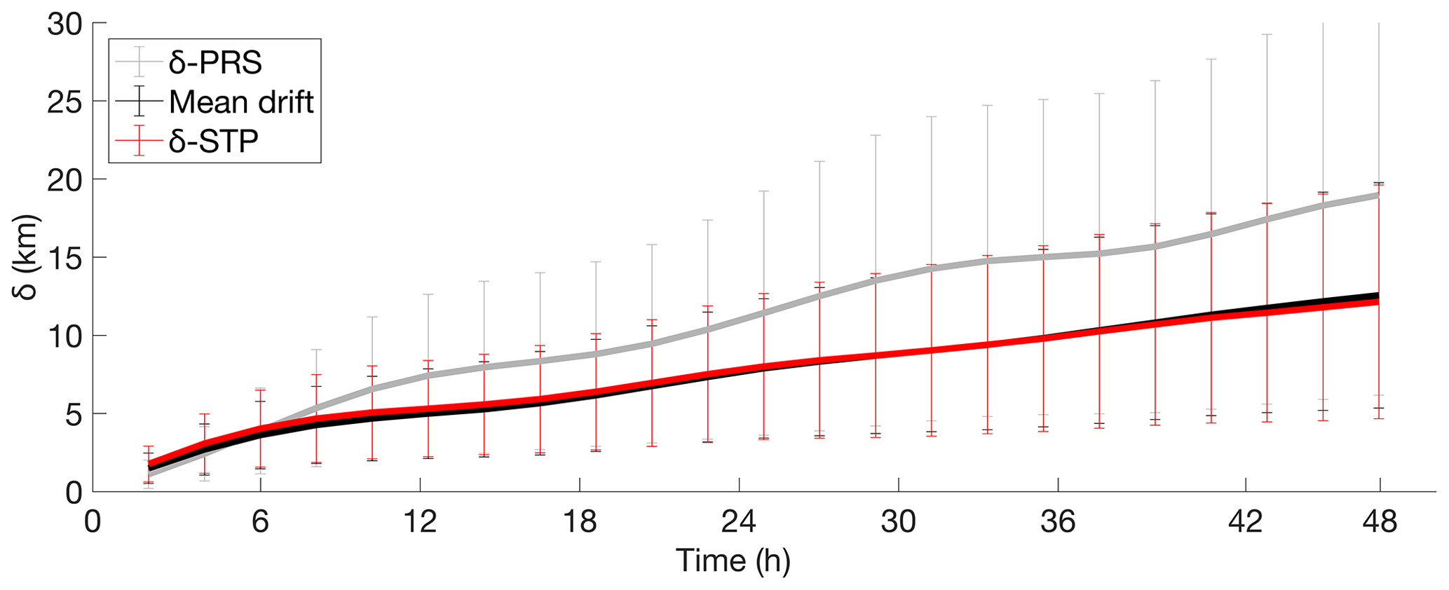
Figure 8Time evolution of the mean separation δSTP and δPRS [km] between the truth and forecast trajectories using the truth and STP–PRS currents and the mean drift with BoB system data for 2015. The mean drift of the truth forecasted trajectories is also computed for each simulation period (the means drift is considered the average of the distances moved by each particle during 48 h).
The separation distances between the measured trajectories and predicted persistent and STP trajectories have similar values during the first 6 h (4 km) of the forecast period, with slightly better results for persistent trajectories. But after 6 h, the separation distance for the forecast based on persistent currents increases faster than using L-STP. At 24 h, the separation distance is 11 km for persistence forecasts and 8 km for L-STP forecasts. The values are 12 and 18 km, respectively, after 48 h of simulation. The mean drift values of the truth trajectories show that the mean drift is similar to the L-STP separation distances during the 48 h.
Temporal mean separation distances between the truth and forecasted trajectories for the central Red Sea HFR system, computed for εANL<εANL(∗), are shown in Fig. 9. The separation distances for the STP forecasts are higher than those forecasts with persistent currents during the first 15 h. After 15 h, the quality of the forecasts reversed and STP produced better results than persistence.
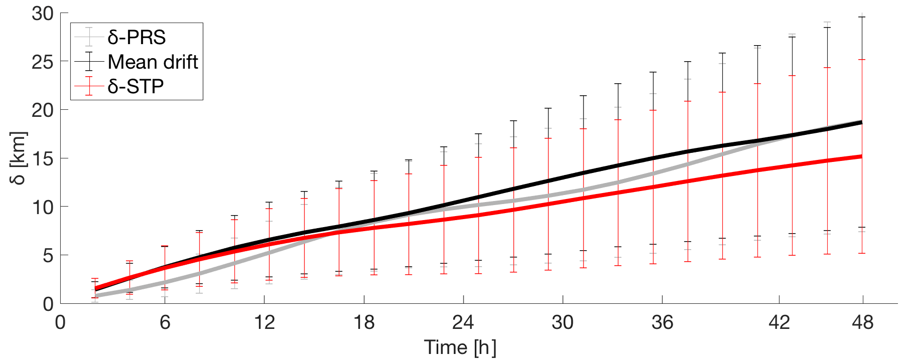
Figure 9Time evolution of the mean separation distances δSTP and δPRS [km] between the real and forecast trajectories using the truth and STP–PRS currents and the mean drift with the Red Sea HFR system data for July 2017 to October 2018. The mean drift of the truth forecasted trajectories is also computed for each simulation period (the means drift is considered the average of the distances moved by each particle during 48 h).
The spatial distributions of the difference between δPRS and δSTP at 6, 12, 24, and 48 h for the BoB and the Red Sea study areas are shown in Figs. 10 and 11.
For the BoB HFR system, the differences are not appreciated during the first 6 h. However, after 12 h of simulation, the advantage of the L-STP is clear in most of the study area, especially outside the continental shelf slope where persistent currents dominate the circulation. The separation values between δPRS and δSTP increase up to 10 km after 48 h of simulation.
For the Red Sea, the significant differences between STP and persistence start after 24 h of simulation and continue until 48 h.
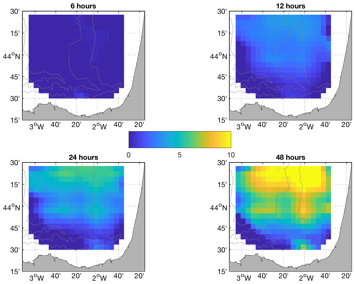
Figure 10Spatial distribution of separation distances [km] between trajectories using L-STP and persistent currents at 6, 12, 24, and 48 h for the BoB HFR system.
In this work, a new methodology to forecast ocean surface currents based on HFR observations has been described. The approach is based on the search of analogs in a trajectory (Lagrangian) space using a previously generated trajectory field catalog. The temporal and spatial skills of the proposed L-STP methodology have been analyzed in the previous section.
The target Lagrangian trajectory maps have been compared with the previously generated trajectory catalog to obtain εANL, εSTP, εPRS, δSTP, and δPRS for each analyzed time. For the BoB system (2015 period), the correlation between εANL and εPRS is 0.05, showing no relation between them, and similar values are obtained for εANL and δPRS (0.01–0.11 from Table 2). The correlation between εANL and εSTP is 0.46, and it varies from 0.19 to 0.56 between εANL and δSTP. Although the correlations between εANL (past) and δSTP or εSTP (future) are low, they suggest that there is a relation between the errors of the analogs and the errors of the L-STP. δSTP is always higher than the δPRS for the 6 h simulation, which means that for the first hour, it is better to use persistence.
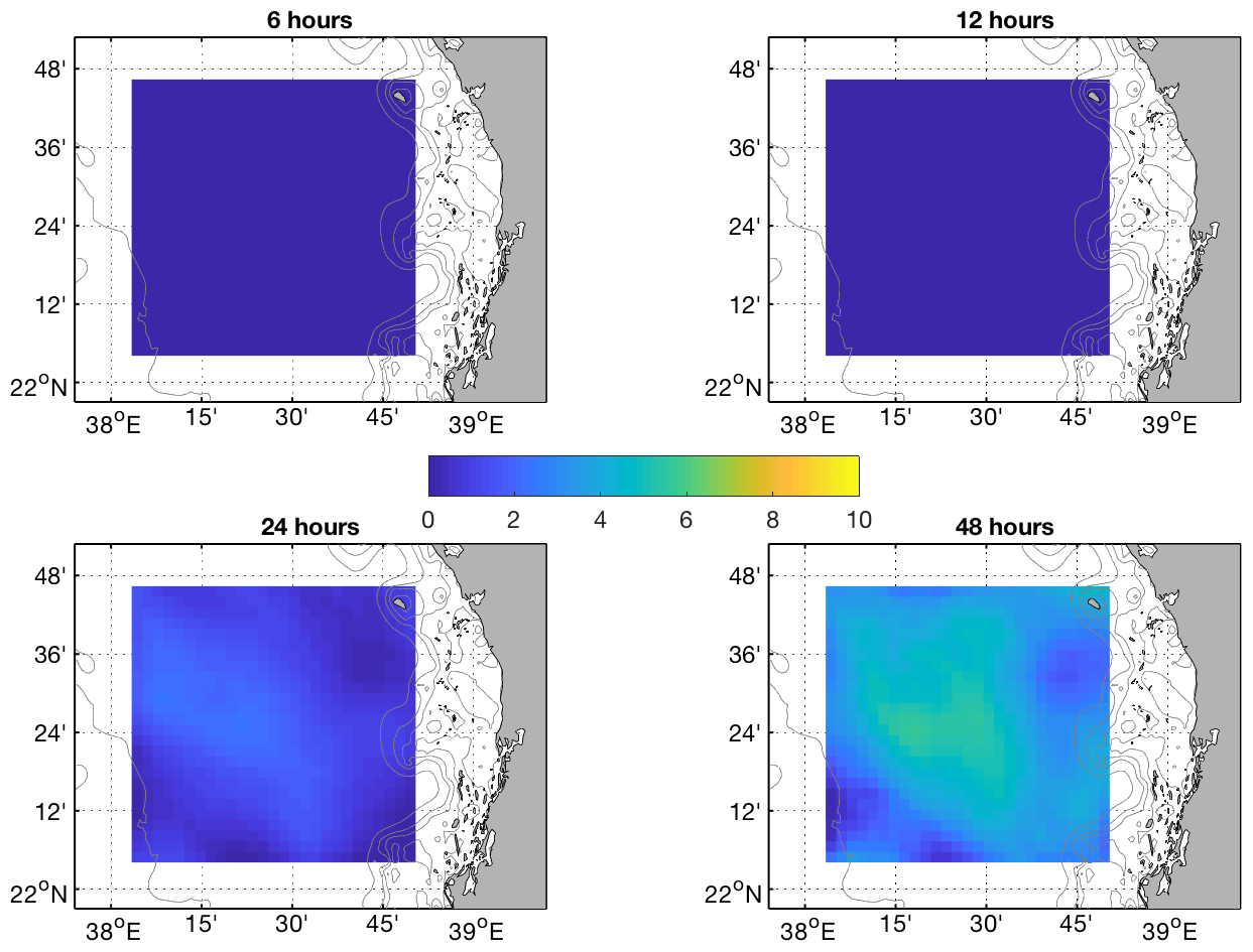
Figure 11Spatial distribution of separation distances [km] between trajectories using L-STP and persistent currents at 6, 12, 24, and 48 h for the Red Sea HFR system.
The εANL(∗) can just be calculated for the historical dataset, but εANL can also be calculated and compared to the previously selected εANL(∗) in real time. It gives a reference value for the forecast skills, and we suggest that εANL can be considered a real-time skill-score metric for the L-STP.
The selection of the best value for εANL(∗) is the main sensitive step of the proposed methodology: the values of εANL are different for each study area and no fixed value can be given. Due to this, an exhaustive analysis of εANL,δSTP, and δPRS of the historical dataset is required to find the correct inflexion point and select a correct εANL(∗), before the method can be applied to a new study area.
Once εANL(∗) is fixed, the skills of the proposed L-STP methodology have been tested in Figs. 8 to 11. The values of the δSTP, compared to previous works in the BoB area, showed that the L-STP produces accurate predictions, which demonstrates the ability of the Lagrangian approach to capture key dynamical features needed to accurately predict the proper dynamical conditions.
For the BoB HFR system, temporal δSTP shows values of 3.5, 5.5, and 8 km after 6, 12, and 24 h, respectively. The δSTP values are similar to the δPRS values during the first 6 h of simulation, but δSTP is lower after that, with 3 and 5.5 km of difference between them after 24 and 48 h of simulation, respectively (Fig. 8). As stated in a previous work, the circulation over the BoB area is dominated by a stable, persistent current field during winter (Solabarrieta et al., 2014), which is reflected by these results in which persistence has good or even slightly better forecasting skill during the first 6 h of forecast than the proposed methodology.
δSTP values for the BoB HFR system are similar to the ones obtained by Solabarrieta et al. (2016) for the whole year, but δSTP values are better for summer months for the same study area. They used the linear autoregressive model, described in Frolov et al. (2012), to forecast HFR current fields, and the errors using that approach were 2.9 and 7.9 km after 6 and 24 h. Although the results obtained in this work only improve the forecast presented in Solabarrieta et al. (2016) during certain periods, the presented methodology has three advantages over the previous method: it is easy to run in real time, it does not require a continuous training period, and it is able to discriminate the times when the usage of the persistence is applicable. On the negative side, it requires the generation of a catalog of past trajectories as the search space for analogs, but once it is ready, it is easily increasable in real time without extra pre-analysis; just add new trajectory fields to the previous catalog.
The values of the δSTP for the Red Sea HFR system follow a similar pattern as the BoB results, with higher separation distances. This may be related to the limited time span of the available dataset, as a better closest analog may be found in a longer dataset.
The spatial comparison of the δSTP and δPRS for the BoB HFR system (Fig. 10) shows that the L-STP has better skills for the entire study area after 12 h of simulations. The skills of the L-STP with respect to the persistence increases with time, showing up to 10 km of improvement relative to persistence at 48 h in some parts of the study area. For the spatial distribution, after 12 h, the smallest differences between δSTP and δPRS occurred over the slope. This is explained by the existence of the persistent seasonal Iberian Poleward Current that flows along the continental slope toward the east along the Spanish coast and northward along the French coast (Solabarrieta et al., 2014). In other words, although the L-STP can be performant in periods of persistent currents, the persistence field can show a better forecast for a short temporal scale (48 h). L-STP will improve those forecasts as soon as spatiotemporal variability increases.
The results for the Red Sea HFR system are similar, but the benefit of the L-STP methodology appears only after 12 h of simulation. Spatially, the improvement is again lower where persistent currents occur, as is the case of the eastern boundary current that flows northward following the eastern Red Sea coastline in the study area (Bower and Farrah, 2015; Sofianos and Johns, 2003; Zarokanellos et al., 2017b). The dominance of the persistent currents is evident in the lower values of the difference between the STP forecasts and the persistence forecasts, as shown in Fig. 11 and in comparison with Fig. 10.
We have compared the capabilities of the L-STP methodology against the forecast based on the persistence of currents. The L-STP method requires long (but not continuous) training periods and improves the results obtained from previously developed HFR forecast systems (Solabarrieta et al., 2016) in the same study area (BoB) for the whole year. However, the L-STP still shows some limitations in predicting some specific dynamical scenarios, i.e., the dynamical conditions created by the persistent IPC (Iberian Poleward Current). We have found that the Lagrangian analog is not able to properly identify such persistence; it performs relatively better during non-persistent periods. Given the fact that persistent events in both study areas are characterized by narrow high-speed jets (i.e., IPC in the BoB), small spatial differences in the location of the main circulation could generate high separation distances between the reference and predicted trajectories. While the trajectory computed from the velocity field predicted from the persistence model is advected in the same jet, the currents obtained from the L-STP are slightly shifted, but just enough to advect the particle in a different position within the jet, therefore generating larger errors (larger εSTP). We have observed that the longer the training period (as in the BoB system), the better the performance of the L-STP method. This suggests that longer training periods would increasing the capability to identify periods of persistent dynamics occurring over the same area, thus improving the performance of the L-STP.
As mentioned, previous efforts to forecast surface currents from HFR data have shown similar results compared with the methodology presented in this paper. However, the advantage of the L-STP method is that it can be used in near-real time with short and non-continuous datasets of around 2–3 years.
A methodology to forecast surface currents with analogs of Lagrangian dynamics in real time has been proposed. This methodology provides accurate forecasts of sea surface currents up to 48 h, and its capability has been tested in terms of spatial and temporal distributions. The methodology has been successfully applied to two distinct coastal regions to evaluate its capabilities in different hydrodynamic regimes, although further analysis using data from more areas is required to generalize the methodology.
Relationships between εANL and εSTP–εPRS suggest that the εANL can be considered a reliable indicator of the method's performance. Taking into consideration all the analyses done in this work, we propose using STP currents for trajectory or velocity field predictions from 12 h forward if the εANL value is lower than εANL(∗). If εANL is higher than εANL(∗) or the forecast is just for the next 6 h, the use of the persistence field is suggested. We also suggest that the εANL(∗) value and forecast transition time need to be carefully evaluated for each study region. This, of course, implies that a minimum dataset is required before the L-STP method can be applied.
Further analysis of analog-finding approaches is required to improve the observed results, especially during periods when currents are persistent. The use of a longer dataset as a training period may improve this aspect. Then, the next step would be to test the methodology for additional periods and other regions to analyze the possibility to find analogs for different sub-regions and to evaluate its functionality in an operational mode.
The methods to find the minimum training period for each system should be analyzed deeper in future works. The minimum training period will be directly related to the variability of the local dynamics, and those should be considered during the analysis.
The HFR_Progs MATLAB package (https://github.com/rowg/hfrprogs, last access: 26 May 2021) has been used to generate total currents from radial files and to fill the spatial gaps in the surface current field using the OMA method, as well as to generate Lagrangian trajectories. The presented forecasting method can therefore be easily implemented as an additional tool to provide short-term forecasts at the same time that they generate total currents.
The data and codes that support the findings of this study are available upon request from the corresponding author, Lohitzune Solabarrieta.
LS worked on the setup of the methodology, data analysis, paper writing, and final submission. IHC worked on the setup of the methodology and the paper writing. AR worked on the setup of the methodology, data analysis, and paper writing. MC worked on the configuration of the methodology and also contributed to the paper writing. GE worked on the configuration of the methodology and also contributed to the paper writing. JM and BHJ contributed to the writing of the paper. AO worked on the configuration of the methodology, data analysis, and the paper writing.
The authors declare that they have no conflict of interest.
This article is part of the special issue “Coastal marine infrastructure in support of monitoring, science, and policy strategies”. It is not associated with a conference.
This work was funded by a Saudi Aramco-KAUST Center for Marine Environmental Observation (SAKMEO) postdoc fellowship to Lohitzune Solabarrieta and by the Integrated Ocean Processes (IOP) group at KAUST. We acknowledge the support of the LIFE-LEMA project (LIFE15 ENV/ES/000252), the European Union's Horizon 2020 research and innovation program under grant agreement nos. 654410 and 871153 (JERICO-NEXT and JERICO-S3 projects), the Directorate of Emergency Attention and Meteorology of the Basque Government, the MINECO/FEDER Project MOCCA (256RTI2018-093941-B-C31), and the Department of Environment, Regional Planning, Agriculture and Fisheries of the Basque Government (Marco Program). This work was partially performed while Alejandro Orfila was a visiting scientist at the Earth, Environmental and Planetary Sciences Department at Brown University through a Ministerio de Ciencia, Innovación y Universidades fellowship (PRX18/00218). Ismael Hernández-Carrasco acknowledges the Vicenç Mut contract funded by the Balearic Island Government and the European Social Fund (ESF) Operational Programme. The HF radar processing toolbox HFR_Progs used to produce OMA was provided by David Kaplan and Michael Cook of the Naval Postgraduate School in Monterey, CA, USA. This is contribution number 1038 of the Marine Research Division of AZTI-BRTA.
This research has been supported by EU Horizon 2020 (grant nos. LIFE15 ENV/ES/000252, 654410, and 871153) and by the Spanish MINECO (grant no. 256RTI2018-093941-B-C31 co-financed with FEDER funds).
This paper was edited by Ingrid Puillat and reviewed by two anonymous referees.
Abascal, A. J., Castanedo, S., Medina, R., Losada, I. J., and Álvarez-Fanjul, E.: Application of HF radar currents to oil spill modelling, Mar. Pollut. Bull., 58, 238–248, 2009.
Abascal A. J., Sanchez, J., Chiri, H., Ferrer, M. I., Cárdenas, M., Gallego, A., Castanedo, S., Medina, R., Alonso-Martirena, A., Berx, B., Turrell, W. R., and Hughes, S. L.: Operational oil spill trajectory modelling using HF radar currents: A northwest European continental shelf case study, Mar. Pollut. Bull., 119, 336–350, https://doi.org/10.1016/j.marpolbul.2017.04.010, 2017.
Abualnaja, Y., Papadopoulos, V. P., Josey, S. A., Hoteit, I., Kontoyiannis, H., and Raitsos, D. E.: Impacts of climate modes on air–sea heat exchange in the Red Sea, J. Clim., 28, 2665–2681, https://doi.org/10.1175/JCLI-D-14-00379.1, 2015.
Barrick, D. E.: Extraction of wave parameters from measured HF radar sea-echo Doppler spectra, Radio Sci., 12, 415–424, https://doi.org/10.1029/RS012i003p00415, 1977.
Barrick, D. E. and Lipa, B. J.: A Compact Transportable HF Radar System for Directional Coastal Wave Field Measurements, in: Ocean Wave Climate, Marine Science, edited by: Earle, M. D. and Malahoff, A., Vol. 8, Springer, Boston, MA, https://doi.org/10.1007/978-1-4684-3399-9_7, 1979.
Barrick, D. E., Fernandez, V., Ferrer, M. I., Whelan, C., and Breivik, Ø.: A short-term predictive system for surface currents from a rapidly deployed coastal HF-Radar network, Ocean Dynam., 62, 725–740, 2012.
Barth, A., Alvera-Azcárate, A., Beckers, J. M., Staneva, J., Stanev, E. V., and Schulz-Stellenfleth, J.: Correcting surface winds by assimilating high-frequency radar surface currents in the German Bight, Ocean Dynam., 61, 599–610, https://doi.org/10.1007/s10236-010-0369-0, 2011.
Bellomo, L., Griffa, A., Cosoli, S., Falco, P., Gerin, R., Iermano, I., Kalampokis, A., Kokkini, Z., Lana, A., Magaldi, M. G., Mamoutos, I., Mantovani, C., Marmain, J., Potiris, E., Sayol, J. M., Barbin, Y., Berta, M., Borghini, M., Bussani, A., Corgnati, L., Dagneaux, Q., Gaggelli, J., Guterman, P., Mallarino, D., Mazzoldi, A., Molcard, A., Orfila, A., Poulain, P. M., Quentin, C., Tintoré, J., Uttieri, M., Vetrano, A, Zambianchi, E., and Zervakis, V.: Toward an integrated HF radar network in the Mediterranean Sea to improve search and rescue and oil spill response: the TOSCA project experience. Toward an integrated HF radar network in the Mediterranean Sea to improve search and rescue and oil spill response: the TOSCA project experience, J. Operat. Oceanogr., 8, 95–107, https://doi.org/10.1080/1755876X.2015.1087184, 2015.
Bower, A. S. and Farrar, J. T.: Air–sea interaction and horizontal circulation in the Red Sea, in: The Red Sea, Springer Earth System Sciences edited by: Rasul, N. M. A. and Stewart, I. C. F., Berlin, Germany, Springer, 329–342, https://doi.org/10.1007/978-3-662-45201-1_19, 2015.
Breivik, Ø. and Saetra, Ø.: Real time assimilation of HF radar currents into a coastal ocean model, J. Mar. Syst., 28, 161–182, https://doi.org/10.1016/S0924-7963(01)00002-1, 2001.
Chao, Y., Li Z., Farrara, K., McWilliams, J.C., Bellingham, J., Capet, X., Chavez, F., Choi, J., Davis, R., Doyle, J., Fratantoni, D. M., Li P., Marchesiello, P., Moline, M. A., Paduan, J., and Ramp, S.: Development, implementation and evaluation of a data-assimilative ocean forecasting system off the central California coast, Deep-Sea Res., 56, 100–126, https://doi.org/10.1016/j.dsr2.2008.08.011, 2009.
Crombie, D. D.: Dopler Spectrum of Sea Echo at 13.56-Mc/s', Nature, 175, 681–682, 1955.
Declerck, A., Delpey, M., Rubio, A., Ferrer, L., Basurko, O. C., Mader, J., and Louzao, M.: Transport of floating marine litter in the coastal area of the south-eastern Bay of Biscay: A Lagrangian approach using modelling and observations, J. Operat. Oceanogr., 12, S111–S125, https://doi.org/10.1080/1755876X.2019.1611708, 2019.
Emery, B. M., Washburn L., and Harlan, J. A.: Evaluating radial current measurements from CODAR high-frequency radars with moored current meters, J. Atmos. Ocean. Tech., 21, 1259–1271, https://doi.org/10.1175/1520-0426(2004)0211259:ERCMFC.2.0.CO;2, 2004.
Esnaola, G., Sáenz, J., Zorita, E., Fontán, A., Valencia, V., and Lazure, P.: Daily scale] wintertime sea surface temperature and IPC-Navidad variability in the southern Bay of Biscay from 1981 to 2010, Ocean Sci., 9, 655–679, https://doi.org/10.5194/os-9-655-2013, 2013.
Frolov, S., Paduan, J., Cook, M., and Bellingham, J.: Improved statistical prediction of surface currents based on historic HF- radar observations, Ocean Dynam., 62, 1111–1122, https://doi.org/10.1007/ s10236-012-0553-5, 2012.
Hammond, T. M., Pattiaratchi, C. B., Osborne, M. J., Nash, L. A., and Collins, M. B.: Ocean surface current radar (OSCR) vector measurements on the inner continental shelf, Cont. Shelf Res., 7, 411–431, https://doi.org/10.1016/0278-4343(87)90108-7, 1987.
Hernández-Carrasco, I., López, C., Hernández-García, E., and Turiel, A.: How reliable are finite-size Lyapunov exponents for the assessment of ocean dynamics?, Ocean Modell., 36, 208–218, 2011.
Hernández-Carrasco, I., Solabarrieta, L., Rubio, A., Esnaola, G., Reyes, E., and Orfila, A.: Impact of HF radar current gap-filling methodologies on the Lagrangian assessment of coastal dynamics, Ocean Sci., 14, 827–847, https://doi.org/10.5194/os-14-827-2018, 2018a.
Hernández-Carrasco, I., Orfila, A., Rossi, V., and Garçon, V.: Effect of small-scale transport processes on phytoplankton distribution in coastal seas, Sci. Rep., 8, 8613, https://doi.org/10.1038/s41598-018-26857-9, 2018b.
Jianping, H., Yuhong, Y., Shaowy, W., and Jifen, C.: An analogue-dynamical long-range numerical weather prediction system incorporating historical evolution, Q. J. R. Meteorol. Soc., 119, 547–565, 1993.
Kaplan, D. M. and Lekien, F.: Spatial interpolation and filtering of surface current data based on open-boundary modal analysis, J. Geophys. Res.-Ocean., 112, c12007, https://doi.org/10.1029/2006JC003984, 2007.
Kohut, J. T. and Glenn, S. M.: Improving HF radar surface current measurements with measured antenna beam patterns, J. Atmos. Ocean. Technol., 20, 1303–1316, 2003.
Lana, A., Marmain, J., Fernández, V., Tintoré, J., and Orfila, A.: Wind influence on surface current variability in the Ibiza Channel from HF Radar, Ocean Dynam., 66, 483–497, https://doi.org/10.1007/s10236-016-0929-z, 2016.
Langodan, S., Cavaleri, L., Vishwanadhapalli, Y., Pomaro, A., Bertotti, L., and Hoteit, I.: Climatology of the Red Sea – Part 1: the wind, Int. J. Climatol., 37, 4509–4517, 2017.
Liu, Y., Weisberg, R. H., and Merz, C. R.: Assessment of CODAR SeaSonde and WERA HF Radars in Mapping Surface Currents on the West Florida Shelf, J. Atmos. Ocean. Technol., 31, 1363–1382, 2014.
Lorenz, E. N.: Atmospheric Predictability as Revealed by Naturally Ocurring Analogues, J. Atmos. Sci., 29, 636–646, 1969.
Manso-Narvarte, I., Caballero, A., Rubio, A., Dufau, C., and Birol, F.: Joint analysis of coastal altimetry and high-frequency (HF) radar data: observability of seasonal and mesoscale ocean dynamics in the Bay of Biscay, Ocean Sci., 14, 1265–1281, https://doi.org/10.5194/os-14-1265-2018, 2018.
Oke, P. R., Allen, J. S., Miller, R. N., Egbert, G. D., and Kosro, P. M.: Assimilation of surface velocity data into a primitive equation coastal ocean model, J. Geophys. Res., 107, 3122, https://doi.org/10.1029/2000JC000511, 2002.
Orfila, A., Molcard, A., Sayol, J. M., Marmain, J., Bellomo, L., Quentin, C., and Barbin, Y.: Empirical Forecasting of HF-Radar Velocity Using Genetic Algorithms, IEEE Trans. Geosci. Remote Sens., 53, 2875–2886, 2015.
Ohlmann, C., White, P., Washburn, L., Emery, B., Terrill, E., and Otero, M.: Interpretation of coastal HF radar–derived surface currents with high- resolution drifter data, J. Atmos. Oceanic Technol., 24, 666–680, 2007.
Paduan, J. D. and Rosenfeld, L. K.: Remotely sensed surface currents in Monterey Bay from shore-based HF radar (coastal ocean dynamics application radar, J. Geophys. Res., 101, 20669–20686, 1996.
Paduan, J. D. and Shulman, I.: HF radar data assimilation in the Monterey Bay area, J. Geophys Res., 109, C07S09, https://doi.org/10.1029/2003JC001949, 2004.
Paduan, J. D. and Washburn, L.: High-Frequency Radar Observations of Ocean Surface Currents, Annu. Rev. Marine. Sci., 5, 115–136, 2013.
Paduan, J. D., Kim, K. C., Cook, M. S., and Chavez, F. P.: Calibration and Validation of Direction-Finding High-Frequency Radar Ocean Surface Current Observations, IEEE J. Ocean. Eng., 31,862–875, https://doi.org/10.1109/JOE.2006.886195, 2006.
Xavier, P. K. and Goswami, B. N.: An Analog Method for Real-Time Forecasting of Summer Monsoon Subseasonal Variability, Mon. Eeather Rev., 135, 4149–4160, https://doi.org/10.1175/2007MWR1854.1, 2007.
Ren, L., Miaro, J., Li, Y., Luo, X., Li, J., and Hartnett, M.: Estimation of Coastal Currents Using a Soft Computing Method: A Case Study in Galway Bay, Ireland, Mar. Sci. Eng., 7, 1–17, https://doi.org/10.3390/jmse7050157, 2019.
Roarty, H., Cook, T., Hazard, L., George, D., Harlan, J., Cosoli, S., Wyatt, L., Alvarez Fanjul, E., Terrill, E., Otero, M., Largier, J., Glenn, S., Ebuchi, N., Whitehouse, B., Bartlett, K., Mader, J., Rubio, A., Corgnati, L., Mantovani, C., Griffa, A., Reyes, E., Lorente, P., Flores-Vidal, X., Saavedra-Matta, K. J., Rogowski, P., Prukpitikul, S., Lee, S. H., Lai, J. W., Guerin, C. A., Sanchez, J., Hansen, B., and Grilli, S.: The Global High Frequency Radar Network, Front. Mar. Sci., 6, 164, https://doi.org/10.3389/fmars.2019.00164, 2019.
Rubio, A., Fontán, A., Lazure, P., González, M., Valencia, V., Ferrer, L., Mader, J., and Hernández, C.: Seasonal to tidal variability of currents and temperature in waters of the continental slope, southeastern Bay of Biscay, J. Mar. Syst., 109/110, S121–S133, https://doi.org/10.1016/j.jmarsys.2012.01.004, 2013a.
Rubio, A., Solabarrieta, L., González, M., Mader, J., Castanedo, S., Medina, R., Charria, G., and Aranda, J.: Surface circulation and Lagrangian transport in the SE Bay of Biscay from HF radar data, MTS/IEEE OCEANS—Bergen, 2013, IEEE, 7 pp., https://doi.org/10.1109/OCEANS-Bergen.2013.6608039, 2013b.
Rubio, A., Mader, J., Corgnati, L., Mantovani, C., Griffa, A., Novellino, A., Quentin, C., Wyatt, L., Schulz-Stellenfleth, J., Horstmann, J., Lorente, P., Zambianchi, E., Hartnett, M., Fernandes, C., Zervakis, V., Gorringe, P., Melet, A., and Puillat, I.: HF radar activity in European coastal seas: next steps towards a pan-European HF radar network, Front. Mar. Sci., 4, 8, https://doi.org/10.3389/fmars.2017.00008, 2017.
Rubio, A., Caballero, A., Orfila, A., Hernández-Carrasco, I., Ferrer, L., González, M., Solabarrieta, L., and Mader, J.: Eddy-induced cross-shelf export of high Chl-a coastal waters in the SE Bay of Biscay, Remote Sens. Environ., 205, 290–304, 2018.
Rubio, A., Manso-Narvarte, I., Caballero, A., Corgnati, L., Mantovani, C., Reyes, E., Griffa, A., and Mader, J.: The seasonal intensification of the slope iberian poleward current, copernicus marine service ocean state report, J. Oper. Oceanogr., 12, 13–18, https://doi.org/10.1080/1755876X.2019.1633075, 2019.
Rubio, A., Hernández-Carrasco, I., Orfila, A., González, M., Reyes, E., Corgnati, L., Berta, M., Griffa, A., and Mader, J.: A lagrangian approach to monitor local particle retention conditions in coastal areas. copernicus marine service ocean state report, J. Oper. Oceanogr., 13, 1785097, https://doi.org/10.1080/1755876X.2020.1785097, 2020.
Sayol, J. M., Orfila, A., Simarro, G., Conti, G., Renault, L., and Molcard, A.: A Lagrangian model for tracking surface spills and SaR operations in the ocean, Env. Mod. Softw., 52, 74–82, https://doi.org/10.1016/j.envsoft.2013.10.013, 2014.
Schmidt, R.: Multiple emitter location and signal parameter estimation, IEEE Trans. Antennas Propag., 34, 276–280, https://doi.org/10.1109/TAP.1986.1143830, 1986.
Schott F., Frisch, A. S., Leaman, K., Samuels, G., and Popa Fotino, I.: High-Frequency Doppler Radar Measurementsof the Florida Current in Summer 1983, J. Geophys. Res., 90, 9006–9016, 1985.
Shao, Q. and Li, M.: An improved statistical analogue downscaling procedure for seasonal precipitation forecast, Stoch. Environ. Res. Risk Assess., 27, 819–830, https://doi.org/10.1007/s00477-012-0610-0, 2013.
Sofianos, S. S. and Johns, W. E.: An oceanic general circulation model (OGCM) investigation of the Red Sea circulation: 2. Three-dimensional circulation in the Red Sea, J. Geophys. Res., 108, 3066, https://doi.org/10.1029/2001jc001185, 2003.
Solabarrieta, L., Rubio, A., Castanedo, S., Medina, R., Charria, G., and Hernández, C.: Surface water circulation patterns in the southeastern Bay of Biscay: new evidences from HF radar data, Cont. Shelf Res., 74, 60–76, https://doi.org/10.1016/j.csr.2013.11.022, 2014.
Solabarrieta, L., Rubio, A., Cárdenas, M., Castanedo, S., Esnaola, G., Méndez, F. J., Medina, R., and Ferrer, L.: Probabilistic relationships be- tween wind and surface water circulation patterns in the SE Bay of Biscay, Ocean Dynam., 65, 1289–1303, https://doi.org/10.1007/s10236-015-0871-5, 2015.
Solabarrieta, L., Frolov, S., Cook, M., Paduan, J., Rubio, A., González, M., Mader, J., and Charria, G.: Skill Assessment of HF Radar–Derived Products for Lagrangian Simulations in the Bay of Biscay, J. Atmos. Ocean. Technol., 33, 2585–2597, https://doi.org/10.1175/JTECH-D-16-0045.1, 2016.
Stanev, E. V., Schulz-Stellenfleth, J., Staneva, J., Grayek, S., Seemann, J., and Petersen, W.: Coastal observing and forecasting system for the German Bight – estimas of hydrophysical states, Ocean Sci., 7, 569–583, https://doi.org/10.5194/os-7-569-2011, 2011.
Ullman, D. S., O'Donnell, J., Kohut, J., Fake, T., and Allen, A.: Trajectory prediction using HF radar surface currents: Monte Carlo simulations of prediction uncertainties, J. Geophys. Res., 111, C12005, https://doi.org/10.1029/2006JC003715, 2006.
Vilibicì, I., Šepicì, J., Mihanovicì, H., Kalinicì, H., Cosoli, S., Janekovicì, I., Žagar, N., Jesenko, B., Tudor, M., Dadicì, V., and Ivankovicì, D.: Self-organizing maps-based ocean currents forecasting system, Sci. Rep., 6, 22924, https://doi.org/10.1038srep22924, 2016.
Yao, F., Hoteit, I., Pratt, L. J., Bower, A. S., Zhai, P., Kohl, A., and Gopalakrishnan, G.: Seasonal overturning circulation in the Red Sea: 1. Model validation and summer circulation, J. Geophys. Res.-Ocean., 119, 2238–2262, https://doi.org/10.1002/2013JC009004, 2014a.
Yao, F., Hoteit, I., Pratt, L. J., Bower, A. S., Kohl, A., Gopalakrishnan, G., and Rivas, D.: Seasonal overturning circulation in the Red Sea: 2. Winter circulation, J. Geophys. Res.-Ocean., 119, 2263–2289, https://doi.org/10.1002/2013JC009331, 2014b.
Zarokanellos, N. D., Kürten, B., Churchill, J. H., Roder, C., Voolstra, C. R., Abualnaja, Y., and Jones, B. H.: Physical mechanisms routing nutrients in the central Red Sea, J. Geophys. Res.-Ocean., 122, 9032–9046, https://doi.org/10.1002/2017JC013017, 2017a.
Zarokanellos, N. D., Papadopoulos, V. P., Sofianos, S. S., and Jones, B. H.: Physical and biological characteristics of the winter-summer transition in the Central Red Sea, J. Geophys. Res.-Ocean., 122, 6355–6370, https://doi.org/10.1002/2017JC012882, 2017b.
Zhan, P., Subramanian, A. C., Yao, F., and Hoteit, I.: Eddies in the Red Sea: A statistical and dynamical study, J. Geophys. Res.-Ocean., 119, 3909–3925, https://doi.org/10.1002/2013JC009563, 2014.
Zelenke, B. C.: An Empirical Statistical Model Relating Winds and Ocean Surface Currents, Master of Science in Oceanography – Thesis, Oregon State University, Oregon State University Publisher, Corvallis, Oregon, 2005.