the Creative Commons Attribution 4.0 License.
the Creative Commons Attribution 4.0 License.
 | 06 May 2021
The mesoscale eddy field in the Lofoten Basin from high-resolution Lagrangian simulations
Johannes S. Dugstad
Pål Erik Isachsen
Ilker Fer
Warm Atlantic-origin waters are modified in the Lofoten Basin in the Nordic Seas on their way toward the Arctic. An energetic eddy field redistributes these waters in the basin. Retained for extended periods, the warm waters result in large surface heat losses to the atmosphere and have an impact on fisheries and regional climate. Here, we describe the eddy field in the Lofoten Basin by analyzing Lagrangian simulations forced by a high-resolution numerical model. We obtain trajectories of particles seeded at three levels – near the surface, at 200 m and at 500 m depth – using 2D and 3D velocity fields. About 200 000 particle trajectories are analyzed from each level and each simulation. Using multivariate wavelet ridge analysis, we identify coherent cyclonic and anticyclonic vortices in the trajectories and describe their characteristics. We then compare the evolution of water properties inside cyclones and anticyclones as well as in the ambient flow outside vortices. As measured from Lagrangian particles, anticyclones have longer lifetimes than cyclones (16–24 d compared to 13–19 d), a larger radius (20–22 km compared to 17–19 km) and a more circular shape (ellipse linearity of 0.45–0.50 compared to 0.51–0.57). The angular frequencies for cyclones and anticyclones have similar magnitudes (absolute values of about 0.05f). The anticyclones are characterized by warm temperature anomalies, whereas cyclones are colder than the background state. Along their path, water parcels in anticyclones cool at a rate of 0.02–0.04 , while those in cyclones warm at a rate of 0.01–0.02 . Water parcels experience a net downward motion in anticyclones and upward motion in cyclones, often found to be related to changes in temperature and density. The along-path changes in temperature, density and depth are smaller for particles in the ambient flow. An analysis of the net temperature and vorticity fluxes into the Lofoten Basin shows that while vortices contribute significantly to the heat and vorticity budgets, they only cover a small fraction of the domain area (about 6 %). The ambient flow, including filaments and other non-coherent variability undetected by the ridge analysis, hence plays a major role in closing the budgets of the basin.
- Article
(17121 KB) - Full-text XML
- BibTeX
- EndNote


The Lofoten Basin (LB) in the Norwegian Sea is an important region for the retention and modification of the warm Atlantic Water (AW) as it flows northward towards the Arctic Ocean (Mauritzen, 1996; Rossby et al., 2009b; Koszalka et al., 2011). In this region, the AW splits into two branches (Poulain et al., 1996; Orvik and Niiler, 2002) (Fig. 1a): the Norwegian Atlantic Slope Current (Slope Current hereinafter) and the Norwegian Atlantic Front Current (Front Current hereinafter). These currents enclose the LB in the east along the continental slope off Norway and in the west along the Mohn Ridge, respectively. The warm AW spreads into the basin between these two branches. The LB is therefore a major heat reservoir in the Nordic Seas (Nilsen and Falck, 2006), and its heat content has increased over the last 3 decades (Broomé et al., 2020). Exposed to increased residence times, winter cooling and vertical mixing, the AW layer in the basin thickens and can reach depths of 500 m (Mauritzen, 1996; Bosse et al., 2018).
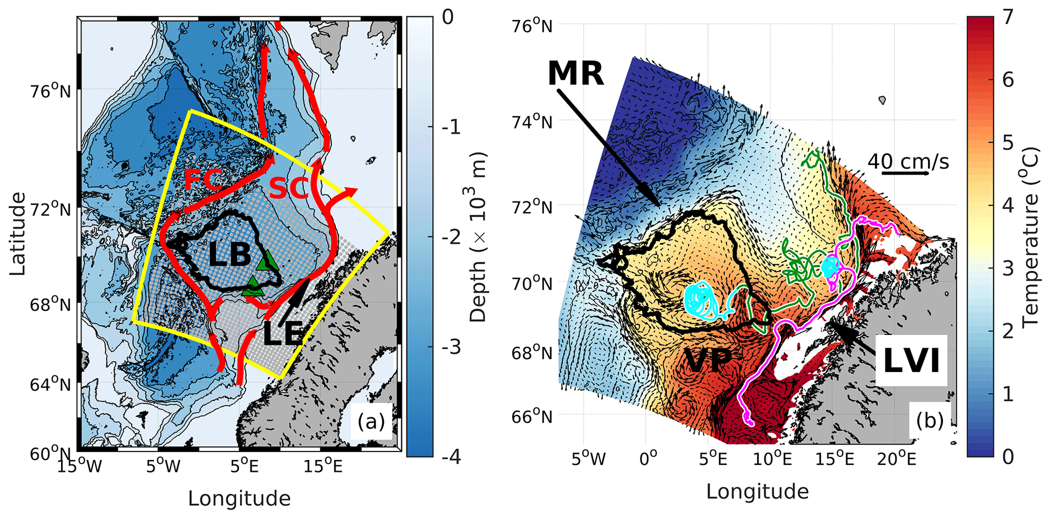
Figure 1(a) Bathymetry of the Nordic Seas together with the main pathways of the Atlantic Water (red), the ROMS model domain (yellow) used for the OpenDrift simulations, and the deployment grid of the drifters (gray dots). Highlighted black contour shows the LB approximated by the 3000 m isobath with green triangles marking the edges of the southeastern part (see Sect. 4.3). (b) A zoom on the model domain showing the Eulerian mean temperature (color bar) and the mean velocity (arrows, scale on the upper right) at 200 m depth, time averaged between 1996 and 2000. A couple of 2D trajectories at 200 m are superimposed (green and magenta), with the ridge segments marked in cyan. Abbreviations are as follows: LB – Lofoten Basin; LE – Lofoten Escarpment; FC – Front Current; SC – Slope Current; MR – Mohn Ridge; VP – Vøring Plateau; LVI – Lofoten–Vesterålen islands.
Both the Slope Current and the LB (here defined as the central basin enclosed by the 3000 m isobath, highlighted by the black contour in Fig. 1) are characterized by energetic eddy fields. The Slope Current, in particular, is favorable for baroclinic instability as it passes very steep topography off the Lofoten–Vesterålen islands (Köhl, 2007; Isachsen, 2015; Fer et al., 2020). This results in enhanced eddy kinetic energy (EKE) levels (Andersson et al., 2011; Koszalka et al., 2011; Volkov et al., 2015; Fer et al., 2020) and large lateral diffusion rates (Koszalka et al., 2011). The EKE field in the LB is particularly strong towards the center of the basin. There, at a mean position of around 70∘ N, 3∘ E, the Lofoten Basin Eddy (LBE, also referred to as the Lofoten Vortex) (Ivanov and Korablev, 1995; Köhl, 2007; Raj et al., 2015; Fer et al., 2018) appears as a permanent anticyclone with a relative vorticity between −0.7f (Fer et al., 2018) and −f (Søiland and Rossby, 2013), where f is the Coriolis frequency. A secondary EKE maximum is observed towards the southeastern boundary of the 3000 m isobath surrounding the basin.
The vigorous eddy field is thought to have an impact on the thickening of the AW layer in the LB and towards the slope. For example, studies of regional hydrographic observations (Rossby et al., 2009b; Bosse et al., 2018) have shown that isopycnals that define the AW layer reach the deepest levels in the LBE and in the secondary EKE maximum. The deep-reaching AW is particularly studied in the LBE and has been related to a vertical stacking of lighter anticyclones that interact with the LBE and push the AW in the LBE further down (Trodahl et al., 2020). In addition, the LBE as well as other energetic eddies are hypothesized to enhance small-scale turbulence, thereby mixing AW to deeper levels and also causing irreversible changes to the AW properties (Volkov et al., 2015; Bosse et al., 2018). While regionally integrated transformation of AW can be estimated from hydrographic data sets, property changes in water parcels along their trajectories, as well as the role of mesoscale eddies versus other flow features along the trajectories, remain largely unknown.
The exchange of AW with the LB (AW–LB exchange) has also been studied extensively. Earlier literature has suggested that much of the warm AW in the LB stems from anticyclonic eddies in the form of long-lived coherent vortices that shed off from the Slope Current and then bring with them heat and vorticity westward into the basin (Köhl, 2007; Isachsen et al., 2012; Volkov et al., 2013; Raj et al., 2016). However, how far these vortices are advected and how often they reach deep into the LB is uncertain. Raj et al. (2016) used satellite altimetry to estimate that about 75 % of cyclonic and anticyclonic vortices in the region have a lifetime shorter than 30 d and that their drift speed never exceeds 8.3 cm s−1. To cover a typical distance from the slope to the center of the basin within a lifetime of 30 d, an eddy translation speed of 16 cm s−1 is required, which exceeds the upper value found by Raj et al. (2016). This suggests that other processes may have to contribute significantly to the AW–LB exchange. Indeed, previous Lagrangian studies (Koszalka et al., 2011; Dugstad et al., 2019a, b) have shown that surface drifters carried in a broad slab of water in the southern sector of the basin interact with the LB. And a Eulerian analysis by Dugstad et al. (2019a) showed that a key surface inflow contribution to the LB heat budget is primarily related to the mean-flow component.
To describe and quantify the role of the eddy field for the AW–LB exchanges, it is important to note that energetic vortices not only carry around the properties trapped in their cores but also stir and transport more passive water masses surrounding them. In an idealized simulation of an unstable eastern boundary current over steep topography with a deeper basin to the west (mimicking the domain we study here), Spall (2010) identified narrow structures or “filaments” surrounding anticyclonic eddies that can carry large cyclonic vorticity and hence make an important contribution to the net vorticity flux to the basin. It seems plausible that transport of such filaments is important to the heat and vorticity budgets also of the real Lofoten Basin, but to our knowledge a quantification of this has not been done before.
In this work we study the eddy field around the LB from a Lagrangian perspective. We perform Lagrangian simulations forced by high-resolution model outputs and extract eddy signals from synthetic particle trajectories using the method of multivariate wavelet ridge analysis (Lilly and Olhede, 2009; Lilly et al., 2011). We will thus distinguish between eddies and the ambient flow. By “eddies” we will be referring to coherent vortices in which trapped particles undergo repeated orbits, or oscillations, within a range of time and space scales. The “ambient flow” will then refer to all features other than the coherent vortices, including large-scale mean flows, filaments and other smaller-scale non-coherent flow features. The study consists of three main parts: (1) a quantification of the eddies and their characteristics (shape, size, rotation speed, spatial distribution), (2) a comparison of how the characteristics of water masses in eddies and the ambient flow evolve with time, and (3) calculations of the net temperature and vorticity fluxes into the LB with an assessment of the relative contribution from eddies and the ambient flow.
2.1 Ocean model
The Lagrangian trajectories are integrated by using output from a high-resolution Regional Ocean Modelling System (ROMS) configuration in the Nordic Seas. ROMS is a hydrostatic model solving the primitive equations on a staggered C grid with terrain-following vertical coordinates (Haidvogel et al., 2008; Shchepetkin and McWilliams, 2009). We use a fourth-order centered scheme for vertical advection and a third-order upwind scheme for horizontal tracer and momentum advection. No explicit horizontal eddy viscosity or diffusion is applied, but the upwind advection scheme exhibits implicit numerical diffusion. Vertical mixing processes that are not resolved by the model grid are parametrized by the k−ϵ version of the general length scale scheme (Umlauf and Burchard, 2003; Warner et al., 2005). The open lateral boundaries are relaxed toward monthly fields from the Global Forecast Ocean Assimilation Model (MacLachlan et al., 2015) and the atmospheric forcing is provided by 6-hourly fields from the ERA-Interim atmospheric reanalysis (Dee et al., 2011). The model has an 800 m horizontal grid resolution and 60 vertical layers. The vertical resolution is 2–5 m near the surface and 60–70 m towards the bottom. Model outputs are stored every 6 h between January 1996 and January 2000. This spatial and temporal resolution allows the model to resolve mesoscale and to some extent also submesoscale features (Isachsen, 2015; Trodahl and Isachsen, 2018).
2.2 Lagrangian simulations
The Lagrangian simulations are the same as in Dugstad et al. (2019b). We use OpenDrift (Dagestad et al., 2018), an open source Python-based framework for Lagrangian modeling which operates offline by using the stored model velocity output. We perform two experiments: one using only the horizontal velocity (2D experiment) and a second one using the full three-dimensional velocity field (3D experiment). The Lagrangian positions (longitude, latitude, depth) are updated using the 6-hourly model currents by applying a fourth-order Runge–Kutta integration routine and are stored at 6 h intervals. Potential temperature, salinity and velocity fields are linearly interpolated onto the particles. We also create daily fields of relative vorticity and the Okubo–Weiss parameter (see Sect. 3.1) and interpolate these similarly. We do not add explicit lateral or vertical diffusion to the drifters. The ocean model is very high resolution, and a comparison between synthetic 2D trajectories and real 2D surface drifters has shown that lateral relative dispersion is well reproduced (Dugstad et al., 2019b). We considered whether the omission of vertical diffusion might lead to a misleading representation of the vertical motion of the particles. However, if adding vertical diffusion, the tuning of such diffusion (implemented as a random walk) is a fairly complex endeavor and is often omitted for such high-resolution modeling (Gelderloos et al., 2017; Dugstad et al., 2019b; Wagner et al., 2019). We essentially believe that adding vertical diffusion would lead to a larger spread of the particles in the vertical but would not significantly affect the systematic behavior of the vertical motion of the flow. We return to this issue in the conclusion section.
In all simulations we deploy particles at three levels (15, 200 and 500 m) in sets of 1600 particles every week for 3 years, from 1 January 1996 to 1 January 1999, with about 20 km spacing between particles (deployment positions are shown in Fig. 1a). In total, this gives 156 weeks of deployments and particles at each deployment depth. The particles are given a lifetime of 1 year, i.e., the trajectory data end on 1 January 2000. We remove all particles that are deployed in areas shallower than 200 m. After excluding these, the number of particles is reduced to 225 000 at 15 and 200 m and 195 000 at 500 m for both the 2D and 3D simulation. The spacing and temporal seeding frequency of the particles is designed to achieve relatively uncorrelated motions between different particles, thereby giving independent statistics when we trace and describe the characteristics of eddies and other flow features. With this spacing and temporal seeding frequency, an eddy with an average radius of 20 km and an average lifetime of 1 month will typically be sampled by 20–25 particles directly deployed in the eddy in addition to the particles that might enter the eddy from outside. For simplicity, we will refer to the Lagrangian particles as “drifters” and use “temperature” and “density” for potential temperature and potential density.
2.3 Multivariate wavelet ridge analysis
To identify long-lived coherent vortices in the Lagrangian trajectories, we perform a multivariate wavelet ridge analysis (MWRA), which has been developed for the purpose of finding “loops” in drifter trajectories and hence identifying whether the drifters are inside coherent vortices. We describe the basic concepts of the method here, but more details can be found in Lilly and Olhede (2009) and in Lilly et al. (2011).
A drifter deployed in position (xo,yo) that moves around with time will experience east–west, x(t), and north–south, y(t), displacements relative to the deployment position. The vector time series thus represents the displacement signal for the drifter, relative to the deployment position. Loops in a drifter trajectory would occur as an oscillating signal in the time series z(t). The MWRA routine seeks to trace this oscillation by performing a wavelet transformation of z(t):
where wz,ψ is the wavelet transform, ψ is the wavelet used with the asterisk denoting the complex conjugate, s is a scaling factor that controls the contraction or dilation of the wavelet in time, τ is the time which we integrate over, and t is the shift as the wavelet is shifted in time along z. The wavelet transform wz,ψ can be regarded as a projection of the time series z onto the wavelet ψ for different choices of t and s. Hence, large values of wz,ψ are expected where the projection of z onto ψ is good, that is in regions where z experiences oscillations similar to the oscillations given by ψ for a given t and s. In other words, given the right conditions on t and s, when a looping drifter trajectory leads to oscillations in z, this will result in large values of wz,ψ.
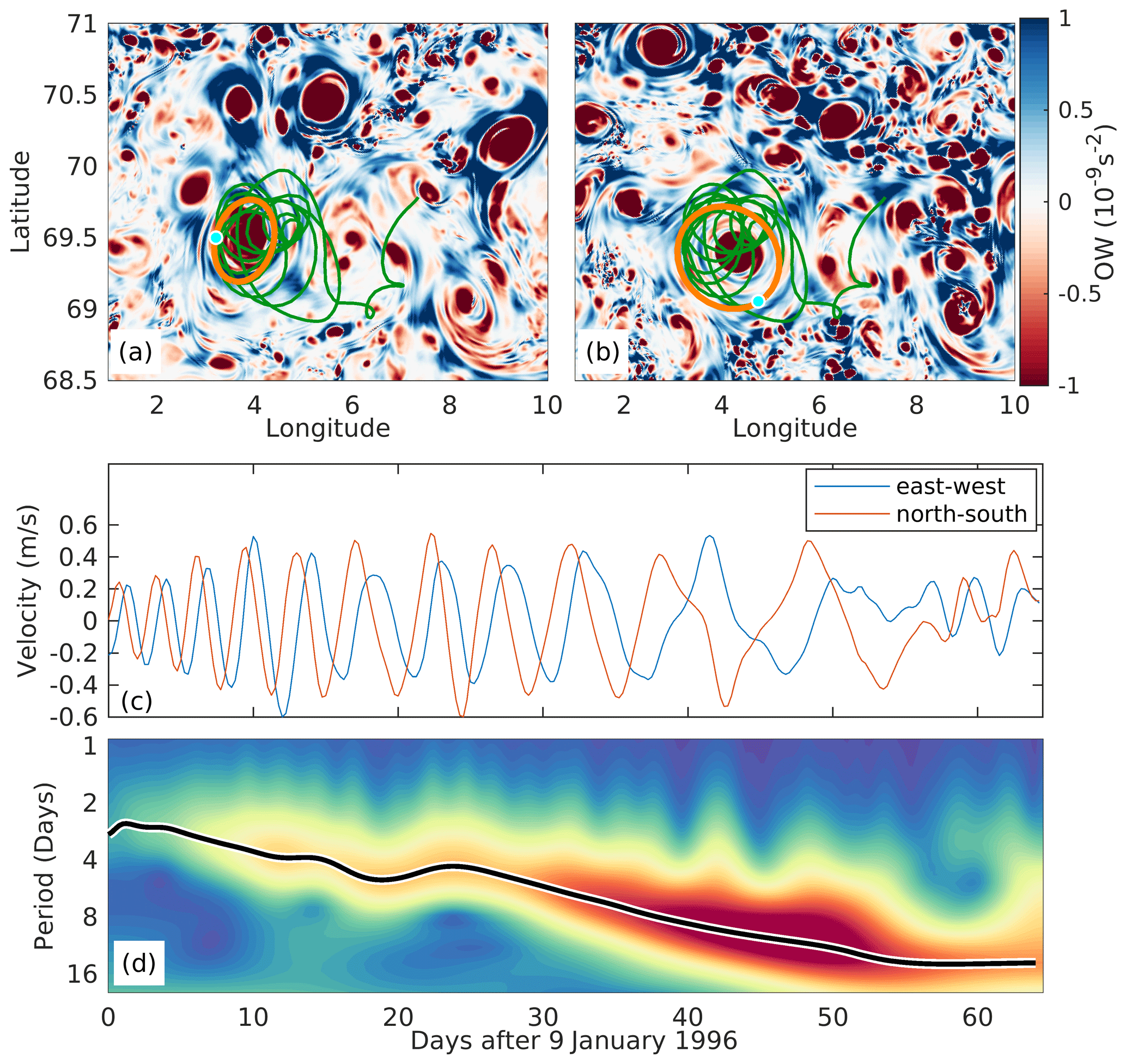
Figure 2(a, b) The basin trajectory (the ridge segment) from Fig. 1b superimposed on snapshots of the OW field (see text) from (a) 1 February 1996 and (b) 15 February 1996. Cyan dots and orange ellipses show the position of the drifter and the instantaneous spanned-out ellipse (see text) as computed from the MWRA routine at the two dates. Color bar unit is 10−9 s−2. Example of the MWRA routine applied to the trajectory is shown in (c, d). (c) The east–west and north–south velocities (u and v) of the trajectory. (d) The magnitude of the total wavelet transform , where and are the absolute values of the positive and negative rotary transforms, respectively. The black line indicates the ridge which is given by the maximum of .
The MWRA routine looks for “ridge points”. A ridge point is defined as a point on the t–s plane that satisfies
meaning that ridge points are locations where the norm of the wavelet transform vector experiences a local maximum with respect to the scale s. Persistent oscillations in z with time will thereby lead to a continuous curve of adjacent ridge points in time that are connected to each other. We refer to this curve as a “ridge”. Per definition, the ridge traces out the signals with the largest intensity/energy in the wavelet transform. Therefore, when a drifter contains a ridge, this is interpreted as indicating that the drifter is caught inside an eddy, given our parameter choices (see below). For more details, see Lilly et al. (2011).
After identifying the ridges, the MWRA routine outputs the longitudes and latitudes of each ridge. At a given position and time along a ridge, the curve traced out by its instantaneous motion can be described as an ellipse with major axis a and minor axis b. We also obtain such ellipse parameters at each instantaneous position on a ridge (every ridge point) to identify the typical characteristics of the eddy (size, shape, rotation speed, etc.). Finally, “residual” longitudes and latitudes, that is longitudes and latitudes along the ridge after subtracting the oscillating eddy signal, are also computed to represent the location of the mass center of the eddy tracked by the drifter. A summary of the drifter variables used in this study is given in Table 1.
An example of the MWRA routine applied to the ridge (cyan) of the green trajectory in Fig. 1 is given in Fig. 2. This drifter was deployed close to the center of the LBE on 8 January 1996 and immediately started to loop around, leading to the detection of a ridge from 9 January to 14 March 1996. The ridge plotted over snapshots of the Okubo–Weiss field (described in Sect. 3.1) shows that the drifter loops around the LBE (shown by negative/red values/colors). The east–west (u) and north–south (v) velocities (Fig. 2c) show longer oscillation periods with time, suggesting that the drifter loops with a larger radius as time advances. The magnitude of the total wavelet transform (Fig. 2d) shows a persistent region of high intensity indicating adjacent ridge points. Thus, the maximum of traces out a well-defined ridge (black curve) which indeed confirms an oscillation period that increases with time. Note here that we have not included a “cone of influence” to indicate the validity range of the wavelet transform. The MWRA routine performs trimming to the ridges, meaning the edges that may be caused by spin-up effects are removed. The ridges are therefore within the valid regime of the wavelet transform. This is also the reason why the ridge is detected on 9 January although the drifter was deployed in the LBE on 8 January. This is a general feature: due to the ridge trimming, the MWRA routine will never identify ridges on the day of the drifter deployment. The ellipse parameters (Table 1) are obtained by analyzing the instantaneous motion of the drifter along the ridge to estimate the size, shape, rotation speed, etc., of the eddy. Two exemplary ellipses are plotted for 1 February 1996 and 15 February 1996 (orange ellipses in Fig. 2a and b, respectively). The size of the ellipses increase with time, again indicating that the drifter loops with a larger radius with time.
Table 1List of output from the MWRA routine. In descriptions, a and b are the semi-major axis and the semi-minor axis of an ellipse.
For each drifter the MWRA routine may find zero, one or several separate ridges, each one given with indices along the drifter trajectories. This means that for a given drifter trajectory, we are able to identify where and when the drifter experiences ridges. By applying the routine to a large number of drifter trajectories, we can describe the eddy characteristics and behavior using statistics. Furthermore, since we also track the drifters before and after they experienced ridges, we can compare the eddy characteristics and behavior with that of the ambient flow outside eddies.
To objectively select ridges that are associated with eddies, some choices are made. Before running the MWRA routine, we choose a frequency band of (i.e., we only allow oscillations in z(τ) within this frequency band), similar to Lilly et al. (2011), where the non-dimensional frequency is the ratio of the angular frequency ω of the vortex/eddy as sampled by drifters and the local Coriolis frequency f. The lower limit allows us to capture oscillations far out on an eddy flank, while the upper limit is sufficient to capture the nonlinear mesoscale features in the region. Note that , in solid body rotation, equals half of the Rossby number , where ζ is the vertical component of relative vorticity. Nonlinear features, such as the LBE having –1, would therefore be captured by this band. In fact, never exceeds 0.52, meaning that choosing a frequency band of would not change our results. An important choice is the minimum ridge length threshold. We assign the ridge length both in terms of time (how long the drifters experience a ridge) and in terms of the number of cycles the drifters experience along the ridge.
This second threshold is chosen as a function of the number of oscillations within the wavelet we use, leading to the problem of first choosing wavelet duration , where β and γ are constants controlling the form of the wavelet (Lilly and Olhede, 2012). The wavelet duration is defined such that is approximately the number of oscillations contained within the wavelet in the time domain (Lilly and Olhede, 2009) and the number of oscillations is controlled by the parameters β and γ. We follow Lilly and Olhede (2012) and Lilly et al. (2011), who state that a good choice would be the so-called “Airy” wavelet giving a wavelet duration of . This value gives a high degree of time concentration at some expense of the frequency resolution but captures the features we are looking for. To accurately identify eddies in our ridges, we set the ridge length (in terms of cycles) to . This is a rather strict threshold and twice as large as the value set in Lilly et al. (2011). However, they find that ridges with fewer or the same amount of cycles as their set threshold (1.6) are usually spurious because one looks for ridges with fewer cycles than the wavelet itself. The ridges become statistically more significant by increasing the threshold.
In terms of time, we choose a minimum ridge length of 2 d. However, due to the choice of ridge length in terms of cycles, this latter choice did not affect the results. Lastly, through the ridge trimming (mentioned above in this section) we also remove about oscillations from each end of a ridge (Lilly et al., 2011). As a result, the ridges can have a minimum of 1.6 cycles. We further discuss the ridge length in Sects. 3.1 and 4.1.

Figure 3Distribution of ridge points in the radius–orbital velocity () plane for 3D drifters deployed at 200 m. Positive and negative velocities correspond to cyclonic and anticyclonic motions, respectively. Colors mark (a) log10 of the number of ridge points and (b) binned ellipse linearity onto the plane. Gray lines in both panels indicate different angular frequencies and are given as , , and . Note that the slope is equivalent to ω.
After running the routine, the orbital velocity (V) and geometric radius (R) from every ridge point are bin-averaged on the radius–velocity () plane. We show the result for 3D drifters deployed at 200 m in Fig. 3, but other depths are qualitatively similar. Orbital velocities increase with radius until a maximum of about 60 cm s−1 at radii of about 25 km. Ridges with a larger radius are therefore often found on eddy flanks. The anticyclones have a slightly larger maximum orbital velocity and a smaller ellipse linearity (λ) than cyclones implying stronger and more circular anticyclones. We observe high ellipse linearity at very small radii. Since we are interested in mesoscale features, we discard all ridge points with λ>0.95 and R<5 km. This removes some small-scale loops in the trajectories, especially at 500 m depth, which we verified by inspection are caused by artifacts. Note that the latter condition also will remove parts of ridges that normally loop with R>5 km but at some point move closer to the eddy core (R<5 km). However, setting this condition only reduced the number of ridge points by about 5 % at 15 and 200 m and about 10 % at 500 m. Since we consider the majority of these data points to be bad, we continue to use the condition. We discuss this in Sect. 4.2.
We compare three groups: cyclonic ridges, anticyclonic ridges and the ambient flow. In the following, it is implied that a ridge is similar to a vortex, and we will refer to these as cyclonic (“C”; ωn>0) and anticyclonic (“AC”; ωn<0) ridges/eddies. The drifter data points without ridges are then used to describe the ambient flow and will be referred to as “AF” drifters (ambient flow drifters). Note that the AF class includes segments of any drifter trajectory which are not ridges.
3.1 Vortex detection
The drifter data set suggests that coherent vortices, detected as ridges, cover a small fraction of the total drifter data points. The evolution of the fraction of ridge points for each day after deployment, normalized by the number of available drifter data points for the given days, shows that about 6 % of all drifter data points are ridges (Fig. 4c). This implies that a larger fraction (about 94 %) of drifter data points are not vortices. Since a large number of drifters are distributed in the domain, we regard the fraction of ridge points as a proxy for the areal fraction of the domain that is covered by eddies.
To study whether this fraction is actually representative of the prevalence of coherent eddies in the domain, we compare it with a more classical vortex detection criterion based on the Okubo–Weiss parameter: (see Penven et al., 2005, Raj et al., 2016, and Trodahl and Isachsen, 2018, for a further explanation of the OW parameter). This quantifies the relative importance of strain to rotation in the flow. Grid cells with OW<0 indicate cells where relative vorticity (an indication of rotation) dominates and can thus be representative of vortex cores. Note, however, that OW<0 is not a sufficient criterion to determine whether the cell is inside an eddy or not. A more stringent requirement which is commonly used is OW<0 inside closed sea surface height (SSH) contours (Raj et al., 2016; Trodahl and Isachsen, 2018).
We obtain a mean OW field from the ROMS model using daily fields of OW between 1 January 1996 and 1 January 2000 and then averaging these in time for each model grid point. The same daily fields of OW are interpolated to the drifter trajectories, and these drifter-sampled OW values are then time-averaged in a set of geographic bins. Maps shown from the ROMS model and the 2D drifters (after binning) at 15 m give different results (Fig. 4a and b). In the Eulerian estimate, the LBE as well as other eddy-like features towards the continental slope but also other places in the domain are resolved. In contrast, the drifters tend to mainly sample positive OW values. To elucidate this difference, we compute the fraction of grid points with OW<0 from the Eulerian fields (solid green line in Fig. 4c) for each day during the year 1999 (other years are similar) and compare this to the fraction of drifter data points that sample OW<0 for each day after deployment. The Eulerian-based averaging results in a higher fraction of OW<0 than the drifters. However, at the deployment time of the drifters the fractions are similar, implying that the drifters (which are uniformly deployed) resolve the same OW field as the model at deployment.

Figure 4(a, b) The OW parameter (in s−2) (a) from the Eulerian ROMS fields after averaging between 1996 and 2000 (same period as drifters) and (b) from the 2D drifters, bin-averaged after interpolating the ROMS fields to the drifters. (c) Time evolution of the fraction of ridge points normalized by all drifter data points for 2D drifters deployed at 15 m after running the MWRA routine with a minimum allowed ridge length of 3.2 cycles (solid black) and 1.6 cycles (dashed black). This is compared to the fraction of grid points with OW<0 from the Eulerian ROMS fields (solid green) at 15 m depth during a random year (1999) within the drifter simulation period. Dashed green lines show the fraction of data points along drifter trajectories with OW<0 normalized by the total number of drifter data points for every time step with the constraint that OW<0 for at least 0 d (upper), 1 d (middle) and 2 d (lower). Red and blue curves are for OW<0 with positive (red) or negative (blue) relative vorticity.
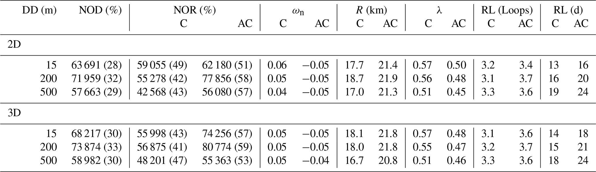
Table 2Statistics for drifters in 2D and 3D simulations containing ridges, showing the number of drifters (NODs) that contained ridges with corresponding percentages in parentheses of total drifters studied for the given deployment depth (DD; 15 m=225 732; 200 m=224 016; 500 m=195 624). As a drifter can experience several ridges, the number of ridges (NORs) is also given, separately for cyclonic and anticyclonic ridges together with their percentage in parentheses. The non-dimensional frequency (ωn), mean geometric radius (R) and ellipse linearity (λ) after averaging over all ridge points for the given deployment depth and simulation (2D or 3D) are also given. The ridge length (RL) is listed both as an average of the number of loops exhibited by the drifter containing the ridge and as an average of the number of days the drifters contain ridges.
The fraction of drifter data points with OW<0 is given based on an instantaneous count, but fractions are also shown after requiring that OW<0 should be reported by drifters for at least 1 or 2 consecutive days. With such temporal coherence criteria, the drifter-sampled OW<0 fraction drops. Finally, a split of any occurrence of OW<0 along drifter trajectories into cyclonic (positive relative vorticity) or anticyclonic (negative relative vorticity) reveal a systematic difference between the two polarities. These details will be discussed further in Sect. 4.1. Here we note that the fraction of OW<0 is about 6 times larger in the Eulerian fields than the fraction of ridge points found from the MWRA routine (compare solid green and black lines), which is about 6 %. The different spatial OW distributions, as well as the different fractions with negative OW from the Eulerian fields and the drifters, could imply that the drifters are not realistically entrained into the eddies. The drifters therefore might undersample the eddies. However, it is important to keep in mind that OW<0 is not a sufficient criterion to identify eddies, and the fraction of eddies from ROMS is an overestimate, hence likely closer to the estimates from the MWRA routine.
3.2 Vortex characteristics
We now focus on the coherent vortices found by the MWRA routine. Although the fraction of ridge points is relatively small, about 30 % of the drifters experiences ridges during their lifetime for all depths and simulations (see NOD in Table 2).
The number of ridges (NORs) after dividing into cyclonic and anticyclonic (Table 2) indicates more anticyclonic ridges than cyclonic ridges for all depths in both 2D and 3D simulations, with the exception for 2D drifters at 15 m, which have similar fractions of cyclonic and anticyclonic ridges. The vertical motion induced by strong atmospheric cooling, convection and mixing in winter, observed, e.g., in the 3D trajectories in Dugstad et al. (2019b), is not captured by the 2D drifters, and eddies are therefore sampled differently for 2D and 3D drifters deployed at 15 m. Deeper at 200 and 500 m the effect of surface cooling is weaker and the two simulations give similar results. We show results from 3D drifters in this section.
Relative frequency distributions (RFDs) of selected parameters are summarized in Fig. 5 for cyclonic and anticyclonic ridges separately. The RFDs for ωn indicate that vortices with different polarizations rotate with approximately the same angular frequency, which is slightly smaller for drifters deployed at 500 m (Fig. 5a). Compared to typical Rossby numbers of the LB region (see for instance Fer et al., 2018, and Søiland and Rossby, 2013, showing for the LBE), the values of ωn are fairly small. However, note that (see Table 1 for explanations of the variables), while the Rossby number in cylindrical coordinates is . The second term of this expression is not included in ωn and the quantities are therefore not directly comparable. We discuss this further below in this section. Using the mean geometric radius (R) as a proxy for the actual size of the associated eddies, we find that anticyclones are larger than cyclones. The ridge lengths are longer (both counted in days or in cycles) for the anticyclones (Fig. 5c and d), implying that anticyclones have a longer lifetime. The same result is obtained for the average values (Table 2). In addition, the ellipse linearity (λ) is smaller (indicating a larger amount of nonlinear vortices) for the anticyclones. Cyclones are relatively elongated, while anticyclones are circular and have larger radius at all depths.
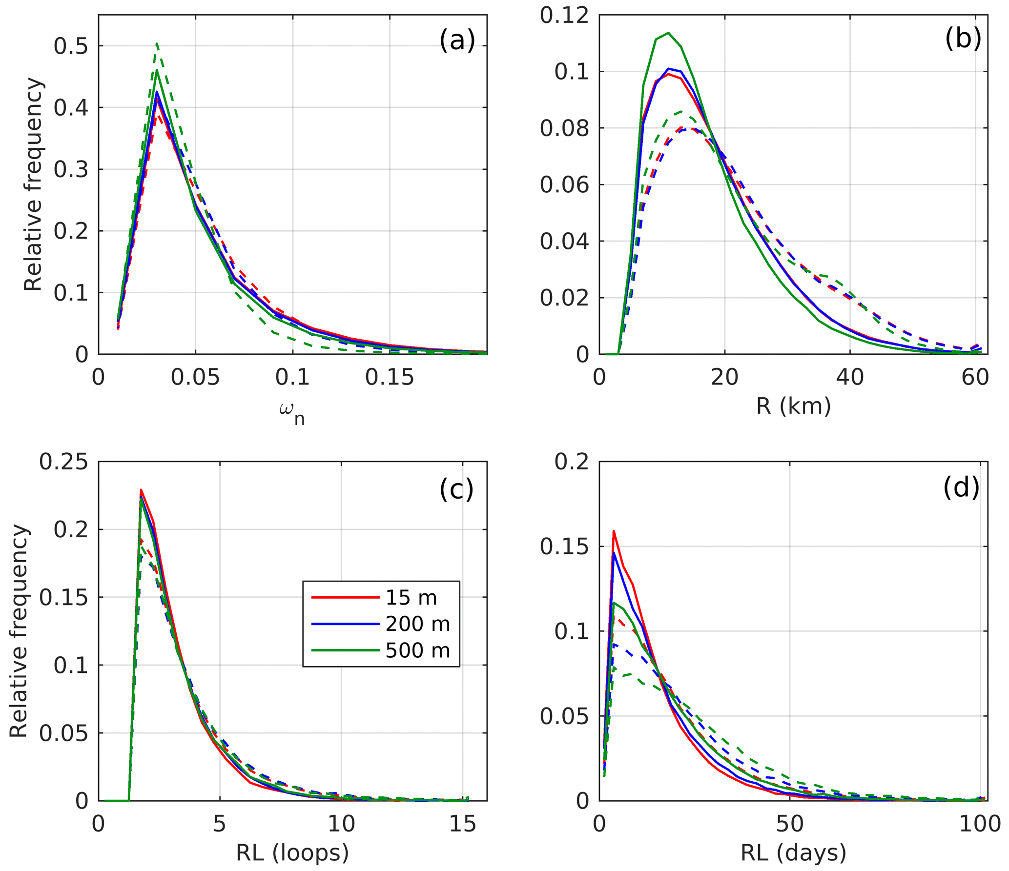
Figure 5Relative frequency distributions (RFDs) of (a) the non-dimensional frequency (ωn), (b) the mean geometric radius (R), i.e., the estimated instantaneous radius of the associated eddies, (c) the length of the ridges in cycles, RL (loops), and (d) length of the ridges in days, RL (days). RFDs are for all ridges found from the 3D drifters deployed at 15 m (red), 200 m (blue) and 500 m (green) and shown for both cyclonic ridges (solid) and anticyclonic ridges (dashed). The RFDs are created after binning each quantity and are normalized by the total number of cyclonic and anticyclonic ridge points, respectively.
The shape, size and lifetime of eddies depend on the regions where they are observed. Geographical distribution of ridges is estimated by obtaining density maps by counting the occurrences of ridge points in geographical bins of size (longitude bins are scaled with a factor similar to Dugstad et al., 2019b). Density maps (Fig. 6) for cyclonic and anticyclonic ridges are consistent with EKE maps from satellite altimetry (Volkov et al., 2013; Fer et al., 2020) and from observed drifter data (Koszalka et al., 2011), all showing the anticyclonic structure of the LBE and an anticyclonic secondary EKE maximum at the southeastern corner of the LB. Some anticyclonic ridges are found off the slope at all depths, particularly at 200 m. However, over the slope between the 1000 and 2000 m isobaths, cyclones dominate. As also noted by Ivanov and Korablev (1995) and Köhl (2007), there are cyclones around the anticyclonic LBE.
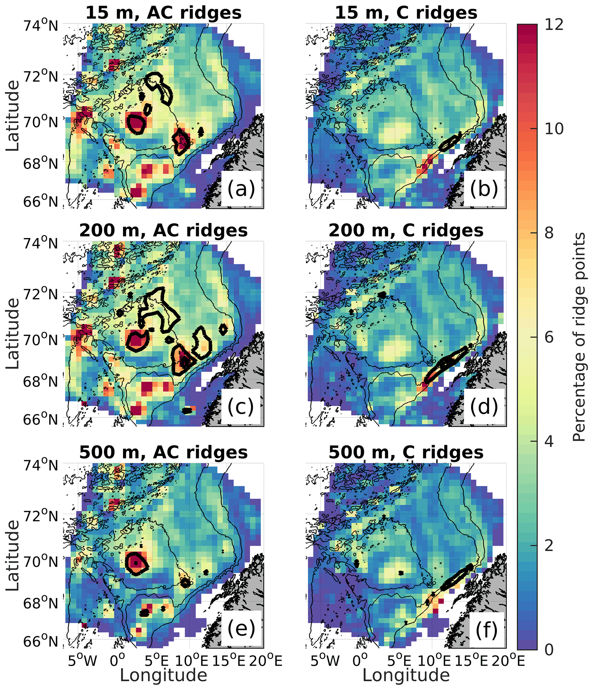
Figure 6Density distribution of (a, c, e) anticyclonic (ωn<0) and (b, d, f) cyclonic (ωn>0) ridges for 3D drifters deployed at 15 m (a, b), 200 m (c, d) and 500 m (e, f). The color bar shows the percentage of ridge points in each bin normalized to the total number of drifter data points in the same bins. Thin black contours show the 1000, 2000 and 3000 m isobaths, while thick black contours indicate key locations where the drifters are trapped into eddies, i.e., the first ridge point on each ridge. These contours are shown for more than 200, 300 and 400 first ridge points. A bin never contained more than 490 first ridge points. Bin sizes are .
The location of the first occurrence of a ridge in a trajectory is counted in the same geographical bins (thick black contours in Fig. 6). Anticyclonic ridges are often first found in the center of the basin where the LBE is located, close to the anticyclonic structure of the southeastern corner of the LB and sometimes off the slope, in agreement with earlier literature (Köhl, 2007; Koszalka et al., 2011; Isachsen, 2015). Over the slope (around the 1000 m isobath) cyclones appear to be generated more frequently. Note that the first ridge points may not always be representative of the eddy generation location, as on some occasions, the drifters could be deployed inside eddies. While this is likely the case in the permanent LBE, the large number of first ridge points near the slope may give a realistic distribution of generation sites.
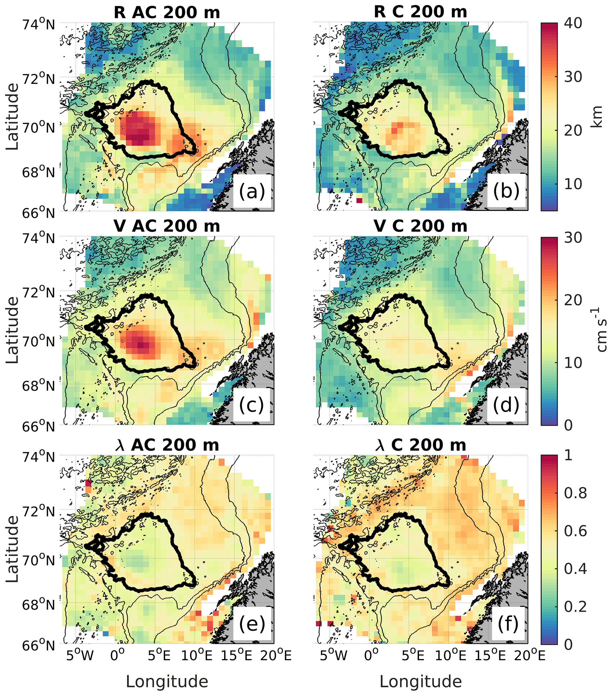
Figure 7Averaged (a, b) mean geometric radius (km), (c, d) orbital velocity (cm s−1) and (e, f) ellipse linearity for (a, c, e) anticyclonic and (b, d, f) cyclonic ridges from 3D drifters deployed at 200 m. Bin sizes are as in Fig. 6. Thin black contours show the 1000 and 2000 m isobaths and the thick black contour indicates the LB approximated by the 3000 m isobath. Note that V in (c) is negative but plotted with opposite sign for better comparison.
The spatial distributions of R, V and λ for anticyclonic and cyclonic ridges (Fig. 7) are presented for 3D drifters deployed at 200 m (other depths are similar). They are obtained by averaging the quantities for all ridge points in longitude–latitude bins. The largest eddies are anticyclonic and are found in the center of the LB associated with the LBE and with a mean geometric radius of 35–40 km, larger than the radius observed by Fer et al. (2018) (22 km) and Søiland and Rossby (2013) (18 km). However, they reported the radius of the maximum orbital velocities; hence drifters can loop around the LBE with a larger radius (i.e., on the flanks). The LBE is also characterized by large anticyclonic orbital velocity (about 30 cm s−1) and small ellipse linearity (about 0.3) (Fig. 7c and e). Note that due to large values of R, is enhanced relatively less in the LBE (about 0.07–0.08, not shown). We observe that the values of ωn in the LBE have magnitudes similar to the Rossby numbers computed about 35 km from the eddy core of the LBE from observations (Fig. 4a in Fer et al., 2018). As discussed earlier in this section, ωn is not directly comparable with the Rossby number, but similar magnitudes suggest that the drifters trace reasonable values at the given radius. The relatively small magnitudes of ωn in Fig. 5a therefore might be related to the fact that the drifters often loop on the eddy flanks. We also find anticyclonic ridges towards the southeastern corner of the LB and off the slope that have fairly similar properties to the LBE, i.e., increased orbital velocity and mean geometric radius and decreased ellipse linearity, indicating a stable character. Over the slope (1000 and 2000 m isobath) off the Lofoten Escarpment, the cyclonic ridges show smaller radii and a more elongated shape (higher λ), resulting in a more unstable character, possibly explaining why cyclones have shorter lifetime than anticyclones (Table 2 and Fig. 5d). The most stable cyclones appear to be in the center of the LB, probably surrounding the LBE, having an enhanced radius (Fig. 7b), slightly enhanced orbital velocity (Fig. 7d) and slightly decreased ellipse linearity (Fig. 7f).
3.3 Mean drift pattern of eddies and the ambient flow
The size, shape, nonlinearity, lifetime and generation sites of eddies influence the properties and fate of water masses trapped inside the eddies. How their water properties change with time can be related to processes within the eddies: how they drift, interactions with other eddies or the ambient flow, or how they are affected by the atmospheric forcing. Here and in Sect. 3.4, we study changes along drifter trajectories to investigate the drift of eddies as well as the evolution of their water masses with time. We compare this with the ambient flow (the AF drifters). We obtain the mean drift of eddies and the ambient flow (Fig. 8) by averaging all velocities into longitude and latitude bins. We show results at 200 m to be consistent with earlier results. Eastward and northward velocities are computed along ridges from the rate of change in position using the lonres and latres variables (Table 1), which give the position of the mass center of the eddy, and for the AF drifters, their longitude and latitude data are used. The velocity fields from ridges give the mean eddy drift (Fig. 8b and c). We also obtain the residual eddy drift by subtracting the Eulerian mean flow obtained from the ROMS model given in Fig. 8a, for both cyclonic (Fig. 8e) and anticyclonic ridges (Fig. 8f), as well as for the AF drifters (Fig. 8d). Note that the velocity fields are derived from the 2D drifters to ensure that they are at fixed levels (200 m).
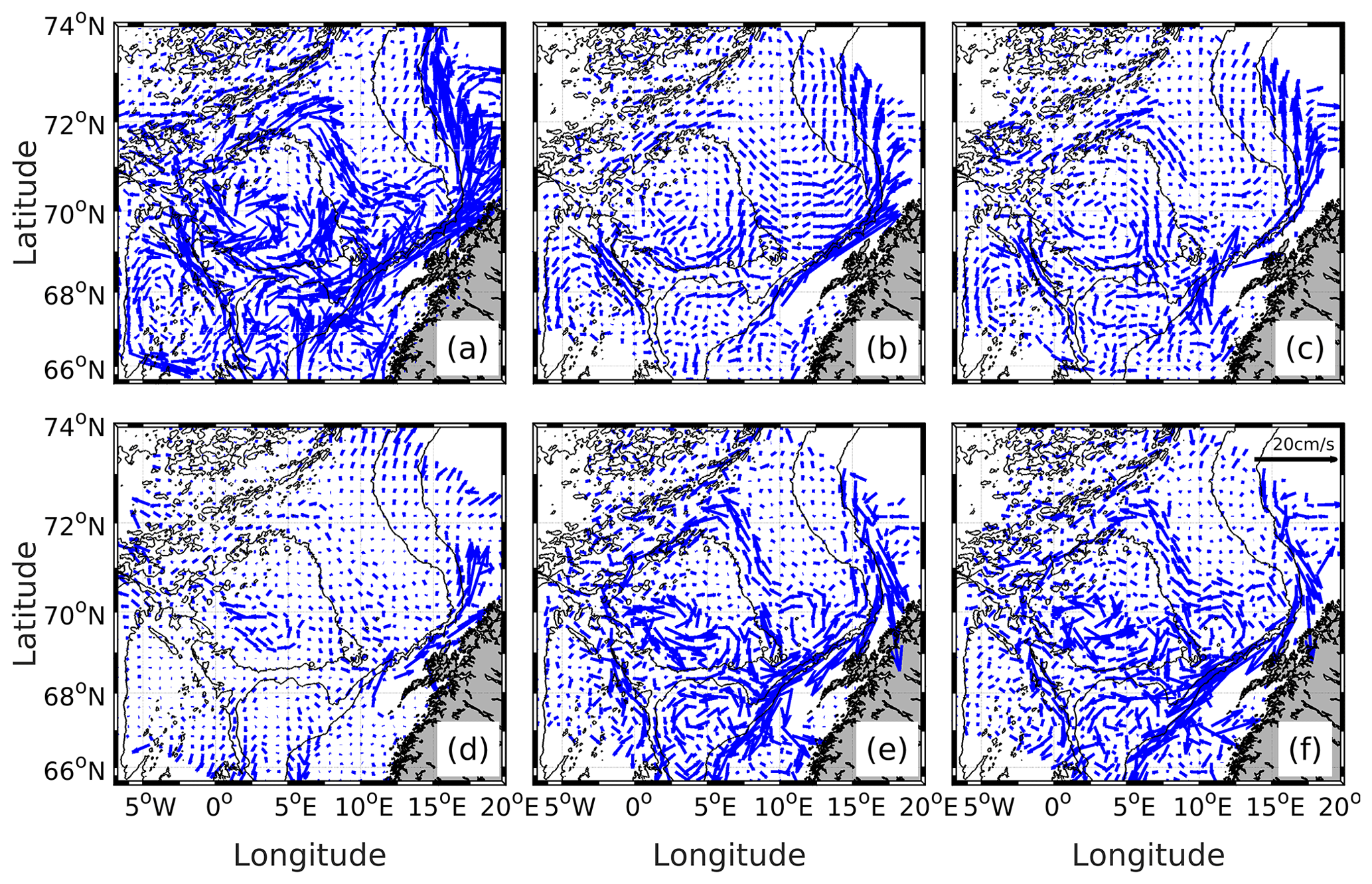
Figure 8Averaged velocity fields at 200 m from ROMS or 2D drifters. (a) Eulerian mean flow from the ROMS model at 200 m averaged between 1996 and 2000; (b) drift of cyclonic ridges; (c) drift of anticyclonic ridges. Residual flow from (d) AF drifters, (e) cyclonic ridges and (f) anticyclonic ridges. Residuals are obtained by removing the Eulerian mean flow (a). Scale of the arrows is given in upper right in (f) and is the same for all panels
The AF drifters on average follow the Eulerian mean flow from the ROMS model (i.e., residual drift of the AF flow is small) (Fig. 8d). The cyclones and anticyclones exhibit a fairly similar drift, with smaller magnitude than the Eulerian mean flow (Fig. 8b and c). This results in large magnitudes of the residual eddy drift for both cyclones (Fig. 8e) and anticyclones (Fig. 8f). The slower drift of the cyclones and anticyclones is particularly pronounced on the slope with residual currents of 15–20 cm s−1 pointing southwards against the direction of the mean flow. Water masses in eddies therefore tend to experience increased residence time in the LB region and a longer transit time towards the Arctic, possibly leading to larger changes in water mass properties compared to the ambient flow (further discussed in Sect. 3.4). We observe that the mean flow is weaker towards deeper levels (500 m) compared to 15 and 200 m (not shown). However, the eddy drift speeds have a fairly similar pattern at all levels. This indicates that the eddies at 500 m drift with a speed similar to the mean flow, but at 15 m, the eddy drift is relatively slower.
3.4 Evolution of water masses in eddies and in the ambient flow
The AW modification is particularly strong in regions with large eddy activity, such as the LBE and the secondary EKE maximum in the southeast of the LB (Rossby et al., 2009a; Bosse et al., 2018). In this section, we attempt to quantify the evolution of temperature, density and vertical displacements along ridges and AF drifters, to estimate the property rate of change in a water parcel inside an eddy compared to the ambient flow.
We first estimate the characteristic temperature anomalies for the cyclonic and anticyclonic ridges and compare these to AF drifters. To remove the spatial and seasonal variability embedded in the drifter temperatures, we compute a background temperature climatology from the ROMS model by taking seasonal averages of temperature for winter (January–March), spring (April–June), summer (July–September) and fall (October–December) between 1996–2000, the same period as the Lagrangian simulations. These are interpolated onto the drifter trajectories and subtracted from the temperatures to give temperature anomalies. The RFDs of anomalies from the 3D drifters (Fig. 9) indicate that anticyclones are warm and cyclones are cold compared to the background flow, consistent with results obtained from Argo floats (Raj et al., 2016). The RFDs are also centered around larger positive and negative values with depth for anticyclones and cyclones, respectively (mean of 0.19 and 0.37 ∘C at 15 and 500 m, respectively, for anticyclones and mean of −0.25 and −0.33 ∘C at 15 and 500 m, respectively, for cyclones), consistent with results obtained from hydrography (Sandalyuk et al., 2020). For the ambient flow (AF drifters), the temperature anomalies are centered around zero.
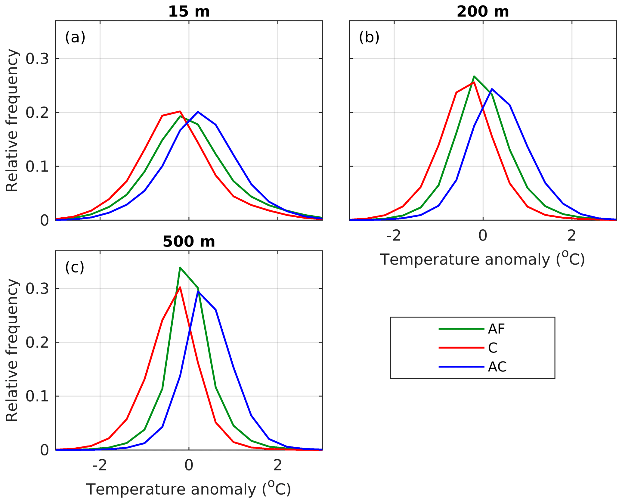
Figure 9RFDs of temperature anomalies for 3D drifters deployed at (a) 15 m, (b) 200 m and (c) 500 m. The anomalies are relative to a seasonal background climatology from the ROMS fields (see text). RFDs are shown for AF drifters (AF, green), cyclonic ridges (C, red) and anticyclonic ridges (AC, blue).
Warm and cold temperature anomalies for anticyclones and cyclones, respectively, can impact the cooling and warming experienced by water masses inside them. Since cooling and warming are related to an increase or decrease in density, this may also affect the vertical motion of the water masses. We therefore compute daily temperature changes and vertical displacements along drifter trajectories and assign these values to the drifter's mean position that day. With a lifetime of 1 year this is 364 data points for each drifter or less if a drifter runs aground or exits the domain earlier. The daily temperature changes and the vertical displacements for 3D drifters are then binned as before.
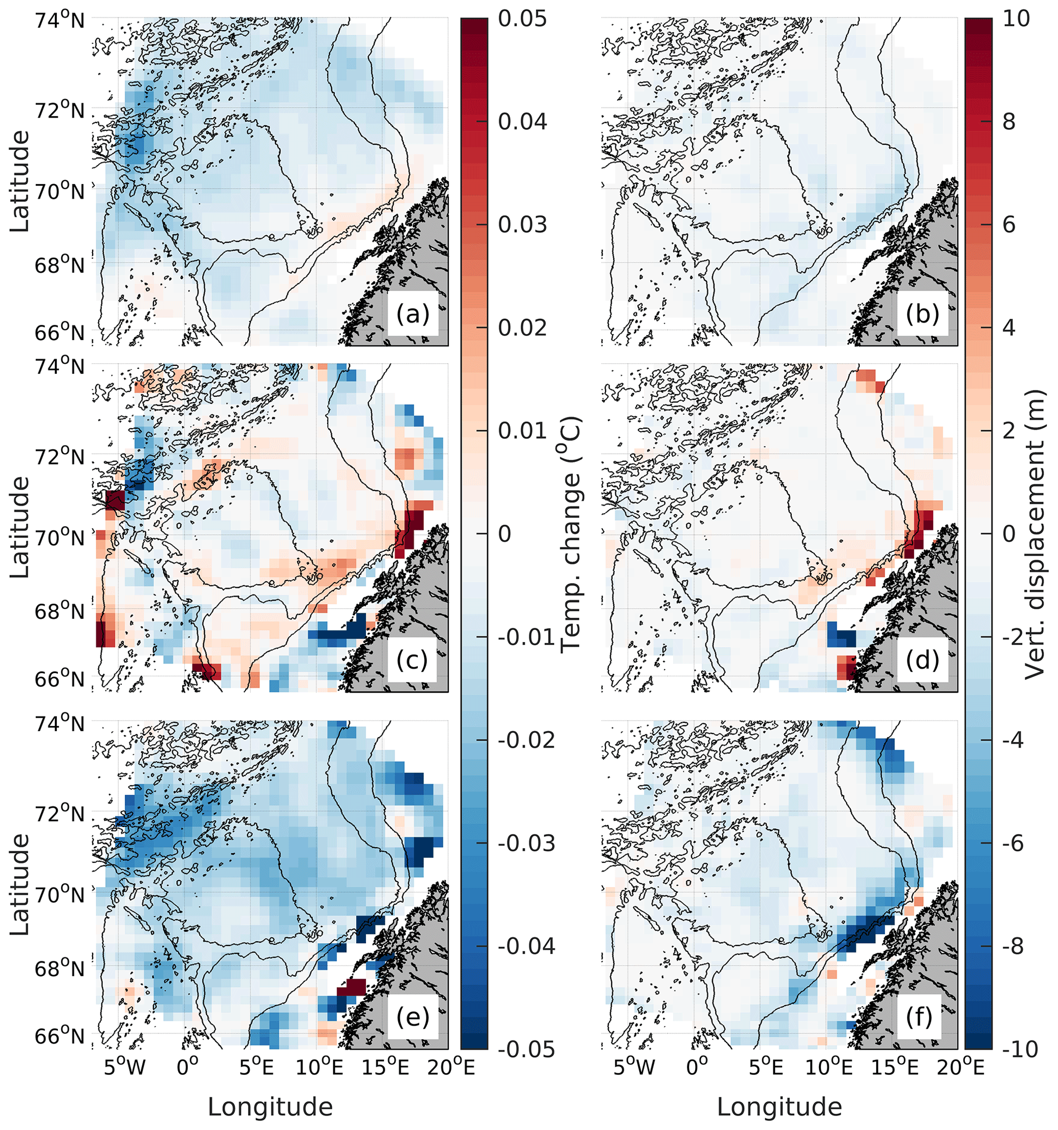
Figure 10Averaged (a, c, e) daily temperature changes and (b, d, f) daily vertical displacements (colors) computed for (a, b) AF drifters, (c, d) cyclonic ridges and (e, f) anticyclonic ridges for 3D drifters deployed at 15 m. The maps are smoothed using a nine-point mean filter to remove some noise.
For 3D drifters deployed at 15 m (Fig. 10) there is an overall net cooling and sinking in the domain, with the largest values for the anticyclonic ridges (e, f). Along the cyclonic ridges (c, d) the drifters experience some warming (0.01–0.02 ) and upward motion (2–4 m d−1) by the slope but cooling in the basin (0–0.01 ), likely reflecting the atmospheric cooling close to the surface. For the 3D drifters deployed at 500 m (Fig. 11) there is typically enhanced cooling and downwelling in the anticyclones and enhanced warming and upwelling in the cyclones. However, while there is a fairly consistent pattern of cooling (anticyclones) and warming (cyclones) in the domain, the vertical displacements vary geographically. For the AF drifters the temperature and depth changes are generally small, except at the surface where they lose temperature and sink in response to atmospheric cooling.

Figure 11As in Fig. 10 but for 3D drifters deployed at 500 m.
There is no obvious relation between the temperature changes and the vertical motion in the different flow categories (Figs. 10 and 11); i.e., we cannot say that a change in temperature leads to a change in the vertical displacement. Note also that the results are based on daily differences and should be interpreted with caution. For instance, a water parcel entering the LBE from a colder environment could initially experience warming, but over longer timescales water masses in the LBE are generally cooled. It is therefore of interest to study how water masses in eddies and in the ambient flow change over a longer period of time. Since the 2D drifters remain at their deployment depth, a comparison with the 3D drifters provides information about the effect of the temperature change on vertical motion or vice versa. We focus on the LB and compute time series of the temperature and density change and vertical displacements along all drifter trajectories inside the basin. Using all drifters that interacted with the LB (either deployed there or entered at a later time), we calculate the temperature differences Ti−T1 (and density differences and vertical displacements similarly) for all trajectories while they are in the basin. Ti and T1 denote the temperature at index i and index 1 along a drifter trajectory after it entered or was deployed in the LB. If a drifter crosses the basin boundary multiple times, each period in the basin is considered separately. This gives a record of how the properties change with time for each drifter segment inside the basin. Averaging over all drifter segments studied for every time step, we obtain a time series of the mean property change in the basin. This procedure is done for cyclonic and anticyclonic ridges and for AF drifters. To look at whether the LB is important, we also perform a similar analysis for comparison, using all drifters in the entire domain and computing differences along all trajectories from deployment to termination.
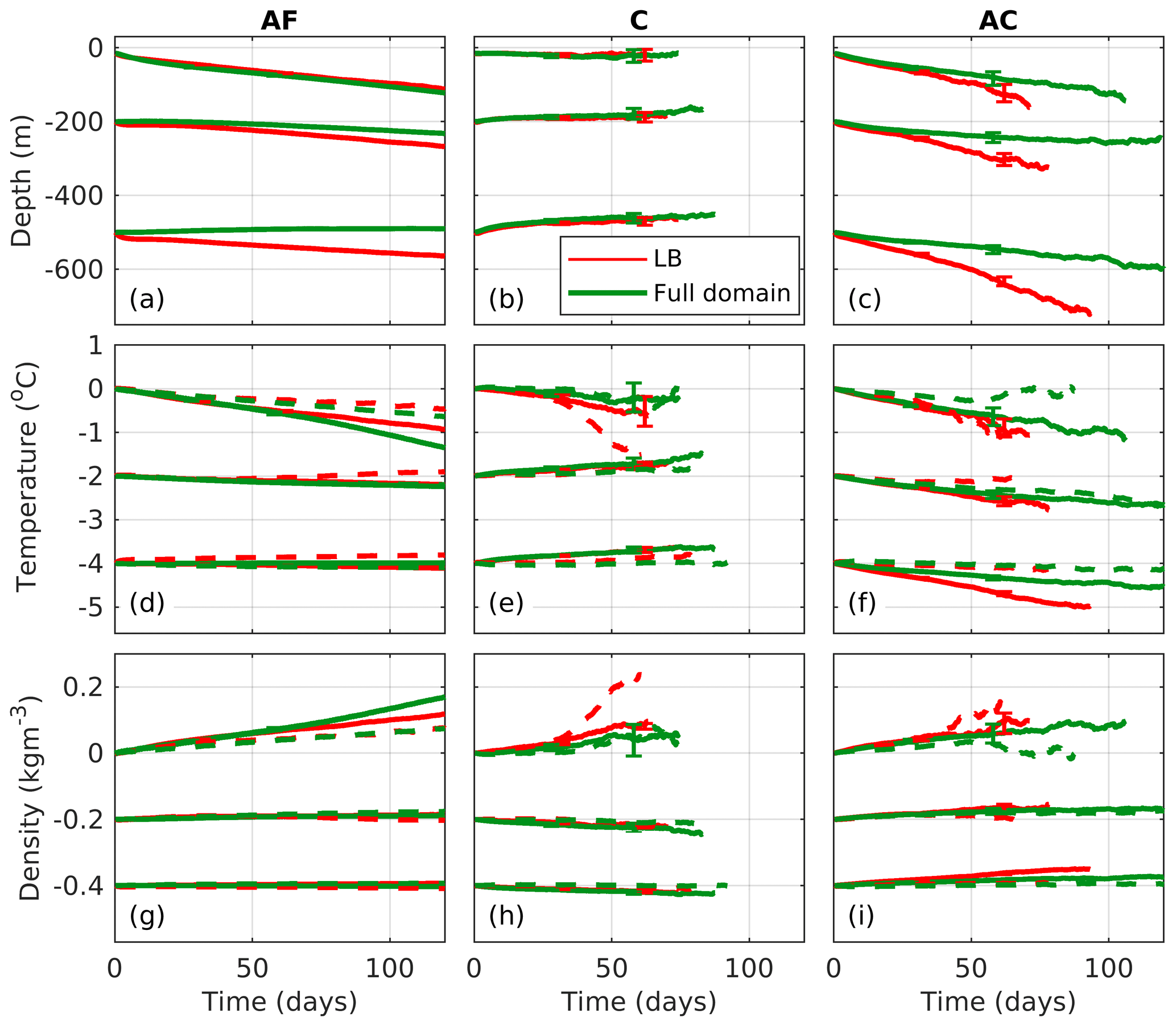
Figure 12Time series of (a–c) mean vertical displacement for 3D drifters, (d–f) mean temperature change and (g–i) mean density change for 2D (dashed) and 3D (solid lines) drifters. Analyses for the LB (red) and the full domain (green) are shown for the (a, d, g) AF drifters, (b, e, h) cyclonic ridges (C) and (c, f, i) anticyclonic ridges (AC), and for different deployment depths (15, 200 and 500 m). To distinguish the drifters that were deployed at 15, 200 and 500 m, an offset of −15, −200 and −500 m is used for the vertical displacements, 0, −2 and −4 ∘C for the temperature changes, and 0, 0.2 and 0.4 kg m−3 for the density. The mean is based on fewer data points with increasing time, and time series are therefore stopped when the mean is based on fewer than 100 data points. Error bars given as twice the standard error of the mean are given at day 30 and 60 for both the LB (red) and the full domain (green). These are distinguished by using offsets of +2 d for red and −2 d for green. Error bars are only included for the 3D particles.
The vertical displacements indicate a net sinking in the domain for the ambient flow, and this is even more enhanced in anticyclones (Fig. 12). Error bars showing twice the standard error of the mean (to indicate 95 % significance) plotted at day 30 and 60 after the drifters entered the LB are also included. Note that these are plotted for cyclonic and anticyclonic ridges and for the AF drifters, but due to their small magnitudes they are hardly visible for the AF drifters. Small error bars indicate that the vertical displacements are significant. Water masses in cyclones on average stay at fixed depths with time, but there is some upward motion at 500 m. The mean sinking is more pronounced in the LB compared to the full domain. Due to the initially warm signature of anticyclones, we observe a net cooling within these (and the opposite for cyclones), which again is mainly enhanced in the LB (Fig. 12e and f). Cooling is also experienced by the AF drifters, but this is most pronounced close to surface, possibly due to a stronger atmospheric cooling there. Despite some differences, 2D and 3D results agree fairly well: 2D cyclonic ridges at 15 m cool strongly in the LB compared to the 3D cyclonic ridges. Since the 2D drifters are close to the surface during their entire lifetime, they are exposed to atmospheric cooling for extended periods compared to 3D drifters that are vertically spread and can enter a cyclone at deeper levels. Also, for the anticyclones the 3D drifters deployed at 200 and 500 m experience more cooling and density increase than the 2D drifters, especially in the LB.
Cooling of the water parcels is typically accompanied by an increase in density (Fig. 12g–i). In these cases, a net sinking also often occurs, for example for water masses in anticyclones in the LB at 200 and 500 m. However, there are also examples of sinking, not associated with cooling or increase in density, for instance for AF 3D drifters in the LB deployed at 500 m (Fig. 12a, d and g). In this case the vertical motion could be related to movement along isopycnals that on average deepen due to weak stratification in the LB (e.g., Bosse et al., 2018). The vertical motion of the 3D drifters is discussed further in Sect. 4.2.
3.5 Temperature and vorticity fluxes into the LB
The temperature and density changes are stronger in the LB compared to the full domain (Fig. 12), consistent with earlier literature indicating that the LB is an important region for heat loss to the atmosphere and modification of AW (Rossby et al., 2009a; Richards and Straneo, 2015; Bosse et al., 2018; Dugstad et al., 2019a). The net heat flux into the basin has previously been found to be positive from Eulerian calculations using both observations and model simulations (Segtnan et al., 2011; Dugstad et al., 2019a). Here we have observed that the cooling rate in the anticyclones (experienced by drifters) are enhanced (Figs. 10–12), and we intuitively expect that water parcels in anticyclones will contribute considerably to heat fluxes into the LB. However, the small fraction of ridge points suggests that, summed over all water parcels, the total contribution from the ambient flow could be substantial. As noted earlier, idealized simulations made by Spall (2010) have already indicated that filaments can be important in providing positive vorticity fluxes into the LB. We therefore proceed to make a drifter-based estimate of the relative contribution of vortices and ambient flow to net heat and vorticity fluxes into the LB. In our analysis, ridges will be a proxy for coherent vortices and AF drifters a proxy for both the mean flow and filaments. Note also that we will report temperature fluxes rather than heat fluxes since we focus on relative rather than absolute contributions.
To calculate the net temperature and vorticity fluxes into the LB, we tag all drifters that passed through the basin (so both entering and exiting). The net fluxes are then computed as the difference between fluxes in and fluxes out for each drifter. Note that a drifter can enter and exit the LB several times, and we thereby compute fluxes for all drifter segments in the basin. We interpret each drifter as carrying a given mass, and by doing the calculation only on drifters that entered and then exited the basin the calculation approximately conserves mass. For each entry/exit we obtain the values of temperature T and velocity and estimate the temperature flux into or out of the basin as , where n is the local normal vector to the basin contour (pointing inwards so that entries are positive). For each drifter segment the net temperature flux is then computed as TFin−TFout.
The drifters can enter and exit as ambient flow, anticyclones or cyclones. However, it is possible that a drifter changes its category in the basin, meaning that it may for instance enter while being trapped within an anticyclone but exit as part of the ambient flow. We are interested in whether such transitions may play a role in the dynamics and therefore separate the calculations of TFin−TFout into six categories: ambient flow in, anything out (AFi); anticyclones in, anything out (ACi); cyclones in, anything out (Ci); anything in, ambient flow out (AFo); anything in, anticyclones out (ACo); anything in, cyclones out (Co). The categories are defined such that the total number of drifter segments in the AFi, ACi and Ci categories equals the total number of drifter segments in the AFo, ACo and Co categories. Furthermore, since the drifters are deployed in 1996, 1997 and 1998 with roughly the same number of drifters deployed each year, we compute net temperature and vorticity fluxes for drifters deployed in each of these years. From these 3 years we thereby compute a mean temperature and vorticity flux together with standard errors. The results are shown in Fig. 13 with error bars given as twice the standard error to indicate 95 % confidence intervals. Note that the total fluxes summed over the AFi, ACi and Ci categories equal the fluxes summed over the AFo, ACo and Co categories for each year. However, for the 3-year mean there will be small differences since the number of drifters interacting with the LB is only approximately the same each year.
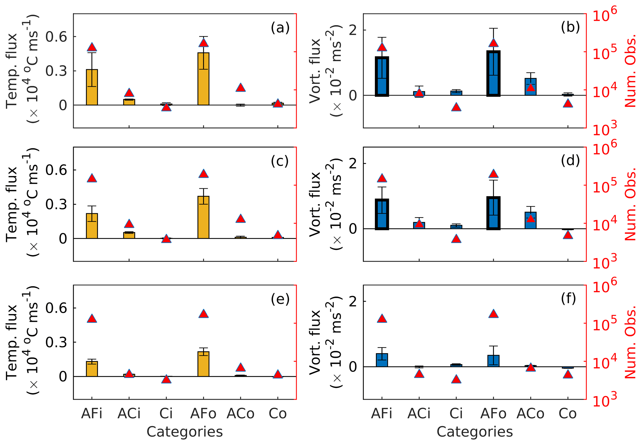
Figure 13Estimates of the (a, c, e) net temperature flux and (b, d, f) net vorticity flux into the LB for 3D drifters deployed at (a, b) 15 m, (c, d) 200 m and (e, f) 500 m depth. The results are shown for selected entry/exit pair categories described in Sect. 3.5. Thick black edges on AFi and AFo bars in (b) and (d) indicate that these are shown as one-third of their original size. Red triangles show the number of drifter pairs used for the calculation and are given on the right axes with a log scale. The abbreviations are as follows: AFi – ambient flow in-anything out; ACi – anticyclone in-anything out; Ci – cyclone in-anything out; AFo – anything in-ambient flow out; ACo – anything in-anticyclone out; Co – anything in-cyclone out.
Summed over all categories, the net temperature flux into the basin is positive (Fig. 13a, c and e). The magnitude of the temperature fluxes for ACi is larger than for Ci (13 a, c and e), consistent with positive and negative temperature anomalies for anticyclones and cyclones, respectively (Fig. 9). But the calculation clearly indicates that the AFi and AFo categories dominate the total flux. We note that if a drifter enters the LB as part of the ambient flow, only about 2 % of these drifters will experience a transition to exit as part of a cyclone or anticyclone (not shown). Most drifters in the AFi and AFo categories therefore also exit or enter as part of the ambient flow, respectively. The integrated effect of the ambient flow is therefore more important than eddies for the net temperature flux. Considering the ridge categories, we note that about 22 % of the drifters that enter the basin in an anticyclone experience a transition to exit as another category, and the corresponding fraction is 28 % for cyclones. Looking at exits, the numbers are similar: 22 % of the drifters exiting in an anticyclone entered as something else, while 27 % of the drifters exiting in a cyclone entered as something else. Closer inspection reveals that the drifters can experience a transition from an anticyclone or cyclone to the ambient flow (or vice versa), but the transition from anticyclone to cyclone or vice versa is almost non-existent (less than 1 % of the cases).
The net vorticity flux into the basin is positive and is also dominated by the AFi and AFo categories (Fig. 13b, d and f). This dominance is overwhelming for drifters deployed at 15 and 200 m but less so for those deployed at 500 m depth. We discuss this further in Sect. 4.3. Perhaps counterintuitively, we observe positive vorticity fluxes for the ACi category for drifters deployed at 15 and 200 m but believe this is due to the fact that about 73 % of the drifters entering as part of anticyclones also exit as anticyclones. At 500 m, negative vorticity fluxes for ACi and Co indicate that drifters entering in an anticyclone or drifters that exit in a cyclone are on average associated with a negative vorticity change in the basin.
The number of observations is also given in Fig. 13. The dominance of AFi and AFo is clearly related to the larger number of available drifters from this category that go into the calculations. The net temperature fluxes into the basin per drifter segment are 0.01–0.02 for AFi, 0.04–0.06 for ACi and 0.0–0.3 for Ci for all depths with the largest values close to the surface. This indicates that a single drifter experiences the largest temperature drop when it enters the LB in an anticyclone. The “out” categories have similar magnitudes except for the ACo category where the magnitudes are 4–10 times smaller than for the ACi category. A similar pattern is seen for the vorticity fluxes: one single drifter experiences a larger change in vorticity when it enters or exits with a cyclone or anticyclone compared to a drifter that enters with the ambient flow. The results are thus sensitive to the choice of studying the net fluxes over all drifter segments or per drifter segment. We discuss this further in Sect. 4.1.
Recall that the AF category includes anything which is not classified as coherent vortices, such as the mean flow, filaments and other submesoscale features. Spall (2010) found that filaments could often carry large cyclonic vorticity (sometimes with ζ=2f) and suggested that these could give large fluxes into the basin. So at this point we hypothesize that the large fluxes into the basin from the ambient flow in our study are related to filaments. If focusing on the ambient flow and more specifically on the AFi category, we first note that the mean net vorticity flux into the basin for a drifter is positive and that the magnitude is only 2–3 times smaller than for drifters in the ACi category (see previous paragraph). Considering the RFD of the associated net vorticity fluxes into the basin for the AFi category (not shown), a skewness of 1.4, 1.7 and 2.4 for drifters deployed at 15, 200 and 500 m, respectively, is observed. This implies a skewness towards a positive net vorticity flux and that the RFDs have longer tails towards positive values compared to negative values. This together with a positive mean could point to the fact that the vorticity fluxes computed from the ambient flow are related to several features such as filaments and other submesoscale flow in addition to the mean flow. We will discuss this further in Sect. 4.3.
4.1 Eddy sampling by the drifter trajectories
The relatively small fraction of ridge points (6 %) in the drifter trajectories suggests that drifters spend most of their time outside of coherent eddies. A comparison of the Lagrangian and Eulerian OW maps (Fig. 4a and b) also indicates that the fraction of drifter data points sampling OW<0 are generally smaller than the fraction of grid cells in the model that have OW<0. The two estimates are similar early in the deployment (Fig. 4c), suggesting that uniformly deployed drifters (that could be deployed in eddies or the ambient flow) reflect the Eulerian OW field of the model in the beginning. With time, however, the fraction of drifters sampling OW<0 rapidly decreases, and after 15–20 d it stabilizes around 34 %–35 %, some 5 %–6 % lower than the Eulerian-based estimate. This initial adjustment may be tied to the secondary circulation within coherent vortices. In particular, Bashmachnikov et al. (2018) found that such circulation within the LBE (an anticyclone) consisted of a divergent horizontal flow in and above the vortex core. Assuming such secondary circulation occurs in other anticyclones and that the flow pattern is opposite for cyclones, this effect could result in an initial drop of the OW<0 fraction with negative vorticity sampled by drifters and an initial increase for positive vorticity. At later times, drifters may experience potential vorticity (PV) barriers that prevent them from entering into the core of eddies. Such barriers, associated with strong PV gradients, have been shown to exist, for example, around the LBE from cruise data and RAFOS floats (Bosse et al., 2019). The anticyclonic eddies in this study have a longer lifetime and a more circular shape, likely reflecting more nonlinear motion. The PV barriers are therefore likely stronger for the anticyclones than the cyclones, possibly explaining why the fraction of drifters experiencing OW<0 with negative vorticity is smaller than that with positive vorticity (Fig. 4c).
So at late stages after deployment, more drifters experience OW<0 with cyclonic vorticity compared to with anticyclonic vorticity (red vs. blue dashed lines in Fig. 4c). This may seem contradictory to what we find with the MWRA routine, as this detects more anticyclonic ridges (Table 2), a result which is consistent with findings reported by Raj et al. (2016) and Volkov et al. (2015). But here it is worth noting that the criterion of OW<0 is not thought to be sufficient for identifying coherent vortices (Penven et al., 2005; Raj et al., 2016; Trodahl and Isachsen, 2018). So the relative fraction of drifter-sampled positive and negative vorticity, even where OW<0, likely also reflects other flow features. In particular, the surrounding flow around anticyclones is typically dominated by cyclonic filamentary structures (not shown, but see, e.g., Spall, 2010). We therefore speculate that drifters to a large extent sample filaments with cyclonic vorticity in the vicinity of the (more numerous) anticyclones.
The MWRA detects long-lived coherent eddies by design, requiring sustained looping by drifters. The most sensitive parameter choice in this routine is the choice of minimum ridge length (RL). For the above analysis we used an RL of 3.1 cycles (Sect. 2.3), but as a sensitivity experiment we ran the MWRA routine with the RL set to 1.6 cycles, similar to Lilly et al. (2011). For this test we only used 10 000 randomly chosen drifters to reduce computation time. The shorter minimum ridge length resulted in 65 %–70 % more ridge point detections (Fig. 4c, other depths and simulations show similar results). But we note that RL = 1.6 is similar to the number of oscillations within the wavelet and therefore on the limit of a meaningful eddy signal. As the wavelet transform is a joint function of the wavelet and the trajectory signal, noise or smaller jumps in the trajectories could lead to copies of the wavelet itself in the wavelet transform (Lilly and Olhede, 2009; Lilly et al., 2011). Hence, the sensitivity experiment discussed here should be interpreted with caution. Conversely, with some temporal coherence as a definition for eddies in mind, it is interesting to note that the fraction of drifter data points that sample OW<0 for more than 1 or 2 d decreases drastically compared to a detection based on instantaneous OW values (green dashed lines in Fig. 4c). In fact, the OW-based and ridge-based drifter estimates then start to converge. Putting additional constraints on eddy detection based on the Eulerian ROMS fields would likely lead to an additional decrease in the computed fractions.
The indications shown in Fig. 13 that the ambient flow (AFi and AFo categories) dominates both temperature and vorticity fluxes into the LB need to be interpreted in the light of the above discussion. If one takes the stand that the MWRA routine grossly underestimates the prevalence of coherent vortices and that OW<0, calculated from Eulerian fields, is instead a true indicator, then the relative flux estimates would be off by a factor of about 6 (as the green solid line in Fig. 4 is about 6 times higher than the black solid line). But note that as the flux values of the ACi, Ci, ACo and Co categories are based on about 10 000 drifter segments each, while the AFi and AFo categories are based on about 130 000 drifter segments each, a 6-fold increase in ACi, Ci, ACo and Co (giving 60 000 drifter segments) would lead to a decrease to about of the results shown for the AFi and AFo categories (which would then include 80 000 drifter segments). In this limiting case the net temperature flux into the basin would indeed be dominated by the ridge categories. But the AFi and AFo categories would still play an important role and even more so for the vorticity flux. And since using OW<0 alone as a criterion for coherent eddies is clearly unrealistic and we expect the actual fraction of coherent eddies to be more similar to the estimates from the MWRA routine, we conclude that the ambient flow is important for a balanced heat and vorticity budget.
4.2 Change in water properties in eddies and the ambient flow
The eastern Nordic Seas that we study here are primarily temperature-stratified. We hence expect that water parcels that are cooled will eventually sink from gravitational adjustment. An indication that this process is taking place near the surface, where parcels are directly exposed to air–sea heat loss, is seen in Fig. 12 for the 3D AF (ambient water) and AC (anticyclones) drifter classes seeded at 15 m. Generally, 2D drifters seeded at the same depth experience smaller temperature drops (and density increases) than do 3D drifters. A plausible interpretation is that the fixed-level drifters are not allowed to gravitationally adjust along with the coldest waters that they encounter. Vertical motion of 3D drifters that coincide with changes in temperature and density which are larger than for 2D drifters is also seen at depth and in particular for drifters in anticyclones in the LB. However, examples of vertical motion not accompanied by changes in temperature or density also occur, for instance for the AF drifters in the LB deployed at 200 and 500 m. The vertical motion experienced by these drifters in particular, but partly also the other drifter classes, may reflect adiabatic movement along sloping isopycnals. The pronounced sinking experienced by 3D AF drifters at depth in the LB compared to the full domain can partly be related to the deepening of isopycnals observed there (Rossby et al., 2009a; Bosse et al., 2018).
The most pronounced signal seen in Figs. 10–12 is perhaps the asymmetry in what drifters experience in cyclones and anticyclones. Drifters trapped in anticyclones mostly experience downward motion, while those in cyclones mostly experience upward motion (drifters in cyclones do not sink near the surface like AF and AC drifters do). The vertical movement here too may be reflecting gravitational adjustment resulting from the cyclones gradually warming up (as they are anomalously cold) and the anticyclones gradually cooling. But some of the asymmetry may also be related to the secondary circulation within vortices mentioned in Sect. 4.1. Bashmachnikov et al. (2018) found from model studies using MITgcm that vertical motion in the LBE has a complex structure with a lateral divergence of water masses at upper levels, leading to upward motion in and above the eddy core. This is compensated for by downward motion along the flanks of the vortex. If such a secondary circulation pattern is common for anticyclones in the LB – and the opposite for cyclones – then our drifter statistics should be affected systematically. We deploy drifters uniformly, sometimes in the eddy cores but most often outside eddies (since the eddies cover a smaller portion of the domain than the ambient flow). Although some drifters occasionally enter eddy cores, our results indicate that they spend a larger fraction of their time on ridges outside the cores. In particular, we found that ridges in the LBE typically trace out radii that are significantly larger than the core radius reported by Fer et al. (2018) and Søiland and Rossby (2013), implying that these drifters were often looping on the eddy flanks. We therefore speculate that some of the observed downwelling of drifters in anticyclones and upwelling in cyclones is related to the secondary circulation within the vortices. It is worth noting that vertical advection by such secondary circulation through the stably stratified water masses in and around a vortex will lead to the kinds of temperature and density changes recorded by our synthetic 3D drifters. In steady state the vertical advection must, in turn, be balanced by turbulent buoyancy fluxes. This requirement is at least indirectly supported by observational reports of enhanced turbulent dissipation levels within the LBE (Fer et al., 2018).
So the observed vertical motion of water masses in and around the LB can therefore be related to several processes. On the one hand, cooling and densification can cause subduction, but only if the water masses get heavier than their surroundings. The vertical motion can also be related to motion along sloping isopycnals. For eddies, a secondary vertical motion within the eddy may also occur. In the first and third case the water masses change their properties and exhibit water mass transformation, while the second case is adiabatic. We propose that actual water mass transformation takes place mainly near the surface but also in vortices at depth since here too the 2D and 3D temperature and density changes are different.
4.3 Vertical structure in the AW–LB exchange
The fact that the ambient flow dominates the net vorticity fluxes (and temperature fluxes) into the LB is consistent with the idealized model simulations of Spall (2010) and points to the importance of filaments. If the ambient flow was dominated by the mean flow, this could not explain the large magnitudes in Fig. 13b and d. We also find it reasonable to believe that the huge difference in the net vorticity fluxes between drifters deployed at 15 and 200 m compared to 500 m is a result of filaments. This points to a more dynamically active surface than at deeper levels, likely caused by more variability due to wind and surface buoyancy fluxes. That the net vorticity fluxes are positive and that the RFDs are positively skewed (Sect. 3.5) is also consistent with the fact that the eddies found by the MWRA routine were dominated by anticyclonic rotation. Following the discussion in Sect. 4.1, this could possibly indicate that many drifters in the ambient flow traced filaments with positive values of relative vorticity around the anticyclonic eddies. The anticyclones and cyclones have a shorter lifetime at the surface than at deeper levels and are more elongated (Table 2 and Fig. 5d), implying a more unstable character. We speculate that variable wind fields at the surface disturb the generation of eddies and that enhanced diapycnal processes drain energy and limit the lifetime of vortices but favor the occurrence of filaments.
As mentioned above, at 500 m, the vorticity fluxes tied to the ambient flow are smaller than at surface and 200 m depth (Fig. 13f, about one-third of the results at 15 and 200 m). The same is also partly true for the temperature fluxes. Since the magnitudes associated with the ridge categories are more or less similar for all depths, this implies a relatively larger contribution of fluxes related to vortices at deeper levels. Focusing on the temperature fluxes, earlier studies have suggested that a divergence of eddy heat fluxes from the continental slope towards the basin interior dominate at subsurface levels (Dugstad et al., 2019a). The eddies at depth have longer lifetimes (Table 2 and Fig. 5) and about the same drift speed as eddies at shallower levels (not shown), meaning they are likely to propagate over longer distances and reach the basin. Given that the anticyclones are warm and often detected close to the basin (not at the slope, Fig. 6), these can therefore drift to the basin feeding the LB with warm water. Considering only the anticyclonic entries to the LB from drifters deployed at 500 m, about 41 % from 3D drifters occur along the southeastern part of the LB, although this segment only accounts for about 15 % of the total length of the LB 3000 m contour (between green triangles in Fig. 1a). The entries give temperature fluxes that account for about 54 % of the total temperature fluxes from all 3D anticyclonic entries. We do not investigate the exits in this particular case and therefore do not consider these numbers in a mass-conserving framework. However, since the ridge categories in Fig. 13 (where mass is conserved) show positive temperature fluxes and have a relatively higher importance at 500 m, we propose that the anticyclonic entries from the slope at depth (500 m) can give a significant contribution to the heat budget of the LB. The entries of anticyclones from the slope are consistent with earlier literature (Köhl, 2007; Isachsen et al., 2012; Raj et al., 2015; Volkov et al., 2015). In addition, the anticyclones at 500 m give relatively large temperature fluxes into the LB, consistent with Dugstad et al. (2019b), who found that the water masses at these depths that were cooled in the basin came mainly from the slope. The findings of Dugstad et al. (2019b) therefore appear to be related to anticyclonic eddies. We find that the anticyclones trace out a lateral tongue of a warm temperatures intruding from the slope far into the LB (not shown). This is different than the temperature signals at shallower levels (Fig. 1b) showing warm temperatures also over the Vøring Plateau. We therefore propose that anticyclones generated close to the slope at deeper levels (about 500 m) can give a significant contribution to the LB heat budget and that this contribution is more important at depth than at shallower levels where the ambient flow dominates.
In this study we have investigated the eddy activity in the Norwegian Sea, with a focus on the Lofoten Basin (LB), using a Lagrangian framework. We used high-resolution model fields and analyzed about 200 000 2D and 3D synthetic drifter trajectories seeded at 15, 200 and 500 m. A multivariate wavelet ridge analysis (MWRA) was used to identify and characterize cyclonic or anticyclonic ridges (coherent vortices referred to as eddies). By seeding the drifters uniformly at 1-week intervals and with about 20 km spacing, the motion of the drifters could largely be regarded as independent of each other, thereby giving independent statistics of the characteristics of the eddies as well as the ambient flow outside eddies. Following the motion of the synthetic drifters, we quantified how the water properties (i.e., temperature and density) in cyclonic and anticyclonic eddies, as well as in the ambient flow, evolved with time. We also quantified the relative contribution to temperature and vorticity fluxes into the central LB from eddies and the ambient flow.
The drifters sampled larger radii for the anticyclones (20–22 km) compared to cyclones (17–19 km), longer lifetimes (16–24 d compared to 13–19 d) and more circular shapes (ellipse parameter λ=0.45–0.50 compared to λ=0.51–0.57), indicating a more stable character for the anticyclones. Compared to the climatological background state, water masses in anticyclones were anomalously warm, while water masses in cyclones were anomalously cold. Water masses in eddies experienced large changes in water properties and typically cooled at a rate of 0.02–0.04 in anticyclones and warmed at a rate of 0.01–0.02 in cyclones. Furthermore, water masses in anticyclones mainly downwelled, while water masses in cyclones mainly upwelled. By comparing 2D and 3D drifters, we hypothesized that the vertical motion was related to several processes such as water mass transformation via direct cooling or warming or via a secondary circulation caused by divergence of water masses above the anticyclonic eddy cores (convergence for cyclones), leading to changes in temperature and density. Also, the drift of eddies along inclined isopycnals could lead to vertical motion without any change in water properties.
An individual water parcel (drifter) trapped in an eddy typically contributed more than a parcel associated with the ambient flow to temperature and vorticity fluxes into the LB. However, since an overwhelming fraction of drifter data points were not ridge points (about 94 %), the total temperature fluxes and vorticity fluxes were dominated by the ambient flow (when summed over all entry/exit drifter pairs). Moreover, AF drifters (ambient flow) were responsible for large positive vorticity fluxes into the basin. We interpret these large vorticity fluxes to be associated with small-scale filamentary structures surrounding eddies, particularly near the surface (15 and 200 m). We thus speculate that filaments around eddies play a significant role for both heat and vorticity budgets in the upper layers of the LB. At deeper levels (500 m) the flux contribution from coherent vortices pick up, and anticyclones, in particular, are important for bringing warm water into the LB from regions close to the continental slope.
The results presented here have some caveats. One particular issue that raises many questions is the very small fraction of ridge points found, leading to a speculation on the real role of coherent vortices. Moreover, the fraction of ridge points was low compared to the fraction of drifter data points that detect an Okubo–Weiss value smaller than zero – a more traditional measure of eddies. But we saw that the two estimates could be brought into closer agreement by either setting a shorter allowable ridge length or by requiring that a drifter tracks OW<0 for some extended period of time (1–2 d). So the synthetic drifters studied here indeed spend most of their lifetime within the ambient flow, and this flow appears to play a major role for heat and vorticity fluxes into the LB. Another caveat regarding our simulations is the fact that we did not include the effects of unresolved vertical mixing to the particles. The inclusion of such vertical mixing, parametrized as a random walk process, would likely result in a better representation of the net vertical motion experienced by water parcels. However, calibration of such a parametrization in high-resolution models that already resolve the mesoscale and also part of submesoscale motions is far from trivial. We have resorted to the intuitive expectation that adding parametrized vertical diffusion would likely cause a larger vertical spread of the particles, possibly also a net deepening of particles deployed at 15 m due to the kinematic boundary condition at the surface. But we also believe that most of the systematic results found here, e.g., a stronger deepening of particles in the LB compared to the surroundings as well as stronger deepening in anticyclones compared to the cyclones and the ambient flow, are robust features of the dynamics resolved by our very high-resolution ocean model.
To summarize, our study has used realistic modeling and a novel Lagrangian method to detect and characterize coherent eddies in the Norwegian Sea, to compare the movement and transformation of water parcels in eddies and the ambient flow and also to assess the relative contributions to transport of heat and vorticity into the Lofoten Basin. The indication by the synthetic Lagrangian observations that long-lived coherent eddies may be less prevalent and contribute less to heat and vorticity fluxes than previously thought motivates further comparison with Eulerian studies. We have indicated that filaments may contribute significantly to net fluxes. Possible future studies should look closer into this, including the role of vortices as a stirring agent for filaments. Furthermore, the link between the generation of eddies on the slope and their interaction with the LB at deeper layers and, finally, the possible link between vortex secondary circulation and the transformation of AW also warrant further studies.
The ROMS model fields used to perform the Lagrangian simulations are available at the Thredds Service at the Norwegian Meteorological Institute (https://thredds.met.no/, last access: April 2019). The Lagrangian simulations will be archived open-access, at the Norstore research data archive (https://archive.norstore.no/, last access: April 2019).
JD performed the Lagrangian simulations and the multivariate wavelet ridge analysis, analyzed the data, and wrote the paper. PE and IF provided ideas and discussions that helped interpreting results and shaping the paper throughout the process.
Ilker Fer is a member of the editorial board of Ocean Science, but other than that the authors declare no competing interests.
This study received funding from the Research Council of Norway, through the project Water mass transformation processes and vortex dynamics in the Lofoten Basin in the Norwegian Sea (ProVoLo, project 250784). The ROMS simulation was made by Marta Trodahl and Nils M. Kristensen of the Norwegian Meteorological Institute and run on resources provided by UNINETT Sigma2-The National Infrastructure for High Performance Computing and Data Storage (projects NN9431K and NS9431K). The drifter simulations were performed on servers provided by the Norwegian Meteorological Institute in Oslo, Norway. We thank Jonathan M. Lilly for help with running and interpreting results from the multivariate wavelet ridge analysis and Knut–Frode Dagestad for the help with performing the Lagrangian simulations. We also want to thank the reviewers Sarah Gille and Stefanie Ypma for providing constructive feedback that helped to improve the paper.
This research has been supported by the Norges Forskningsråd (grant no. 250784).
This paper was edited by Erik van Sebille and reviewed by Sarah Gille and Stefanie Ypma.
Andersson, M., Orvik, K. A., Lacasce, J. H., Koszalka, I., and Mauritzen, C.: Variability of the Norwegian Atlantic Current and associated eddy field from surface drifters, J. Geophys. Res.-Oceans, 116, 1–16, https://doi.org/10.1029/2011JC007078, 2011. a
Bashmachnikov, I. L., Belonenko, T. V., Kuibin, P., Volkov, D. L., and Foux, V.: Pattern of vertical velocity in the Lofoten vortex (the Norwegian Sea), Ocean Dynam., 68, 1711–1725, https://doi.org/10.1007/s10236-018-1213-1, 2018. a, b
Bosse, A., Fer, I., Søiland, H., and Rossby, T.: Atlantic Water transformation along its poleward pathway across the Nordic Seas, J. Geophys. Res.-Oceans, 123, 6428–6448, https://doi.org/10.1029/2018JC014147, 2018. a, b, c, d, e, f, g
Bosse, A., Fer, I., Lilly, J., and Søiland, H.: Dynamical controls on the longevity of a non-linear vortex: The case of the Lofoten Basin Eddy, Sci. Rep., 9, 13448, https://doi.org/10.1038/s41598-019-49599-8, 2019. a
Broomé, S., Chafik, L., and Nilsson, J.: Mechanisms of decadal changes in sea surface height and heat content in the eastern Nordic Seas, Ocean Sci., 16, 715–728, https://doi.org/10.5194/os-16-715-2020, 2020. a
Dagestad, K.-F., Röhrs, J., Breivik, Ø., and Ådlandsvik, B.: OpenDrift v1.0: a generic framework for trajectory modelling, Geosci. Model Dev., 11, 1405–1420, https://doi.org/10.5194/gmd-11-1405-2018, 2018. a
Dee, D. P., Uppala, S. M., Simmons, A. J., Berrisford, P., Poli, P., Kobayashi, S., Andrae, U., Balmaseda, M. A., Balsamo, G., Bauer, P., Bechtold, P., Beljaars, A. C., van de Berg, L., Bidlot, J., Bormann, N., Delsol, C., Dragani, R., Fuentes, M., Geer, A. J., Haimberger, L., Healy, S. B., Hersbach, H., Hólm, E. V., Isaksen, L., Kållberg, P., Köhler, M., Matricardi, M., Mcnally, A. P., Monge-Sanz, B. M., Morcrette, J. J., Park, B. K., Peubey, C., de Rosnay, P., Tavolato, C., Thépaut, J. N., and Vitart, F.: The ERA-Interim reanalysis: Configuration and performance of the data assimilation system, Q. J. Roy. Meteor. Soc., 137, 553–597, https://doi.org/10.1002/qj.828, 2011. a
Dugstad, J., Fer, I., LaCasce, J., Sanchez de La Lama, M., and Trodahl, M.: Lateral heat transport in the Lofoten Basin: Near-surface pathways and subsurface exchange, J. Geophys. Res.-Oceans, 124, 2992–3006, https://doi.org/10.1029/2018JC014774, 2019a. a, b, c, d, e
Dugstad, J. S., Koszalka, I. M., Isachsen, P. E., Dagestad, K. F., and Fer, I.: Vertical Structure and Seasonal Variability of the Inflow to the Lofoten Basin Inferred From High-Resolution Lagrangian Simulations, J. Geophys. Res.-Oceans, 124, 9384–9403, https://doi.org/10.1029/2019JC015474, 2019b. a, b, c, d, e, f, g, h
Fer, I., Bosse, A., Ferron, B., and Bouruet-Aubertot, P.: The dissipation of kinetic energy in the Lofoten Basin Eddy, J. Phys. Oceanogr., 48, 1299–1316, https://doi.org/10.1175/JPO-D-17-0244.1, 2018. a, b, c, d, e, f, g
Fer, I., Bosse, A., and Dugstad, J.: Norwegian Atlantic Slope Current along the Lofoten Escarpment, Ocean Sci., 16, 685–701, https://doi.org/10.5194/os-16-685-2020, 2020. a, b, c
Gelderloos, R., Haine, T. W. N., Koszalka, I., and Magaldi, M.: Seasonal variability in warm-water inflow towards Kangerdlugssuaq Fjord, J. Phys. Oceanogr., 7, 1685–1699, https://doi.org/10.1175/JPO-D-16-0202.1, 2017. a
Haidvogel, D. B., Arango, H., Budgell, W. P., Cornuelle, B. D., Curchitser, E., Di Lorenzo, E., Fennel, K., Geyer, W. R., Hermann, A. J., Lanerolle, L., Levin, J., McWilliams, J. C., Miller, A. J., Moore, A. M., Powell, T. M., Shchepetkin, A. F., Sherwood, C. R., Signell, R. P., Warner, J. C., and Wilkin, J.: Ocean forecasting in terrain-following coordinates: Formulation and skill assessment of the Regional Ocean Modeling System, J. Comput. Phys., 227, 3595–3624, https://doi.org/10.1016/j.jcp.2007.06.016, 2008. a
Isachsen, P. E.: Baroclinic instability and the mesoscale eddy field around the Lofoten Basin, J. Geophys. Res.-Oceans, 120, 2884–2903, https://doi.org/10.1002/2014JC010448, 2015. a, b, c
Isachsen, P. E., Koszalka, I., and LaCasce, J. H.: Observed and modeled surface eddy heat fluxes in the eastern Nordic Seas, J. Geophys. Res.-Oceans, 117, 1–10, https://doi.org/10.1029/2012JC007935, 2012. a, b
Ivanov, V. and Korablev, A. A.: Formation and regeneration of the pycnocline lens in the Norwegian Sea, Russ. Meteorol. Hydrol., 9, 62–69, 1995. a, b
Köhl, A.: Generation and Stability of a Quasi-Permanent Vortex in the Lofoten Basin, J. Phys. Oceanogr., 37, 2637–2651, https://doi.org/10.1175/2007JPO3694.1, 2007. a, b, c, d, e, f
Koszalka, I., LaCasce, J. H., Andersson, M., Orvik, K. A., and Mauritzen, C.: Surface circulation in the Nordic Seas from clustered drifters, Deep-Sea Res. Pt. I, 58, 468–485, https://doi.org/10.1016/j.dsr.2011.01.007, 2011. a, b, c, d, e, f
Lilly, J. M. and Olhede, S. C.: Higher-Order Properties of Analytic Wavelets, IEEE T. Signal Proces., 57, 146–160, 2009. a
Lilly, J. M. and Olhede, S. C.: Wavelet ridge estimation of jointly modulated multivariate oscillations, in: 2009 Conference Record of the Forty-Third Asilomar Conference on Signals, Systems and Computers, Pacific Grove, CA, 1–4 November 2009, IEEE, 452–456, https://doi.org/10.1109/ACSSC.2009.5469858, 2009. a, b, c
Lilly, J. M. and Olhede, S. C.: Generalized Morse Wavelets as a Superfamily of Analytic Wavelets, IEEE T. Signal Proces., 60, 6036–6041, 2012. a, b
Lilly, J. M., Scott, R. K., and Olhede, S. C.: Extracting waves and vortices from Lagrangian trajectories, Geophys. Res. Lett., 38, 1–8, https://doi.org/10.1029/2011GL049727, 2011. a, b, c, d, e, f, g, h, i
MacLachlan, C., Arribas, A., Peterson, K. A., Maidens, A., Fereday, D., Scaife, A. A., Gordon, M., Vellinga, M., Williams, A., Comer, R. E., Camp, J., Xavier, P., and Madec, G.: Global Seasonal forecast system version 5 (GloSea5): a high-resolution seasonal forecast system, Q. J. Roy. Meteor. Soc., 141, 1072–1084, 2015. a
Mauritzen, C.: Production of dense overflow waters feeding the North Atlantic across the Greenland-Scotland Ridge. Part 1: Evidence for a revised circulation scheme, Deep-Sea Res. Pt. 1, 43, 769–806, https://doi.org/10.1016/0967-0637(96)00037-4, 1996. a, b
Nilsen, J. E. Ø. and Falck, E.: Progress in Oceanography Variations of mixed layer properties in the Norwegian Sea for the period 1948–1999, Prog. Oceanogr., 70, 58–90, https://doi.org/10.1016/j.pocean.2006.03.014, 2006. a
Orvik, K. A. and Niiler, P.: Major pathways of Atlantic water in the northern North Atlantic and Nordic Seas toward Arctic, Geophys. Res. Lett., 29, 2–1, https://doi.org/10.1029/2002GL015002, 2002. a
Penven, P., Echevin, V., Pasapera, J., Colas, F., and Tam, J.: Average circulation, seasonal cycle, and mesoscale dynamics of the Peru Current System: A modeling approach, J. Geophys. Res.-Oceans, 110, C10021, https://doi.org/10.1029/2005JC002945, 2005. a, b
Poulain, P.-M., Warn-Varnas, A., and Niiler, P. P.: Near-surface circulation of the Nordic seas as measured by Lagrangian drifters, J. Geophys. Res., 101, 18237, https://doi.org/10.1029/96JC00506, 1996. a
Raj, R., Chafik, L., Nilsen, J. E. ø., Eldevik, T., and Halo, I.: The Lofoten Vortex of the Nordic Seas, Deep-Sea Res. Pt. I, 96, 1–14, https://doi.org/10.1016/j.dsr.2014.10.011, 2015. a, b
Raj, R., Johannesen, J., Eldevik, T., Nilsen, J., and Halo, I.: Quantifying mesoscale eddies in the Lofoten Basin, J. Geophys. Res.-Oceans, 121, 4503–4521, https://doi.org/10.1002/2016JC011637, 2016. a, b, c, d, e, f, g, h
Richards, C. G. and Straneo, F.: Observations of Water Mass Transformation and Eddies in the Lofoten Basin of the Nordic Seas, J. Phys. Oceanogr., 45, 1735–1756, https://doi.org/10.1175/JPO-D-14-0238.1, 2015. a
Rossby, T., Ozhigin, V., Ivshin, V., and Bacon, S.: An isopycnal view of the Nordic Seas hydrography with focus on properties of the Lofoten Basin, Deep-Sea Res. Pt. I, 56, 1955–1971, https://doi.org/10.1016/j.dsr.2009.07.005, 2009a. a, b, c
Rossby, T., Prater, M. D., and Søiland, H.: Pathways of inflow and dispersion of warm waters in the Nordic Seas, J. Geophys. Res.-Oceans, 114, 1–17, https://doi.org/10.1029/2008JC005073, 2009b. a, b
Sandalyuk, N. V., Bosse, A., and Belonenko, T. V.: The 3-D Structure of Mesoscale Eddies in the Lofoten Basin of the Norwegian Sea: A Composite Analysis From Altimetry and In Situ Data, J. Geophys. Res.-Oceans, 125, e2020JC016331, https://doi.org/10.1029/2020JC016331, 2020. a
Segtnan, O. H., Furevik, T., and Jenkins, A. D.: Heat and freshwater budgets of the Nordic Seas computed from atmospheric reanalysis and ocean observations, J. Geophys. Res.-Oceans, 116, 1–17, https://doi.org/10.1029/2011JC006939, 2011. a
Shchepetkin, A. F. and McWilliams, J. C.: Correction and commentary for “Ocean forecasting in terrain-following coordinates: Formulation and skill assessment of the regional ocean modeling system” by Haidvogel et al., J. Comp. Phys. 227, pp. 3595–3624, J. Comput. Phys., 228, 8985–9000, https://doi.org/10.1016/j.jcp.2009.09.002, 2009. a
Søiland, H. and Rossby, T.: On the structure of the Lofoten Basin Eddy, J. Geophys. Res.-Oceans, 118, 4201–4212, https://doi.org/10.1002/jgrc.20301, 2013. a, b, c, d
Spall, M. A.: Dynamics of Downwelling in an Eddy-Resolving Convective Basin, J. Phys. Oceanogr., 40, 2341–2347, https://doi.org/10.1175/2010JPO4465.1, 2010. a, b, c, d, e
Trodahl, M. and Isachsen, P. E.: Topographic Influence on Baroclinic Instability and the Mesoscale Eddy Field in the Northern North Atlantic Ocean and the Nordic Seas, J. Phys. Oceanogr., 48, 2593–2607, https://doi.org/10.1175/JPO-D-17-0220.1, 2018. a, b, c, d
Trodahl, M., Isachsen, P. E., Lilly, J. M., Nilsson, J., and Kristensen, N. M.: The Regeneration of the Lofoten Vortex through Vertical Alignment, J. Phys. Oceanogr., 50, 2689–2711, https://doi.org/10.1175/JPO-D-20-0029.1, 2020. a
Umlauf, L. and Burchard, H.: A generic length-scale equation for geophysical turbulence models, J. Mar. Res., 61, 235–265, 2003. a
Volkov, D. L., Belonenko, T. V., and Foux, V. R.: Puzzling over the dynamics of the Lofoten Basin – a sub-Arctic hot spot of ocean variability, Geophys. Res. Lett., 40, 738–743, https://doi.org/10.1002/grl.50126, 2013. a, b
Volkov, D. L., Kubryakov, A. A., and Lumpkin, R.: Formation and variability of the Lofoten Basin vortex in a high-resolution ocean model, Deep-Sea Res. Pt. I, 105, 142–157, https://doi.org/10.1016/j.dsr.2015.09.001, 2015. a, b, c, d
Wagner, P., Rühs, S., Schwarzkopf, F. U., Koszalka, I., and Biastoch, A.: Can Lagrangian tracking simulate tracer spreading in a high-resolution Ocean General Circulation Model?, J. Phys. Oceanogr., 49, 1141–1157, https://doi.org/10.1175/JPO-D-18-0152.1, 2019. a
Warner, J. C., Sherwood, C. R., Arango, H. G., and Signell, R. P.: Performance of four turbulence closure models implemented using a generic length scale method, Ocean Model., 8, 81–113, 2005. a