the Creative Commons Attribution 4.0 License.
the Creative Commons Attribution 4.0 License.
 | 30 Apr 2021
Norwegian Sea net community production estimated from O2 and prototype CO2 optode measurements on a Seaglider
Ingunn Skjelvan
Dariia Atamanchuk
Anders Tengberg
Matthew P. Humphreys
Socratis Loucaides
Liam Fernand
Jan Kaiser
We report on a pilot study using a CO2 optode deployed on a Seaglider in the Norwegian Sea from March to October 2014. The optode measurements required drift and lag correction and in situ calibration using discrete water samples collected in the vicinity. We found that the optode signal correlated better with the concentration of CO2, c(CO2), than with its partial pressure, p(CO2). Using the calibrated c(CO2) and a regional parameterisation of total alkalinity (AT) as a function of temperature and salinity, we calculated total dissolved inorganic carbon content, c(DIC), which had a standard deviation of 11 µmol kg−1 compared with in situ measurements. The glider was also equipped with an oxygen (O2) optode. The O2 optode was drift corrected and calibrated using a c(O2) climatology for deep samples. The calibrated data enabled the calculation of DIC- and O2-based net community production, N(DIC) and N(O2). To derive N, DIC and O2 inventory changes over time were combined with estimates of air–sea gas exchange, diapycnal mixing and entrainment of deeper waters. Glider-based observations captured two periods of increased Chl a inventory in late spring (May) and a second one in summer (June). For the May period, we found N(DIC) = (21±5) mmol m−2 d−1, N(O2) = (94±16) mmol m−2 d−1 and an (uncalibrated) Chl a peak concentration of craw(Chl a) = 3 mg m−3. During the June period, craw(Chl a) increased to a summer maximum of 4 mg m−3, associated with N(DIC) = (85±5) mmol m−2 d−1 and N(O2) = (126±25) mmol m−2 d−1. The high-resolution dataset allowed for quantification of the changes in N before, during and after the periods of increased Chl a inventory. After the May period, the remineralisation of the material produced during the period of increased Chl a inventory decreased N(DIC) to mmol m−2 d−1 and N(O2) to (0±2) mmol m−2 d−1. The survey area was a source of O2 and a sink of CO2 for most of the summer. The deployment captured two different surface waters influenced by the Norwegian Atlantic Current (NwAC) and the Norwegian Coastal Current (NCC). The NCC was characterised by lower c(O2) and c(DIC) than the NwAC, as well as lower N(O2) and craw(Chl a) but higher N(DIC). Our results show the potential of glider data to simultaneously capture time- and depth-resolved variability in DIC and O2 concentrations.
- Article
(10742 KB) - Full-text XML
- BibTeX
- EndNote


Climate models project an increase in the atmospheric CO2 mole fraction driven by anthropogenic emissions from a pre-industrial value of 280 µmol mol−1 (Neftel et al., 1982) to 538–936 µmol mol−1 by 2100 (Pachauri and Reisinger, 2007). The ocean is known to be a major CO2 sink (Sabine et al., 2004; Le Quéré et al., 2009; Sutton et al., 2014); in fact, it has taken up approximately 25 % of this anthropogenic CO2 with a rate of (2.5 ± 0.6) Gt a−1 (in C equivalents) (Friedlingstein et al., 2019). This uptake alters the carbonate system of seawater and is causing a decrease in seawater pH, a process known as ocean acidification (Gattuso and Hansson, 2011). The processes affecting the marine carbonate system include air–sea gas exchange, photosynthesis and respiration, advection and vertical mixing, and CaCO3 formation and dissolution. For that reason, it is important to develop precise, accurate and cost-effective tools to observe CO2 trends, variability and related processes in the ocean. Provided that suitable sensors are available, autonomous ocean glider measurements may help resolve these processes.
To quantify the marine carbonate system, four variables are commonly measured: total dissolved inorganic carbon concentration, c(DIC); total alkalinity, AT; the fugacity of CO2, f(CO2); and pH. At thermodynamic equilibrium, knowledge of two of the four variables is sufficient to calculate the other two. Marine carbonate system variables are primarily measured on research ships, commercial ships of opportunity, moorings, buoys and floats (Hardman-Mountford et al., 2008; Monteiro et al., 2009; Takahashi et al., 2009; Olsen et al., 2016; Bushinsky et al., 2019). Moorings equipped with submersible sensors often provide limited vertical and horizontal but good long-term temporal resolution (Hemsley, 2003). In contrast, ship-based surveys have higher vertical and spatial resolution than moorings but limited repetition frequency because of the expense of ship operations. Ocean gliders have the potential to replace some ship surveys because they are much cheaper to operate and will increase our coastal and regional observational capacity. However, the slow glider speed of 1–2 km h−1 only allows a smaller spatial coverage than ship surveys, and the sensors require careful calibration to match the quality of data provided by ship-based sampling.
Carbonate system sensors suitable for autonomous deployment have been developed in the past decades, in particular pH sensors (Seidel et al., 2008; Martz et al., 2010; Rérolle et al., 2013) and p(CO2) sensors (Atamanchuk et al., 2014; Bittig et al., 2012; Degrandpre, 1993; Goyet et al., 1992; Körtzinger et al., 1996). One of these sensors is the CO2 optode (Atamanchuk et al., 2014), which has been successfully deployed to monitor an artificial CO2 leak on the Scottish west coast (Atamanchuk, et al., 2015b), on a cabled underwater observatory (Atamanchuk et al., 2015a), to measure lake metabolism (Peeters et al., 2016), for fish transportation (Thomas et al., 2017) and on a moored profiler (Chu et al., 2020).
c(DIC) and c(O2) measurements can be used to calculate net community production (NCP), which is defined as the difference between gross primary production (GPP) and community respiration (CR). At steady state, NCP is equal to the rate of organic carbon export and transfer from the surface into the mesopelagic and deep waters (Lockwood et al., 2012). NCP is derived by vertical integration to a specific depth that is commonly defined relative to the mixed layer depth (zmix) or the bottom of the euphotic zone (Plant et al., 2016). A system is defined as autotrophic when GPP is larger than CR (i.e. NCP is positive) and as heterotrophic when CR is larger than GPP (i.e. NCP is negative) (Ducklow and Doney, 2013).
NCP can be quantified using bottle incubations or in situ biogeochemical budgets (Sharples et al., 2006; Quay, et al, 2012; Seguro et al., 2019). Bottle incubations involve measuring production and respiration in vitro under dark and light conditions. Biogeochemical budgets combine O2 and DIC inventory changes with estimates of air–sea gas exchange, entrainment, advection and vertical mixing (Neuer et al., 2007; Alkire et al., 2014; Binetti et al., 2020).
The Norwegian Sea is a complex environment due to the interaction between the Norwegian Atlantic Current (NwAC) entering from the south-west, Arctic Water coming from the north and the Norwegian Coastal Current (NCC) flowing along the Norwegian coast (Nilsen and Falck, 2006). In particular, Atlantic Water enters the Norwegian Sea through the Faroe–Shetland Channel and Iceland–Faroe Ridge (Hansen and Østerhus, 2000) with salinity S between 35.1 and 35.3 and temperatures (θ) warmer than 6 ∘C (Swift, 1986). The NCC water differs from the NwAC with a surface S<35 (Saetre and Ljoen, 1972) and a seasonal θ signal (Nilsen and Falck, 2006).
Biological production in the Norwegian Sea varies during the year and five different periods can be discerned (Rey, 2004): (1) winter with the smallest productivity and phytoplankton biomass; (2) a pre-bloom period; (3) the spring bloom when productivity increases and phytoplankton biomass reaches the annual maximum; (4) a post-bloom period with productivity mostly based on regenerated nutrients; (5) autumn with smaller blooms than in summer. Previous estimates of the DIC-based net community production (N(DIC)) were based on discrete c(DIC) samples (Falck and Anderson, 2005) or calculated from c(O2) measurements and converted to C equivalents assuming Redfield stoichiometry of production or respiration (Falck and Gade, 1999; Skjelvan et al., 2001; Kivimäe, 2007). Glider measurements have been used to estimate NCP in other ocean regions (Nicholson et al., 2008; Alkire et al., 2014; Haskell et al., 2019; Binetti et al., 2020); however, as far as we know, this is the first study of net community production in the Norwegian Sea using a high-resolution glider dataset (>106 data points; 40 s time resolution) and the first anywhere estimating NCP from a glider-mounted sensor directly measuring the marine carbonate system.
2.1 Glider sampling
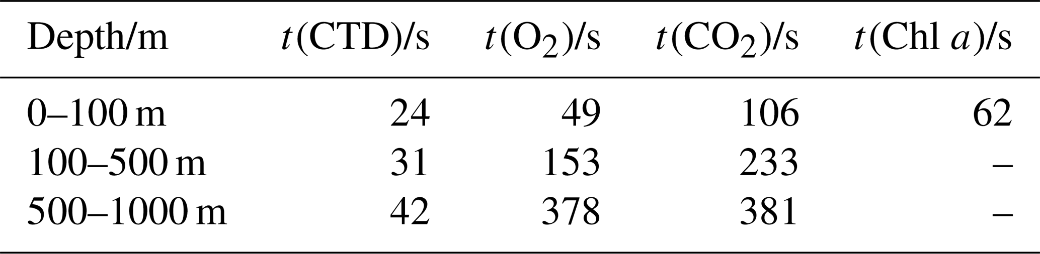
Kongsberg Seaglider 564 was deployed in the Norwegian Sea on 16 March 2014 at 63.00∘ N, 3.86∘ E, and recovered on 30 October 2014 at 62.99∘ N, 3.89∘ E. The Seaglider was equipped with a prototype Aanderaa 4797 CO2 optode, an Aanderaa 4330F oxygen optode (Tengberg et al., 2006), a Sea-Bird conductivity–temperature–depth profiler (CTD) and a combined backscatter–chlorophyll a fluorescence sensor (Wetlabs Eco Puck BB2FLVMT). The mean sampling intervals for each sensor varied with depth (Table 1).
Table 1Average sampling interval of Sea-Bird CTD, Aanderaa 4330F oxygen optode, Aanderaa 4797 CO2 optode and a combined backscatter/chlorophyll a fluorescence sensor (Wetlabs Eco Puck BB2FLVMT) in the top 100, from 100 to 500 and from 500 to 1000 m.
The deployment followed the Svinøy trench from the open sea towards the Norwegian coast. The glider covered a 536 km long transect eight times (four times in each direction) for a total of 703 dives (Fig. 1).
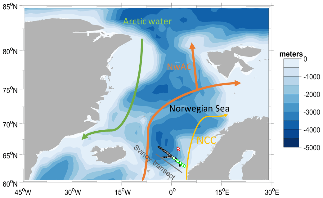
Figure 1Map of the glider deployment and the main currents. The black dots are the glider dives; the green and the red dots are the water samples collected along the glider section and at Ocean Weather Station M (OWSM), respectively. The three main water masses (Skjelvan et al., 2008) are the Norwegian Coastal Current (yellow), the Norwegian Atlantic Current (NwAC, orange) and Arctic Water (green).
2.2 Discrete sampling
During the glider deployment, 70 discrete water samples from various depths (5, 10, 20, 30, 50, 100, 300, 500 and 1000 m) were collected on five different cruises on the R/V Haakon Mosby along the southern half of the glider transect on 18 March, 5 May, 6 and 14 June, and 30 October 2014. Samples for c(DIC) and AT were collected from 10 L Niskin bottles following standard operational procedure (SOP) 1 of Dickson et al. (2007). The c(DIC) and AT samples were preserved with saturated HgCl2 solution (final HgCl2 concentration: 15 mg dm−3) and analysed within 14 d after the collection. Nutrient samples from the same Niskin bottles were preserved with chloroform (Hagebo and Rey, 1984). c(DIC) and AT were analysed on shore according to SOPs 2 and 3b (Dickson et al., 2007) using a VINDTA 3D (Marianda) with a CM5011 coulometer (UIC instruments) and a VINDTA 3S (Marianda), respectively. The precision of the samples' c(DIC) and AT values was 1 µmol kg−1 for both, based on duplicate samples and running Certified Reference Material (CRM) batch numbers 118 and 138 provided by professor A. Dickson, Scripps Institution of Oceanography, San Diego, USA (Dickson et al., 2003). Nutrients were analysed on shore using an Alpkem AutoAnalyzer. In addition, 43 water samples were collected at Ocean Weather Station M (OWSM) on five different cruises: 22 March on R/V Haakon Mosby, 9 May on R/V G.O. Sars, 14 June on R/V Haakon Mosby, 2 August and 13 November 2014 on R/V Johan Hjort from 10, 30, 50, 100, 200, 500, 800 and 1000 m depths. The OWSM samples were preserved and analysed for AT and c(DIC) as the Svinøy samples. No phosphate and silicate samples were collected at OWSM. Temperature (θ) and salinity (S) profiles were measured at each station using a Sea-Bird 911 plus CTD. pH and f(CO2) were calculated using the MATLAB toolbox CO2SYS (Van Heuven et al., 2011), with the following constants: K1 and K2 carbonic acid dissociation constants of Lueker et al. (2000), K(HSO/SO) bisulfate dissociation constant of Dickson (1990) and borate to chlorinity ratio of Lee et al. (2010). The precision of AT and c(DIC) led to an uncertainty in the calculated c(CO2) of 0.28 µmol kg−1. For the OWSM calculations, we used nutrient concentrations from the Svinøy section at a time as close as possible to the OWSM sampling as input. In the case of the glider, we derived a parameterisation for phosphate and silicate concentration as a function of sample depth and time. This parameterisation had an uncertainty of 1.3 and 0.13 µmol kg−1 and a R2 of 0.6 and 0.4, for silicate and phosphate concentrations, respectively. The uncertainty was calculated as the root mean square difference between measured and parameterised concentrations. This nutrient concentration uncertainty contributed an uncertainty of 0.04 µmol kg−1 in the calculation of c(CO2), which is negligible and smaller than the uncertainty caused by AT and c(DIC).
2.3 Oxygen optode calibration
The last oxygen optode calibration before the deployment was performed in 2012 as a two-point calibration at 9.91 ∘C in air-saturated water and at 20.37 ∘C in anoxic Na2SO3 solution. Oxygen optodes are known to be affected by drift (Bittig and Körtzinger, 2015), which is even worse for the fast-response foils used in the 4330F optode for glider deployments. It has been suggested that it is necessary to calibrate and drift correct the optode using discrete samples or in-air measurements (Nicholson and Feen, 2017). Unfortunately, no discrete samples were collected at glider deployment or recovery.
To overcome this problem, we used archived data to correct for oxygen optode drift. These archived concentration data (designated cC(O2)) were collected at OWSM between 2001 and 2007 (downloaded from ICES database) and in the glider deployment region between 2000 and 2018 (extracted from GLODAPv2; Olsen et al., 2016). To apply the correction, we used the oxygen samples corresponding to a potential density σ0 > 1028 kg m−3 (corresponding to depths between 427 and 1000 m), because waters of these potential densities were always well below the mixed layer and therefore subject to limited seasonal and interannual variability, as evidenced by the salinity S and potential temperature θ of these samples: S varied from 34.88 to 34.96, with a mean of 34.90 ± 0.01; θ varied from 0.45 to −0.76 ∘C, with a mean of (−0.15 ± 0.36) ∘C.
Figure 2 shows that the glider oxygen concentration (cG(O2)) corresponding to σ0 > 1028 kg m−3 was characterised by two different water masses separated at a latitude of about 64∘ N. We used the samples collected north of 64∘ N to derive the glider optode correction because this reflects the largest area covered by the glider. We did not use the southern region because the archived samples from there covered only 5 d. For each day of the year with archived samples, we calculated the median concentration of the glider and the archived samples. Figure 3 shows a plot of the ratio between against the day of the year and a linear fit, which is used to calibrate cG(O2) and correct for drift.
No lag correction was applied because the O2 optode had a fast response foil and showed no detectable lag (< 10 s), based on a comparison between descent and ascent profiles.
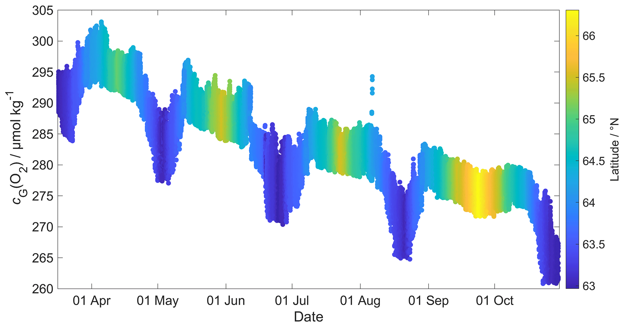

Figure 3A linear fit of the ratio between the daily median of the discrete oxygen samples (cC(O2)) and glider oxygen data (cG(O2)) for σ0 > 1028 kg m−3 was used to derive the cG(O2) drift and initial offset at deployment. The time difference Δt is calculated with respect to the deployment day on 16 March.
2.4 CO2 optode measurement principle
The CO2 optode consists of an optical and a temperature sensor incorporated into a pressure housing. The optical sensor has a sensing foil comprising two fluorescence indicators (luminophores), one of which is sensitive to pH changes, and the other is not and thus used as a reference. The excitation and emission spectra of the two fluorescence indicators overlap, but the reference indicator has a longer fluorescence lifetime than the pH indicator. These two fluorescence lifetimes are combined using an approach known as dual lifetime referencing (DLR) (Klimant et al., 2001; von Bültzingslöwen et al., 2002). From the phase shift (φ), the partial pressure of CO2, p(CO2), is parameterised as an eight-degree polynomial (Atamanchuk et al., 2014):
where C0 to C8 are temperature-dependent coefficients.
The partial pressure of CO2 is linked to the CO2 concentration, c(CO2) and the fugacity of CO2, f(CO2), via the following relationship:
where F(CO2) is the solubility function (Weiss and Price, 1980), p(H2O) is the water vapour pressure, p is the total gas tension (assumed to be near 1 atm), and K0(CO2) is the solubility coefficient. F and K0 vary according to temperature and salinity.
2.5 CO2 optode lag and drift correction and calibration
The CO2 optode was fully functional between dives 31 (on 21 March 2014) and 400 (on 24 July 2014). After dive 400, the CO2 optode stopped sampling in the top 150 m. Figure 4 shows the outcome of each calibration step: (0) uncalibrated optode output (blue dots), (1) drift correction (red dots), (2) lag correction (green dots) and (3) calibration using discrete water samples (black dots).
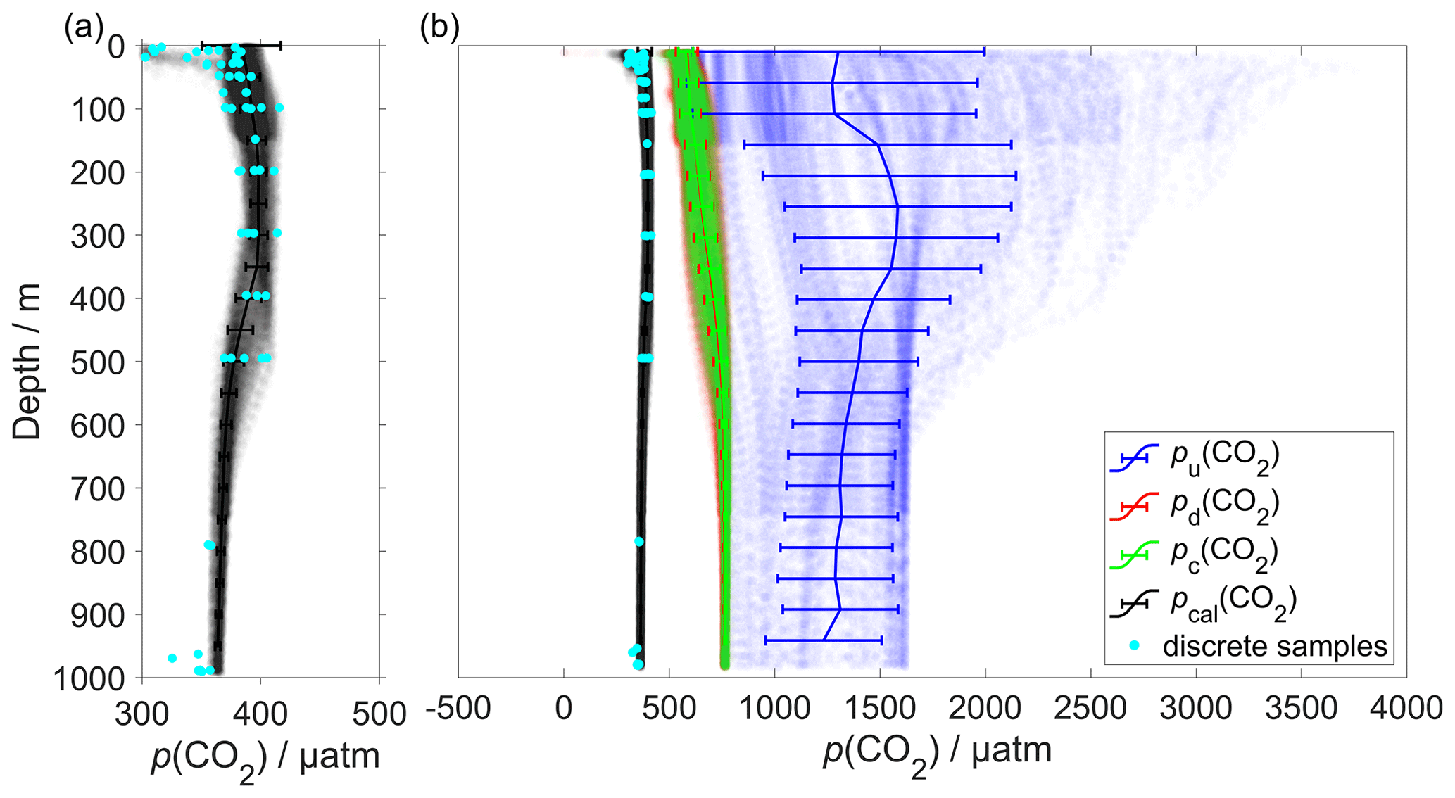
Figure 4Panel (a) shows the calibrated p(CO2) (pcal(CO2)) in black and the discrete samples in azure. (b) Plot of p(CO2) versus depth where the continuous vertical lines are the mean every 50 m and the error bars represent the standard deviation. Blue colour shows pu(CO2) without any correction; red shows pd(CO2) corrected for drift; green represents pc(CO2) corrected for drift and lag; black shows pcal(CO2) calibrated against water samples (azure dots) collected during the deployment (Sect. 2.5). pcal(CO2) had a mean standard deviation of 22 µatm and a mean bias of 1.8 µatm compared with the discrete samples.
In order to correct for the drift occurring during the glider mission, we selected the CO2 optode measurements in water with σ0>1028 kg m−3 (just as for O2; Sect. 2.3). We calculated the median of the raw optode phase shift data (“CalPhase” φcal) for each Seaglider dive. Then, we calculated a drift coefficient (mi) as the ratio between the median φcal for a given dive divided by the median φcal of dive 31. Drift-corrected φcal,d values were calculated by dividing the raw φcal by the specific mi for each dive.
The CO2 optode was also affected by lag (Atamanchuk et al., 2014) caused by the slow response of the optode to ambient c(CO2) changes in time and depth. The lag created a discrepancy between the depth profiles obtained during glider ascents and descents. To correct for this lag, we applied the method of Miloshevich (2004), which was previously used by Fiedler et al. (2013) and Atamanchuk et al. (2015b) to correct the lag of the Contros HydroC CO2 sensor (Fiedler et al., 2013; Saderne et al., 2013). This CO2 sensor has a different measurement principle (infrared absorption) than the CO2 optode, but both rely on the diffusion of CO2 through a gas-permeable membrane.
To apply the lag correction, the sampling interval (Δt) needs to be sufficiently small compared to the sensor response time (τ) and the ambient variability (Miloshevich, 2004). Before the lag correction, φcal,d was smoothed to remove any outliers and “kinks” in the profile using the Matlab function rLOWESS. The smoothing function applies a local regression every nine points using a weighted robust linear least-squares fit. Subsequently, τ was determined such that the following lag-correction equation (Miloshevich, 2004) minimised the φcal,d difference between each glider ascent and the following descent:
where pd(CO2,t0) is the drift-corrected value measured by the optode at time t0, pd(CO2,t1) is the measured value at time t1, Δt is the time between t0 and t1, τ is the response time, and pc(CO2,t1) is the lag-corrected value at t1. We calculated a τ value for each glider dive and used the median of τ (1384 s, 25th quartile: 1101 s; 75th quartile: 1799 s) (Fig. 5), which was larger than Δt(258 s) and therefore met the requirement to apply the Miloshevich (2004) method. To apply the lag correction, the glider needs to sample same water mass during the ascent and descent. The difference between the ascent and descent was minimal: it was (0.13 ± 0.33) ∘C for θ and 0.02 ± 0.04 for S. This lag correction reduced the average difference between glider ascent and descent from (71 ± 30) to (21 ± 26) µatm.

Figure 5The histogram shows the distribution of the τ calculated from glider dives 31 to 400 to correct the CO2 optode drift using the algorithm of Miloshevich (2004).
The CO2 optode output was calibrated using the discrete samples collected throughout the mission. Using the discrete sample time and potential density σ0, we selected the closest CO2 optode output. A linear regression between optode output and c(CO2) from the discrete samples (cWS(CO2) was used to calibrate the optode output pc(CO2) in terms of c(CO2). c(CO2) had a better correlation than p(CO2) (R2=0.77 vs. R2=0.02).
Plotting the regression residuals (cr(CO2), calculated as the difference between cWS(CO2) and the value predicted by the regression) revealed a quadratic relation between the regression residuals and water temperature (θ). We have therefore included θ and θ2 in the optode calibration (Fig. 6a). This second calibration increased the correlation coefficient R2 from 0.77 to 0.90 and decreased the standard deviation of the regression residuals from 1.3 to 0.8 µmol kg−1. Even with the explicit inclusion of temperature in the calibration, the CO2 optode response remained more closely related to c(CO2) than p(CO2) (Fig. 6b).
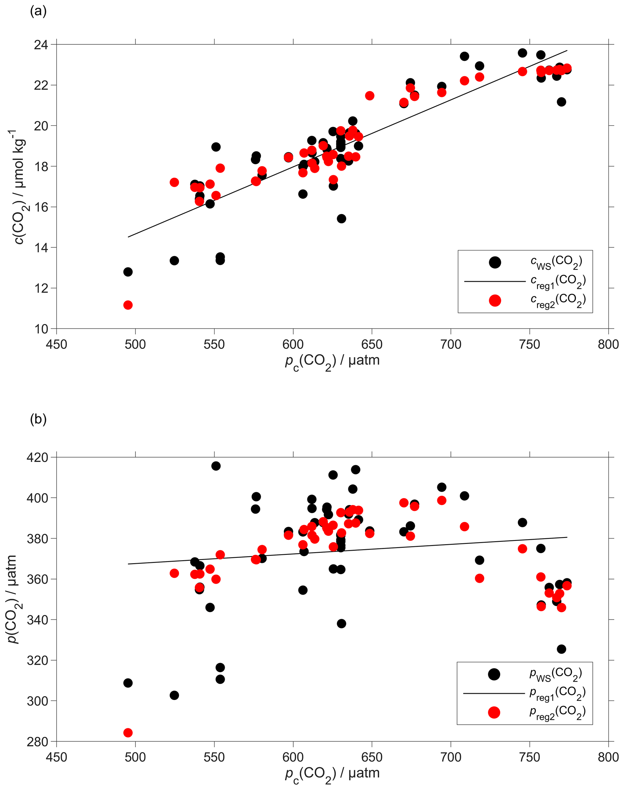
Figure 6Regression (black lines, reg1) of the CO2 optode output pc(CO2) against (a) co-located concentration cWS(CO2) that has an uncertainty of 0.28 µmol kg−1 (b) and partial pressure pWS(CO2) of CO2 in discrete water samples (black dots). Also shown are the values predicted by including θ and θ2 in the regression used for optode calibration (red dots, reg2). The regression equations are (a) reg1: cWS(CO2)/(µmol kg−1) = (0.033 ± 0.003)pc(CO2)/µatm – 1.8 ± 1.6 (R2=0.77); reg2: cWS(CO2)/(µmol kg−1) = (0.12 ± 0.14)θ/∘C – (0.071 ± 0.011)(θ/∘C)2 + (0.0094 ± 0.0048)pc(CO2)/µatm + 16 ± 4 (R2=0.90). (b) reg1: pWS(CO2)/µatm = (0.05 ± 0.05)pc(CO2)/µatm + 344 ± 33 (R2=0.02); reg2: pWS(CO2)/µatm = (21 ± 3)θ/∘C – (1.9 ± 0.2)(θ/∘C)2 + (0.2 ± 0.1)pc(CO2)/µatm + 209 ± 76 (R2=0.60).
2.6 Regional algorithm to estimate AT
To calculate c(DIC), we used two variables: (1) glider c(CO2) derived as described in Sect. 2.5 and (2) AT derived using a regional algorithm based on S and θ depths of less than 1000 m. The algorithm followed the approach of Lee et al. (2006) and was derived using 663 water samples collected at OWSM from 2004 to 2014 and GLODAPv2 (Olsen et al., 2016) data from the year 2000 in the deployment region. Discrete samples with S<33 were removed because these values were lower than the minimum S measured by the glider. The derived AT parameterisation is
The parameterisation has an uncertainty of 8.2 µmol kg−1 calculated as the standard deviation of the residual difference between actual and parameterised AT.
To test this parameterisation, we compared the predicted AT,reg values with discrete measurements (AT,WS) collected close in terms of time, potential density (σ0) and distance to the glider transect (n=60). These discrete samples and the glider had mean temperature and salinity differences of (0.17 ± 0.68) ∘C and 0.03 ± 0.013, respectively. The mean difference between AT,WS and AT,reg was (2.1 ± 6.5) µmol kg−1.
This AT parameterisation was used in CO2SYS (Van Heuven et al., 2011) to calculate c(DIC) from AT,reg and the calibrated c(CO2), cG,cal(CO2). These calculated cG,cal(DIC) values were compared with cWS(DIC) of the same set of discrete samples used to calibrate cG,cal(CO2), the only difference being that instead of the actual total alkalinity of the water sample (AT,WS), we used AT,reg. The mean difference between cG,cal(DIC) and cWS(DIC) was (3 ± 11) µmol kg−1, with the non-zero bias and the standard deviation due to the uncertainties in the AT,reg parameterisation and the cG,cal(CO2) calibration.
2.7 Quality control of other measurement variables
The thermal lag of the glider conductivity sensor was corrected using the method of Gourcuff (2014). Single-point outliers in conductivity were removed and replaced by linear interpolation. The glider CTD salinity was affected by presumed particulate matter stuck in the conductivity cell (Medeot et al., 2011) during dives 147, 234, 244, 251, 272, 279, 303, 320 and 397, and sensor malfunction caused a poor match between glider ascent and descent during dives 214, 215, 235 and 243. These dives were removed from the subsequent analysis.
Glider-reported chlorophyll concentrations, craw(Chl a), were computed using the factory coefficients. craw(Chl a) was affected by photochemical quenching during the daytime dives. To correct for quenching, we used the method of Hemsley et al. (2015) based on the nighttime relationship between fluorescence and optical backscatter. This relationship was established in the top 60 m and the nighttime values were selected between sunset and sunrise. We calculated a linear fit between craw(Chl a) measured at night, cN(Chl a), and the backscatter signal measured at night (bN). The slope and the intercept were then used to derive corrected daytime cD(Chl a). The glider-reported chlorophyll concentration has not been calibrated against in situ samples and is not expected to be accurate, even after correction for quenching. However, it should give an indication of the depth of the deep chlorophyll concentration maximum (zDCM) and the direction of chlorophyll concentration change (up/down). The 8 d means of craw(Chl a) were compared with satellite 8 d composite chlorophyll concentration (Fig. 7) from Ocean Colour CCI (https://esa-oceancolour-cci.org/, last access: 7 May 2020) and gave a mean difference of (0.12 ± 0.08) mg m−3.
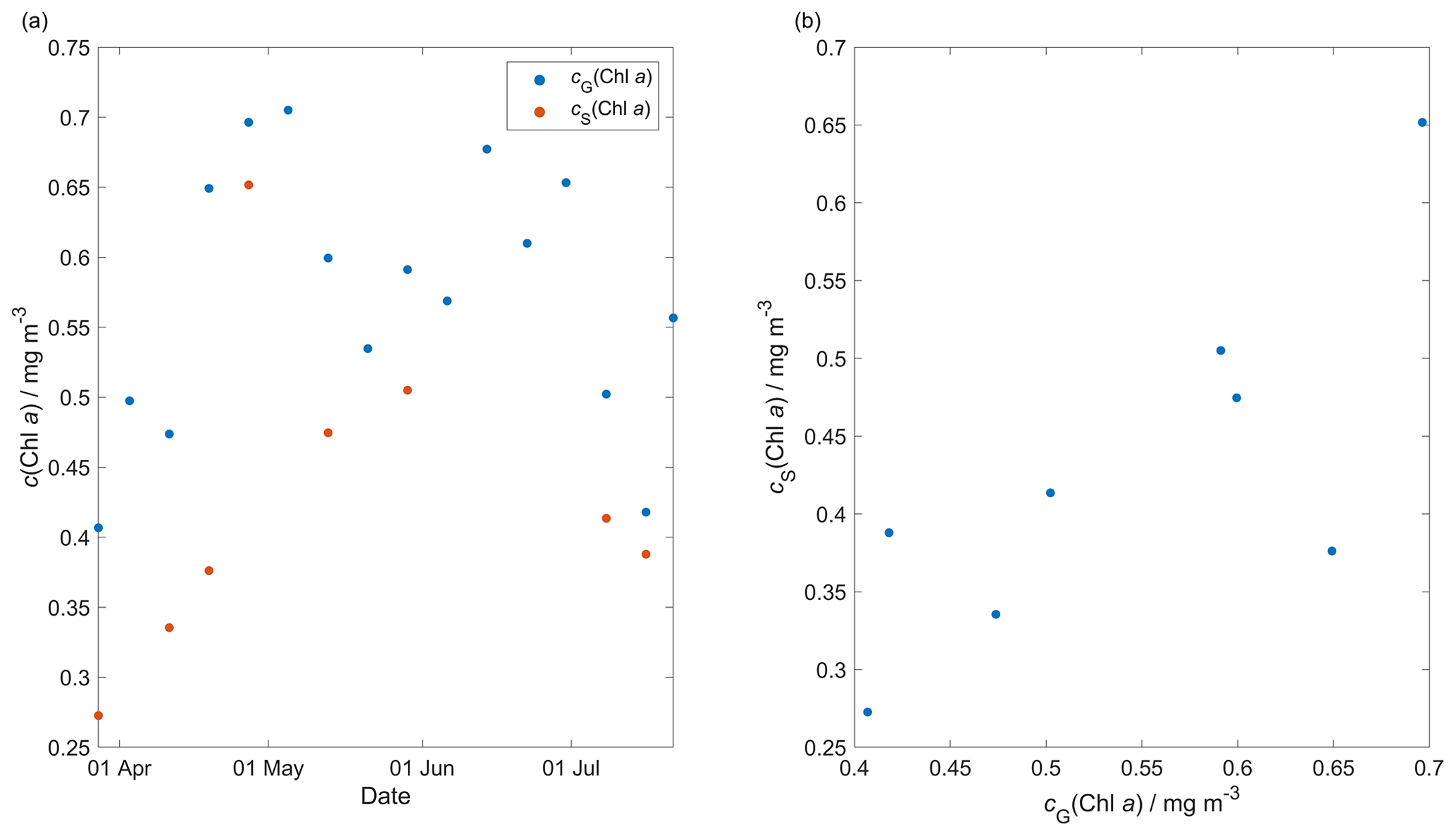
Figure 7Comparison between the 8 d glider c(Chl a) (cG(Chl a)) mean and the 8 d satellite c(Chl a) (cS(Chl a)) download from Ocean Colour CCI (https://esa-oceancolour-cci.org/, last access: 7 May 2020) as a time series (a) and scatter plot (b).
2.8 Calculation of oxygen-based net community production N(O2)
Calculating net community production N from glider data is challenging because the glider continuously moves through different water masses. For that reason, we subdivided the transect by binning the data into 0.1∘ latitude intervals to derive O2 concentration changes every two transects. The changes were calculated between transects in the same direction of glider travel (e.g. transects 1 and 3, both in the N–S direction) to have approximately the same time difference (40–58 d) at every latitude. If instead we had used two consecutive transects, this would lead to a highly variable time difference of near 0 to about 50 d along the transect.
We calculated N(O2) (in mmol m−2 d−1) from the oxygen inventory changes () corrected for air–sea exchange Φ(O2), normalised to zmix when zmix was deeper than the integration depth of zlim, entrainment E(O2) and diapycnal eddy diffusion Fv(O2):
The inventory changes were calculated as the difference between two transects of the integrated oxygen concentration C(O2). C(O2) (in mmol m−3) was derived from the oxygen content c(O2) (in µmol kg−1) by multiplication with the water density (about 1027 kg m−3, but we used the actual values). A default integration depth of 45 m was chosen to capture the deepest extent of the deep chlorophyll maximum (zDCM) found during the deployment, which likely represents the extent of the euphotic zone.
The inventory changes for every latitude bin were calculated using the following equation:
where n is the transect number, t is the day of the year, and C(O2,z) is the vertical O2 concentration profile.
The air–sea flux of oxygen, Φ(O2), was calculated for each glider dive using the median C(O2), θ and S in the top 10 m. We followed the method of Woolf and Thorpe (1991) that includes the effect of bubble equilibrium supersaturation in the calculations:
where kw(O2) is the gas transfer coefficient, Δbub(O2) is the increase of equilibrium saturation due to bubble injection, and Csat(O2) is the oxygen saturation. Csat(O2) was calculated from S and θ using the solubility coefficients of Benson and Krause (1984), as fitted by Garcia and Gordon (1992). Δbub(O2) was calculated from the following equation:
where U is 10 m wind speed with 1 h resolution (ECMWF ERA5; https://www.ecmwf.int/en/forecasts/datasets/reanalysis-datasets/era5, last access: 1 February 2021) and U0 represents the wind speed when the oxygen concentration is 1 % supersaturated and has a value of 9 m s−1 (Woolf and Thorpe, 1991). U has a spatial resolution of 0.25∘ latitude and 0.25∘ longitude and was interpolated to the glider position at the beginning of the dive.
The transfer velocity kw(O2) was calculated based on Wanninkhof (2014):
The Schmidt number, Sc(O2), was calculated using the parameterisation of Wanninkhof (2014). To account for wind speed variability, kw(O2) applied to calculate N(O2) was a weighted mean. This value was calculated using the varying daily-mean wind speed U in the time interval between tn and tn+1(Δt) (50 d) using a five-point-median zmix (Sect. 3.2) (Reuer et al., 2007). The time interval is the same as the one used to calculate .
The entrainment flux, E(O2), was calculated as the oxygen flux when the mixed layer depth deepens in time and is greater than zlim at time t2:
where t2−t1 represents the change in time, zmix is the mixed layer depth, I(O) is the expected inventory that would result from a mixed layer deepening to zmix(t2) between t2 and t1, and I(O) is the original inventory at t1.
The effect of diapycnal eddy diffusion (Fv) was calculated at zmix when it was deeper than zlim and at zlim when zmix was shallower than zlim, using the following equation:
for a vertical eddy diffusivity (Kz) of 10−5 m2 s−1 (Naveira Garabato et al., 2004). The effect of Fv(O2) on N(O2) was negligible (Fig. A2b) with a median of (−0.1 ± 0.5) mmol m−2 d−1.
2.9 Calculation of dissolved inorganic carbon-based net community production, N(DIC)
N(DIC) was expressed in mmol m−2 d−1 and was calculated from DIC inventory changes (), air–sea flux of CO2, Φ(CO2), entrainment E(DIC) and diapycnal diffusion Fv(DIC):
Firstly, Φ(CO2) was calculated using the 10 m wind speed with 1 h resolution downloaded from ECMWF ERA5. As for oxygen, we selected the closest wind speed data point at the beginning of each glider dive. We used the monthly mean atmospheric CO2 dry mole fraction (x(CO2)) downloaded from the Greenhouse Gases Reference Network Site (https://www.esrl.noaa.gov/gmd/ccgg/ggrn.php, last access: 28 February 2019) closest to the deployment at Mace Head, County Galway, Ireland (Dlugokencky et al., 2015). Using x(CO2), we calculated the air-saturation concentration Catm(CO2):
where pbaro is the mean sea level pressure and F(CO2) is the CO2 solubility function (in mol dm−3 atm−1) calculated from surface θ and S (Weiss and Price, 1980).
The seawater C(CO2) at the surface was calculated using the median in the top 10 m between the glider ascent and descent of the following dive C(CO2). From this, Φ(CO2) was calculated:
k(CO2) was calculated using the parameterisation of Wanninkhof (2014):
Sc(CO2) is the dimensionless Schmidt number at the seawater temperature (Wanninkhof, 2014). To account for wind speed variability, kw(CO2) applied to calculate N(DIC) was a weighted mean based on the varying daily-mean wind speed U in the time interval between tn and tn+1(Δt) used to calculate and for 40–50 d to calculate Φ(CO2) (Sect. 3.2) (Reuer et al., 2007).
The DIC inventory changes were calculated in the top 45 m with the following equation:
Just as for C(O2), C(DIC) (in mmol m−3) was derived from the DIC content c(DIC) (in µmol kg−1) by multiplication with the water density (about 1027 kg m−3, but we used the actual values).
The entrainment flux, E(DIC), was calculated as the DIC flux when the mixed layer depth deepens in time and is greater than zlim at time t2:
As for oxygen, the effect of diapycnal eddy diffusion (Fv) was calculated at zmix when it was deeper than zlim and at zlim when zmix was shallower than zlim, using the following equation:
for a Kz of 10−5 m2 s−1 (Naveira Garabato et al., 2004). The effect of Fv(DIC) was negligible (Fig. A2a) with a median of (0.1 ± 0.3) mmol m−2 d−1.
The contribution of horizontal advection to N(DIC) was considered minimal over the timescales where we calculated inventory changes because previous studies have shown that changes in C(DIC) during summer are mainly controlled by biology and air–sea interactions (Gislefoss et al., 1998). For that reason, previous studies that estimated N in the Norwegian Sea have also neglected advective fluxes (Falck and Anderson, 2005; Falck and Gade, 1999; Kivimäe, 2007; Skjelvan et al., 2001).
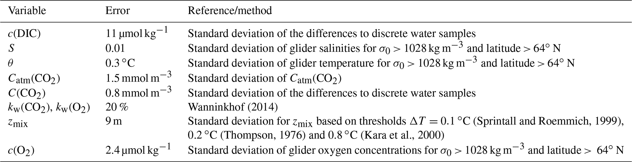
Uncertainties in N(DIC) and N(O2) were evaluated with a Monte Carlo approach. The uncertainties of the input variables are shown in Table 2; we repeated the analysis 1000 times. The total uncertainty in N was calculated as the standard deviation of the 1000 Monte Carlo simulations.
Table 2Uncertainty associated with N(DIC) and N(O2) input variables calculated by a Monte Carlo approach.
The uncorrected p(CO2) values presented in Fig. 8 were analysed up to dive 400 (24 July 2014). For the following dives, the CO2 optode stopped sampling in the first 150 m (Fig. 8d). Instead, the uncorrected temperature θ, salinity S, c(O2) and craw(Chl a) were analysed for all the dives (30 October 2014). The raw optode c(O2) data were calibrated and drift corrected, and c(CO2) was drift corrected, lag corrected and recalibrated, then used to quantify the temporal and spatial changes in N and Φ together with the quenching corrected craw(Chl a) to evaluate net community production changes.
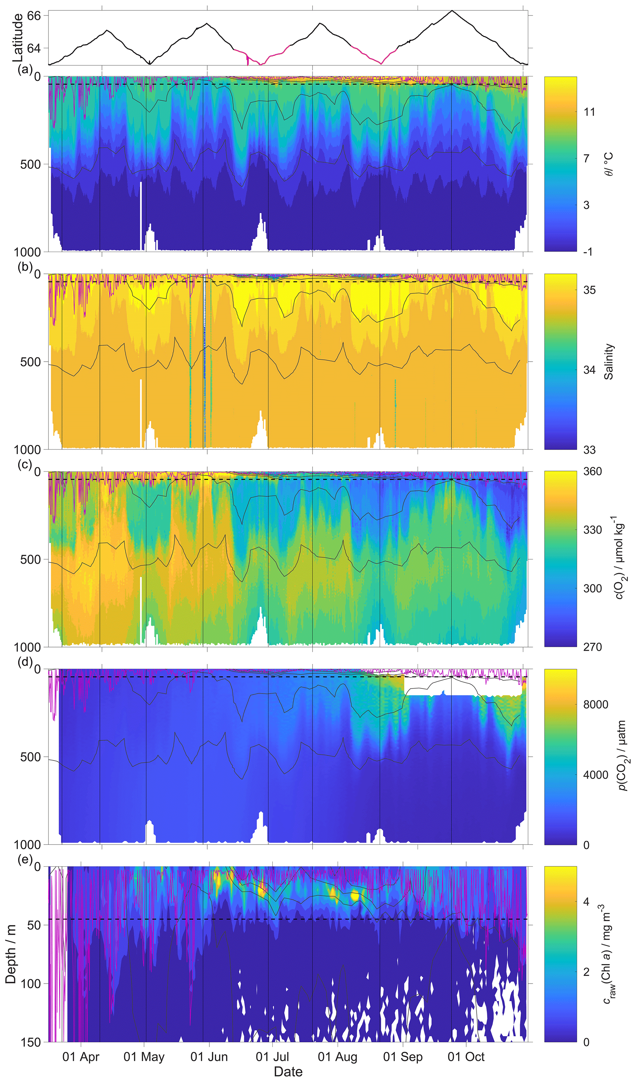
Figure 8Raw glider data for all 703 dives with latitude of the glider trajectory at the top (black: NwAC; red: NCC, separated by a S of 35). (a) Temperature θ, (b) salinity S, (c) oxygen concentration cG(O2), (d) uncorrected CO2 optode output pu(CO2) and (e) chlorophyll a concentration craw(Chl a). The white space means that the sensors did not measure any data. The pink line is zmix calculated using a threshold criterion of Δθ=0.5 ∘C to the median θ in the top 5 m (Obata et al., 1996; Monterey and Levitus, 1997; Foltz et al., 2003). The dotted black line designates zlim, used as a depth limit to calculate N. Contoured black lines represent isopycnals.
3.1 O2 and CO2 optode calibration
The O2 optode drift caused a continuous and unexpected decrease of the uncorrected cG(O2) from 290 to 282 µmol kg−1 for σ0 > 1028 kg m−3 (Fig. 8c). The ratio against day of the year used for the drift correction had a good correlation with time (R2=0.90), showing a continuous increase of 0.0004 d−1 (Fig. 3), equivalent to a decrease in the measured glider O2 concentration of 0.11 µmol kg−1 d−1. It was possible to apply the correction because cC(O2) had low temporal variability for the chosen potential density σ0 > 1028 kg m−3. The cC(O2) values from OWSM and GLODAPv2 had a mean of (305 ± 3) µmol kg−1, varying from 294 to 315 µmol kg−1 (Fig. A1). The drift correction reduced the variability of cG(O2) in the selected potential density range from a standard deviation of 7.3 µmol kg−1 to a standard deviation of 2.4 µmol kg−1 (Fig. 9a).

Figure 9(a) c(O2); (b) s(O2) = with zDCM (red line), zmix (pink line) five-point median zmix (dotted pink line). The black line indicates σ0=1028 kg m−3. The top panel indicates glider latitude (black: NwAC; red: NCC).
Following drift, lag and scale corrections, glider fugacity fG(CO2) derived from Eq. (2) had a mean difference of (2 ± 22) µatm to the discrete samples (n=55; not shown) and c(DIC) had a mean difference of (3 ± 11) µmol kg−1 (Fig. 10). p(CO2) and f(CO2) are almost identical, but f(CO2) takes into account the non-ideal nature of the gas phase. The optode was able to capture the temporal and spatial variability showing that NCC had a lower DIC concentration than NwAC. Restricting the f(CO2) comparison to the discrete samples in the top 10 m gave a mean difference of (19 ± 31) µatm (n=6). We also compared glider fG(CO2) with the Surface Ocean CO2 Atlas (SOCAT) f(CO2) (Bakker et al., 2016) data in the region during the deployment (Fig. 11). During the whole deployment, there was general agreement between fG(CO2) and fSOCAT(CO2). fG(CO2) varied between 204 and 391 µatm, while fSOCAT(CO2) varied between 202 and 428 µatm (Fig. 11).
Our results are in agreement with Jeansson et al. (2011), who found the surface NCC was the region with the lowest c(DIC) values (2083 µmol kg−1) in the Norwegian Sea. This was confirmed during our deployment because c(DIC) was (2081 ± 39) µmol kg−1 in the NCC region and (2146 ± 27) µmol kg−1 in the NwAC region (Fig. 10) and c(O2) was > 300 µmol kg−1 in the NwAC and < 280 µmol kg−1 in the NCC.
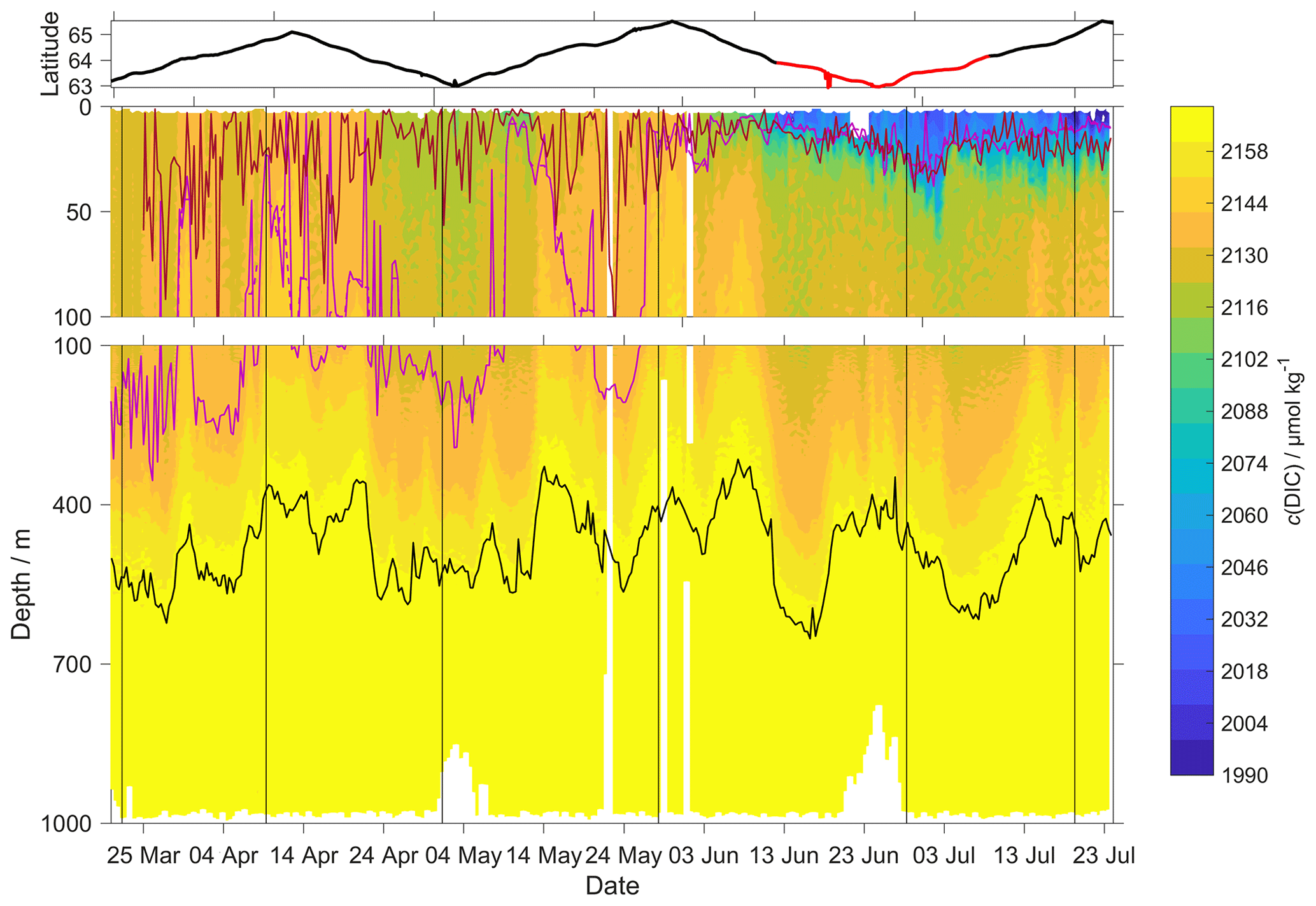
Figure 10c(DIC) contour plot with zDCM (red line), zmix (pink line) five-point median zmix (dotted pink line). The black line indicates σ0 = 1028 kg m−3. The top panel indicates glider latitude (black: NwAC; red: NCC).
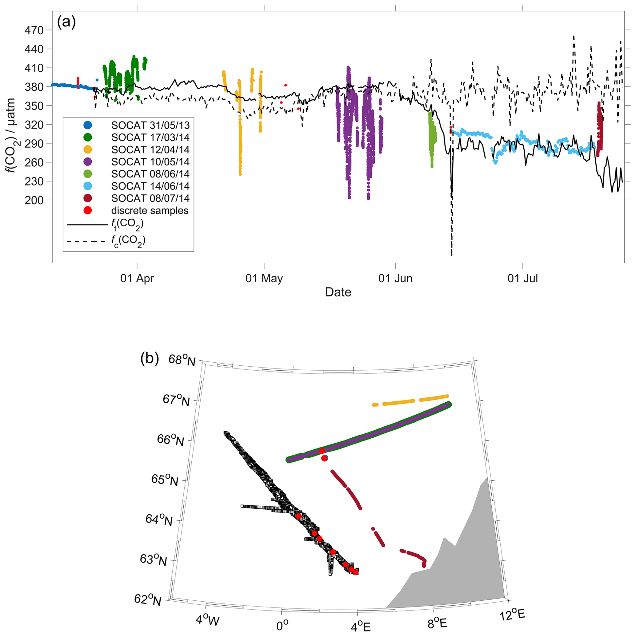
Figure 11Comparison between surface f(CO2) from 2014 SOCAT and CO2 optode on the glider. (a) The black lines are the median glider f(CO2) in the top 10 m, with fc(CO2) (dotted line) corresponding to regression 1 (Fig. 6a) and ft(CO2) (continuous line) to regression 2 (Fig. 6a). Discrete samples collected during the deployment are shown as red dots, with the other coloured dots representing cruises in the SOCAT database (Bakker et al., 2016). (b) Glider and SOCAT data positions (same colours as in panel a).
3.2 Air–sea exchange
The surface water was supersaturated with oxygen all summer (Fig. 12). From May, this supersaturation drove a continuous O2 flux from the sea to the atmosphere. However, the flux varied throughout the deployment, having a median of 25 mmol m−2 d−1 (5th percentile: −31 mmol m−2 d−1; 95th percentile: 88 mmol m−2 d−1). Prior to the spring period of increased Chl a inventory, the supersaturation varied between 0 to 10 µmol kg−1. Φ(O2) had a median of −1.4 mmol m−2 d−1 (5th percentile: −49 mmol m−2 d−1; 95th percentile: 23 mmol m−2 d−1). Then, during the spring period of increased Chl a inventory, the surface concentration increased by over 35 µmol kg−1, causing a peak in Φ(O2) of 140 mmol m−2 d−1. A second period of increased Chl a inventory was encountered in June and had a larger Φ(O2) up to 118 mmol m−2 d−1, driven by supersaturation of 68 µmol kg−1. The fluxes were smaller than during spring and were associated with an increase of craw(Chl a) from 2.5 mg m−3 to the summer maximum of 4.0 mg m−3. However, prior to the increased spring Chl a inventory, Φ(O2) showed a few days of influx into seawater caused by a decrease of θ from 7.6 to 5.9 ∘C that increased Csat(O2). The influx at the beginning of the deployment is partly due to the Δbub(O2) correction that resulted in for U > 10 m s−1. In August, the surface supersaturation decreased to 2.3 µmol kg−1 and Φ(O2) decreased to a monthly minimum of −7.6 mmol m−2 d−1. In the second half of September, the surface water became undersaturated by −2.6 µmol kg−1, causing O2 uptake with a median flux of −13 mmol m−2 d−1 (5th percentile: −39 mmol m−2 d−1; 95th percentile: 10 mmol m−2 d−1).
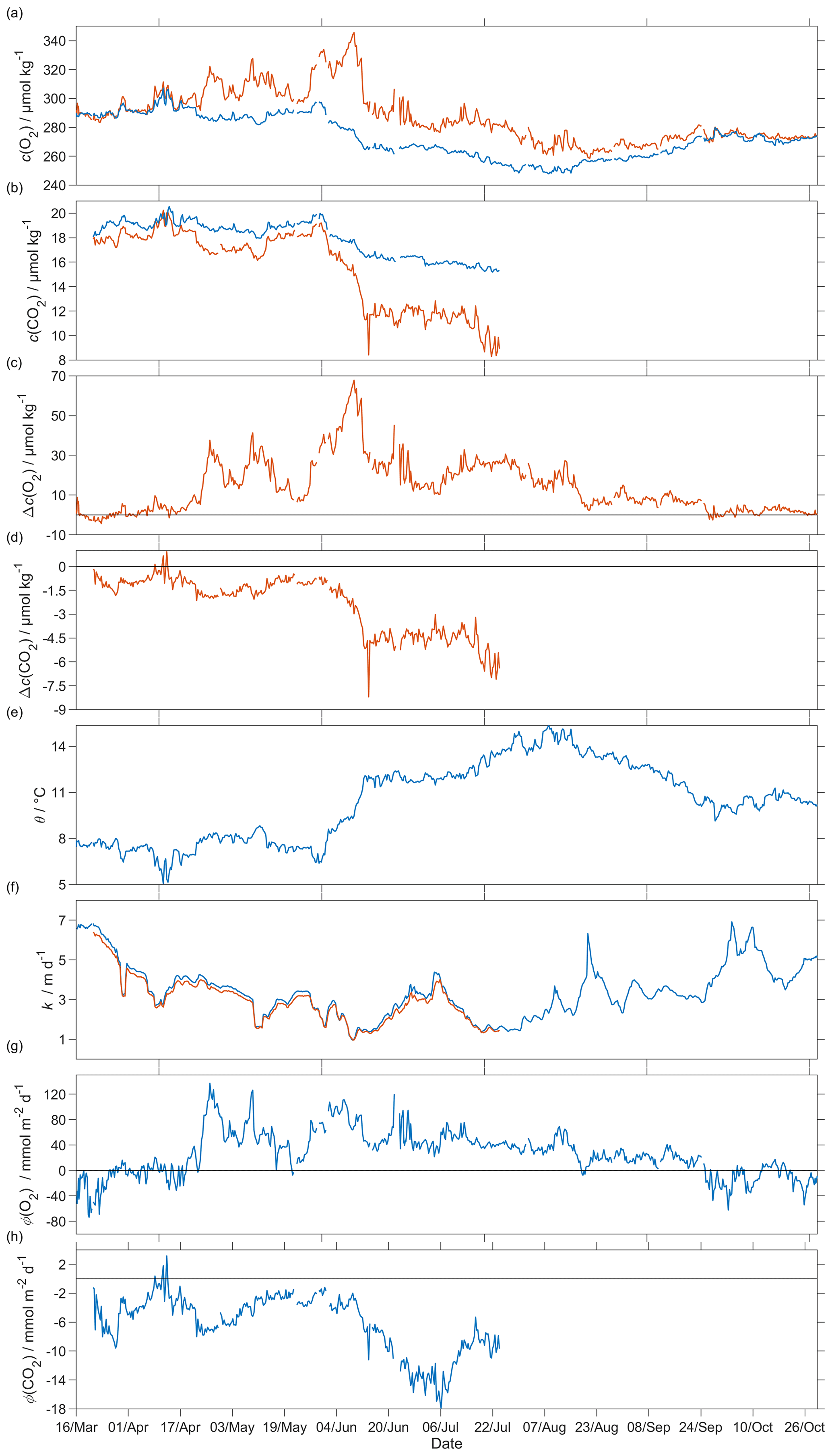
Figure 12Air–sea flux of O2 and CO2 during spring and summer for CO2 and during spring, summer and autumn for O2, (a) csat(O2) in blue and c(O2) in red, (b) csat(CO2) in blue and c(CO2) in red, (c) Δc(O2) = c(O2)−csat(O2), (d) Δc(CO2) = c(CO2)−csat(CO2), (e) sea surface temperature, (f) kw(O2) in blue and kw(CO2) in red normalised back to 50 d (Reuer et al., 2007), (g) oxygen air–sea flux Φ(O2) and (h) CO2 air–sea flux Φ(CO2). The flux from sea to air is positive, while that from air to sea is negative.
The CO2 flux from March to July was always from the air to the sea (Fig. 12), with a median of −5.2 mmol m−2 d−1 (5th percentile: −14 mmol m−2 d−1; 95th percentile: −1.5 mmol m−2 d−1). An opposite flux direction is expected for Φ(O2) and Φ(CO2) during the productive season when net community production is the main driver of concentration changes. After the summer period of increased Chl a inventory, the flux had a median of −11 mmol m−2 d−1 (5th percentile: −16 mmol m−2 d−1; 95th percentile: −6.8 mmol m−2 d−1), in agreement with previous studies that classified the Norwegian Sea as a CO2 sink (Takahashi et al., 2002; Skjelvan et al., 2005). Φ(CO2) for the discrete samples from 18 March to 14 June (n=13) varied from 0.1 to −13 mmol m−2 d−1.
3.3 N(O2)
To capture the entire euphotic zone, we calculated N(O2) and N(DIC) using an integration depth of zlim=45 m because the mean deep chlorophyll maximum (DCM) depth was zDCM = (20 ± 18 m) (Fig. 9). For comparison, the mixed layer depth was deeper, varied more strongly and had a mean value of zmix = (68 ± 78) m, using a threshold criterion of Δθ=0.5 ∘C to the median θ value in the top 5 m of the glider profile (Obata et al., 1996; Monterey and Levitus, 1997; Foltz et al., 2003).
The two N values were calculated as the difference in inventory changes between two transects when the glider moved in the same direction.
During the deployment, we sampled two periods of increased Chl a inventory, the first one in May and a second one in June. The chlorophyll a inventory () was calculated integrating craw(Chl a) to zlim. To remove outliers, we used a five-point moving mean of .
The N(O2) changes were dominated by Φ(O2), which had an absolute median of 34 mmol m−2 d−1 (5th percentile: 4.3 mmol m−2 d−1; 95th percentile: 86 mmol m−2 d−1), followed by I(O2), which had a median of 15 mmol m−2 d−1 (5th percentile: 2.3 mmol m−2 d−1; 95th percentile: 29 mmol m−2 d−1), Fv(O2), which had an absolute median of 0.3 mmol m−2 d−1 (5th percentile: 0 mmol m−2 d−1; 95th percentile: 1.0 mmol m−2 d−1) and E(O2), which had a median of 0 mmol m−2 d−1 (5th percentile: −1.2 mmol m−2 d−1; 95th percentile: 0 mmol m−2 d−1).
At the beginning of May, increased to 97 mg m−2 and N(O2) = (95 ± 16) mmol m−2 d−1. After this period, decreased to 49 mg m−2 and N(O2) = (−4.6 ± 1.6) mmol m−2 d−1. During the summer increased to 110 mg m−2, which caused a sharp increase of N(O2) to (126 ± 25) mmol m−2 d−1. remained higher than 50 mg m−2 until the end of June when N(O2) was (31 ± 9) mmol m−2 d−1. The passage of the glider from NwAC to NCC was accompanied by a drop of surface c(O2) from 330 to 280 µmol kg−1 (Fig. 9) that resulted in lower Φ(O2) and N(O2) values (Fig. 13). At the same time, decreased to 35 mg m−2 showing that the decrease of N(O2) depended on the passage to NCC and a decrease of biological production. After the beginning of August, decreased to 49 mg m−2 and N(O2) turned negative with a minimum of (−23 ± 25) mmol m−2 d−1. In October, during the last glider transect, continued decreasing to 27 mg m−2 leading to the minimum N(O2) of (−52 ± 11) mmol m−2 d−1.
Integrating N(O2) from March to October gives a flux of 4.9 mol m−2 a−1 (Table 3; discussed in Sect. 4.2).
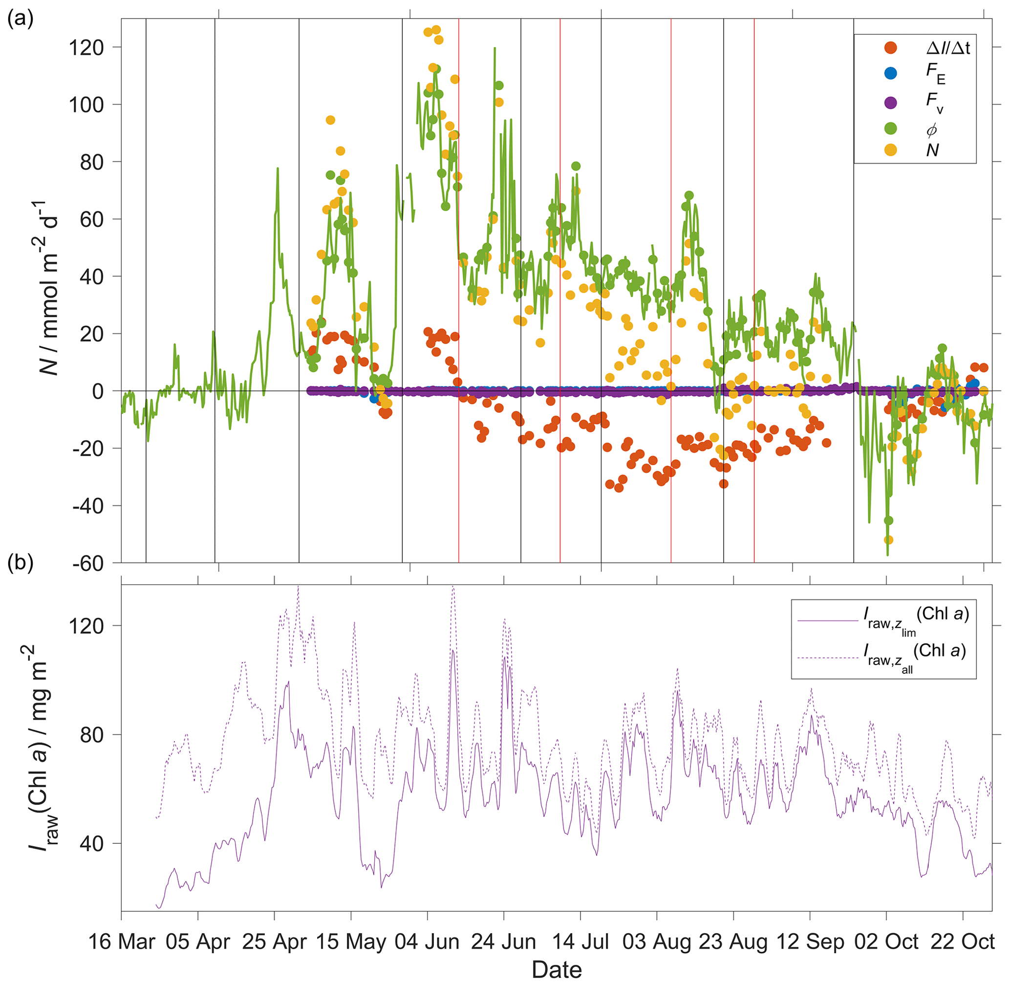
Figure 13(a) Components of the N(O2) calculation: (red), E(O2) (blue), Fv(O2) (violet), Φ(O2) (green) with kw(O2) weighted over 50 d, N(O2) (yellow). (b) Chl a inventory in the top 45 m, (violet). Chl a inventory for the whole water column, (dotted violet line). The vertical black lines represent each glider transect. Between the two vertical red lines, the glider was in the NCC region.
3.4 N(DIC)
In the case of N(DIC), the main drivers were the inventory changes with an absolute median of 29 mmol m−2 d−1 (5th percentile: 1.3 mmol m−2 d−1; 95th percentile: 57 mmol m−2 d−1), followed by Φ(CO2), which had an absolute median of 7.0 mmol m−2 d−1 (5th percentile: 0.8 mmol m−2 d−1; 95th percentile: 15 mmol m−2 d−1), Fv(DIC), which had an absolute median of 0.2 mmol m−2 d−1 (5th percentile: 0 mmol m−2 d−1; 95th percentile: 1.3 mmol m−2 d−1) and E(DIC), which had a median of 0 mmol m−2 d−1 (5th percentile: 0 mmol m−2 d−1; 95th percentile: 3.4 mmol m−2 d−1). During the period of increased Chl a inventory N(DIC) was (21 ± 4.5) mmol m−2 d−1. Later, decreased to 30 mg m−2 driving N(DIC) to negative values with a minimum of (−2.7 ± 5.0) mmol m−2 d−1. In the next transect, the glider measured the maximum of 111 mg m−2 that increased N(DIC) to (85 ± 4.5) mmol m−2 d−1. This maximum was reached during a transect when the glider moved in NCC, which had a c(DIC) of 2080 µmol kg−1 at the surface compared with the 2150 µmol kg−1 in NwAC and drove a continuous positive N(DIC), which had a minimum of (36 ± 7.4) mmol m−2 d−1 (Fig. 14).
Integrating N(DIC) from March to July gives a flux of 3.3 mol m−2 a−1 (Table 3; discussed in Sect. 4.2).
Table 3Net community production (N) estimates in the Norwegian Sea (with integration depth zlim). Falck and Anderson (2005) used year-round data from 1960 to 2000 between 62 and 70∘ N and from 1991 to 1994 at OWSM. Skjelvan et al. (2001) used year-round data from 1957 to 1970 and from 1991 to 1998 between 67.5∘ N, 9∘ E, and 71.5∘ N, 1∘ E, and along 74.5∘ N from 7 to 15∘ E. Kivimäe (2007) used year-round data from 1955 to 2005, and Falck and Gade (1999) used year-round data from 1955 to 1988 in all of the Norwegian Sea. While the previous studies report annual N estimates, the present study derives N(O2) between March and October and N(DIC) between March and July.

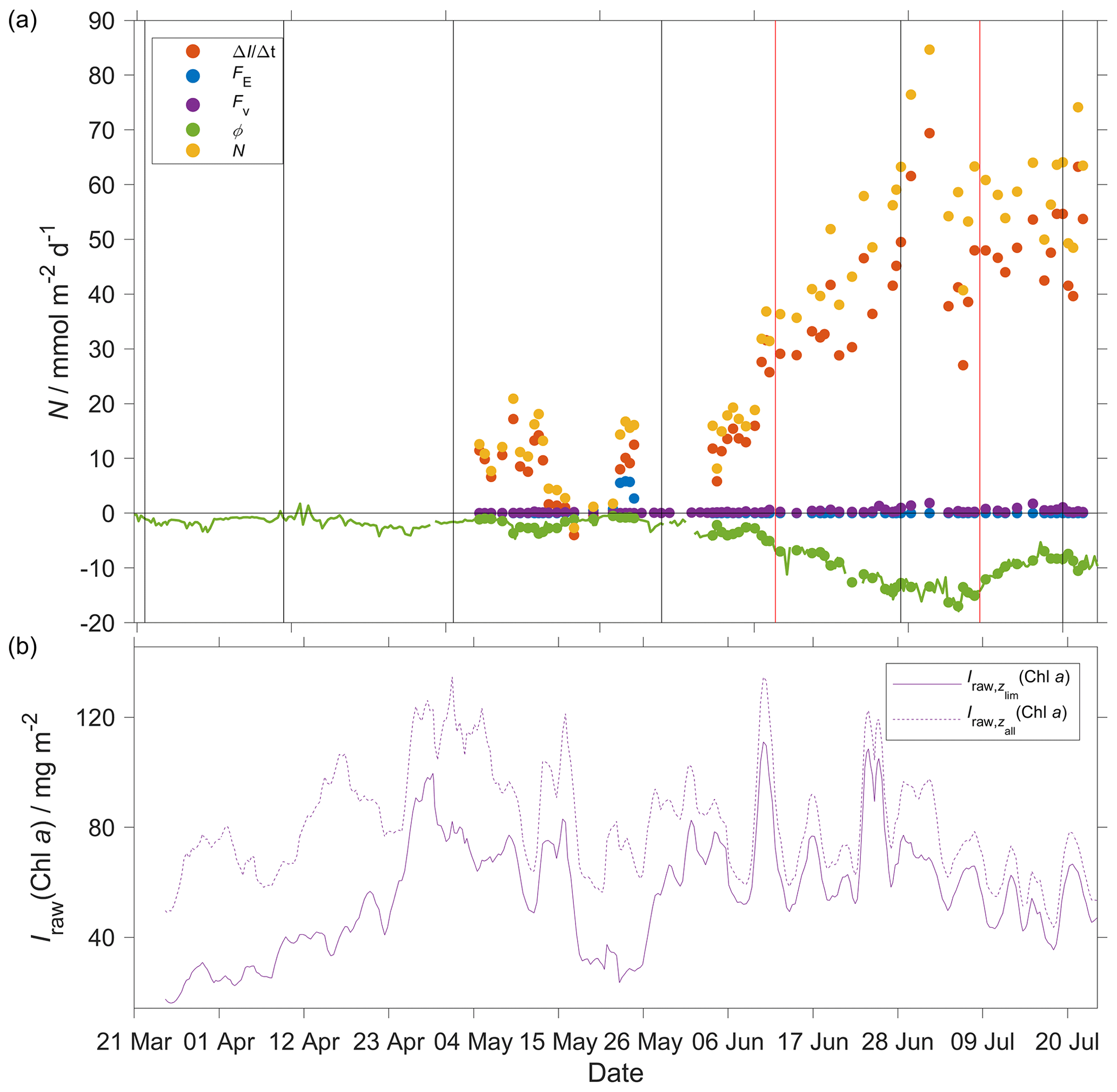
Figure 14(a) Components of the N(DIC) calculation: (red), E(DIC) (blue), Fv(CO2) (violet), Φ(CO2) (green) with kw(CO2) weighted over 50 d, N(DIC) (yellow). (b) Chl a inventory in the top 45 m, (violet). Chl a inventory for the whole water column, (dotted violet line). The vertical black lines represent each glider transect. Between the two vertical red lines, the glider was in the NCC region.
4.1 Sensor performance
This study presents data from the first glider deployment with a CO2 optode. The initial uncalibrated pu(CO2) measured by the CO2 optode had a median of 604 µatm (5th percentile: 566 µatm; 95th percentile: 768 µatm), whereas the p(CO2) of discrete samples varied from 302 to 421 µatm.
We applied corrections for drift (using deep-water samples as a reference point), sensor lag and calibrated the CO2 optode against co-located discrete samples throughout the water column.
Atamanchuk et al. (2014) reported that the sensor was affected by a lag that varied from 45 to 264 s depending on temperature. These values were determined in an actively stirred beaker. However, in this study, the sensor was mounted on a glider and was not actively pumped, which increased the response time to 23 min (25th quartile: 18 min; 75th quartile: 30 min). Also, the optode was affected by a continuous drift from 637 to 5500 µatm that was larger than the drift found by Atamanchuk et al. (2015a) which increased by 75 µatm after 7 months.
In this study, the drift- and lag-corrected sensor output showed a better correlation with the CO2 concentration c(CO2) than with p(CO2). The latter two quantities are related to each other by the solubility that varies with θ and S (Weiss, 1974) (Eq. 2). The better correlation with c(CO2) was probably related to an inadequate temperature parameterisation of the sensor calibration function. Including both temperature and temperature squared in the calibration gave a better fit with c(CO2) than with p(CO2) but overall still a lower calibration residual for the former. The sensor output depends on the changes in pH that are directly related to the changes of c(CO2) in the membrane and – indirectly – p(CO2), via Henry's law. The calibration is supposed to correct for the temperature dependence of the sensor output (Atamanchuk et al., 2014). So the fact that the sensor output correlated better with c(CO2) than p(CO2) is perhaps due to a fortuitous cancellation of an inadequate temperature parameterisation and Henry's law relationship between c(CO2) and p(CO2).
The calibrated optode output captured the c(DIC) changes in space and time with a standard deviation of 11 µmol kg−1 compared with the discrete samples. c(DIC) decreased from 2130 to 2000 µmol kg−1 and increased with depth to 2170 µmol kg−1. This shows the potential of the sensor for future studies that aim to analyse the carbon cycle using a high-resolution dataset.
The optode-derived CO2 fugacity fG(CO2) had a mean bias of (1.8 ± 22) µatm compared with the discrete samples. These values are comparable with a previous study when the CO2 optode was tested for 65 d on a wave-powered profiling cRAWLER (PRAWLER) from 3 to 80 m (Chu et al., 2020), which had an uncertainty between 35 and 72 µatm. The PRAWLER optode was affected by a continuous drift of 5.5 µatm d−1 corrected using a regional empirical algorithm that uses c(O2), θ, S and σo to estimate AT and c(DIC).
4.2 Norwegian Sea net community production
Increases in N(O2) and N(DIC) were associated with increases in depth-integrated craw(Chl a), designated as periods of increased Chl a inventory Iraw(Chl a), at the beginning of May and in June. During May, Iraw(Chl a) reached 135 mg m−2. In June, Iraw(Chl a) reached again 135 mg m−2. Between these two periods, N(DIC) briefly turned negative, indicating remineralisation of the high Chl a inventory material during this period. The period of increased Chl a inventory coincided with a surface temperature increase from 7 to 11 ∘C and shoaling of the mixed layer from 200 to 20 m. c(O2) reached a summer maximum of 340 µmol kg−1 and c(DIC) decreased to a summer minimum of 1990 µmol kg−1. In both cases, the main components of the N changes were the inventory and air–sea flux, while the smallest driver was the entrainment. Also, the glider sampled two different water masses characterised by different c(DIC) and c(O2). This might be the cause of the smaller values N(O2) and higher values N(DIC) in June and July in NCC compared to NwAC (Figs. 13 and 14). Another explanation might be a consumption of O2 due to remineralisation and a delay in the response of the c(DIC) that was lowered during the two blooms. A fully functional CO2 optode in the second part of the deployment would have helped to uncover the cause of the higher N(DIC) than of N(O2).
Table 3 shows estimates of net community production (N) in the Norwegian Sea. All other studies used ships to gather observations. The estimated N in the four other studies varied from 2.6 to 11.1 mol m−2 a−1 for N(O2) and was 3.4 for N(DIC). In our glider study, we obtained between March and July a N(DIC) of 3.3 mol m−2 a−1 and a N(O2) of 4.2 mol m−2 a−1, in agreement with these studies. The ratio of N(O2) and N(DIC) for an integration depth of 45 m gave a photosynthetic quotient (PQ) of 1.3, in agreement with the Redfield ratio of 1.45 ± 0.15 (Redfield, 1963; Anderson, 1995; Anderson and Sarmiento, 1994; Laws, 1991). The N(O2) estimate is influenced primarily by the air–sea exchange flux Φ(O2) (median: 34 mmol m−2 d−1), followed by the inventory change (15 mmol m−2 d−1). In contrast, N(DIC) is dominated by the inventory change (−29 mmol m−2 d−1), followed by Φ(CO2) (−7.0 mmol m−2 d−1). This reflects the slower gas-exchange time constant of CO2 compared with O2, due to DIC buffering. To compare our results with previous studies, we also used zlim=30 m (Falck and Gade, 1999) and 100 m (Falck and Anderson, 2005; Kivimäe, 2007). The calculated N(DIC; 30 m) was 3.1 mol m−2 a−1, N(DIC; 100 m) was 3.4 mol m−2 a−1, N(O2; 30 m) was 4.1 mol m−2 a−1 and N(O2; 100 m) was 3.7 mol m−2 a−1. The N(DIC; 100 m) value is in agreement with the value of 3.4 mol m−2 a−1 given by Falck and Anderson (2005). However, the latter estimate was for the entire year, whereas our estimate only covers the months from March to July. N(O2) was similar for zlim=30 and 45 m but lower for zlim=100 m because of O2 consumption during organic matter remineralisation below the euphotic zone. The PQ value at 30 was 1.3 and at 100 m decreased to 1.1. Extending N(O2) to October increased N(O2; 30 m) and N(O2; 45 m) to 5.0 and 4.9 mol m−2 a−1, respectively. Instead, N(O2; 100 m) decreased to 3.6 mol m−2 a−1, confirming the consumption of O2 below the euphotic zone. The calculated N(O2) until October was in agreement with the previous studies that varied between 2.6 and 11 mol m−2 a−1.
Some of the previous N(DIC) estimates derived c(DIC) from other variables such as c(O2), c(PO), c(NO), assuming Redfield ratios P : N : C : O2 1 : 16 : 106 : −138 (Redfield, 1963). During photosynthesis c(PO) and c(NO) are taken up by phytoplankton to form organic matter and are released again after remineralisation of the organic matter giving an indication of NCP changes. Our N(DIC) estimate was 3.3 mol m−2 a−1 and is similar to 3.4 mol m−2 a−1 estimated by Falck and Anderson (2005) who used c(DIC) samples directly. The carbon nutrient ratios vary between water masses and during photosynthesis (Thomas et al., 1999; Copin-Montégut, 2000; Osterroht and Thomas, 2000; Körtzinger et al., 2001).
The difference of the annual N(O2) and N(DIC) with the previous studies can also be caused by the yearly variability of N in the Norwegian Sea. In fact, Kivimäe (2007) saw an annual variability of N(O2) from 1955 to 2005 between 4.7 and 18.3 mol m−2 a−1. In order to understand what is causing these interannual changes, it is important capture inventory and air–sea changes. Also, this study showed that the Norwegian Sea spring, summer and autumn N is strongly affected by the time of sampling. For that reason, N estimated from low-resolution datasets makes the result strongly dependent on the time of sampling. To quantify this interannual variability in N, more high-resolution studies are needed.
To the best of our knowledge, this study represents the first glider deployment of a CO2 optode. The CO2 optode together with a O2 optode shows the potential of using these sensors on autonomous observing platforms like Seagliders to quantify the interactions between biogeochemical processes and the marine carbonate system at high spatiotemporal resolution. The deployment helped to uncover NCP and air–sea flux variability over a period of 8 months.
Despite all the problems (drift, lag and poor calibration), the CO2 optode data could be used to quantify dissolved inorganic carbon concentration variations. The temporal sampling resolution was 106 s in the top 100 m (increasing to 381 s from 500 to 1000 m). This could be improved to less than 10 s, but this would reduce the length of the deployment due to the limited glider battery capacity. With better calibration and stability improvements, the CO2 optode could be routinely used to measure the carbonate system on gliders, floats and surface vehicles. Glider deployments up to 8 months are possible thanks to the sensor's low power consumption of 8 mW at 5 s sampling intervals and 7 mW at 60 s sampling intervals (Atamanchuk et al., 2014). Combined with other novel sensors that measure another DIC-related quantity such as AT or c(DIC), CO2 optodes on gliders could help provide estimates of NCP, air–sea flux, respiration and remineralisation and aragonite saturation.
During our deployment, we calculated O2 and DIC-based NCP over the spring and summer period. In the future, extended deployments could be used to estimate annual (full-year) NCP. To have an accurate estimate of annual NCP, at least one additional glider deployment is needed to have continuous coverage (Binetti et al., 2020). Similar deployments can be used in other areas of the globe to fill gaps in N(DIC) and N(O2). In particular, glider deployments have potential in undersampled areas of the globe such as the Southern Ocean and the Arctic. Also, they can be used in well-studied areas such as North Sea and Mediterranean Sea to reduce monitoring costs and compare NCP estimates with previous studies that used other sampling strategies.
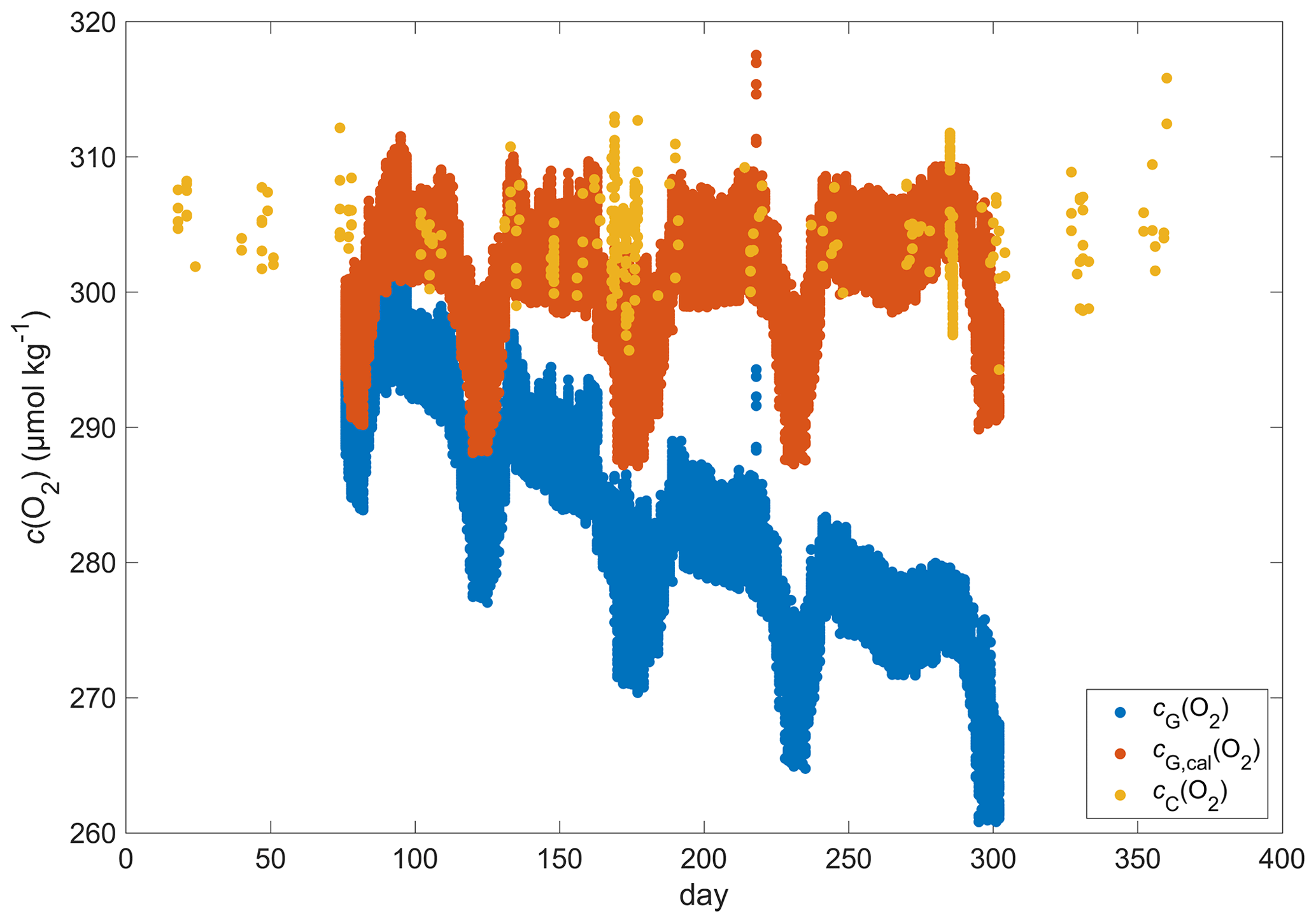
Figure A1Discrete samples cC(O2) (yellow), raw glider oxygen cG(O2) (blue) and drift-corrected glider oxygen cG,cal(O2) (red) for a potential density > 1028 kg m−3 at depths less than 1000 m.
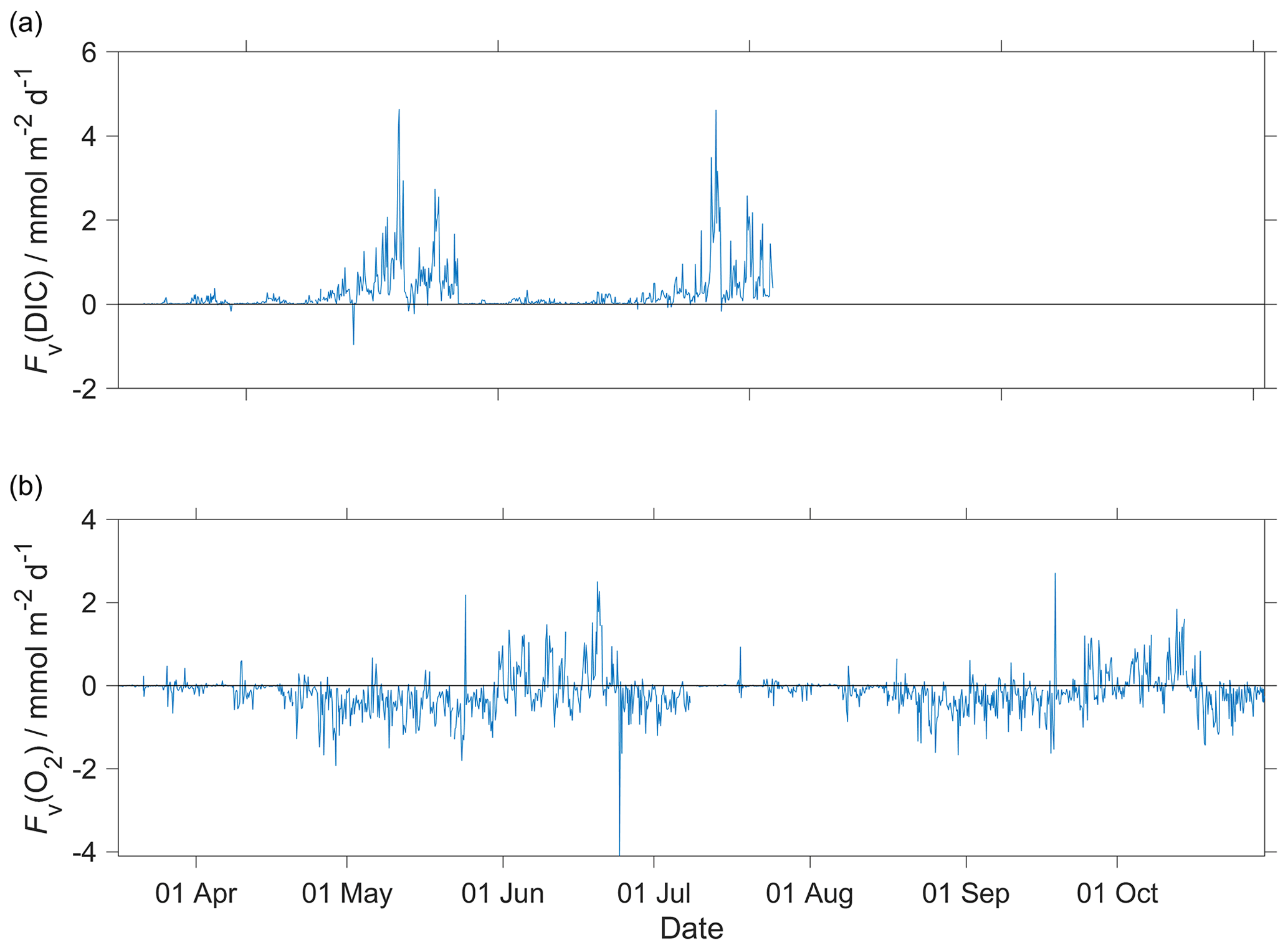
Figure A2Diapycnal mixing (Fv) calculated for the glider descent and ascent for (a) c(DIC) and (b) O2 at the mixed layer depth (zmix) when deeper than 45 m (zlim) and at zlim when zmix was shallower than 45 m. In the calculations, we used a vertical eddy diffusivity (Kz) of 10−5 m2 s−1 (Naveira Garabato et al., 2004).
| Symbols | Quantity (unit) |
| AT | total alkalinity (µmol kg−1) |
| b | backscatter signal (engineering units) |
| c | amount content (µmol kg−1) |
| C | amount concentration (mmol m−3) |
| Chl a | chlorophyll a |
| DIC | dissolved inorganic carbon |
| E | entrainment flux (mmol m−2 d−1) |
| Fv | diapycnal eddy diffusion flux (mmol m−2 d−1) |
| f(CO2) | fugacity of CO2 (µatm) |
| I | inventory (mmol m−2) |
| Kz | diapycnal eddy diffusivity (m2 s−1) |
| N | net community production (mmol m−2 d−1) |
| p(CO2) | partial pressure of CO2 (µatm) |
| S | practical salinity () |
| t | time (s) |
| U | wind speed (m s−1) |
| x | dry mole fraction (mol mol−1) |
| zDCM | depth of the deep chlorophyll maximum (m) |
| zlim | integration depth (m) |
| zmix | mixed layer depth (m) |
| Φ | air–sea flux (mmol m−2 d−1) |
| φ | CO2 optode CalPhase (∘) |
| σ0 | potential density (kg m−3) |
| θ | Celsius temperature (∘C) |
| τ | response time (s) |
The glider data are available from the Norwegian Marine Data Centre (NMDC) at https://doi.org/10.21335/NMDC-1654657723 (Possenti and Castano Primo, 2020).
The CO2 sensor development was led at the University of Gothenburg by DA and AT. Sensor implementation, sampling and analysis for dissolved inorganic carbon content and total alkalinity were led by IS at NORCE. The data were analysed by LP, JK and MPH. LP wrote the first draft manuscript. All authors contributed to further editing and writing.
The authors declare that they have no conflict of interest.
This publication is part of Luca Possenti's PhD project at the University of East Anglia under supervision of Jan Kaiser, Matthew P. Humphreys, Liam Fernand, Socratis Loucaides and Matthew Mowlem. Luca Possenti's PhD project is part of the Next Generation Unmanned Systems Science (NEXUSS) Centre for Doctoral Training which is funded by the Natural Environment Research Council (NERC) and the Engineering and Physical Science Research Council (EPSRC; grant no. NE/N012070/1). We would like to thank the scientists, engineers and crew that contributed to the glider mission and data collection along the glider transect and at Ocean Weather Station M (OWSM). We would also like to thank Kristin Jackson-Misje, who performed all the carbon analyses, as well as Michael Hemming and Bastien Queste for their initial contributions to the data analysis. We are grateful for the comments from the two anonymous reviewers and the editor, which led to a greatly improved paper.
This research has been supported by the Natural Environment Research Council (grant no. NE/N012070/1).
This paper was edited by Mario Hoppema and reviewed by two anonymous referees.
Alkire, M. B., Lee, C., D'Asaro, E., Perry, M. J., Briggs, N., Cetinić, I., and Gray, A.: Net community production and export from Seaglider measurements in the North Atlantic after the spring bloom, J. Geophys. Res.-Oceans, 119, 6121–6139, 2014.
Anderson, L. A.: On the hydrogen and oxygen content of marine phytoplankton, Deep-Sea Res. Pt. I, 42, 1675–1680, 1995.
Anderson, L. A. and Sarmiento, J. L.: Redfield ratios of remineralization determined by nutrient data analysis, Global Biogeochem. Cy., 8, 65–80, 1994.
Atamanchuk, D., Tengberg, A., Thomas, P. J., Hovdenes, J., Apostolidis, A., Huber, C., and Hall, P. O. J.: Performance of a lifetime-based optode for measuring partial pressure of carbon dioxide in natural waters, Limnol. Oceanogr.-Meth., 12, 63–73, https://doi.org/10.4319/lom.2014.12.63, 2014.
Atamanchuk, D., Kononets, M., Thomas, P. J., Hovdenes, J., Tengberg, A., and Hall, P. O. J.: Continuous long-term observations of the carbonate system dynamics in the water column of a temperate fjord, J. Marine Syst., 148, 272–284, https://doi.org/10.1016/j.jmarsys.2015.03.002, 2015a.
Atamanchuk, D., Tengberg, A., Aleynik, D., Fietzek, P., Shitashima, K., Lichtschlag, A., Hall, P. O. J., and Stahl, H.: Detection of CO2 leakage from a simulated sub-seabed storage site using three different types of pCO2 sensors, Int. J. Greenh. Gas Con., 38, 121–134, https://doi.org/10.1016/j.ijggc.2014.10.021, 2015b.
Bakker, D. C. E., Pfeil, B., Landa, C. S., Metzl, N., O'Brien, K. M., Olsen, A., Smith, K., Cosca, C., Harasawa, S., Jones, S. D., Nakaoka, S., Nojiri, Y., Schuster, U., Steinhoff, T., Sweeney, C., Takahashi, T., Tilbrook, B., Wada, C., Wanninkhof, R., Alin, S. R., Balestrini, C. F., Barbero, L., Bates, N. R., Bianchi, A. A., Bonou, F., Boutin, J., Bozec, Y., Burger, E. F., Cai, W.-J., Castle, R. D., Chen, L., Chierici, M., Currie, K., Evans, W., Featherstone, C., Feely, R. A., Fransson, A., Goyet, C., Greenwood, N., Gregor, L., Hankin, S., Hardman-Mountford, N. J., Harlay, J., Hauck, J., Hoppema, M., Humphreys, M. P., Hunt, C. W., Huss, B., Ibánhez, J. S. P., Johannessen, T., Keeling, R., Kitidis, V., Körtzinger, A., Kozyr, A., Krasakopoulou, E., Kuwata, A., Landschützer, P., Lauvset, S. K., Lefèvre, N., Lo Monaco, C., Manke, A., Mathis, J. T., Merlivat, L., Millero, F. J., Monteiro, P. M. S., Munro, D. R., Murata, A., Newberger, T., Omar, A. M., Ono, T., Paterson, K., Pearce, D., Pierrot, D., Robbins, L. L., Saito, S., Salisbury, J., Schlitzer, R., Schneider, B., Schweitzer, R., Sieger, R., Skjelvan, I., Sullivan, K. F., Sutherland, S. C., Sutton, A. J., Tadokoro, K., Telszewski, M., Tuma, M., van Heuven, S. M. A. C., Vandemark, D., Ward, B., Watson, A. J., and Xu, S.: A multi-decade record of high-quality fCO2 data in version 3 of the Surface Ocean CO2 Atlas (SOCAT), Earth Syst. Sci. Data, 8, 383–413, https://doi.org/10.5194/essd-8-383-2016, 2016.
Benson, B. B. and Krause Jr., D.: The concentration and isotopic fractionation of oxygen dissolved in freshwater and seawater in equilibrium with the atmosphere 1, Limnol. Oceanogr., 29, 620–632, https://doi.org/10.4319/lo.1984.29.3.0620, 1984.
Binetti, U., Kaiser, J., Damerell, G. M., Rumyantseva, A., Martin, A. P., Henson, S., and Heywood, K. J.: Net community oxygen production derived from Seaglider deployments at the Porcupine Abyssal Plain site (PAP; northeast Atlantic) in 2012–2013, Prog. Oceanogr., 183, 102293, https://doi.org/10.1016/j.pocean.2020.102293, 2020.
Bittig, H. C. and Körtzinger, A.: Tackling oxygen optode drift: Near-surface and in-air oxygen optode measurements on a float provide an accurate in situ reference, J. Atmos. Ocean. Tech., 32, 1536–1543, https://doi.org/10.1175/JTECH-D-14-00162.1, 2015.
Bittig, H. C., Fiedler, B., Steinhoff, T., and Körtzinger, A.: A novel electrochemical calibration setup for oxygen sensors and its use for the stability assessment of Aanderaa optodes, Limnol. Oceanogr.-Meth., 10, 921–933, https://doi.org/10.4319/lom.2012.10.921, 2012.
Bushinsky, S. M., Takeshita, Y., and Williams, N. L.: Observing Changes in Ocean Carbonate Chemistry: Our Autonomous Future, Current Climate Change Reports, 5, 207–220, https://doi.org/10.1007/s40641-019-00129-8, 2019.
Chu, S. N., Sutton, A. J., Alin, S. R., Lawrence-Slavas, N., Atamanchuk, D., Mickett, J. B., Newton, J. A., Meinig, C., Stalin, S., and Tengberg, A.: Field evaluation of a low-powered, profiling pCO2 system in coastal Washington, Limnol. Oceanogr.-Meth., 18, 280–296, https://doi.org/10.1002/lom3.10354, 2020.
Copin-Montégut, C.: Consumption and production on scales of a few days of inorganic carbon, nitrate and oxygen by the planktonic community: results of continuous measurements at the Dyfamed Station in the northwestern Mediterranean Sea (May 1995), Deep-Sea Res. Pt. I, 47, 447–477, https://doi.org/10.1016/S0967-0637(99)00098-9, 2000.
Degrandpre, M. D.: Measurement of Seawater pCO2 Using a Renewable-Reagent Fiber Optic Sensor with Colorimetric Detection, Anal. Chem., 65, 331–337, https://doi.org/10.1021/ac00052a005, 1993.
Dickson, A. G.: Thermodynamics of the dissociation of boric acid in synthetic seawater from 273.15 to 318.15 K, Deep-Sea Res., 37, 755–766, https://doi.org/10.1016/0198-0149(90)90004-F, 1990.
Dickson, A. G., Afghan, J. D., and Anderson, G. C.: Reference materials for oceanic CO2 analysis: a method for the certification of total alkalinity, Mar. Chem., 80, 185–197, https://doi.org/10.1016/S0304-4203(02)00133-0, 2003.
Dickson, A. G., Sabine, C. L., and Christian, J. R.: Guide to best practices for ocean CO2 measurements, North Pacific Marine Science Organization, Sidney, British Columbia, 2007.
Dlugokencky, E. J., Lang, P. M., Masarie, K. A., Crotwell, A. M., and Crotwell, M. J.: Atmospheric carbon dioxide dry air mole fractions from the NOAA ESRL Carbon Cycle Cooperative Global Air Sampling Network, NOAA ESRL Glob. Monit. Div., Boulder, Colorado, USA, 1968–2014, 2015.
Ducklow, H. W. and Doney, S. C.: What Is the Metabolic State of the Oligotrophic Ocean? A Debate, Annu. Rev. Mar. Sci., 5, 525–533, https://doi.org/10.1146/annurev-marine-121211-172331, 2013.
Falck, E. and Anderson, L. G.: The dynamics of the carbon cycle in the surface water of the Norwegian Sea, Mar. Chem., 94, 43–53, https://doi.org/10.1016/j.marchem.2004.08.009, 2005.
Falck, E. and Gade, G.: Net community production and oxygen fluxes in the Nordic Seas based on O2 budget calculations, Global Biogeochem. Cy., 13, 1117–1126, https://doi.org/10.1029/1999GB900030, 1999.
Fiedler, B., Fietzek, P., Vieira, N., Silva, P., Bittig, H. C., and Körtzinger, A.: In situ CO2 and O2 measurements on a profiling float, J. Atmos. Ocean. Tech., 30, 112–126, https://doi.org/10.1175/JTECH-D-12-00043.1, 2013.
Foltz, G. R., Grodsky, S. A., Carton, J. A., and McPhaden, M. J.: Seasonal mixed layer heat budget of the tropical Atlantic Ocean, J. Geophys. Res.-Oceans, 108, 3146, https://doi.org/10.1029/2002JC001584, 2003.
Friedlingstein, P., Jones, M. W., O'Sullivan, M., Andrew, R. M., Hauck, J., Peters, G. P., Peters, W., Pongratz, J., Sitch, S., Le Quéré, C., Bakker, D. C. E., Canadell, J. G., Ciais, P., Jackson, R. B., Anthoni, P., Barbero, L., Bastos, A., Bastrikov, V., Becker, M., Bopp, L., Buitenhuis, E., Chandra, N., Chevallier, F., Chini, L. P., Currie, K. I., Feely, R. A., Gehlen, M., Gilfillan, D., Gkritzalis, T., Goll, D. S., Gruber, N., Gutekunst, S., Harris, I., Haverd, V., Houghton, R. A., Hurtt, G., Ilyina, T., Jain, A. K., Joetzjer, E., Kaplan, J. O., Kato, E., Klein Goldewijk, K., Korsbakken, J. I., Landschützer, P., Lauvset, S. K., Lefèvre, N., Lenton, A., Lienert, S., Lombardozzi, D., Marland, G., McGuire, P. C., Melton, J. R., Metzl, N., Munro, D. R., Nabel, J. E. M. S., Nakaoka, S.-I., Neill, C., Omar, A. M., Ono, T., Peregon, A., Pierrot, D., Poulter, B., Rehder, G., Resplandy, L., Robertson, E., Rödenbeck, C., Séférian, R., Schwinger, J., Smith, N., Tans, P. P., Tian, H., Tilbrook, B., Tubiello, F. N., van der Werf, G. R., Wiltshire, A. J., and Zaehle, S.: Global Carbon Budget 2019, Earth Syst. Sci. Data, 11, 1783–1838, https://doi.org/10.5194/essd-11-1783-2019, 2019.
Garcia, H. E. and Gordon, L. I.: Oxygen solubility in seawater: Better fitting equations, Limnol. Oceanogr., 37, 1307–1312, https://doi.org/10.4319/lo.1992.37.6.1307, 1992.
Gattuso, J.-P. and Hansson, L.: Ocean acidification, Oxford University Press, Oxford, UK, 2011.
Gislefoss, J. S., Nydal, R., Slagstad, D., Sonninen, E., and Holme, K.: Carbon time series in the Norwegian sea, Deep-Sea Res. Pt. I, 45, 433–460, https://doi.org/10.1016/S0967-0637(97)00093-9, 1998.
Gourcuff, C.: ANFOG Slocum CTD data correction, Australian National Facility for Ocean Gliderrs, Integrated Marine Observing System IMOS, March 2014.
Goyet, C., Walt, D. R., and Brewer, P. G.: Development of a fiber optic sensor for measurement of pCO2 in sea water: design criteria and sea trials, Deep-Sea Res., 39, 1015–1026, https://doi.org/10.1016/0198-0149(92)90037-T, 1992.
Hagebo, M. and Rey, F.: Storage of seawater for nutrients analysis, Fisk. Hav., 4, 1–12, 1984.
Hansen, B. and Østerhus, S.: North Atlantic – Nordic Seas exchanges, Prog. Oceanogr., 45, 109–208, https://doi.org/10.1016/S0079-6611(99)00052-X, 2000.
Hardman-Mountford, N. J., Moore, G., Bakker, D. C. E., Watson, A. J., Schuster, U., Barciela, R., Hines, A., Moncoiffé, G., Brown, J., Dye, S., Blackford, J., Somerfield, P. J., Holt, J., Hydes, D. J., and Aiken, J.: An operational monitoring system to provide indicators of CO2-related variables in the ocean, ICES J. Mar. Sci., 65, 1498–1503, https://doi.org/10.1093/icesjms/fsn110, 2008.
Haskell, W. Z., Hammond, D. E., Prokopenko, M. G., Teel, E. N., Seegers, B. N., Ragan, M. A., Rollins, N., and Jones, B. H.: Net Community Production in a Productive Coastal Ocean From an Autonomous Buoyancy-Driven Glider, J. Geophys. Res.-Oceans, 124, 4188–4207, https://doi.org/10.1029/2019JC015048, 2019.
Hemsley, J. M.: Observations Platforms Buoys, in: North, 2nd Edn., Academic Press, Oxford, UK, 264–267, https://doi.org/10.1016/B978-0-12-382225-3.00256-5, 2003.
Hemsley, V. S., Smyth, T. J., Martin, A. P., Frajka-williams, E., Thompson, A. F., Damerell, G., and Painter, S. C.: Estimating Oceanic Primary Production Using Vertical Irradiance and Chlorophyll Profiles from Ocean Gliders in the North Atlantic, Environ. Sci. Technol., 49, 11612–11621, https://doi.org/10.1021/acs.est.5b00608, 2015.
Jeansson, E., Olsen, A., Eldevik, T., Skjelvan, I., Omar, A. M., Lauvset, S. K., Nilsen, J. E. Ø., Bellerby, R. G. J., Johannessen, T., and Falck, E.: The Nordic Seas carbon budget: Sources, sinks, and uncertainties, Global Biogeochem. Cy., 25, GB4010, https://doi.org/10.1029/2010GB003961, 2011.
Kara, A. B., Rochford, P. A., and Hurlburt, H. E.: An optimal definition for ocean mixed layer depth, J. Geophys. Res.-Oceans, 105, 16803–16821, https://doi.org/10.1029/2000JC900072, 2000.
Kivimäe, C.: Carbon and oxygen fluxes in the Barents and Norwegian Seas: production, air-sea exchange and budget calculations, PhD Dissertation, University of Bergen, Bergen, Norway, 112–130, 2007.
Klimant, I., Huber, C., Liebsch, G., Neurauter, G., Stangelmayer, A., and Wolfbeis, O. S.: Dual lifetime referencing (DLR) – a new scheme for converting fluorescence intensity into a frequency-domain or time-domain information, in: New Trends in Fluorescence Spectroscopy, Springer, Berlin, Heidelberg, 257–274, https://doi.org/10.1007/978-3-642-56853-4_13, 2001.
Körtzinger, A., Thomas, H., Schneider, B., Gronau, N., Mintrop, L., and Duinker, J. C.: At-sea intercomparison of two newly designed underway pCO2 systems – encouraging results, Mar. Chem., 52, 133–145, https://doi.org/10.1016/0304-4203(95)00083-6, 1996.
Körtzinger, A., Koeve, W., Kähler, P., and Mintrop, L.: C:N ratios in the mixed layer during the productive season in the northeast Atlantic Ocean, Deep-Sea Res. Pt. I, 48, 661–688, https://doi.org/10.1016/S0967-0637(00)00051-0, 2001.
Laws, E. A.: Photosynthetic quotients, new production and net community production in the open ocean, Deep-Sea Res., 38, 143–167, https://doi.org/10.1016/0198-0149(91)90059-O, 1991.
Le Quéré, C., Raupach, M. R., Canadell, J. G., Marland, G., Bopp, L., Ciais, P., Conway, T. J., Doney, S. C., Feely, R. A., Foster, P., Friedlingstein, P., Gurney, K., Houghton, R. A., House, J. I., Huntingford, C., Levy, P. E., Lomas, M. R., Majkut, J., Metzl, N., Ometto, J. P., Peters, G. P., Prentice, I. C., Randerson, J. T., Running, S. W., Sarmiento, J. L., Schuster, U., Sitch, S., Takahashi, T., Viovy, N., van der Werf, G. R., and Woodward, F. I.: Trends in the sources and sinks of carbon dioxide, Nat. Geosci., 2, 831–836, https://doi.org/10.1038/ngeo689, 2009.
Lee, K., Tong, L. T., Millero, F. J., Sabine, C. L., Dickson, A. G., Goyet, C., Park, G. H., Wanninkhof, R., Feely, R. A., and Key, R. M.: Global relationships of total alkalinity with salinity and temperature in surface waters of the world's oceans, Geophys. Res. Lett., 33, L19605, https://doi.org/10.1029/2006GL027207, 2006.
Lee, K., Kim, T., Byrne, R. H., Millero, F. J., Feely, R. A., and Liu, Y.: The universal ratio of boron to chlorinity for the North Pacific and North Atlantic oceans, Geochim. Cosmochim. Ac., 74, 1801–1811, https://doi.org/10.1016/j.gca.2009.12.027, 2010.
Lockwood, D., Quay, P. D., Kavanaugh, M. T., Juranek, L. W., and Feely, R. A.: High-resolution estimates of net community production and air-sea CO2 flux in the northeast Pacific, Global Biogeochem. Cy., 26, GB4010, https://doi.org/10.1029/2012GB004380, 2012.
Lueker, T. J., Dickson, A. G., and Keeling, C. D.: Ocean pCO2 calculated from DIC, TA, and the Mehrbach equations for K1 and K2: Validation using laboratory measurements of CO2 in gas and seawater at equilibrium, Abstr. Pap. Am. Chem. S., 217, U848–U848, 2000.
Martz, T. R., Connery, J. G., and Johnson, K. S.: Testing the Honeywell Durafet for seawater pH applications, Limnol. Oceanogr.-Meth., 8, 172–184, https://doi.org/10.4319/lom.2010.8.172, 2010.
Medeot, N., Nair, R., and Gerin, R.: Laboratory Evaluation and Control of Slocum Glider C – T Sensors, J. Atmos. Ocean. Tech., 6, 838–846, https://doi.org/10.1175/2011JTECHO767.1, 2011.
Miloshevich, L.: Development and Validation of a Time-Lag Correction for Vaisala Radiosonde Humidity Measurements, J. Atmos. Ocean. Tech., 21, 1305–1328, https://doi.org/10.1175/1520-0426(2004)021<1305:DAVOAT>2.0.CO;2, 2004.
Monteiro, P. M. S., Schuster, U., Hood, M., Lenton, A., Metzl, N., Olsen, A., Rogers, K., Sabine, C., Takahashi, T., and Tilbrook, B.: A global sea surface carbon observing system: Assessment of changing sea surface CO2 and air-sea CO2 fluxes, Proc. Ocean., 9, 702–714, 2009.
Monterey, G. I. and Levitus, S.: US National Environmental Satellite and Information Service: Seasonal variability of mixed layer depth for the world ocean, US Department of Commerce, National Oceanic and Atmospheric Administration, Silver Spring, MD, 1997.
Naveira Garabato, A. C., Oliver, K. I. C., Watson, A. J., and Messias, M.: Turbulent diapycnal mixing in the Nordic seas, J. Geophys. Res.-Oceans, 109, C12010, https://doi.org/10.1029/2004JC002411, 2004.
Neftel, A., Oeschger, H., Schwander, J., Stauffer, B., and Zumbrunn, R.: Ice core sample measurements give atmospheric CO2 content during the past 40 000 years, Nature, 295, 220–223, https://doi.org/10.1038/295220a0, 1982.
Neuer, S., Cianca, A., Helmke, P., Freudenthal, T., Davenport, R., Meggers, H., and Knoll, M.: Biogeochemistry and hydrography in the eastern subtropical North Atlantic gyre, Results from the European time-series station ESTOC, Prog. Oceanogr., 72, 1–29, https://doi.org/10.1016/j.pocean.2006.08.001, 2007.
Nicholson, D., Emerson, S., and Eriksen, C. C.: Net community production in the deep euphotic zone of the subtropical North Pacific gyre from glider surveys, Limnol. Oceanogr., 53, 2226–2236, https://doi.org/10.4319/lo.2008.53.5_part_2.2226, 2008.
Nicholson, D. P. and Feen, M. L.: Air calibration of an oxygen optode on an underwater glider, Limnol. Oceanogr.-Meth., 15, 495–502, https://doi.org/10.1002/lom3.10177, 2017.
Nilsen, J. E. Ø. and Falck, E.: Variations of mixed layer properties in the Norwegian Sea for the period 1948–1999, Prog. Oceanogr., 70, 58–90, https://doi.org/10.1016/j.pocean.2006.03.014, 2006.
Obata, A., Ishizaka, J., and Endoh, M.: Global verification of critical depth theory for phytoplankton bloom with climatological in situ temperature and satellite ocean color data, J. Geophys. Res.-Oceans, 101, 20657–20667, https://doi.org/10.1029/96JC01734, 1996.
Olsen, A., Key, R. M., van Heuven, S., Lauvset, S. K., Velo, A., Lin, X., Schirnick, C., Kozyr, A., Tanhua, T., Hoppema, M., Jutterström, S., Steinfeldt, R., Jeansson, E., Ishii, M., Pérez, F. F., and Suzuki, T.: The Global Ocean Data Analysis Project version 2 (GLODAPv2) – an internally consistent data product for the world ocean, Earth Syst. Sci. Data, 8, 297–323, https://doi.org/10.5194/essd-8-297-2016, 2016.
Osterroht, C. and Thomas, H.: New production enhanced by nutrient supply from non-Redfield remineralisation of freshly produced organic material, J. Marine Syst., 25, 33–46, https://doi.org/10.1016/S0924-7963(00)00007-5, 2000.
Pachauri, R. K. and Reisinger, A.: IPCC Fourth Assessment Report, 976, available at: https://www.ipcc.ch/site/assets/uploads/2018/03/ar4_wg2_full_report.pdf (last access: 5 February 2019), 2007.
Peeters, F., Atamanchuk, D., Tengberg, A., Encinas-Fernández, J., and Hofmann, H.: Lake metabolism: Comparison of lake metabolic rates estimated from a diel CO2-and the common diel O2-technique, PLoS One, 11, 12, https://doi.org/10.1371/journal.pone.0168393, 2016.
Plant, J. N., Johnson, K. S., Sakamoto, C. M., Jannasch, H. W., Coletti, L. J., Riser, S. C., and Swift, D. D.: Net community production at Ocean Station Papa observed with nitrate and oxygen sensors on profiling floats, Global Biogeochem. Cy., 30, 859–879, https://doi.org/10.1002/2015GB005349, 2016.
Possenti, L. and Castano Primo, R.: Svinøy transect oxygen and dissolved inorganic, NMDC, carbon, University of Bergen, Bergen, Norway, https://doi.org/10.21335/NMDC-1654657723, 2020.
Quay, P., Stutsman, J., and Steinhoff, T.: Primary production and carbon export rates across the subpolar N, Atlantic Ocean basin based on triple oxygen isotope and dissolved O2 and Ar gas measurements, Global Biogeochem. Cy., 26, GB2003, https://doi.org/10.1029/2010GB004003, 2012.
Redfield, A. C.: The influence of organisms on the composition of seawater, The Sea, 2, 26–77, 1963.
Rérolle, V. M. C., Floquet, C. F. A., Harris, A. J. K., Mowlem, M. C., Bellerby, R. R. G. J., and Achterberg, E. P.: Development of a colorimetric microfluidic pH sensor for autonomous seawater measurements, Anal. Chim. Acta, 786, 124–131, https://doi.org/10.1016/j.aca.2013.05.008, 2013.
Reuer, M. K., Barnett, B. A., Bender, M. L., Falkowski, P. G., and Hendricks, M. B.: New estimates of Southern Ocean biological production rates from ratios and the triple isotope composition of O2, Deep-Sea Res. Pt. I, 54, 951–974, https://doi.org/10.1016/j.dsr.2007.02.007, 2007.
Rey, B. F.: Phytoplankton: the grass of the sea, in: The Norwegian Sea Ecosystem, edited by: Skjodal, H. R., Tapir, Trondheim, Norway, 93–112, 2004.
Sabine, C. L., Feely, R. A., Gruber, N., Key, R. M., Lee, K., Bullister, J. L., Wanninkhof, R., Wong, C. S., Wallace, D. W. R., Tilbrook, B., Millero, F. J., Peng, T.-H., Kozyr, A., Ono, T., and Rios, A. F.: The oceanic sink for anthropogenic CO2, Science, 305, 367–371, https://doi.org/10.1126/science.1097403, 2004.
Saderne, V., Fietzek, P., and Herman, P. M. J.: Extreme Variations of pCO2 and pH in a Macrophyte Meadow of the Baltic Sea in Summer: Evidence of the Effect of Photosynthesis and Local Upwelling, PLoS One, 8, 2–9, https://doi.org/10.1371/journal.pone.0062689, 2013.
Saetre, R. and Ljoen, R.: The norwegian coastal current, Port and Ocean Engineering under Arctic Conditions, Technical University of Norway, Bergen, Norway, 1–22, 1972.
Seguro, I., Marca, A. D., Painting, S. J., Shutler, J. D., Suggett, D. J., and Kaiser, J.: High-resolution net and gross biological production during a Celtic Sea spring bloom, Prog. Oceanogr., 177, 101885, https://doi.org/10.1016/j.pocean.2017.12.003, 2019.
Seidel, M. P., Degrandpre, M. D., and Dickson, A. G.: A sensor for in situ indicator-based measurements of seawater pH, Mar. Chem., 109, 18–28, https://doi.org/10.1016/j.marchem.2007.11.013, 2008.
Sharples, J., Ross, O. N., Scott, B. E., Greenstreet, S. P. R., and Fraser, H.: Inter-annual variability in the timing of stratification and the spring bloom in the North-western North Sea, Cont. Shelf Res., 26, 733–751, https://doi.org/10.1016/j.csr.2006.01.011, 2006.
Skjelvan, I., Falck, E., Anderson, L. G., and Rey, F.: Oxygen fluxes in the Norwegian Atlantic Current, Mar. Chem., 73, 291–303, https://doi.org/10.1016/S0304-4203(00)00112-2, 2001.
Skjelvan, I., Anderson, L. G., Falck, E., and Anders, K.: A Review of the Inorganic Carbon Cycle of the Nordic Seas and Barents Sea, The Nordic Seas: An Integrated Perspective, 14, 157, https://doi.org/10.1029/GM158, 2005.
Skjelvan, I., Falck, E., Rey, F., and Kringstad, S. B.: Inorganic carbon time series at Ocean Weather Station M in the Norwegian Sea, Biogeosciences, 5, 549–560, https://doi.org/10.5194/bg-5-549-2008, 2008.
Sprintall, J. and Roemmich, D.: Characterizing the structure of the surface layer in the Pacific Ocean, J. Geophys. Res.-Oceans, 104, 23297–23311, https://doi.org/10.1029/1999JC900179, 1999.
Sutton, A. J., Sabine, C. L., Maenner-Jones, S., Lawrence-Slavas, N., Meinig, C., Feely, R. A., Mathis, J. T., Musielewicz, S., Bott, R., McLain, P. D., Fought, H. J., and Kozyr, A.: A high-frequency atmospheric and seawater pCO2 data set from 14 open-ocean sites using a moored autonomous system, Earth Syst. Sci. Data, 6, 353–366, https://doi.org/10.5194/essd-6-353-2014, 2014.
Swift, J. H.: The arctic waters, in: The Nordic Seas, Springer, New York, NY, ISBN: 978-1-4615-8037-9, 129–154, 1986.
Takahashi, T., Sutherland, S. C., Sweeney, C., Poisson, A., Metzl, N., Tilbrook, B., Bates, N., Wanninkhof, R., Feely, R. A., Sabine, C., Olafsson, J., and Nojiri, Y.: Global sea – air CO2 flux based on climatological surface ocean pCO2, and seasonal biological and temperature effects, Deep-Sea Res. Pt. II, 49, 1601–1622, https://doi.org/10.1016/S0967-0645(02)00003-6, 2002.
Takahashi, T., Sutherland, S. C., Wanninkhof, R., Sweeney, C., Feely, R. A., Chipman, D. W., Hales, B., Friederich, G., Chavez, F., Sabine, C., Watson, A., Bakker, D. C. E., Schuster, U., Yoshikawa-Inoue, H., Ishii, M., Midorikawa, T., Nojiri, Y., Körtzinger, A., Steinhoff, T., Hoppema, M., Olafsson, J., Arnarson, T. S., Johannessen, T., Olsen, A., Bellerby, R., Wong, C. S., Delille, B., Bates, N. R., and de Baar, H. J. W.: Climatological mean and decadal change in surface ocean pCO2, and net sea-air CO2 flux over the global oceans, Deep-Sea Res. Pt. II, 56, 554–577, https://doi.org/10.1016/j.dsr2.2008.12.009, 2009.
Tengberg, A., Hovdenes, J., Andersson, H. J., Brocandel, O., Diaz, R., and Hebert, D.: Evaluation of a lifetime-based optode to measure oxygen in aquatic systems, Limnol. Oceanogr.-Meth., 4, 7–17, https://doi.org/10.4319/lom.2006.4.7, 2006.
Thomas, H., Ittekkot, V., Osterroht, C., and Schneider, B.: Preferential recycling of nutrients – the ocean's way to increase new production and to pass nutrient limitation?, Limnol. Oceanogr., 44, 1999–2004, https://doi.org/10.4319/lo.1999.44.8.1999, 1999.
Thomas, P. J., Atamanchuk, D., Hovdenes, J., and Tengberg, A.: The use of novel optode sensor technologies for monitoring dissolved carbon dioxide and ammonia concentrations under live haul conditions, Aquacult. Eng., 77, 89–96, https://doi.org/10.1016/j.aquaeng.2017.02.004, 2017.
Thompson, R. O. R. Y.: Climatological numerical models of the surface mixed layer of the ocean, J. Phys. Oceanogr., 6, 496–503, 1976.
van Heuven, S., Pierrot, D., Rae, J. W. B., Lewis, E., and Wallace, D. W. R.: MATLAB program developed for CO2 system calculations, Carbon Dioxide Inf. Anal. Center, Oak Ridge Natl. Lab. US Dep. Energy, Oak Ridge, Tennessee, USA, ORNL/CDIAC-105b, 2011.
von Bültzingslöwen, C., McEvoy, A. K., McDonagh, C., MacCraith, B. D., Klimant, I., Krause, C., and Wolfbeis, O. S.: Sol-gel based optical carbon dioxide sensor employing dual luminophore referencing for application in food packaging technology, Analyst, 127, 1478–1483, https://doi.org/10.1039/B207438A, 2002.
Wanninkhof, R.: Relationship between wind speed and gas exchange over the ocean revisited, Limnol. Oceanogr.-Meth., 12, 351–362, https://doi.org/10.4319/lom.2014.12.351, 2014.
Weiss, R. F.: Carbon dioxide in water and seawater: the solubility of a non-ideal gas, Mar. Chem., 2, 203–215, https://doi.org/10.1016/0304-4203(74)90015-2, 1974.
Weiss, R. F. and Price, B. A.: Nitrous oxide solubility in water and seawater, Mar. Chem., 8, 347–359, https://doi.org/10.1016/0304-4203(80)90024-9, 1980.
Woolf, D. K. and Thorpe, S. A.: Bubbles and the air-sea exchange of gases in near-saturation conditions, J. Mar. Res., 49, 435–466, https://doi.org/10.1357/002224091784995765, 1991.