A mosaic of phytoplankton responses across Patagonia, the southeast Pacific and the southwest Atlantic to ash deposition and trace metal release from the Calbuco volcanic eruption in 2015

Following the eruption of the Calbuco volcano in April 2015, an extensive ash plume spread across northern Patagonia and into the southeast Pacific and southwest Atlantic oceans. Here, we report on field surveys conducted in the coastal region receiving the highest ash load following the eruption (Reloncaví Fjord). The fortuitous location of a long-term monitoring station in Reloncaví Fjord provided data to evaluate inshore phytoplankton bloom dynamics and carbonate chemistry during April–May 2015. Satellite-derived chlorophyll a measurements over the ocean regions affected by the ash plume in May 2015 were obtained to determine the spatial–temporal gradients in the offshore phytoplankton response to ash. Additionally, leaching experiments were performed to quantify the release from ash into solution of total alkalinity, trace elements (dissolved Fe, Mn, Pb, Co, Cu, Ni and Cd) and major ions (F⁻, Cl⁻, SO${}_{\mathrm{4}}^{\mathrm{2}-}$, NO${}_{\mathrm{3}}^{-}$, Li⁺, Na⁺, NH${}_{\mathrm{4}}^{+}$, K⁺, Mg²⁺ and Ca²⁺). Within Reloncaví Fjord, integrated peak diatom abundances during the May 2015 austral bloom were approximately 2–4 times higher than usual (up to 1.4 × 10¹¹ cells m⁻², integrated to 15 m depth), with the bloom intensity perhaps moderated due to high ash loadings in the 2 weeks following the eruption. Any mechanistic link between ash deposition and the Reloncaví diatom bloom can, however, only be speculated on due to the lack of data immediately preceding and following the eruption. In the offshore southeast Pacific, a short-duration phytoplankton bloom corresponded closely in space and time to the maximum observed ash plume, potentially in response to Fe fertilisation of a region where phytoplankton growth is typically Fe limited at this time of year. Conversely, no clear fertilisation on the same timescale was found in the area subject to an ash plume over the southwest Atlantic where the availability of fixed nitrogen is thought to limit phytoplankton growth. This was consistent with no significant release of fixed nitrogen (NO_x or NH₄) from Calbuco ash.

In addition to the release of nanomolar concentrations of dissolved Fe from ash suspended in seawater, it was observed that low loadings (< 5 mg L⁻¹) of ash were an unusually prolific source of Fe(II) into chilled seawater (up to 1.0 µmol Fe g⁻¹), producing a pulse of Fe(II) typically released mainly during the first minute after addition to seawater. This release would not be detected (as Fe(II) or dissolved Fe) following standard leaching protocols at room temperature. A pulse of Fe(II) release upon addition of Calbuco ash to seawater made it an unusually efficient dissolved Fe source. The fraction of dissolved Fe released as Fe(II) from Calbuco ash (∼ 18 %–38 %) was roughly comparable to literature values for Fe released into seawater from aerosols collected over the Pacific Ocean following long-range atmospheric transport.

1 Introduction

Volcanic ash has long been considered a large, intermittent source of trace metals to the ocean (Frogner et al., 2001; Sarmiento, 1993; Watson, 1997), and its deposition is now deemed a sporadic generally low-macronutrient, high-micronutrient supply mechanism (Ayris and Delmelle, 2012; Jones and Gislason, 2008; Lin et al., 2011). As volcanic ash can be a regionally significant source of allochthonous inorganic material to affected water bodies, volcanic eruptions have the potential to dramatically change light availability, the carbonate system, properties of sinking particles and ecosystem dynamics (Hoffmann et al., 2012; Newcomb and Flagg, 1983; Stewart et al., 2006). Surveys directly underneath the ash plume from the 2010 eruption of Eyjafjallajökull (Iceland) over the North Atlantic found, among other biogeochemical perturbations, high dissolved Fe (dFe) concentrations of up to 10 nM in affected surface seawater (Achterberg et al., 2013) which could potentially result in enhanced primary production. The greatest potential positive effect of ash deposition on marine productivity would generally be expected in high-nitrate, low-chlorophyll (HNLC) areas of the ocean (Hamme et al., 2010; Mélançon et al., 2014), where low Fe concentrations are a major factor limiting primary production (Martin et al., 1990; Moore et al., 2013). Therefore, special interest is placed on the ability of volcanic ash to release dFe, and other bio-essential trace metals such as Mn (Achterberg et al., 2013; Browning et al., 2014; Hoffmann et al., 2012), into seawater. In contrast, apart from inducing light limitation, there are several adverse effects of ash deposition on aquatic organisms; these include metal toxicity (Ermolin et al., 2018), particularly under high dust loading (Hoffmann et al., 2012), and the ingestion of ash particles by filter-feeders, phagotrophic organisms or fish (Newcomb and Flagg, 1983; Wolinski et al., 2013). Transient shifts to low pH have also been reported in some (but not all) ash leaching experiments and in some freshwater bodies following intense ash deposition events, suggesting that significant ash deposition on weakly buffered aquatic environments can also impact and perturb their carbonate system (Duggen et al., 2010; Jones and Gislason, 2008; Newcomb and Flagg, 1983). Therefore, the greatest negative impact of ash on primary producers would be expected closest to the source, where the ash loading is highest, and in areas where macronutrients or light, rather than trace elements, limit primary production.

In contrast to the 2010 Eyjafjallajökull plume over the North Atlantic, the 2015 ash plume from the Calbuco eruption (northern Patagonia, Chile) was predominantly deposited over an inshore and coastal region (Romero et al., 2016) (Fig. 1). This led to visible high ash loadings in affected surface waters in the weeks after the eruption (Fig. 2), providing a case study for a concentrated ash deposition event in a coastal system: Reloncaví Fjord, which is the northernmost fjord of Patagonia. It receives the direct discharge from three major rivers, creating a highly stratified and productive fjord system in terms of both phytoplankton biomass and aquaculture production of mussels (González et al., 2010; Molinet et al., 2017; Yevenes et al., 2019). Here, we combine in situ observations from moored arrays, which were fortuitously deployed in Reloncaví Fjord (Vergara-Jara et al., 2019), with satellite-derived chlorophyll data for offshore regions subject to ash deposition and leaching experiments carried out on ash collected from the fjord region in order to investigate the inorganic consequences of ash addition to natural waters. We thereby evaluate the potential positive and negative effects of ash from the 2015 Calbuco eruption on marine phytoplankton in three geographical regions: Reloncaví Fjord and the areas of the southeast Pacific and southwest Atlantic oceans beneath the most intense ash plume.

2 Materials and methods

2.1 Study area

The Calbuco volcano (Fig. 1) is located in a region with large freshwater reservoirs and in close proximity to Reloncaví Fjord. The predominant bedrock type is andesite (López-Escobar et al., 1995). Reloncaví Fjord is 55 km long and receives freshwater from three main rivers, the Puelo, Petrohué, and Cochamó, with mean stream flows of 650, 350 and 100 m³ s⁻¹ respectively (León-Muñoz et al., 2013). River discharge strongly influences seasonal patterns of primary production across the region, supplying silicic acid and strongly stratifying the water column (Castillo et al., 2016; González et al., 2010; Torres et al., 2014). Seasonal changes in light availability rather than macronutrient supply are thought to control marine primary production across the Reloncaví region, with high marine primary production (> 1 g C m⁻² d⁻¹) throughout austral spring, summer and early autumn (González et al., 2010).

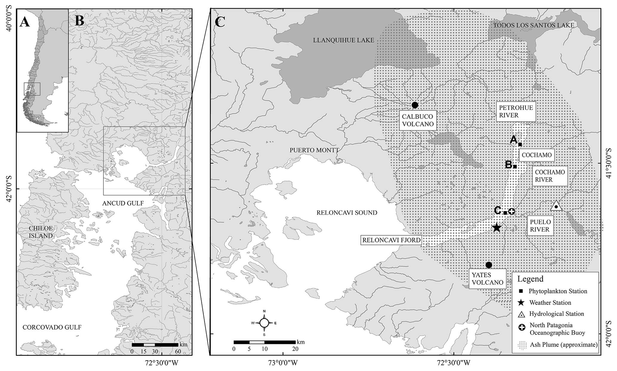
Figure 1 The Calbuco region showing the location of Reloncaví Fjord, three major rivers (the Petrohué, Cochamó and Puelo) discharging into the fjord, the three stations (black squares; panel c) used to assess changes in phytoplankton abundance following the eruption, a hydrological station that monitors the Puelo River flow, a weather station and the location of a long-term mooring within the fjord. The approximate extent of the ash plume in the week following the first eruption is illustrated, as estimated in technical reports issued by the Servicio Nacional de Geología y Minería (Chile).

On 22 April 2015 the Calbuco volcano erupted after 54 years of dormancy. Two major eruption pulses lasted < 2 h on 22 April and 6 h on 23 April, releasing a total volume of 0.27 km³ of ash which was projected up to 20 km a.s.l. (above sea level) (Van Eaton et al., 2016; Romero et al., 2016). Ash layers that were several centimetres thick were deposited mainly to the northeast of the volcano in subsequent days (Romero et al., 2016). A smaller eruption occurred on 30 April projecting ash 4–5 km a.s.l. which was then mainly deposited south of the volcano. Smaller volumes of ash were released semi-continuously for 3 weeks after the main eruption, leading to intermittent ash deposition events. Fortuitously, as part of a long-term deployment, an ocean acidification buoy in the middle of Reloncaví Fjord (Vergara-Jara et al., 2019) and an associated meteorological station close to the volcano (Fig. 1) were well placed to assess the impact of ash deposition immediately after the eruption. To complement data from these facilities, after the regional evacuation order was removed, weekly sampling campaigns were conducted in the fjord commencing 1 week after the eruption. The National Geology and Mining Service (Servicio Nacional de Geología y Minería, SERNAGEOMIN) produced daily technical reports including the estimated area of ash dispersion (http://sitiohistorico.sernageomin.cl/volcan.php?pagina=4&iId=3, last access: 1 February 2021). This information was used to create a reference aerial extent of ash deposition for the week after the eruption (Fig. 1c). This approximation represents a full week of coverage for this dynamic feature.

2.2 Ash samples – trace metal leaching experiments

On 6 May (2015, Cochamó, Chile, approximately 30 km from the volcano) after the third (and smallest) eruptive pulse of ash from the Calbuco volcano (Fig. 2a) and with the volcano still emitting material, ash was collected using a plastic tray wrapped with plastic sheeting (40 cm × 94 cm). The plasticware was left outside for 24 h until sufficient ash (∼ 500 g) was collected to provide a bulk sample. Ambient weather over the period of ash collection (and the preceding day) was dry (no precipitation). The collected ash was double sealed in low-density polyethylene (LDPE) plastic bags and stored in the dark. A subsample was analysed for particle size using a Mastersizer 2000 at the University of Chile.

Ash may affect in situ phytoplankton dynamics in several ways – for example, by moderating the carbonate system, macronutrient availability and/or micronutrient availability. As micronutrient (e.g. Fe and Mn) availability is expected to be the main chemical mechanism via which phytoplankton dynamics in the offshore marine environment could be affected, we primarily focus our investigation on the release of dissolved trace metals from ash in seawater. However, to rule out other potential effects, we also conduct complementary leaches to assess the significance of changes to total alkalinity and macronutrient availability (Table 1). For trace metal leaches, a variety of methods have been used in the literature (Duggen et al., 2010; Witham et al., 2005) depending on the purpose of specific studies. Deionised water leaches with ash loadings that are high in an offshore environmental context are preferable for intercomparison studies. The trace metals released under such conditions are, however, difficult to compare quantitatively to metal exchange processes in the ambient marine environment, especially for elements such as Fe where solubility is strongly influenced by pH, salinity and the nature of dissolved organic carbon present (Baker and Croot, 2010). For prior work conducted specifically using volcanic ash in seawater, three main methods have been employed: suspension experiments followed by analysis of the leachate, flow-through reactors and continuous voltammetric determination of dFe concentrations in situ during suspension experiments (Table S1 in the Supplement). The most commonly used ash : solute ratio in prior seawater experiments is 1:400 (g : mL), with leach lengths varying from 15 min to 24 h (Table S1). Conversely, incubation experiments designed to test the response of marine phytoplankton to ash deposition have used lower ash : solute ratios of 1:400 to 1:10⁷ which are based on estimates of the ash loading expected to be mixed within the offshore surface mixed layer underneath ash plumes (Browning et al., 2014; Hoffmann et al., 2012). Existing data suggest that the ash : solute ratio is not a major factor in determining the release behaviour of Fe from ash; nevertheless, this is acknowledged to be difficult to assess due to other differences between experimental set-ups used to date (Duggen et al., 2010). Both the age of particles since collection and the organic carbon content of seawater are, however, known to be critical factors influencing the exchange of Fe (and other trace elements) following any aerosol deposition into seawater (Baker and Croot, 2010; Duggen et al., 2010). Whilst the UV treatment of seawater has been used in some experiments (to remove a large part of any natural organic ligands present, Duggen et al., 2007; Jones and Gislason, 2008), and a strong synthetic organic ligand has been added in others (to impede dissolved Fe precipitation; Duggen et al., 2007; Olgun et al., 2011; Simonella et al., 2015), to improve reproducibility and standardisation, these steps are not well suited specifically for investigating the release of Fe(II) from ash. Thus, in this study, we adopt ash : solute ratios comparable to the lower end of the range used in leaching experiments and comparable to the range used in incubation experiments. Seawater was used after prolonged storage in the dark (to reduce biological activity to low background levels) and without UV treatment (to maintain an environmentally relevant level of natural organic material in solution). A short leaching time (10 min + filtration) was adopted to minimise bottle effects and recognising that most prior work suggests a large fraction of Fe release occurs on short timescales (minutes), followed by more gradual changes on timescales of hours to days (Duggen et al., 2007; Frogner et al., 2001; Jones and Gislason, 2008).

A variety of leaches were conducted in deionised water, brackish (fjord) water or offshore South Atlantic seawater (Table 1) with the choice of leaching conditions based on the expected environmental significance in different water masses. Offshore oligotrophic seawater for incubation experiments was collected from an underway transect of the mid-South Atlantic (across 40^∘ S) using a towfish and trace metal clean tubing in a 1 m³ high-density polyethylene tank which had been pre-rinsed with 1 M HCl. This water was stored in the dark for > 12 months prior to use in leaching experiments and was filtered (AcroPak1000 capsule $\mathrm{0.8}/\mathrm{0.2}$ µm filters) when subsampling a batch for use in all leaching experiments. All labware for trace metal leaching experiments was pre-cleaned with Mucasol and 1 M HCl. The 125 mL LDPE bottles (Nalgene) for trace metal leach experiments were pre-cleaned using a three-stage procedure with three deionised water (Milli-Q, Millipore, conductivity 18.2 MΩ cm⁻¹) rinses after each stage (3 d in Mucasol, 1 week in 1 M HCl, 1 week in 1 M HNO₃).

Leach experiments were conducted by adding a pre-weighed mass of ash into 100 mL South Atlantic seawater, gently mixing the suspension for 10 min, and then syringe filtering the suspension (0.2 µm, polyvinylidene fluoride, Millipore). Eight different ash loadings from 2 to 50 mg L⁻¹ were used, which were selected to be environmentally relevant and comparable to prior incubation experiments, with each treatment run in triplicate. Samples for dissolved trace metals (Fe, Cd, Pb, Ni, Cu, Co and Mn) were acidified within 1 d of collection by the addition of 140 µL concentrated HCl (UpA grade, ROMIL) and analysed by inductively coupled plasma mass spectroscopy following pre-concentration exactly as per Rapp et al. (2017).

Leach experiments specifically to measure Fe(II) release were conducted in a similar manner but in cold seawater with continuous in-line analysis (5–7 ^∘C; see Table S2 in the Supplement) due to the rapid oxidation rate of Fe(II) at room temperature (∼ 21 ^∘C), which makes the accurate measurement of Fe(II) concentrations challenging (Millero et al., 1987). For these experiments, a pre-weighed mass of ash was added to 250 mL of South Atlantic seawater and manually shaken for approximately 1 min, using an expanded loading range from 0.2 to 4000 mg L⁻¹. Fe(II) was measured via flow injection analysis using luminol chemiluminescence (Jones et al., 2013) without pre-concentration or filtration. The inflow line feeding the flow injection apparatus was positioned inside the ash suspension immediately after mixing and measurements begun thereafter at a 2 min resolution. Reported mean values (± standard deviation) are determined from the Fe(II) concentrations measured 2–30 min after adding ash into solution. Calibrations were run daily using standard additions of 0.2–10 nM Fe(II) to aged South Atlantic seawater at the same temperature with integrated peak area used to construct calibration curves. Following each leaching experiment, the apparatus was rinsed with 0.1 M HCl (reagent grade) followed by flushing with deionised water to ensure the removal of ash particles. Blank measurements before and after Fe(II) measurements from experiments with different ash loadings verified that there was no discernable interference from ash particles in the Fe(II) flow-through measurements. Fe(II) leaches were conducted 2 weeks, 4 months and 9 months after the eruption. Fe(II) leaches 2 weeks after the eruption were run for 30 min. Fe(II) leaches 4 or 9 months after the eruption were run for 1 h to further investigate the temporal development of the Fe(II) concentration. The trace metal leach experiments (above) were conducted at the same time as the first Fe(II) incubation experiments (2 weeks after ash collection).

For trace metal leaches, the initial (mean ± standard deviation) dissolved trace metal concentrations were deducted from the final concentrations, in order to calculate the net change as a result of ash addition. For Fe(II) measurements, background levels of Fe(II) were below detection (< 0.1 nM) and so no deduction was made.

2.3 Ash samples – deionised and brackish water leaching experiments

Fresh brackish subsurface water from the Patagonia study region was obtained from the Aysén Fjord, at Ensenada Baja (45^∘21^′ S, 72^∘40^′ W; salinity 16.3), close to the Coyhaique laboratory (Aysén region, Chile) and free from the influence of ash from the 2015 eruption. The oceanographic conditions in these waters are similar to the adjacent Reloncaví Fjord (Cáceres et al., 2002). Deionised water, along with the Aysén Fjord brackish water, were used for leaching experiments using two size fractions of ash, following the general recommendations of Duggen et al. (2010) and Witham et al. (2005), to consider the effects of different size fractions and leachates. Leaches were conducted in 50 mL LDPE bottles filled with either 40 mL of brackish or deionised water with four replicates of each treatment. Bottles were incubated inside a mixer at room temperature after the addition of 0.18 g of ash, using two ash size fractions (< 63 and 250–1000 µm) which were separated using sieves (ASTM E11 specification, W. S. Tyler). The mass distribution of the ash as determined by sieving was 4.54 % > 2360 µm, 6.85 % < 2360 and > 1000 µm, 31.12 % < 1000 and > 250 µm, 24.14 % < 250 and > 125 µm, 18.04 % < 125 and > 63 µm, and 15.31 % < 63 µm. Thus, the dominant size fraction by mass was the 250–1000 µm fraction, which was analysed in addition to the finest fraction (< 63 µm) with the greatest surface area to mass ratio. The sampling times were at time zero (defined as just after the addition of the ash and a few minutes of mixing) and 2 and 24 h later. Leaching experiments conducted with brackish water were analysed for total alkalinity (A_T) via a potentiometric titration using reference standards (Haraldsson et al., 1997), ensuring a reproducibility of < 2 µmol kg⁻¹. For the deionised water leaching experiment, A_T was analysed by titration of unfiltered 5 mL subsamples to a pH 4.5 end point (bromocresol green–methyl red) using a Dosimat (Metrohm Inc) and 0.02 N H₂SO₄ titrant. Alkalinity was calculated as CaCO₃ equivalents following APHA (American Public Health Association) 2005 Method 2320 (2320 alkalinity and titration method). Additional 5 mL subsamples were filtered, stored at 4 ^∘C and analysed within 3 d for major ions (F⁻, Cl⁻, SO${}_{\mathrm{4}}^{\mathrm{2}-}$, NO${}_{\mathrm{3}}^{-}$, Li⁺, Na⁺, NH${}_{\mathrm{4}}^{+}$, K⁺, Mg²⁺ and Ca²⁺) using a Dionex™ 5000 ion chromatography system with eluent generation (APHA). All measurements were then corrected for initial water concentrations prior to ash addition. Saturation indices for species in solution following leaching from < 63 µm ash particles were obtained from the MINTEQ 3.1. IAP (ion activity product) chemical equilibrium model (see Table S6 in the Supplement).

Table 1 Summary of different leaching experiments and samples.

2.4 Environmental data – continuous Reloncaví Fjord monitoring

High-temporal-resolution (hourly) in situ measurements were taken in the Reloncaví Fjord (Fig. 1c, North Patagonia Oceanographic Buoy) at 3 m depth using submersible autonomous moored instrument (SAMI) sensors that measured spectrophotometric CO₂ and pH (DeGrandpre et al., 1995; Seidel et al., 2008) (Sunburst Sensors, LLC) and an SBE 37 MicroCAT CTD-ODO (Sea-Bird Electronics) that measured temperature, conductivity, depth and dissolved O₂, as per Vergara-Jara et al. (2019). Sensor maintenance and quality control is described by Vergara-Jara et al. (2019). The error in pCO₂ concentrations is estimated to be 5 % at most and arises mainly due to a non-linear sensor response and reduced sensitivity at high pCO₂ levels > 1500 ppm (DeGrandpre et al., 1999). The SAMI pH instruments used an accuracy test instead of a calibration procedure (Seidel et al., 2008). With the broad pH and salinity range found in the fjord, pH values are subject to a maximum error of ± 0.02 (Mosley et al., 2004).

A meteorological station (HOBO U30, Fig. 1) measured air temperature, solar radiation, wind speed and direction, rainfall, and barometric pressure every 5 min. Puelo River streamflow was obtained from the Carrera Basilio hydrological station (Fig. 1), run by Dirección General de Aguas de Chile, via a data request (submitted via https://snia.mop.gob.cl/BNAConsultas/reportes, last access: 22 February 2019).

2.5 Field surveys in Reloncaví Fjord post-eruption

During May 2015, weekly field campaigns were undertaken in the Reloncaví Fjord. Phytoplankton samples were collected at three depths (1, 5 and 10 m) for taxonomic characterisation and abundance determination at three stations (Fig. 1c) using a 5 L GO-FLO bottle. Samples for cell counts were stored in clear plastic bottles (300 mL) and preserved in a Lugol iodine solution. From each sample, a 10 mL subsample was placed in a sedimentation chamber and left to settle for 16 h. The complete chamber bottom was scanned at 200× to enumerate the organisms, and the result was expressed as number of phytoplankton cells per litre of seawater (Hasle, 1978). Phytoplankton were identified to genus or species level, when possible, and divided into diatoms and dinoflagellates. Samples were analysed using an Olympus CKX41 inverted phase contrast microscope and the Utermöhl method (Utermöhl, 1958). The phytoplankton community composition was then statistically analysed in R (R Core Team, 2020; R Studio V 1.2.5033) using general linear models in order to find statistically significant differences between dates and group abundances. Additionally, as part of a long-term monitoring programme at station C (Fig. 1c), chlorophyll a samples were retained from six depths (1, 3, 5, 7, 10 and 15 m) on six occasions during March–May 2015. Chlorophyll a was determined by fluorometry after filtering 250 mL of sampled water through GF/F filters (Whatman) as per Welschmeyer (1994). Two additional profiles close to station C were obtained from Yevenes et al. (2019). Integrated chlorophyll a (mg m⁻²) and diatom abundance (cells m⁻²) were determined to 15 m depth. Chlorophyll a within Reloncaví Fjord is invariably concentrated in the upper ∼ 10 m (González et al., 2010; Yevenes et al., 2019); thus, for comparison to prior reported data integrated to 10 m, only a small difference is anticipated. For all profiles considered herein, there is a 20 % difference between integrating to 10 m or 15 m depth.

2.6 Satellite data

Daily, 4 km resolution chlorophyll a images from the MODIS Aqua sensor (Ocean Color Index, OCI, algorithm; Hu et al., 2012) were downloaded from the NASA Ocean Color website (https://oceancolor.gsfc.nasa.gov, last access: 1 June 2020) for the period from 4 April to 2 May 2015. As the UV aerosol index largely reflects strongly UV-absorbing (dust) aerosols (Torres et al., 2007), this was used as a proxy for the spatial extent and loading of the ash plume. The UV aerosol index product from the Ozone Monitoring Instrument (OMI) on the Earth Observing System (EOS) Aura was downloaded for the same time period. Daily images were composited into 5 d mean averages.

3 Results

3.1 In situ observations

The Calbuco ash plume reached up to a height of 20 km and was dispersed hundreds of kilometres across Patagonia and the Pacific and Atlantic oceans (Fig. 2) (Van Eaton et al., 2016; Reckziegel et al., 2016; Romero et al., 2016). The ash loading in water bodies near the cone was visually observed to be high, especially near the Petrohué River catchment that drains into the head of the Reloncaví Fjord. This ash loading in the fjord was clearly visible on 6 May 2015 when ash samples were collected for leaching experiments (Fig. 2).

Figure 2 (a) Calbuco volcano ash plume 6 May 2015. (b) Reloncaví Fjord water with atypical high turbidity due to the ash loading, Cochamó town 6 May. (c) Ash cloud visible on MODIS Aqua satellite from the NASA Earth Observatory, 23 April (http://earthobservatory.nasa.gov/NaturalHazards/view.php?id=85767&eocn=home&eoci=nh, last access: 1 February 2021). The highlighted box in panel (c) corresponds to Fig. 1c.

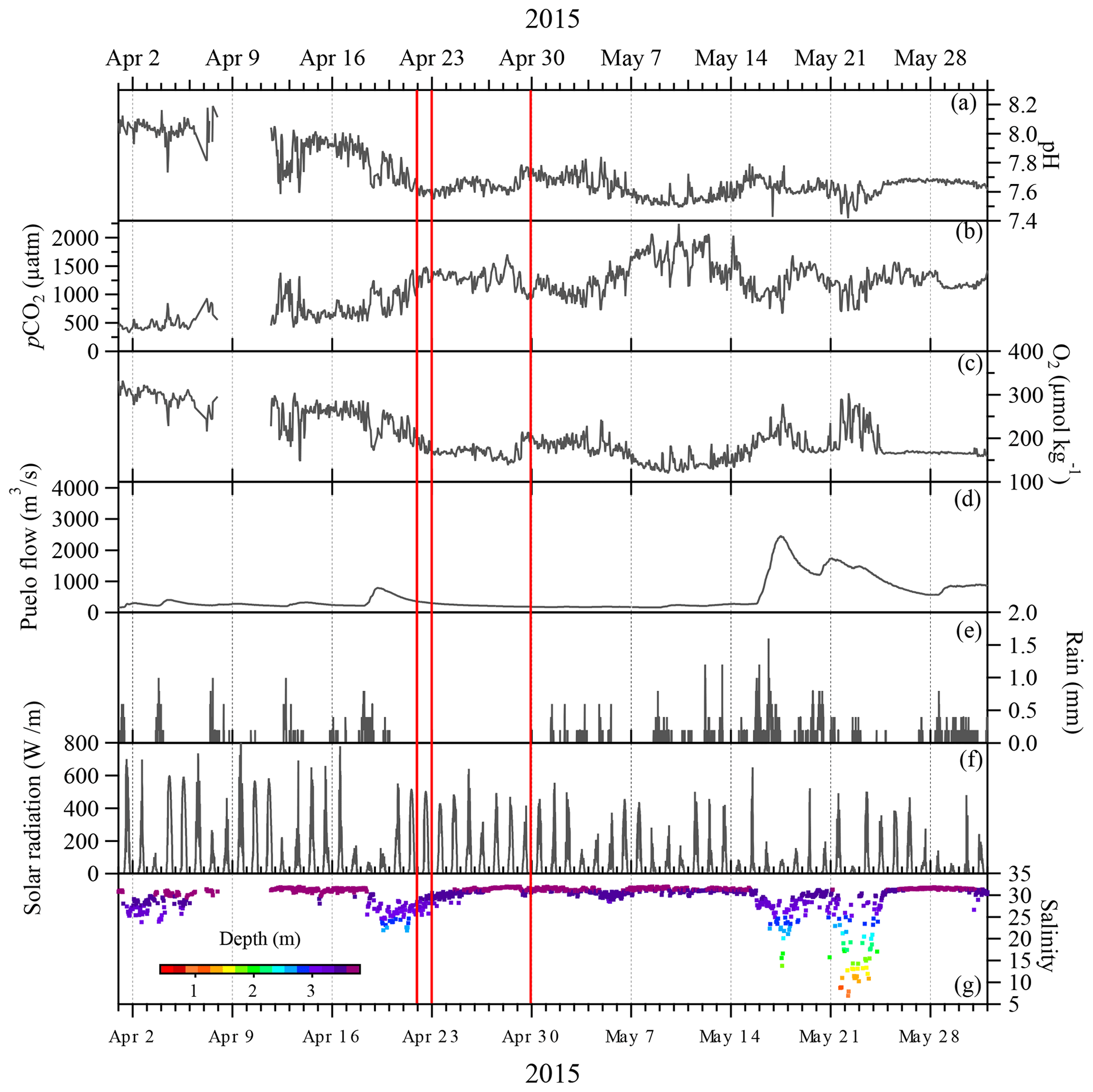
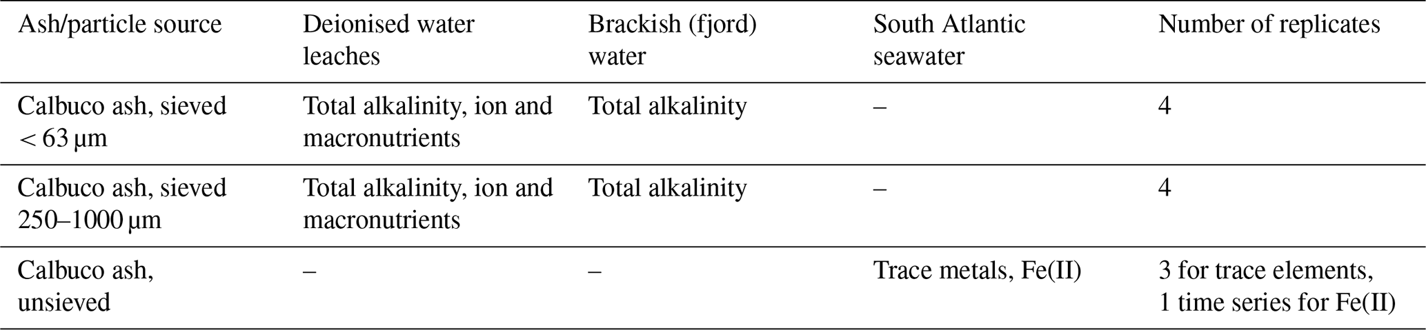
Figure 3 Continuous data from the Reloncaví Fjord mooring and nearby hydrological and weather stations for April–May 2015. The vertical red lines mark the eruption dates. All locations are marked in Fig. 1. Carbonate chemistry and salinity data are from Vergara-Jara et al. (2019). Wind and tidal mixing caused small changes in the depth of the sensors which are shown alongside the salinity data.

Carbonate chemistry data from the Reloncaví Fjord mooring demonstrated that the pH declined and the pCO₂ increased in the week prior to the first eruption (22 April, Fig. 3). Oxygen and pH reached a minimum and pCO₂ reached a maximum during the time period from 7 to 14 May, which indicates a state of high respiration. In this stratified environment, the brackish fjord surface layer generally has low pH and high pCO₂, with seasonal changes in salinity and respiration leading to a large annual range of pCO₂ and pH (Vergara-Jara et al., 2019). The depth of the sensors varied temporally due to changes in tides and river flow. This accounts for some of the variation in measured salinity due to the strong salinity gradient with depth in the brackish surface waters (Fig. 3). Therefore, any changes in pCO₂ or pH occurring as a direct result of the eruptions (or associated ash deposition) are challenging to distinguish from background variation due to short-term (intra-day) or seasonal shifts in the carbonate system which are pronounced in this dynamic and strongly freshwater-influenced environment (Fig. 3). Freshwater discharge from the Puelo increased sharply from 16 May which is an annually recurring event (González et al., 2010).

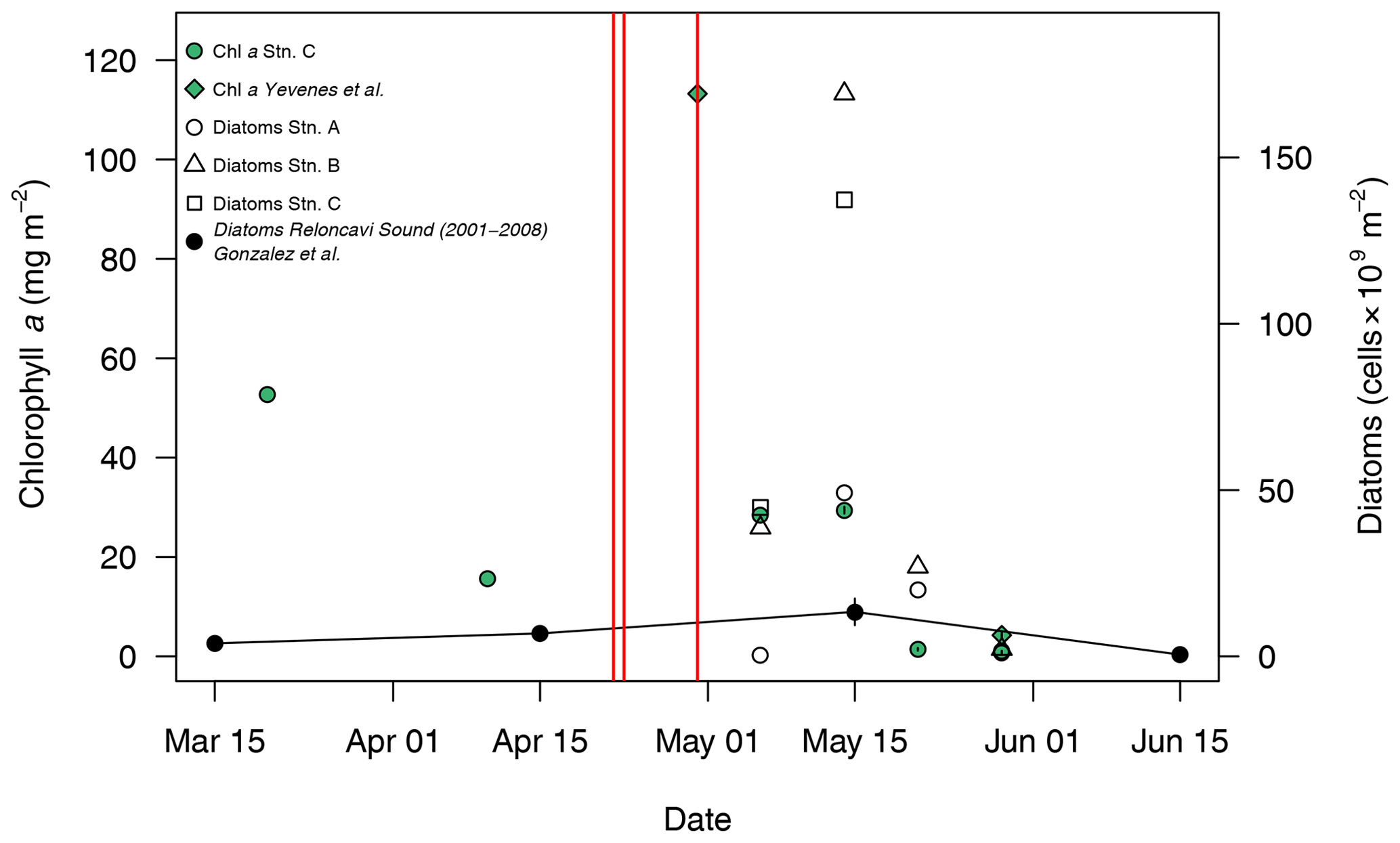
Figure 4 Changes in integrated (0–15 m) diatom abundance and chlorophyll a for Reloncaví Fjord in April–May 2015. Locations are as per Fig. 1; the eruption dates are marked with red lines. Historical diatom data from Reloncaví Sound (2001–2008, integrated to 10 m depth, mean ± standard error, González et al., 2010) and additional chlorophyll data from 2015 (“Station 3” from Yevenes et al., 2019, approximately corresponding to station C herein) are also shown.

3.2 Phytoplankton in Reloncaví Fjord post-eruption

Phytoplankton abundances observed in May 2015 within Reloncaví Fjord were assessed by diatom cell counts and chlorophyll a concentrations (Table S3 in the Supplement) and were proportionate to or higher than those previously observed in the region (Fig. 4). When comparing observations to prior data from González et al. (2010), it should be noted that there is a slight depth discrepancy (earlier work was integrated to 10 m depth rather than the 15 m used herein). However, as the phytoplankton bloom is overwhelmingly present within the upper 10 m, these data do provide a useful comparison. Diatom abundance integrated to 15 m depth peaked at stations B and C around 14 May, with notably lower abundances at the innermost station A (Fig. 4). The highest measured chlorophyll a concentrations were on 30 April at station C; chlorophyll a values then declined to much lower concentrations in late May, which is expected from patterns in regional primary production (González et al., 2010). No measurements were available for 10–30 April 2015 (Fig. 4); thus, it is not possible to determine the timing of the onset of the austral autumn phytoplankton bloom with respect to the volcanic eruptions from the available chlorophyll a or diatom data. However, within this time period, the mooring at station C (Fig. 3) did record a modest increase in pH and O₂ from 28 to 29 April, during a time period when river discharge and salinity were stable, which could be indicative of the autumn phytoplankton bloom onset.

3.3 Total alkalinity and macronutrients in leach experiments

Size analysis of the collected ash determined a mean particle diameter of 339 µm. Small ash particles (< 63 µm) resulted in minor or no significant changes to A_T in brackish fjord waters (Fig. 5). With larger ash particles (250–1000 µm), no effect was evident. Conversely, a leaching experiment with deionised water showed a small increase in A_T (Fig. 5) for both size fractions. By increasing the A_T of freshwater, ash would act to increase the buffering capacity of river outflow into a typically weak carbonate system like the Reloncaví Fjord (Vergara-Jara et al., 2019). However, the absolute change in A_T was relatively small despite the large ash loading used in all incubations (< 20 µmol kg⁻¹ A_T for ash loading > 4 g L⁻¹); therefore, it is expected that the direct effect of ash on A_T in situ was limited. Other effects on carbonate chemistry may, however, arise due to ash moderating the timing and intensity of primary production and, thus, biological pCO₂ drawdown.

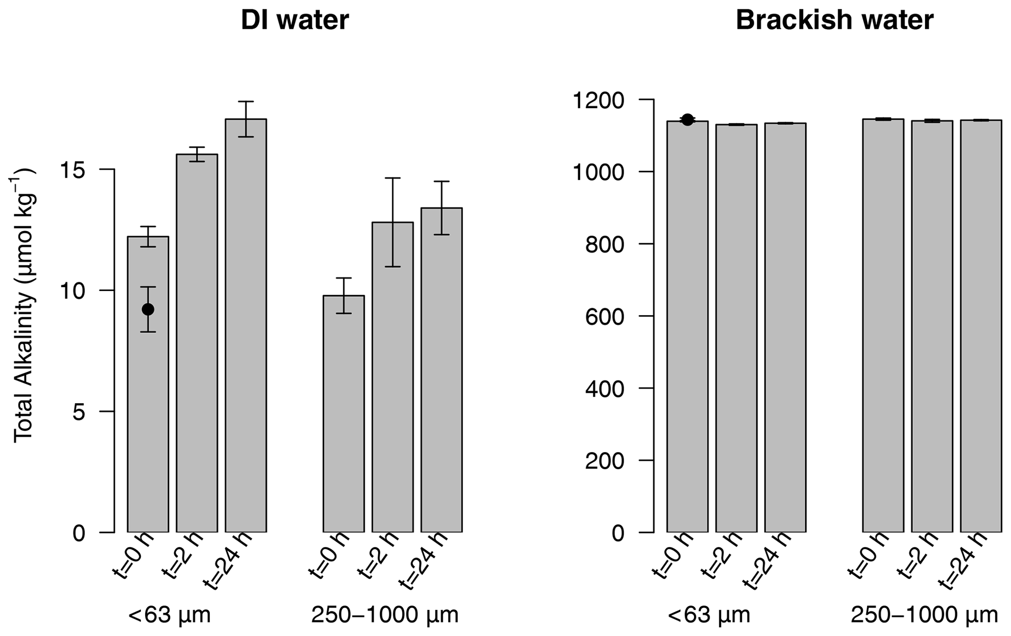
Figure 5 Total alkalinity released after leaching 4.5 g L⁻¹ of ash of two size fractions (< 63 and 250–1000 µm) in deionised water (DI water) and brackish water. T₀ is “time zero” and was measured after 1 min of mixing; T_2H was measured after 2 h of mixing; T_24H was measured after 24 h of mixing. n=4 for all treatments (mean ± standard deviation plotted). The initial (pre-ash addition) alkalinity is marked by a black dot superimposed on the left T₀. Source data are provided in the Supplement (Table S4).

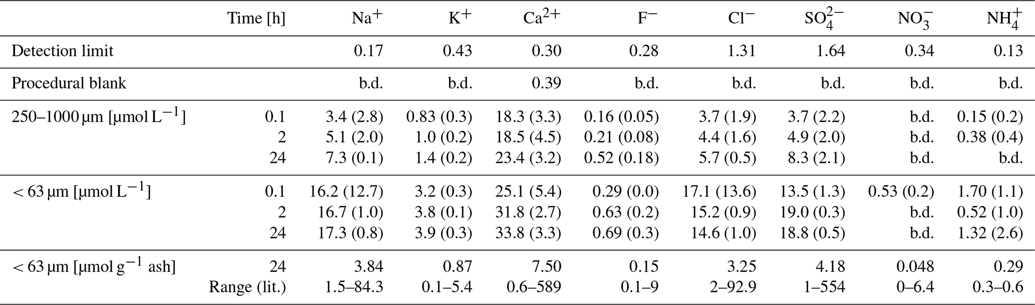
Ion chromatography results for Na⁺, K⁺, Ca²⁺, F⁻, Cl⁻, NO${}_{\mathrm{3}}^{-}$ and SO${}_{\mathrm{4}}^{\mathrm{2}-}$ showed that ion inputs were generally higher in the presence of smaller ash size particles (Table 2), as has been reported previously (Jones and Gislason, 2008; Óskarsson, 1980; Rubin et al., 1994). The leaching from ash components into deionised water occurred almost instantly with limited or no increases in leached concentrations observed between 0, 2 and 24 h (Table 2). For larger particles, there was less release of most ions. In the case of Ca²⁺ and SO${}_{\mathrm{4}}^{\mathrm{2}-}$, a more gradual leaching effect was apparent (Table 2). The concentrations of NO${}_{\mathrm{3}}^{-}$ and NH${}_{\mathrm{4}}^{+}$ were generally below detection suggesting that ash was a minor source of fixed-nitrogen into solution. These observations are consistent with the trends in prior work using a range of volcanic ash and incubation conditions (Duggen et al., 2010; Witham et al., 2005). Major ion analysis was only conducted in deionised water, as no significant changes would be observable for most of these ions in brackish or saline waters under the same conditions.

Table 2 Major ion and macronutrient concentrations in micromoles per litre (µmol L⁻¹) leached from the two size fractions of ash (< 63 and 250–1000 µm) into deionised water (b.d. stands for below detection). Shown are mean values, with the standard deviation in parentheses (n=4). Also shown are mass normalised values (µmol g⁻¹ ash) and a comparison to the range of values reported by Jones and Gislason (2008); the latter is referred to as “Range (lit.)” in the table.

3.4 Trace elements in leach experiments

The release of nanomolar concentrations of dissolved Fe and Mn was evident when ash was resuspended in aged seawater for 10 min (Fig. 6). The net release of dissolved metals proceeded with varying relationships with ash loading over the applied gradient (2–50 mg L⁻¹). Dissolved Mn, Pb, Cu and Co release exhibited significant (p<0.05) positive relationships with ash loading, with Mn and Cu exhibiting the most linear behaviour (R² of 0.99 and 0.83 respectively). Dissolved Fe, Cd and Ni showed no significant relationships with ash loading over the applied range. The initial concentration of metals in South Atlantic seawater should, however, also be considered when interpreting the trends. The magnitude of changes in Cd and Ni concentrations were smallest relative to both the initial concentration and the standard deviation on the initial concentration (0.38 ± 0.04 nM Cd and 6.58 ± 0.76 nM Ni respectively). Thus, it would be difficult to extract a clear relationship irrespective of their chemical behaviour. For other elements (Fe, Co and Pb), non-linearity between ash addition and trace metal concentrations as well as some negative changes in concentrations both likely reflect scavenging of metal ions onto ash particle surfaces (Rogan et al., 2016). Fe, Co and Pb are all scavenged-type elements, and so increasing the surface area of ash present may affect the net change in metal concentration. The divergence between the behaviour of Mn and Fe, with Mn showing a stronger relationship with ash loading, supports the hypothesis of Mendez et al. (2010) that the release of dissolved Mn from aerosols into seawater depends primarily on ash Mn availability, whereas the release of dissolved Fe is more dependent on the nature of organic material present in solution.

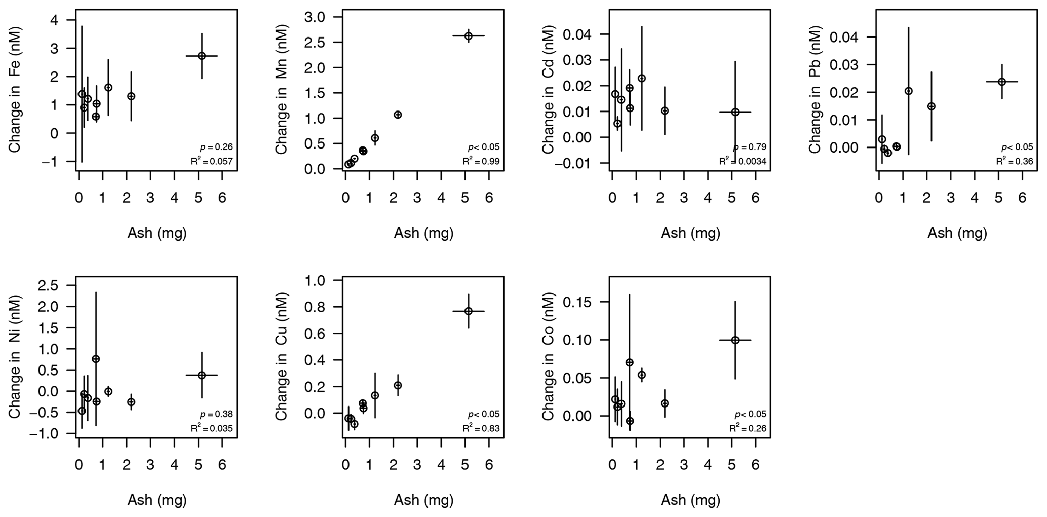
Figure 6 Change in trace metal concentrations after varying ash addition to 100 mL of South Atlantic seawater for a 10 min leach duration at room temperature. Initial (mean ± standard deviation) dissolved trace metal concentrations – deducted from the final concentrations to calculate the change as a result of ash addition – were 0.98 ± 0.03 nM Fe, 0.38 ± 0.04 nM Cd, 13 ± 2 pM Pb, 6.58 ± 0.76 nM Ni, 0.84 ± 0.07 nM Cu, 145 ± 9 pM Co and 0.72 ± 0.05 nM Mn. Error bars are standard deviations from triplicate treatments with similar ash loadings. p values and R² values for a linear regression are annotated. Source data are provided in the Supplement (Table S5). The same data with individual replicates are also shown in the Supplement (Fig. S1).

In addition to the release of dFe in solution, which generally exists as Fe(III) species in oxic seawater (Gledhill and Buck, 2012), the release of Fe(II) was evident on a similar timescale when cold (5–7 ^∘C) aged South Atlantic seawater was used as leachate (Fig. 7). The half-life of Fe(II) decreases more than 10-fold as temperature is increased from 5 to 25 ^∘C, leading to Fe(II) decay on timescales shorter than the time required for analysis (approximately 60 s for solution to enter the flow injection apparatus, mix with reagent and generate a peak) (Santana-Casiano et al., 2005). Elevated Fe(II) concentrations (mean 0.8 nM; Table S2) were evident at this temperature (5–7 ^∘C), which represents an intermediate sea surface temperature for the high-latitude ocean. A sharp decline in Fe(II) dissolution efficiency with increasing ash load was also evident (Fig. 7). Both the highest Fe(II) concentration and the highest net release of Fe(II) were observed at the lowest ash loading (Figs. 7 and S2). The Fe(II) concentration following dust addition into seawater was possibly reduced when the same experimental leaches with ash were repeated 9 months after the initial experiment. The first leaches were conducted ∼ 2 weeks after ash collection. The absence of a clear change between 2 weeks and 4 months precludes an accurate assessment of the rate at which Fe(II) solubility may have decreased.

As Fe(II) concentrations were measured continuously using flow injection analysis, the temporal development of the Fe(II) concentration after ash addition to cold seawater can also be shown (Fig. 7). Considering the set of leach experiments collectively, all ash additions were characterised by a sharp increase in Fe(II) concentrations in the first minute after ash addition into seawater. This was typically followed by a decline and then a relatively stable Fe(II) concentration (Fig. 7).

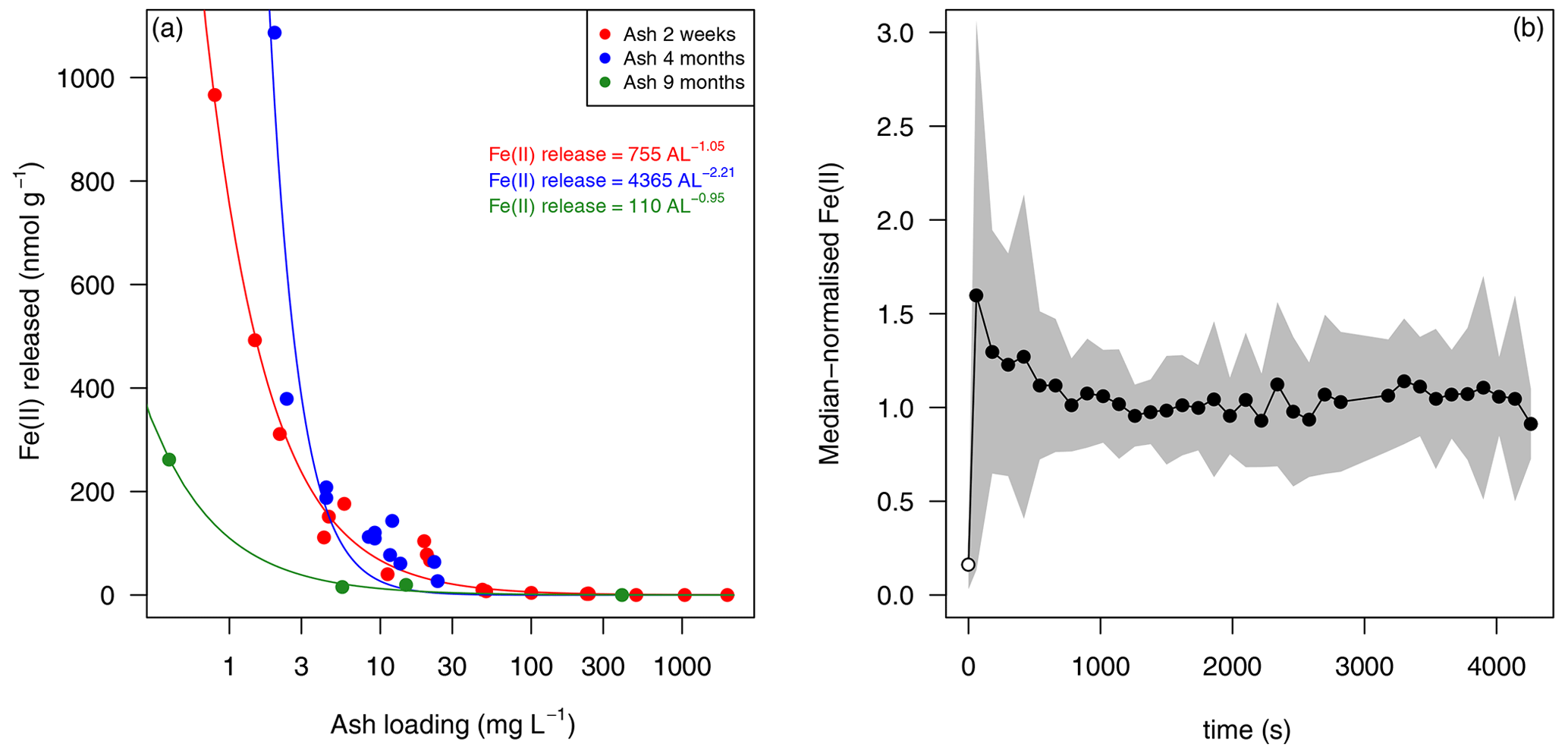
Figure 7 Fe(II) release from Calbuco ash into seawater. (a) Mean Fe(II) released into South Atlantic seawater over a 30 min leach at 5–7 ^∘C. The same batch of Calbuco ash was subsampled and used to conduct experiments on three occasions after the 2015 eruption (2 weeks, 4 months and 9 months since ash collection). The lines are power law fits, with the associated equations shown in the legend. (b) The three time series of Fe(II) concentrations following ash addition are considered collectively by normalising the measured concentrations, such that 1.0 represents the median Fe(II) concentration measured in each experiment. All experiments were conducted for at least 30 min, those conducted with 4- and 9-month-old ash were extended for 1 h. The black line shows the mean response over 34 leach experiments with varying ash loading, and the shaded area shows ± 1 standard deviation. The initial Fe(II) concentration (pre-ash addition at 0 s) in all cases was below detection; thus, the detection limit is plotted at 0 s (open circle). Source data are provided in the Supplement (Table S2).

3.5 Satellite observations

The 5 d composite images of atmospheric aerosol loading (UV aerosol index, which largely represents strongly UV-absorbing dust; Torres et al., 2007) indicated two main volcanic eruption plume trajectories following the major eruptions on 22 and 23 April: (i) northwards over the Pacific, and (ii) northeast over the Atlantic. Daily resolved time series were constructed for regions in the Atlantic and Pacific with elevated atmospheric aerosol loading (UV aerosol index ∼ 2 a.u., arbitrary units; Fig. 8). The Pacific time series indicated a pronounced peak in the aerosol index followed by chlorophyll a 1 d later. A control region to the south of the ash-impacted Pacific region showed no clear changes in chlorophyll a matching that observed in the higher UV aerosol index region to the north (Fig. S3 in the Supplement).

Conversely, in the Atlantic, where the background chlorophyll a concentration was higher throughout the time period of interest, the main area with enhanced aerosol index was not clearly associated with a change in chlorophyll a dynamics on a timescale comparable to that observed following other volcanic-ash-fertilised events (Fig. 8). In a smaller ash-impacted area to the south of the Rio de la Plata (Fig. S3 in the Supplement), where nitrate levels are expected to be higher than to the north and Fe levels also expected to be elevated due its location on the continental shelf, a chlorophyll a peak was evident 7 d after the UV aerosol peak. However, this was not well constrained due to poor satellite coverage in the period after the eruption.

Prior eruptions have been attributed to driving time periods of enhanced regional marine primary production beginning 3–5 d post-eruption (Hamme et al., 2010; Langmann et al., 2010; Lin et al., 2011), and bottle experiments showing positive chlorophyll changes in response to ash addition are typically significant compared with controls within 1–4 d following ash addition (Browning et al., 2014; Duggen et al., 2007; Mélançon et al., 2014).

Figure 8 Potential biological impact of the 2015 Calbuco eruption observed via satellite remote sensing. (a–f) Spatial maps showing the distribution of ash in the atmosphere (UV aerosol index) and corresponding images of chlorophyll a. Images were composited over 5 d periods. Grey lines in the chlorophyll maps correspond to the UV aerosol index = 2 a.u. contour. (g, h) Time series of the UV aerosol index and chlorophyll a for regions of the Pacific (g) and Atlantic (h) oceans, identified by boxes in the maps. Red vertical lines (22 April) indicate the first eruption date. (i) Mean World Ocean Atlas surface NO₃ concentrations. Thin black lines indicate the 500 m bathymetric depth contour.

4 Discussion

4.1 Local drivers of 2015 bloom dynamics in Reloncaví Fjord

The north Patagonian archipelago and fjord region have a seasonal phytoplankton bloom cycle with peaks in productivity occurring in May and October (austral autumn and spring) and the lowest productivity consistently in June (austral winter) (González et al., 2010). Diatoms normally dominate the phytoplankton community during the productive period due to high light availability and high silicic acid supply, both of which are influenced by freshwater runoff (González et al., 2010; Torres et al., 2014). Therefore, the austral autumn season, encompassing the April–May 2015 ash deposition events, is expected to have a high phytoplankton biomass (Iriarte et al., 2007; León-Muñoz et al., 2018) which terminates abruptly with decreasing light availability in austral winter (González et al., 2010).

Whilst not directly comparable, the magnitude of the 2015 bloom in terms of diatom abundance (Fig. 4) was more intense than that reported in Reloncaví Sound for 2001–2008. With respect to the timing of the phytoplankton bloom, the low diatom abundances and chlorophyll a concentrations at the end of May (Fig. 4) are consistent with prior observations of sharp declines in primary production moving into June (González et al., 2010). Peaks in diatom abundance were measured at two stations on 14 May 1 week after the third (small) eruptive pulse, and measured chlorophyll a concentrations were highest close to station C on 30 April (Fig. 4). The high-resolution pH and O₂ data collected at station C from mooring data are consistent with an intense phytoplankton bloom between ∼ 29 April and 7 May (Fig. 3), indicated by a shift to slightly higher pH and O₂ during this time period when river flow into the fjord was stable.

Without a direct measure of ash deposition per unit area in the fjord, turbidity, or higher-resolution chlorophyll or diatom data, it is challenging to unambiguously determine the extent to which the austral autumn phytoplankton bloom was affected by volcanic activity. The high abundance of diatoms at two of three stations sampled could have resulted from ash fertilisation. However, if this was the case, it is not clear which nutrient was responsible for this fertilisation, why the bloom initiation occurred about 1 week after the third eruptive pulse (several weeks after the main eruption events) and the extent to which the timing was coincidental given that productivity normally peaks in May. Reloncaví Fjord was to the south of the dominant ash deposition from the 22 and 23 April eruptions (Romero et al., 2016); thus, ash was delivered by a mixture of vectors including runoff and rainfall. The Petrohué River basin was particularly severely affected by ash with deposition of up to 50 cm of ash in places. This complicates the interpretation of the time series provided by high-resolution data (Fig. 3). With incident light also highly variable over the time series (Fig. 3f), there are clearly several factors, other than volcanic ash deposition, which will have exerted some influence on diatom and chlorophyll a abundance throughout May 2015.

Primary production in the Reloncaví region is thought to be limited by light availability rather than macronutrient availability (González et al., 2010). Whilst micronutrient availability relative to phytoplankton demand has not been extensively assessed in this fjord, with such high riverine inputs across the region – which are normally a large source of dissolved trace elements into coastal waters (e.g. Boyle et al., 1977) – limitation of phytoplankton growth by Fe (or another micronutrient) seems implausible. Reported Fe concentrations determined by a diffusive gel technique in Reloncaví Fjord in October 2006 were relatively high: 46–530 nM (Ahumada et al., 2011). Similarly, reported dFe concentrations in the adjacent Comau Fjord at higher salinity are generally in the nanomolar range and remain > 2 nM even under post-bloom conditions which suggests that dFe is not a limiting factor for phytoplankton growth (Hopwood et al., 2020; Sanchez et al., 2019).

Silicic acid availability could have been increased by ash deposition. Whilst not quantified herein, an increase in silicic acid availability from ash in a region where silicic acid was suboptimal for diatom growth could plausibly explain higher than usual diatom abundance (Siringan et al., 2018). Silicic acid concentrations were indeed high (up to 118 µM) in Reloncaví Fjord surface waters and > 30 µM at 15 m depth (salinity 33.4) (Vergara-Jara et al., 2019; Yevenes et al., 2019). However, concentrations > 30 µM are typical during periods of high runoff and, accordingly, are not thought to limit primary production or diatom growth in this area (González et al., 2010). The Si(OH)₄ : NO₃ ratio in Reloncaví Fjord and downstream Reloncaví Sound also indicates an excess of Si(OH)₄, with ratios of approximately 2:1 observed in fjord surface waters throughout the year (González et al., 2010; Yevenes et al., 2019). For comparison, the ratio of Si : N for diatom nutrient uptake is 15:16 (Brzezinski, 1985). Furthermore, experimental incubations with additions of macronutrients to fjord waters in Reloncaví and adjacent fjords have found strong responses of phytoplankton to additions of silicic acid only when Si(OH)₄ and NO₃ were added in combination, further corroborating the hypothesis that an excess of silicic acid is normally present in surface waters of these fjord systems (Labbé-Ibáñez et al., 2015). Therefore, it is doubtful that changes in nutrient availability from ash alone could explain such high diatom abundances in mid-May.

Alternative reasons for high diatom abundances in the absence of a chemical fertilisation effect are plausible and could include, for example, ash having reduced zooplankton abundance or virus activity in the fjord, thereby facilitating higher diatom abundance than would otherwise have been observed by decreasing diatom mortality rates in an environment where nutrients were replete. The role of volcanic ash in driving such short-term ecological shifts in the marine environment is almost entirely unstudied (Weinbauer et al., 2017). However, volcanic ash deposition of 7 mg L⁻¹ in lakes within this region during the 2011 Puyehue-Cordón Caulle eruption was reported to increase post-deposition phytoplankton biomass and decrease copepod and cladoceran biomass (Wolinski et al., 2013). The proposed mechanism was ash particle ingestion negatively affecting zooplankton, and ash-shading positively affecting phytoplankton via reduced photoinhibition (Balseiro et al., 2014; Wolinski et al., 2013).

Considering the more modest peak in diatom abundance at the most strongly ash-affected station (station A, Fig. 4) and the timing of the peak diatom abundance 3 weeks after the main eruption, it is clear that the interaction between ash and phytoplankton in the Reloncaví Fjord was more complex than the simple Fe fertilisation proposed for the southeast Pacific (Fig. 8g). In the absence of an immediate diatom fertilisation effect from Fe or silicic acid, we hypothesise that any change in phytoplankton bloom dynamics within Reloncaví Fjord was mainly a “top-down” effect driven by the physical interaction of ash and different ecological groups in a nutrient-replete environment, rather than a “bottom-up” effect driven by the alleviation of nutrient limitation from ash dissolution.

4.2 Volcanic ash as a unique source of trace elements

The release of the bio-essential elements Fe and Mn from ash here ranged from 53 to 1200 (dFe) and from 48 to 71 nmol g⁻¹ (dissolved Mn). For dFe, this is comparable to the rates determined in other studies under similar experimental conditions for subduction zone volcanic ash, with reported Fe release in prior work ranging from 2 to 570 nmol g⁻¹ (Table S1 in the Supplement). For Mn, less prior work is available, but these values are within the 17–1300 nmol g⁻¹ range reported by Hoffmann et al. (2012). Fe(II) release was particularly efficient at ash loadings < 5 mg L⁻¹ (Fig. 7), whereas dFe release was less sensitive to ash loading (Fig. 6). The timing of Fe(II) release in the first 60 s of incubations suggests a fast dissolution process. Fe(II) is short-lived in oxic surface seawater with an observed half-life of only 10–20 min even in the Southern Ocean where cold surface waters slow Fe(II) oxidation (Sarthou et al., 2011). However, relative to Fe(III), Fe(II) is also more soluble and, from an energetic perspective, expected to be more bio-accessible to cellular uptake (Sunda et al., 2001). Whilst it is known that the vast majority of dFe leached from ash into seawater tends to occur in the first minutes of ash addition (Duggen et al., 2007; Jones and Gislason, 2008), and this could be consistent with rapid dissolution of highly soluble phases on ash surfaces, we note that there is not yet conclusive evidence concerning the precise origin of this dFe pulse. Fe(II) salts may be present on the surface of ash particles (Horwell et al., 2003; Hoshyaripour et al., 2015); thus, the Fe(II) observed herein (Fig. 7) may reflect almost instantaneous release following the dissolution of thin layers of salt coatings in ash surfaces (Ayris and Delmelle, 2012; Delmelle et al., 2007; Olsson et al., 2013). Alternatively Fe(II) could be released from more crystalline Fe(II) phases. Prior work, at much lower pH (pH 1 H₂SO₄ representing conditions that ash surfaces may experience during atmospheric processing, although not in aquatic environments) suggests that the short-term release of Fe(II) or Fe(III) is determined by the surface Fe(II) : Fe ratio which may differ from the bulk Fe(II) : Fe ratio due to plume processing (Maters et al., 2017).

Different leaching protocols are widely recognised as a major challenge for interpreting and comparing different dissolution experiment datasets for all types of aerosols (Duggen et al., 2007; Morton et al., 2013). When Fe(II) is released into solution as a considerable fraction of the total dFe release, this is particularly challenging to monitor, as Fe(II) oxidises on timescales of seconds to minutes depending on temperature, pH and O₂ conditions (Santana-Casiano et al., 2005). The dFe and Fe(II) leaching protocols used herein are only comparable qualitatively, as the Fe(II) method using cooler seawater and larger seawater volumes was specifically designed to test for the presence of rapid Fe(II) release and to evaluate the short-term temporal trend of any such release. However, for rough comparative purposes, the Fe(II) released was equivalent to 38 ± 25 % (mean ± standard deviation) of the dFe released at ash loadings from 1 to 10 mg L⁻¹ and 19 ± 17 % of the dFe for ash loadings from 10 to 50 mg L⁻¹. These values are reasonably comparable to the 26 % median Fe(II) : dFe fraction measured in Fe released into seawater from aerosols collected across zonal transects of the Pacific Ocean (Buck et al., 2013), suggesting that fresh Calbuco ash is roughly comparable in terms of Fe(II) lability to these environmentally processed aerosols.

4.3 A potential fertilisation effect in the southeast Pacific

Experiments with ash suspensions have shown that ash loading has a restricted impact on satellite chlorophyll a retrieval (Browning et al., 2015), thereby offering a means to assess the potential biological impact of the 2015 Calbuco eruption in offshore waters. We found evidence for fertilisation of offshore Pacific seawaters in the studied area (Fig. 8). Following the eruption date, mean chlorophyll a concentrations increased ∼ 2.5 times over a broad region where the elevated UV aerosol index was detected (Fig. 8g). Both the timing and location of this chlorophyll a peak were consistent with ash fertilisation, with the peak of elevated chlorophyll a being located within the core of the highest atmospheric aerosol loading, and the peak date occurring 1 d after the main passage of the atmospheric aerosol plume. A similar phytoplankton response time frame was reported following ash deposition in the northeast Pacific following the August 2008 Kasatochi eruption (Hamme et al., 2010) which was similarly thought to be triggered by the relief of Fe limitation (Langmann et al., 2010). At the same time, a control region to the south of the ash-impacted Pacific region showed no clear changes in chlorophyll a matching that observed in the higher UV aerosol index region to the north (Fig. S3 in the Supplement).

In the southwest Atlantic, two ash-impacted areas are highlighted: one to the north (Fig. 8) and one to the south of the Rio de la Plata (Fig. S3 in the Supplement). Nitrate levels are expected to be higher in the south than in the north, with Fe levels expected to be elevated across both locations as a result of their position on the continental shelf. In the area to the north of the Rio de la Plata (Fig. 8), ash deposition indicated by the UV aerosol index did not lead to such a clear corresponding change in chlorophyll a concentrations (Fig. 8h), although it is not possible to rule out the possibility of fertilisation completely with the available data (e.g. whilst also being proceeded by a larger chlorophyll a peak on 21 April, there is a peak in chlorophyll a at 25 April coinciding with elevated UV aerosol index). Phytoplankton growth in this region of the Atlantic is expected to be limited by fixed nitrogen availability, as a result of strong stratification (Moore et al., 2013); thus, dFe release from ash particles alone would not be expected to result in short-term increases to primary production. In the second area of ash deposition, to the south (Fig. S3 in the Supplement), a chlorophyll a peak was evident 7 d after the UV aerosol peak. However, this was not well constrained due to poor satellite coverage in the period after the eruption. Considering the dynamic spatial and temporal variation in chlorophyll within this coastal area, it is challenging to associate any change in chlorophyll specifically with ash arrival.

The change in chlorophyll a observed in the southeast Pacific contrasts with results in Reloncaví Fjord, where phytoplankton abundances likely peaked much later than the first ash arrival – after 28 April. The fertilised region of the Pacific (Fig. 8) hosts upwelling of deep waters, supplying nutrients in ratios that are deficient in dFe (Bonnet et al., 2008; Torres and Ampuero, 2009). Fe limitation of phytoplankton growth in this region is therefore anticipated, which could have been temporarily relieved following ash deposition and dFe release (Fig. 6). Thus, the differential responses observed in the Pacific and Atlantic are consistent with the anticipated nutrient-limitation regimes (Fe limited and nitrogen limited respectively) and the supply of dFe but not fixed N (NO₃ or NH₄) from the Calbuco ash (Fig. 6 and Table 2).

5 Conclusions

The contrasting effects of volcanic ash on primary producers in Reloncaví Fjord, the southeast Pacific and southwest Atlantic oceans support the hypothesis that the response of primary producers is dependent on both the ash loading and the resources limiting primary production in a region at a specific time of year. Leach experiments using ash from the 2015 Calbuco eruption demonstrated a small increase in the alkalinity of deionised water from fine but not coarse ash as well as no significant addition of fixed nitrogen (quantified as NO₃ and NH₄) into solution. In saline waters, the release of dissolved trace metals including Mn, Cu, Co, Pb, Fe and specifically Fe(II) was evident.

Strong evidence of a broad-scale “bottom-up” fertilisation effect of ash on phytoplankton was not found locally within Reloncaví Fjord, although it is possible that the timing and peak diatom abundance of the autumn phytoplankton bloom may have shifted in response to high ash loading in the weeks following the first eruption. High diatom abundances at some stations within the fjord several weeks after the eruption may have arisen from a “top-down” effect of ash on filter-feeders, although the mechanism can only be speculated herein. No clear positive effect of ash deposition on chlorophyll a was evident in the southwest Atlantic, consistent with expected patterns in nutrient deficiency which suggest the region to be nitrogen limited. However, in offshore waters of the southeast Pacific where Fe is anticipated to limit phytoplankton growth, a chlorophyll a increase was related to maximum ash deposition, and we presume that this increase in chlorophyll a was likely driven by Fe fertilisation.