Imprint of chaotic ocean variability on transports in the southwestern Pacific at interannual timescales

The southwestern Pacific Ocean sits at a bifurcation where southern subtropical waters are redistributed equatorward and poleward by different ocean currents. The processes governing the interannual variability of these currents are not completely understood. This issue is investigated using a probabilistic modeling strategy that allows disentangling the atmospherically forced deterministic ocean variability and the chaotic intrinsic ocean variability. A large ensemble of 50 simulations performed with the same ocean general circulation model (OGCM) driven by the same realistic atmospheric forcing and only differing by a small initial perturbation is analyzed over 1980–2015. Our results show that, in the southwestern Pacific, the interannual variability of the transports is strongly dominated by chaotic ocean variability south of 20^∘ S. In the tropics, while the interannual variability of transports and eddy kinetic energy modulation are largely deterministic and explained by the El Niño–Southern Oscillation (ENSO), ocean nonlinear processes still explain 10 % to 20 % of their interannual variance at large scale. Regions of strong chaotic variance generally coincide with regions of high mesoscale activity, suggesting that a spontaneous inverse cascade is at work from the mesoscale toward lower frequencies and larger scales. The spatiotemporal features of the low-frequency oceanic chaotic variability are complex but spatially coherent within certain regions. In the Subtropical Countercurrent area, they appear as interannually varying, zonally elongated alternating current structures, while in the EAC (East Australian Current) region, they are eddy-shaped. Given this strong imprint of large-scale chaotic oceanic fluctuations, our results question the attribution of interannual variability to the atmospheric forcing in the region from pointwise observations and one-member simulations.

1 Introduction

The southwestern Pacific Ocean is a region comprising many islands, seamounts and reefs. The interactions between the large-scale oceanic currents and the complex bathymetry lead to a complex set of oceanic currents (Fig. 1) transporting mass, heat and water properties, as well as connecting the various habitats and ecosystems across the Coral Sea and Tasman Sea, with different connectivity for different oceanic depths (Ceccarelli et al., 2013). As a mean, the large-scale westward South Equatorial Current (SEC) enters the Coral Sea where it divides into westward zonal jets when encountering the islands of Fiji, the Vanuatu Archipelago and New Caledonia (Kessler and Cravatte, 2013a; Couvelard et al., 2008; Qu and Lindstrom, 2002). These westward zonal jets flow to the Australian coast, where they bifurcate northward toward the Solomon Sea, feeding the low-latitude western boundary currents (LLWBCs) and the equatorial current system downstream. They also bifurcate southward, feeding the East Australian Current (EAC). South of New Caledonia located around 22^∘ S, the shallow STCC (Subtropical Countercurrent) flows eastward above the westward subsurface SEC. The region is characterized by a relatively high eddy kinetic energy level (Qiu and Chen, 2004; Qiu et al., 2009), strongly sheared mean currents and vigorous western boundary currents; the presence of islands favors the generation of instabilities and mesoscale eddies (Qiu et al., 2009; Keppler et al., 2018; Rieck et al., 2018; Travis and Qiu, 2017).

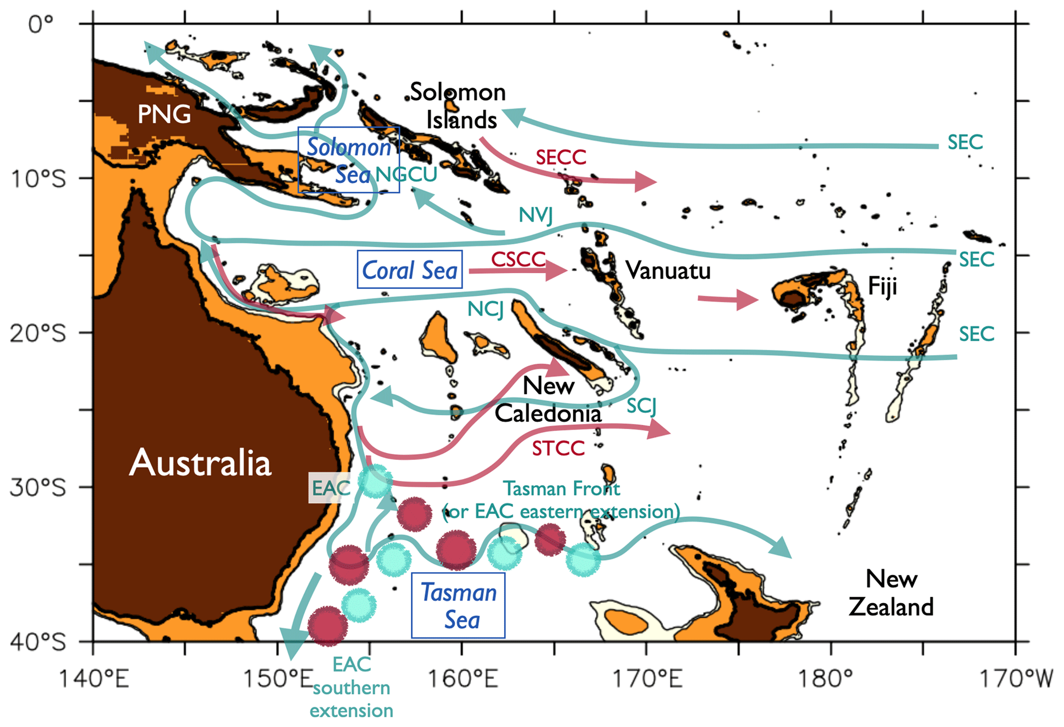
Figure 1 Reference map of the southwestern Pacific, with the names of the main islands and countries, and a schematic of the subsurface circulation (top 1000 m, green arrows) and surface circulation, shown when different from the subsurface (red arrows). Brown and orange shading shows bathymetry at depths of 500 and 1000 m. PNG: Papua New Guinea. Indicated are the branches of the SEC (South Equatorial Current), the NVJ (North Vanuatu Jet), the NCJ and SCJ (North and South Caledonian Jet), the STCC (Subtropical Countercurrent), EAC (East Australian Current), NGCU (New Guinea Coastal Undercurrent), and the SECC (South Equatorial Countercurrent). The red and green circles are schematics for the eddy field. The map is based on previous literature, in particular Ganachaud et al. (2004) and Oke et al. (2019a).

Understanding the variability of the various current transports in the region is of key importance to better predict the variability of the mass, heat and freshwater transports and the water mass connections, with implications for the climate. The currents in the whole southwestern Pacific have been shown to vary at various timescales, with a dominant intraseasonal component linked to the presence of mesoscale eddies (Qiu and Chen, 2004; Qiu et al., 2009; Cravatte et al., 2015). At seasonal timescales, the 0–1000 m large-scale transports are driven by the spin-up and spin-down of the subtropical gyre (Kessler and Gourdeau, 2007). The interannual variability of zonal and meridional currents transports has been less documented and is the focus of the present study.

On interannual timescales, the regional currents (and hence transports) are impacted by two main climate modes. The first is the El Niño–Southern Oscillation (ENSO), the dominant mode of interannual variability in the tropical band with remote oceanic and atmospheric teleconnections (see Sprintall et al., 2020 for a review). The second, farther south in the extratropics, is the Southern Annular Mode (SAM) (Thompson and Wallace, 2000). The latter is characterized by meridional shifts in westerly wind stress, potentially influencing the transports at midlatitudes. On decadal scales, wind anomalies in the Southern Hemisphere have also been shown to impact sea surface height and eddy kinetic energy (EKE) (Hill et al., 2008; Cai, 2006; Holbrook et al., 2005, 2011).

Through its dipole signature in wind stress curl anomalies in the southern Pacific from the Equator to about 25^∘ S, ENSO causes large-scale sea surface height (Zilberman et al., 2013) and transport anomalies. Through the propagation of Rossby waves, the transport anomalies in the western Pacific are affected by these anomalies integrated over the basin. The total 0–1000 m zonal transport of waters entering the Coral Sea between New Caledonia and Solomon Islands is reduced a few months after a La Niña and increases a few months after an El Niño, depending on the El Niño flavor (Kessler and Cravatte, 2013b). ENSO modulates the meridional transport (e.g., Ishida et al., 2008; Lee and Fukumori, 2003) and the LLWBC flowing into the Solomon Sea in the upper layer accordingly (Melet et al., 2013; Davis et al., 2012; Kessler et al., 2019).

In contrast, south of ∼25^∘ S, only a small fraction of the EAC transport variability at interannual timescales has been attributed to ENSO (Ridgway, 2007; Cetina-Heredia et al., 2014). At these latitudes, the ENSO-related wind stress curl anomalies are weaker, and remote action by such curl-generated Rossby waves is hampered by the several years it takes for those to propagate from the forcing region to the western part of the basin: the ocean thus acts as a low-pass filter for ENSO-induced variations (Sasaki et al., 2008). The SAM, however, exhibits stronger wind stress curl anomalies close to the western boundary, forcing simultaneous increases in the EAC strength and recirculation-induced meridional transports across 32^∘ S during the SAM positive phase (Zilberman et al., 2014).

In the 15–30^∘ S band encompassing the STCC region, the processes governing the interannual variability of the various currents are unclear. A previous attempt to explain this variability found inconsistent interannual transport variations in the region between two oceanic simulations (OFAM3 (Ocean Forecasting Australia Model) at $\mathrm{1}/\mathrm{10}$^∘ and ROMS (Regional Oceanic Modeling System) at $\mathrm{1}/\mathrm{12}$^∘ spatial resolutions) driven by the same atmospheric forcing (J. Clary, unpublished results) and observations. This suggests that the previous large-scale atmospheric interannual modes may not be the main drivers of the transport interannual variability in the region and that other mechanisms must be invoked to explain this variability.

In particular, recent studies have highlighted the importance of nonlinear internal ocean dynamics in spontaneously generating interannual variability, which is substantial in eddy-active regions (e.g., Penduff et al., 2011; Sérazin et al., 2015). This so-called intrinsic variability, which can be strong and more importantly has a random phase, can imprint on large-scale and integrated quantities such as the ocean heat content (Sérazin et al., 2017; Penduff et al., 2018) and the volume transport of the overturning circulation (Grégorio et al., 2015; Leroux et al., 2018; Jamet et al., 2020). Regarding those results, the ocean appears to be a chaotic system that is partly paced by the atmosphere and whose nonlinearities induce a sensitivity to small perturbations (Zanna et al., 2018). This supports the need for ensemble ocean simulations to characterize the forced and intrinsic variabilities (e.g., Penduff et al., 2014; Bessières et al., 2017).

Mesoscale eddies, whose evolution is largely chaotic, are ubiquitous in the region south of about 20^∘ S (Keppler et al., 2018), and the current variability at intraseasonal timescales is much larger than at interannual timescales (Qiu and Chen, 2004; Qiu et al., 2009; Cravatte et al., 2015). Sérazin et al. (2015) also show that interannual intrinsic variability is important in this region, suggesting a nonlinear upscaling from mesoscale fluctuations towards low frequencies: nonlinear dynamics, including baroclinic instability, scale interactions and rectification (e.g., Sérazin et al. 2018; Zanna et al., 2018), may be strong enough to eventually generate intrinsic interannual variability (Belmadani et al., 2017; Davis et al., 2014). Therefore, it is plausible that some of the interannual variability arises from the intrinsic ocean variability alone.

The aim of this paper is to test this latter hypothesis and to evaluate the respective parts of the external atmospheric variability and of the chaotic oceanic processes in driving the interannual variability of the transports in the whole southwestern Pacific. For that purpose, a probabilistic modeling strategy is used: an ensemble of 50 global $\mathrm{1}/\mathrm{4}$^∘ ocean–sea ice simulations, driven by the same realistic atmospheric forcing over 1960–2015 and differing only by slightly perturbed initial conditions (Penduff et al., 2014), is analyzed over 1980–2015 to interpret the current interannual variability.

This oceanic ensemble simulation was performed in the framework of the OCCIPUT (OceaniC Chaos – Impacts, strUcture, predicTability) project and has already been used to show that internal oceanic dynamics can spontaneously generate substantial variability over a wide temporal spectrum, including interannual, decadal and long-term trends (Gregorio et al., 2015; Leroux et al., 2018; Penduff et al., 2018, 2019; Serazin et al., 2016; Llovel et al., 2018). The oceanic variability that is deterministically driven by the prescribed atmospheric variability (e.g., containing the ENSO or SAM atmospheric signal) is estimated from the ensemble mean evolution. Some of the prescribed atmospheric forcing may also originate from chaotic behavior in the coupled system. However, as we focus on the ocean, we will use the term “deterministic” to characterize the variability in the ocean common to all simulations. The intrinsic oceanic variability is then quantified from the random dispersion of the 50 members around the ensemble mean. To characterize this variability arising from ocean internal processes, we will use the term “chaotic” in the rest of the paper. The results obtained with this modeling approach will help us to understand the processes governing the interannual variability in the 15–30^∘ S area, which is not well documented, and will allow us to revisit the conclusions of previous studies on transport and EKE deterministic forcing.

Section 2 describes the ensemble of simulations used and how deterministic and chaotic variability is quantified. It also describes the data used for validation. Section 3 quantifies the deterministic and chaotic interannual variability of the 0–1000 m transports and EKE in the southwestern Pacific, with a focus on key main currents. Section 4 investigates the drivers of deterministic variability, while Sect. 5 explores the spatial patterns of oceanic chaotic variability. We show that there are large parts of the region where interannual transport variability is firstly driven by internal chaotic ocean processes, which probably arise from a rectification of the lower-frequency signal by mesoscale activity. This important role played by ocean-only dynamics may thus hamper our capability to identify the atmospheric drivers of the oceanic interannual variability in the southwestern Pacific and thus to predict their behavior at interannual timescales. This has strong implications for the observing systems, as discussed in Sect. 6.

2 Data, model description and methods

2.1 Model simulations and post-processing

The OCCIPUT ensemble is made of 50 global ocean–sea ice hindcasts run for 56 years (1960–2015). The model used is NEMO (Madec, 2008), implemented with a $\mathrm{1}/\mathrm{4}$^∘ spatial resolution and 75 vertical levels (47 levels in the first 1000 m). Model parameters (numerical schemes, subgrid-scale parameterizations) are described in Bessières et al. (2017). At the lateral boundaries, a free-slip boundary condition is applied.

Each simulation is forced by the realistic Drakkar Forcing Set (DFS) version 5.2 based on the ERA-40 and ERA-Interim reanalyses (Dussin et al., 2016). After a 21-year common spin-up (Leroux et al., 2018), the 50 members of the ensemble are generated in 1960 by activating a small stochastic perturbation in the equation of state within each member (Brankart et al., 2015; Bessières et al., 2017). The small perturbations simulate the unresolved fluctuations of potential temperature and salinity. These fluctuations are generated using random walks (see Brankart et al., 2015, for details). The initial perturbations are applied within each member for only 1 year in 1960: they are purely stochastic. As heat fluxes are computed using bulk formulae, they are slightly different in the 50 members because of sea surface temperature (SST) differences. Wind stresses are computed using absolute winds, without ocean current feedbacks, and are thus identical in each of the members. We focus our analyses on the 1980–2015 period; before 1980 indeed, the buoyancy fluxes derived from the DFS5.2 forcing are devoid of interannual variability. Starting our analyses in 1980 thus yields an effective spin-up time of 41 years within each member.

It is important to recall that the perturbations introduced in the members are random by construction and that the 50 realizations of intrinsic variability that emerge from these perturbations are and remain out of phase among the members as well as out of phase with the prescribed atmospheric variability.

The 4D fields of temperature and velocity used in this study are available as monthly means within each member. In addition, temperature and velocity 5 d averages are also available at specific depths for each member. In this study, we focus mainly on two quantities: the 0–1000 m integrated transports and the EKE at the surface and at 100 m. The data processing is done as follows.

• The 0–1000 m integrated zonal and meridional currents are computed from monthly velocities for each member. We call these quantities “vertically integrated transport”, and their unit is m² s⁻¹.

• Long-term trends (very low-frequency signals) are then computed and removed from each time series within each member. This is done using a nonlinear, second-order local regression method (LOESS; Cleveland and Devlin 1988), which high-pass-filters time series with a 9-year cutoff period. This method preserves the length of original time series without adverse edge effects (see Serazin et al., 2015).

• Detrended transport time series are then low-pass-filtered with a 25-month Hanning filter in order to isolate the interannual variability (such a filter eliminates all variability at periods lower than 1 year). Our processing thus confines our analyses and results to timescales between 1 and 9 years.

We also use the 5 d zonal and meridional velocities at the surface and at 100 m depth, high-pass-filtered at periods lower than 180 d with a Hanning filter, to compute the EKE. EKE monthly anomalies from the mean monthly climatology are then computed, and the long-term trend is removed with a linear trend. Detrended time series are then low-pass-filtered with a 25-month Hanning filter to isolate the interannual EKE modulation.

2.2 Estimation of the forced and intrinsic variability

For a given monthly quantity f in member i, we define for each time step t

$$\begin{array}{}\text{(1)}& {\displaystyle }{\displaystyle }{f}_i^{\prime }\left(t\right)=f_i\left(t\right)-f^{\ast }\left(t\right),\end{array}$$

where $f^{\ast }\left(t\right)=\frac{\mathrm{1}}{N}{\sum }_{i=\mathrm{1}}^{i=N}{f}_i\left(t\right)$ is the ensemble mean of the N=50 members (i.e., the atmospherically forced component), and $f_i^{\prime }\left(t\right)$ is the deviation from the ensemble mean (i.e., the oceanic chaotic component).

For the low-pass-filtered signals F in member i, we similarly define for each time step t

$$\begin{array}{}\text{(2)}& {\displaystyle }{\displaystyle }{F}_i^{\prime }\left(t\right)=F_i\left(t\right)-F^{\ast }\left(t\right).\end{array}$$

The intensity of the monthly forced variability is estimated with the variance of the ensemble mean time series, with the bar denoting the time average:

$$\begin{array}{}\text{(3)}& {\displaystyle }{\displaystyle }{\mathit{\sigma }}_F^{\mathrm{2}}={\displaystyle \frac{\mathrm{1}}{(T-\mathrm{1})}}{\sum }_{t=\mathrm{1}}^{t=T}{\left(f^{\ast }\left(t\right)-\stackrel{\mathrm{‾}}{f^{\ast }\left(t\right)}\right)}^{\mathrm{2}}.\end{array}$$

The intensity of the interannual forced variability is estimated with the variance of the ensemble mean time series F^∗(t) low-pass-filtered as explained above:

$$\begin{array}{}\text{(4)}& {\displaystyle }{\displaystyle }\mathit{\sigma }{\text{LF}}_F^{\mathrm{2}}={\displaystyle \frac{\mathrm{1}}{(T-\mathrm{1})}}{\sum }_{t=\mathrm{1}}^{t=T}\left(F^{\ast }\right(t)-\stackrel{\mathrm{‾}}{F^{\ast }\left(t\right)}{)}^{\mathrm{2}}.\end{array}$$

The intensity of the interannual variability induced by chaotic oceanic motions is estimated by the time mean of the ensemble variance (computed from the deviation of each member from the ensemble mean) deduced from the low-pass-filtered time series $F_i^{\prime }\left(t\right)$:

$$\begin{array}{}\text{(5)}& {\displaystyle }{\displaystyle }\mathit{\sigma }{\text{LF}}_I^{\mathrm{2}}=\stackrel{\mathrm{‾}}{{\displaystyle \frac{\mathrm{1}}{(N-\mathrm{1})}}{\sum }_{i=\mathrm{1}}^N\left(F_i^{\prime }\right(t){)}^{\mathrm{2}}},\end{array}$$

where N=50 is the number of ensemble members.

Finally, we define the deterministic variance ratio $R_{\text{LF}}=\mathrm{100}\times \mathit{\sigma }{\text{LF}}_F^{\mathrm{2}}/(\mathit{\sigma }{\text{LF}}_I^{\mathrm{2}}+\mathit{\sigma }{\text{LF}}_F^{\mathrm{2}}$), i.e., the deterministic variance as a percentage of the total variance in each member (see Leroux et al., 2018, Eq. 8). If this ratio is greater than 50 %, the deterministic variance dominates the total variance of the signal.

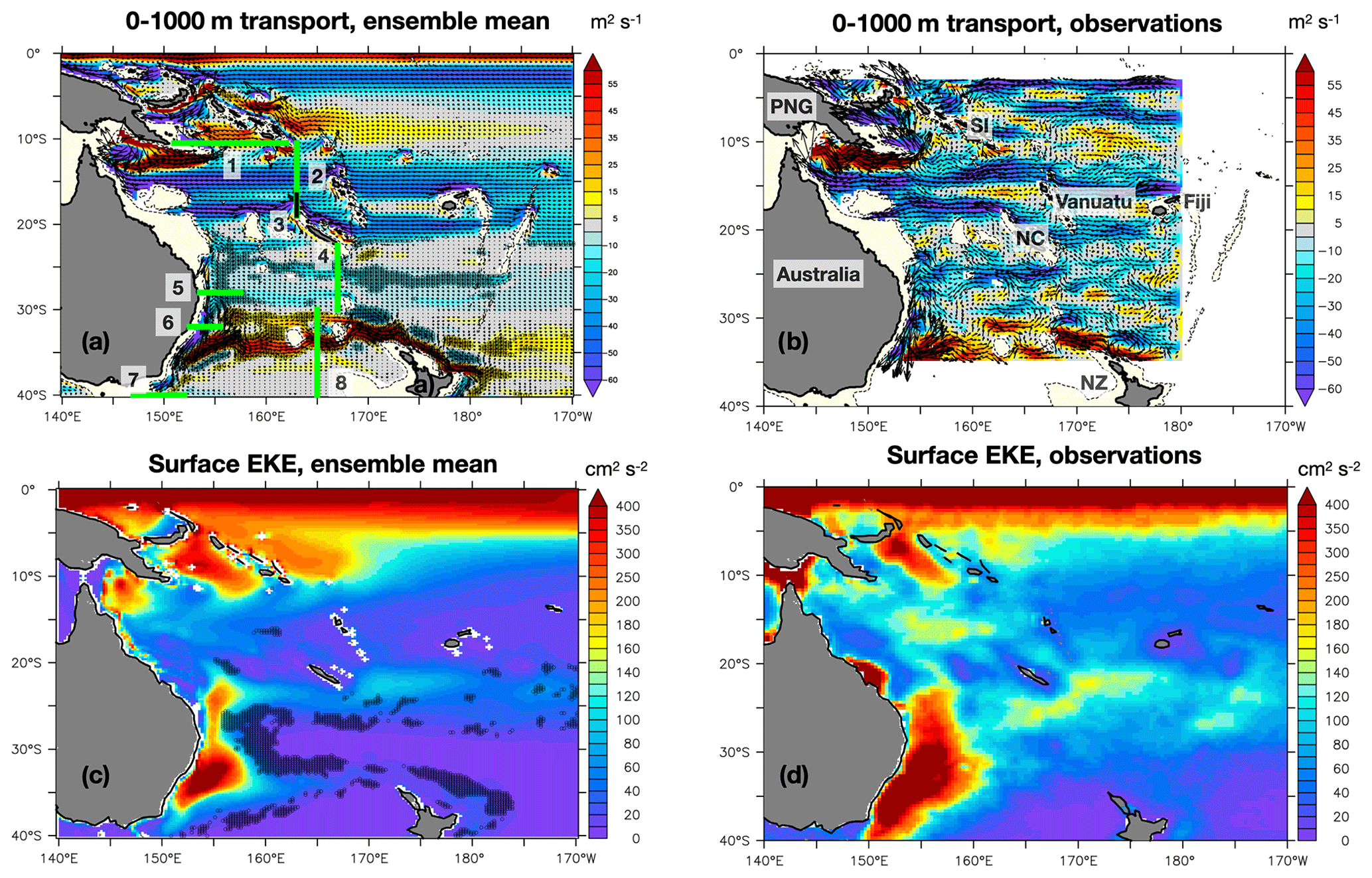
Figure 2 (a) The 1980–2015 time-averaged 0–1000 m transport from the ensemble mean. Colors show zonal transport (positive values mean eastward, negative values westward), and arrows show total transport. The hatched areas show regions where the spread of the 1980–2015 time-averaged 0–1000 m transport is at least 15 % of the ensemble mean. The thick green lines (and the thick black line) show the main current sections shown in Fig. 4, with the associated numbers corresponding to the caption of Fig. 4. (b) 0–1000 m transport from the Argo-Merged observations; colors show zonal transport. The names of the main islands are also indicated. NC: New Caledonia; NZ: New Zealand; SI: Solomon Islands and PNG: Papua New Guinea. (c) Time-averaged ensemble mean of the 1980–2015 surface EKE. The hatched areas show regions where the spread of the 1980–2015 EKE is between 10 % and 20 % of the ensemble mean. (d) 1993–2015 time-averaged surface EKE from the OSCAR product.

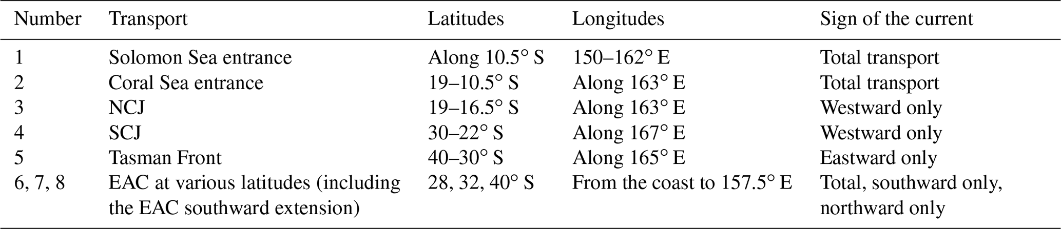
Table 1 Computation of the 0–1000 m transport of key currents shown in Fig. 4. The numbers correspond to the sections shown in Fig. 2.

The interannual variances and the R_LF ratio depend on the spatial scales considered (Serazin et al., 2015). At a model grid point, they are greater than for a field first averaged over a spatial area (see Sect. 3). Both pointwise and regional diagnoses will be presented; the first diagnosis is for quantifying the chaotic variance and deterministic variance ratio in the framework of in situ data comparison, and the second one is for more climate-relevant quantities.

2.3 Estimation of key current transports

In each member, the 0–1000 m transports of key currents are computed as follows (see Fig. 2 and Table 1 for a summary).

• The transport entering the Solomon Sea is computed by integrating the 0–1000 m meridional transport from coast to coast between 150 and 162^∘ E along 10.5^∘ S (labeled 1 in Fig. 2a).

• The transport entering the Coral Sea is computed by integrating the 0–1000 m zonal transport along 163^∘ E from northern tip of New Caledonia to the Solomon Islands (labeled 2 in Fig. 2a).

• The transport of the North Caledonian Jet (NCJ) is computed by integrating the 0–1000 m westward-only zonal transport along 163^∘ E from 19^∘ S (the northern tip of New Caledonia's reef) to 16.5^∘ S (labeled 3 in Fig. 2a); the transport of the South Caledonian Jet (SCJ) is computed by integrating the 0–1000 m westward-only zonal transport along 167^∘ E from 22.5^∘ S (at the southern tip of New Caledonia's reef) to 30^∘ S (labeled 4 in Fig. 2a).

• The Tasman Front transport is computed by integrating the 0–1000 m eastward-only zonal transport along 165^∘ E from 40 to 30^∘ S (labeled 8 in Fig. 2a).

• For the EAC at various latitudes (labeled 5 to 7 in Fig. 2a), in addition to the southward flow only, the net transport of the southward flow and the northward adjacent recirculation are computed following Zilberman et al. (2018): the net transport is computed by integrating the meridional 0–1000 m velocity from the coast to the offshore edge of the southward flow and eastward to the northward EAC recirculation edge located west of 157.5^∘ E. The total EAC transport is also computed and shown. Intrinsic variability for both of these estimates is also given.

2.4 Other datasets

To validate the model outputs, we use a mean absolute geostrophic velocity product based on geostrophic shear estimated from the CARS climatological hydrographic atlas (Ridgway et al., 2002; Condie and Dunn, 2006) (http://www.marine.csiro.au/~dunn/cars2009/index.html, last access: 9 March 2021) and a 1000 m absolute velocity field based on Argo float drift (Kessler and Cravatte, 2013a). These 3D zonal and meridional currents are referred to as “Argo-Merged”.

We also use the OSCAR (Ocean Surface Current Analysis Real-time) near-surface ocean current estimates (Bonjean and Lagerloef, 2002) from 1993 to 2015. Data are on a $\mathrm{1}/\mathrm{3}$^∘ grid with a 5 d resolution. The horizontal currents are directly estimated from sea surface height, the surface vector wind and sea surface temperature. The OSCAR surface current is representative of the top 30 m of the upper ocean.

Finally, we use the Nino3.4 index, defined as the average of the SST anomalies in the 5^∘ S–5^∘ N, 170–120^∘ W box, from the HadISST dataset (Rayner et al., 2003) and the PDO (Pacific Decadal Oscillation) index defined as the leading principal component of North Pacific monthly sea surface temperature variability (poleward of 20^∘ N for the 1900–1993 period). The PDO is one representation of the decadal variability in the Pacific; it exhibits SST spatial patterns similar to those of ENSO in the tropics, but with a broader meridional extent (Mantua and Hare, 2002) and a time series that is primarily decadal.

3 Deterministic vs. chaotic oceanic transport variability

3.1 Assessment of the simulated ensemble mean

The ensemble mean 0–1000 m integrated currents (transports) and surface EKE averaged over 1980–2015 are shown in Fig. 2 for the numerical simulations and the observations. The model realistically simulates the main currents and zonal jets in terms of position, latitudinal and longitudinal extents, and transports, including the westward North and South Fiji Jets, the broad North Vanuatu Jet (NVJ), and the narrow North Caledonian Jet (NCJ) (Couvelard et al., 2008; Gourdeau et al., 2008). The mean transport (34 Sv) entering the Coral Sea and the mean transport of the NCJ (18 Sv) are in the upper range of those observed (Kessler and Cravatte, 2013b; Gourdeau et al., 2008). The subsurface South Caledonian Jet (SCJ) (Ganachaud et al., 2008) is weaker in the simulation than in observations; the eastward-flowing Subtropical Countercurrent (STCC) flowing above in the surface layers is of similar amplitude (not shown). The western boundary currents, flowing along the coast in the Gulf of Papua and then entering the Solomon Sea (Kessler and Cravatte, 2013a; Cravatte et al., 2011; Davis et al., 2012; Gasparin et al., 2012), and the poleward EAC and its retroflection are also correctly simulated, with a correct mean latitude at 32.8^∘ S, slightly further south than observed by Cetina et al. (2014) (who found a separation latitude between 30.7 and 32.4^∘ S). Transports are slightly weaker than observed for the NGCU (17 Sv for the flow entering the Solomon Sea compared to around 22 Sv as observed by gliders) and for the EAC (−16 Sv at 28^∘ S compared to −15.8 Sv estimated at 27^∘ S in the 0–2000 m layer from 18-month mooring deployments; Sloyan et al., 2016). The eastward Tasman Front (or rather the EAC eastern extension; see Oke et al., 2019a, b), separating from Australia between 30 and 34^∘ S and meandering eastward toward the north of New Zealand (Ridgway and Dunn 2003), is suggested but not well resolved by the observations, but it is clearly visible in the ensemble mean. Also, the eastward transport east of the Solomon Islands is noisy in the observations. One missing current in the ensemble mean is the surface-intensified eastward Coral Sea Countercurrent observed along 15–16^∘ S in the lee of the Vanuatu islands. As shown by Qiu et al. (2009), this current is forced by a wind stress curl dipole formed in the lee of the Vanuatu Archipelago. The absence of this dipole in the DFS forcing (not shown) probably explains this absence in the oceanic simulations.

The spread due to oceanic chaotic variability in the 36-year average transports, revealing how intrinsic oceanic variability affects the 36-year average, is also symbolized by black circles overlaid when such spread is greater than 15 % of the mean. It appears to be negligible in most areas (Fig. 2a). It nevertheless represents 10 % to 20 % of the mean current south of New Caledonia: 20 % of the mean SCJ may be attributed to chaotic oceanic variability (not shown), while the EAC and Tasman Front exact latitude and meanders vary from one member to the other. This is fully consistent with the conclusions of Oke et al. (2019b), who concluded that eddies and other high-frequency features dominate the mean flow of the so-called Tasman Front.

In terms of ensemble mean EKE, the simulations are reasonably similar to the observations in terms of spatial variability but exhibit weaker values, as expected for an eddy-permitting model. The regions of high EKE are found at the Equator, south of New Caledonia, in the STCC area, in the EAC–Tasman Front system and in the Solomon Sea (Fig. 2c and d). The simulated EKE is stronger than observed inside and east of the Solomon Sea and weaker than observed in the Coral Sea west of the Vanuatu islands (about 45 cm² s⁻²), south of New Caledonia (about 20 cm² s⁻²) and in the EAC region (about 250 cm² s⁻²), where they are about half of the observed values. Qiu et al. (2009) suggested that the EKE in this region along 16^∘ S is due to the meridional shear between the eastward-flowing Coral Sea Countercurrent and the adjacent westward-flowing NCJ and NVJ, inducing barotropic instability. This weaker EKE may thus be linked to the absence of a Coral Sea Countercurrent (CSCC) in the model. In other regions, it is worth noting that because the model is only eddy-permitting, a significant amount of the observed EKE is missing. In fact, mesoscale activity is known to significantly increase in NEMO's higher-resolution configurations (e.g., Serazin et al., 2015). Finally, the different members exhibit a relatively limited dispersion in mean EKE (black circles overlaid in Fig. 2c, showing regions where the dispersion reaches 10 % to 20 % of the mean EKE) and have an amplitude similar to that of the ensemble mean EKE.

3.2 Variability of the 0–1000 m transport

Figure 3a shows the 1980–2015 interannual variance of the ensemble mean 0–1000 m zonal transport (i.e., the deterministic, atmospherically forced variance of these transports at interannual timescales). Figure 3b shows the intrinsic interannual variance of the 0–1000 m zonal transports, and Fig. 3c shows the percentage of their deterministic variance. In the ensemble mean, the interannual variability is stronger in the equatorial band and in the low-latitude western boundary current system, both in the Gulf of Papua and inside the Solomon Sea. In these regions, the variance is clearly deterministic, and atmospheric forcing explains more than 90 % of the transport interannual variance. The forced interannual variability is also strong in the Tasman Front, especially north of New Zealand where it reaches 400 cm² s⁻².

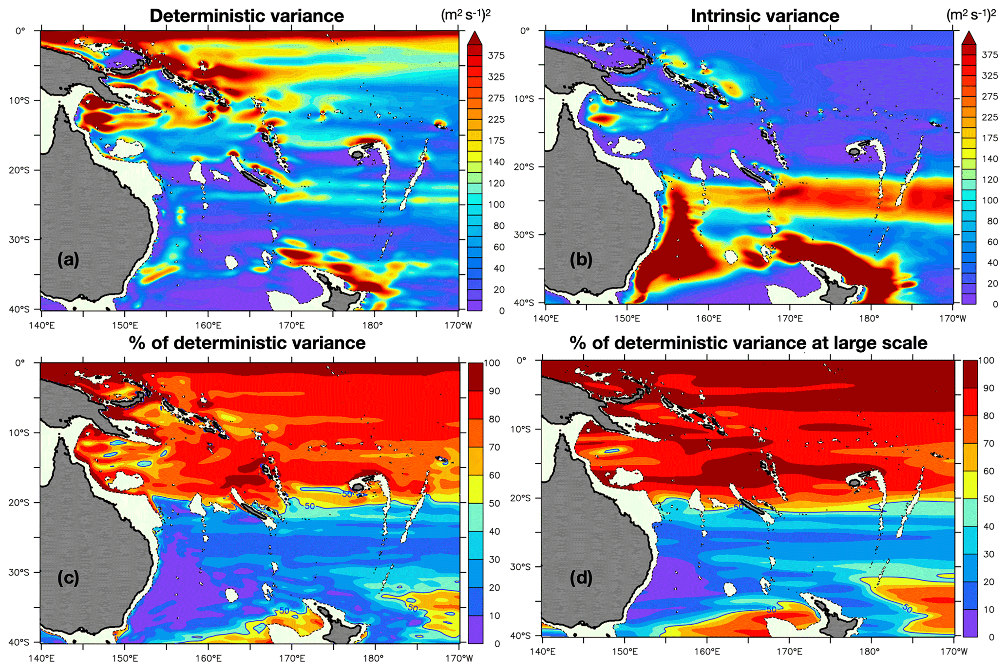
Figure 3 (a) Deterministic interannual variance: 1980–2015 variance of ensemble mean low-pass-filtered 0–1000 m zonal transport. (b) Intrinsic interannual variance: ensemble mean of the squared deviation of the low-pass-filtered 0–1000 m zonal transport in each member from the ensemble mean. (c) Ratio R_LF of the deterministic variance to the total variance, given as a percentage. (d) Same as (c), but for transports first spatially smoothed in each member.

The intrinsic interannual variability of zonal transports is particularly strong in three regions: in the EAC and East Auckland Current (EAUC) system regions and east and south of New Caledonia, all along the STCC path. Figure 3c reveals that in these regions, the intrinsic variability strongly dominates the deterministic variability at interannual timescales. This is particularly striking in the EAC extension region, where less than 5 % of the interannual variance is deterministic. Clearly, the regions exhibiting strong intrinsic variance coincide with the regions of high EKE, suggesting that mesoscale intrinsic high-frequency variability spontaneously cascades toward lower frequencies (Serazin et al., 2018).

The same computation is performed after a spatial smoothing of the transports over 10^∘ in longitude and 4^∘ in latitude to isolate the imprint of interannual intrinsic variability at larger scales (Fig. 3d). This anisotropic filtering takes into account the larger spatial scales in longitude of the zonal currents compared to the latitudinal scales. Although the relative contribution of intrinsic variability tends to be smaller for large-scale signals, the region where it dominates over the deterministic variance remains unchanged. The interannual intrinsic variability thus not only modulates small-scale transports at model grid points, but also has a strong imprint on large-scale, climate-relevant transports.

3.3 Variability of key currents transports

Interannual transport anomalies of key currents in the region are also computed in each member (see Sect. 2.1 and Table 1 for details and Fig. 2a for the locations of the sections), and their ensemble mean and spread are shown for monthly and interannual values in Fig. 4. The percentage of deterministic variance for each timescale is also given, together with the maximum correlation with the Nino3.4 index. No significant correlations are found with the SAM index. Clearly, the interannual variability of the transport entering the Coral Sea and the Solomon Sea as well as that of the NCJ is deterministic and correlated with ENSO (see also Sect. 4). Still, 5 %, 3 % and 7 %, respectively, of the interannual variance of these transports is chaotic (13 %, 9 % and 10 % for monthly means). On the other hand, the interannual variability of the transport of the SCJ, the Tasman Front and the EAC at various latitudes is largely chaotic and strongly impacted by ocean internal processes. At 32^∘ S, near the bifurcation latitude, only 14 % of the interannual transport variance is deterministic. In other words, inferring the interannual transport changes in these currents from a single simulation is very uncertain, as it will greatly depend on the initial conditions, and predicting them is very likely to be challenging. Surprisingly, the Tasman Front transport appears to be correlated with ENSO, with a 17-month lag. Also surprisingly, at the southern end of the region at 40^∘ S, the southern EAC extension transport is mostly deterministic, although it is known that a substantial fraction of this transport is driven by eddies (van Sebille et al., 2012; Oliver and Holbrook, 2014). Such deterministic interannual variability may arise from a substantial sensitivity of the mesoscale field itself to the interannual atmospheric forcing, which may then rectify the 0–1000 m transports in a rather deterministic way. Bull et al. (2017) have suggested that the mesoscale field characteristics and the mean EAC southern extension transport depend greatly on the local atmospheric variability, especially on the high-frequency local winds. Testing such a hypothesis is left for the future.

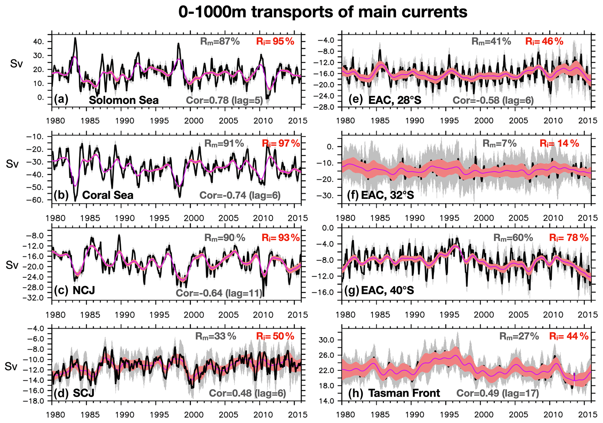
Figure 4 Time series of the 0–1000 m integrated transports across various sections (in Sv). In black: monthly values from the ensemble mean; in grey shades is the ensemble mean plus or minus the monthly ensemble spread. In red: interannual values from the ensemble mean, and the red shades represent the ensemble mean plus or minus the interannual ensemble spread. The percentage of the deterministic variance is given as R_m for the monthly values and R_i for the interannual values. The maximum correlation of the transport with the Nino3.4 index is also given, with the associated lag in months. (a) Meridional transport through the entrance of the Solomon Sea (positive is northward). (b) Zonal transport through the entrance of the Coral Sea (positive is eastward). (c) Westward transport of the NCJ. (d) Westward transport of the SCJ. (e) Meridional total transport of the EAC at 28^∘ S (see Sect. 2.3 for definition). R_m and R_i for the southward-only meridional transport are 44 % and 58 %, respectively. R_m and R_i for the northward recirculation branch are 21 % and 50 %, respectively. (f) Meridional total transport of the EAC at 32^∘ S. R_m and R_i for the southward-only meridional transport are 10 % and 29 %, respectively. R_m and R_i for the northward recirculation branch are 6 % and 22 %, respectively. (g) Meridional transport of the EAC at 40^∘ S. (h) Zonal transport of the Tasman Front. See text for details.

3.4 Variability of EKE

The same diagnoses are performed for the interannual variability of the EKE at 100 m and are shown in Fig. 5a–c. It is interesting to see that although some of the EKE modulation at interannual timescales is atmospherically forced (Fig. 5a), a significant amount of this interannual modulation is driven by ocean-only internal dynamics (Fig. 5b and c). This is especially striking between New Caledonia and New Zealand in the STCC–Tasman Front regions. These findings are not in agreement with Rieck et al. (2018), who concluded that the EKE low-frequency variability was mostly deterministic in the STCC region. The possible reasons for these different conclusions are discussed in Sect. 6. In the tropical band, the EKE interannual modulation is mostly atmospherically driven.

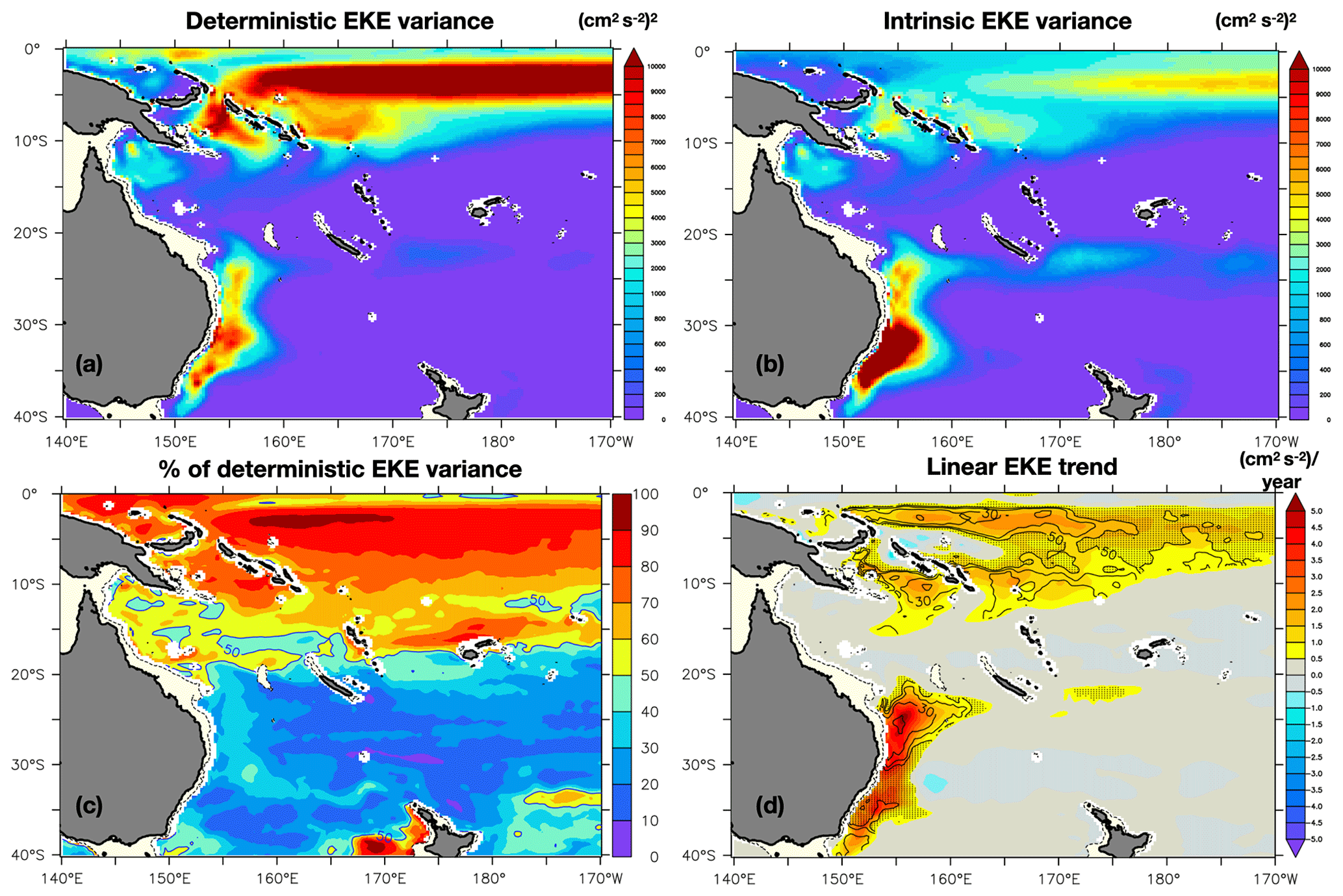
Figure 5 (a) Deterministic interannual variance of the EKE: 1980–2015 variance of ensemble mean low-pass-filtered 100 m EKE. (b) Intrinsic interannual variance: ensemble mean of the squared deviation of the low-pass-filtered 100 m EKE in each member from the ensemble mean. (c) Ratio R_LF of the deterministic EKE variance to the total EKE variance, given as a percentage. (d) 100 m EKE ensemble mean linear trend (in colors, ${\mathrm{cm}}^{\mathrm{2}}{\mathrm{s}}^{-\mathrm{2}}{\mathrm{yr}}^{-\mathrm{1}}$) and ratio of the spread between these linear trends and the deterministic trend (contours in percentage). The hatched areas show regions where the spread of these 1980–2015 EKE trends is higher than 50 % of the ensemble mean trend.

In addition to interannual variability, the lower-frequency evolution in EKE is also documented. Trends in both EAC and EAC extension transport have been reported in several studies (e.g., Cetenia-Heredia et al., 2014; Oke et al., 2019a), with a rapid strengthening of the eddy field since 2005 from 28^∘ S poleward. In the ensemble mean, as in all members, a positive linear trend in EKE is indeed found from about 20^∘ S poleward. But although the trend is largely deterministic around 25^∘ S, its actual value within individual members is mostly random south of 30^∘ S (Fig. 5c).

3.5 Variability of the EAC separation latitude and of the SEC bifurcation

Finally, diagnoses are also done for more integrated quantities. The latitude of the EAC separation latitude is computed in each member following Cetina-Heredia et al. (2014) and Oke et al. (2019a). The sea surface height (SSH) isoline at 28^∘ S (where the EAC stream is well defined) associated with the maximum southward geostrophic current is identified and followed southward until it veers eastward (i.e., when the SSH isoline longitude starts to increase). The corresponding latitude is identified as the separation latitude (Fig. 6a), and its ensemble mean and spread are shown in Fig. 6b for monthly and interannual time series.

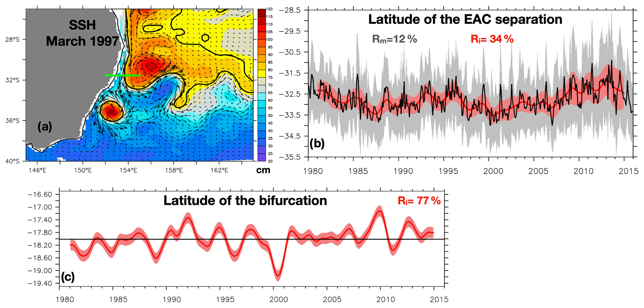
Figure 6 (a) Sea surface height (SSH) snapshot from one member on 15 March 1997 (colors), with the isoline associated with the maximum southward geostrophic current at 28^∘ S (thick black line), and geostrophic surface currents (vectors). The latitude of the EAC separation in that snapshot, at which the isoline veers eastward, is indicated by the thick green line. (b) Time series of the latitude of EAC separation. In black: monthly values from the ensemble mean; in grey shades is the ensemble mean plus or minus the monthly ensemble spread. In red: interannual values from the ensemble mean, and the red shades represent the ensemble mean plus or minus the interannual ensemble spread. The percentage of the deterministic variance is given as R_m for the monthly values and R_i for the interannual values. (c) Time series of the latitude of western boundary current bifurcation. In red: interannual values from the ensemble mean, and the red shades represent the ensemble mean plus or minus the interannual ensemble spread. In black: the 1980–2015 average latitude of the bifurcation. The percentage of the deterministic variance is given as R_i for the interannual values.

The latitude of the westward SEC bifurcation at the coast of Australia (i.e., the latitude separating waters that further flow into the equatorial system from those that feed the EAC) is an important quantity that is climatically relevant for the distribution of water masses equatorward and poleward. This latitude, defined as the latitude along the coast of Australia at which the 0–1000 m meridional transport changes from equatorward to poleward, is also computed from the interannual meridional currents in each member and is shown in Fig. 6c. Its mean is 18^∘ S, similar to what was estimated by Kessler and Cravatte (2013a) from linear, wind-driven “island rule” streamfunction estimations (Godfrey, 1989) and observations. Interannually, the ensemble mean moves from 19.1 to 17.1^∘ S, and these displacements are positively correlated with the Nino3 index (0.52) with a 2-month lag. The interannual variability of the bifurcation latitude is mostly deterministic (R=77 %).

The latitude where the EAC separates from the coast can vary abruptly at intraseasonal timescales, as eddy detachments lead to northward displacements of the separation point. This latitude strongly varies from one member to the other, as eddies development and detachments are not synchronous. The eddy-shedding events are clearly intrinsic, although their timing has been shown to be partly controlled by atmospheric forcing modulation (Bull et al., 2017). Interestingly, the interannual variability of the EAC separation latitude is also strongly dominated by intrinsic variability, since the deterministic variance only represents 34 % of the variance. No significant correlation with ENSO is found, whereas Cetina-Heredia et al. (2014) suggested that the relaxation of an ENSO event induces a shift in the EAC separation latitude. It confirms that the definition of a bifurcation latitude, and of a well-defined continuous eastward flow emanating from the coast, is not an adequate description of the eddying circulation (Oke et al., 2019b).

4 Drivers of deterministic variability

4.1 0–1000 interannual transport

The extent to which the interannual variability of the transports in the southwestern Pacific is driven by ENSO or other climate-related indices (contained in the prescribed atmospheric forcing) is now explored. Firstly, it is explored within one member picked randomly. Figure 7a shows the maximum lagged correlation between the Nino3.4 index and the 0–1000 m transports in member 39, with the corresponding lag in months (Fig. 7c). Positive correlations mean that the transport increases in relation to Nino3.4, and negative lags mean that Nino3.4 leads the transport variations. Significant correlations are found north of 20^∘ S, with positive anomalies in the equatorial band and south of 10^∘ S a few months after Nino3.4. This corresponds to eastward anomalies at the Equator and westward anomalies in the transport entering the Coral Sea. Positive (northward) anomalies in the LLWBC through the Solomon Sea are also found, in agreement with previous findings. A few months after an El Niño event, a dipole of wind stress curl anomalies is found over the South Pacific from 5 to 30^∘ S and 150^∘ E to 140^∘ W. These wind stress curl anomalies induce an increase in the westward SEC transport entering the Coral Sea (Kessler and Cravatte, 2013b) and an increase in the NGCU into the Solomon Sea (Melet et al., 2013; Davis et al., 2012; Kessler et al., 2019), mainly in the top 250 m. The lag increases with latitude, as expected from the poleward decrease in Rossby wave westward phase speed, as these waves are the means by which the curl modifications are transmitted across the ocean toward the western Pacific. It is also found that the EAC poleward velocity increases 6 to 15 months after an El Niño north of 30^∘ S. Further south, the map is noisy, and no significant correlations are found at any lag.

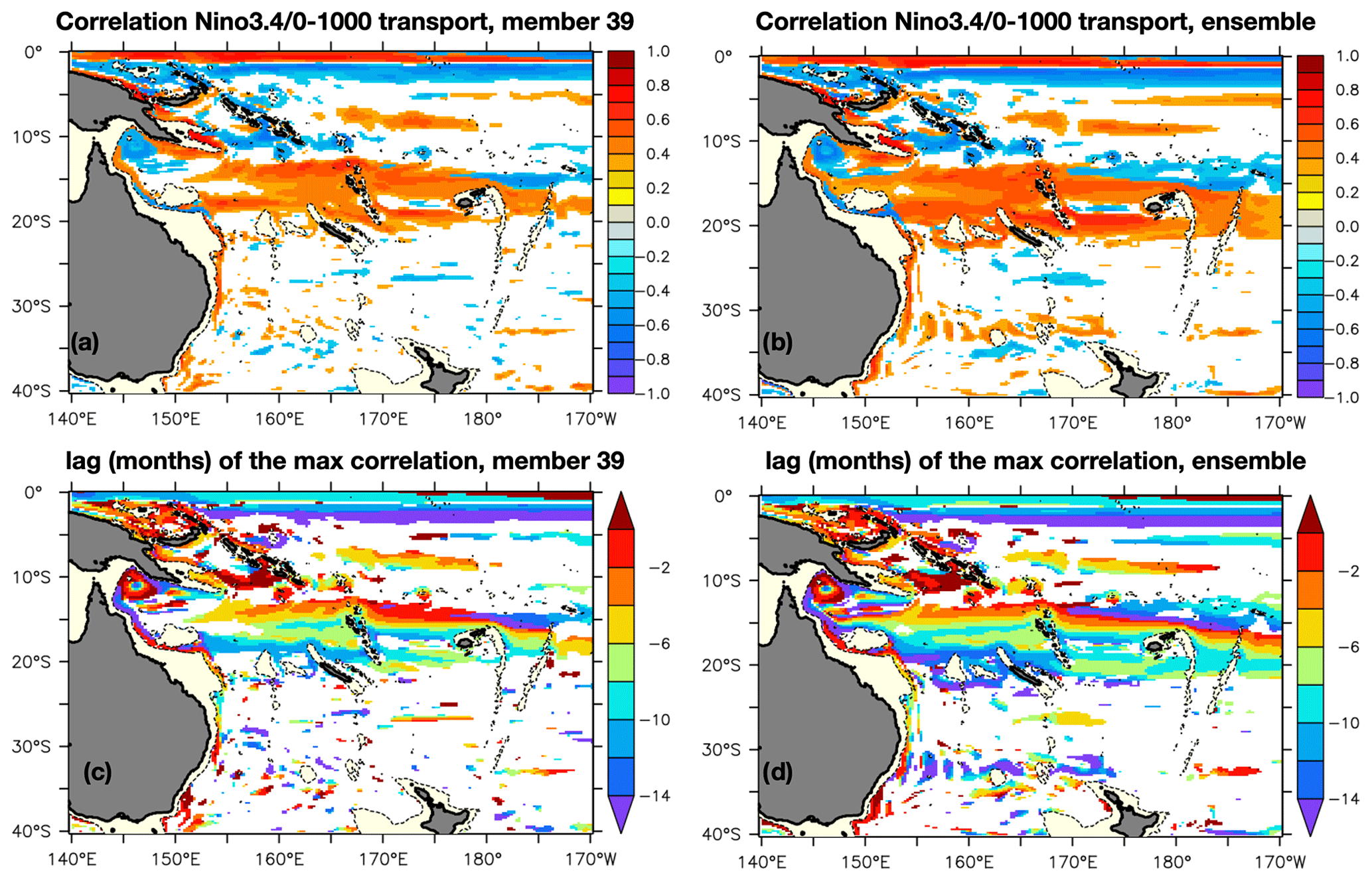
Figure 7 Maximum lagged correlation (a, b) and corresponding lag in months (taken between −15 and 5 months) (c, d) between the Nino3.4 index and the 0–1000 m interannual transport variations for (a, c) member 39 of the ensemble and (b, d) the ensemble mean. A negative lag means that Nino3.4 leads the transports variations. Only significant correlations are plotted.

The same analysis is now done with the ensemble mean. Interestingly, in addition to the significant correlations found in member 39, additional patterns emerge. Some of the transports south of New Caledonia also exhibit a correlation with ENSO. The SCJ (around 27^∘ S, 170^∘ E) decreases a few months after an El Niño, and the latitude of the Tasman Front maximum transport also emerges as significantly correlated with ENSO, shifting northward 15 months after an El Niño. This reveals that chaotic oceanic variability can mask the ENSO imprint on interannual transport variability south of 20^∘ S and that an ensemble mean allows us to better identify this ENSO imprint. Whether an ensemble mean computed from more than 50 members would yield more regions with significant correlations is not known, and the number of members needed to converge would be worth investigating.

Similar correlations were computed with the PDO index and the SAM index (not shown). The EAC separation latitude and the Tasman Front latitudinal extension appear to move southward 10 to 15 months after a positive SAM. During a positive PDO phase, the patterns of transport changes are very similar to the ENSO ones, with a stronger signal in the Tasman Front region where the transport increases, while the EAC southward extension decreases. These anticorrelated decadal variations in both currents are consistent with previous findings (Hill et al., 2011; Sasaki et al., 2008). All these correlations are somewhat clearer in the ensemble mean than in individual members.

4.2 EKE

Figure 8a shows the maximum lagged correlation between the Nino3.4 index and the 100 m EKE from the ensemble mean, with the corresponding lag in months. Two regions of significant correlation emerge: the tropical band, including the Solomon Sea, and the Tasman Front region. A few months after an El Niño, EKE decreases in the tropics, consistent with findings from Tchilibou et al. (2020); 15 months after an El Niño, EKE conversely increases in the Tasman Front area when the Tasman Front is stronger and shifted northward.

Figure 8 Maximum lagged correlation (a) and corresponding lag in months (taken between −18 and 0 months) (c) between the Nino3.4 index and the 100 m EKE interannual variations for the ensemble. Only significant correlations are plotted. A negative lag means that Nino3.4 leads the EKE variations. (b, d) Same as (a, c) for the PDO index. In all panels, the hatched areas show regions where the same maximum lagged correlation for 100 m EKE interannual variations in one member picked randomly (member 39) is not significant.

The EKE is also modulated at decadal timescales in connection with the PDO in the STCC region, as suggested previously by Rieck et al. (2018) and Travis and Qiu (2017) (Fig. 8b). During positive phases of the PDO, the EKE decreases in the whole STCC band, in addition to the equatorial band. The processes explaining this decadal deterministic modulation have been investigated in Rieck et al. (2018) and Travis and Qiu (2017). EKE is modulated through a mix of processes including changes in large-scale zonal current strength, associated vertical shear and stratification. These changes, forced by decadal wind changes in the subtropical gyre, work simultaneously to modify the baroclinic instability intensity and the EKE levels. As shown in Fig. 5c, this deterministic forcing, however, only represents 10 % to 30 % of the EKE variability at interannual timescales. It is worth noting that these correlations do not clearly emerge in individual members (see dots in Fig. 8).

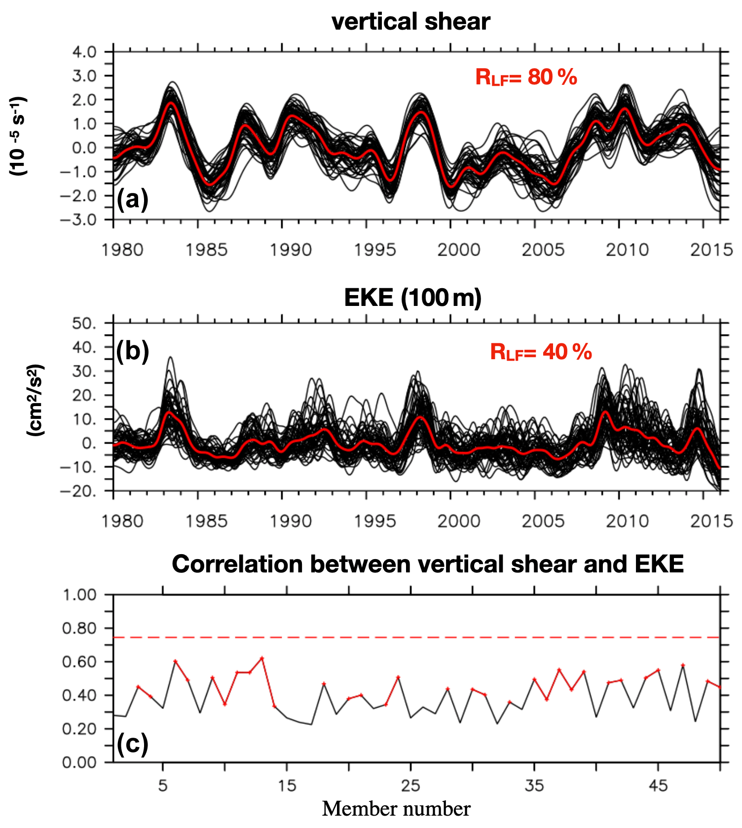
Figure 9 Time series of the vertical shear (10⁻⁵ s⁻¹) (a) and EKE at 100 m (cm² s⁻²) (b) interannual anomalies averaged in the STCC region (28–22^∘ S, 160–180^∘ E). In black: values from the 50 members; in red: values from the ensemble mean. (c) Correlation between the vertical shear and the EKE interannual anomalies for all the members (in black), with the x axis corresponding to the 50 members and the ensemble mean (in dashed red). The correlations significantly different from zero at the 95 % confidence level are overlaid in red. The ratio R_LF of the deterministic variance to the total variance as a percentage is given for the shear and the EKE.

We further examine the correlation between the vertical shear (defined as the difference between the zonal current at 600 m and at 200 m) (see Travis and Qiu, 2017) and the EKE levels in the STCC region (160^∘ E–180^∘, 22–28^∘ S) (Fig. 9). In the ensemble mean, a significant correlation (0.75) is found between the shear and the EKE (Fig. 9c, red dashed line), as also found in altimetric data and a reanalysis in Travis and Qiu (2017) and an OGCM simulation in Rieck et al. (2018). In each individual member, however, there is not always a significant correlation between vertical shear and EKE amplitude. The vertical shear appears to be driven at least partly by the atmospheric forcing, as the members do not exhibit a substantial dispersion (Fig. 9a), and 80 % of the variance is deterministic. In contrast, the EKE interannual modulation is dominantly intrinsic (Fig. 9b), as only 40 % of the variance is deterministic. These results highlight the complexity of EKE generation and the interplay of different forcing processes, whose relative importance varies. The vertical shear, the stratification and the propagations of eddies from remote regions may all influence the EKE levels. Travis and Qiu (2017) showed that these processes vary in time and can alternately work to attenuate or reinforce each other. Here, we suggest in addition that they vary differently in the members and can alternately attenuate or reinforce each other in the different members.

5 Spatiotemporal structure of the chaotic oceanic variability

What are the processes at work producing interannual intrinsic variability? How do mesoscale eddies impact the transport interannual variability? Is chaotic oceanic variability spatially coherent at large scale? To provide some possible answers, we now look at individual members and analyze the chaotic variability in these members with EOF (empirical orthogonal function) analyses for both monthly and interannual time series.

Two regions of large oceanic chaotic variance are examined in more detail: (a) the EAC extension region from 30 to 40^∘ S and (b) the STCC area where both transport and EKE modulation are dominantly chaotic. In each member, the deviations from the ensemble mean of zonal and meridional transports at monthly and interannual timescales are computed. A multivariable EOF analysis is first performed on both components of the transport for individual members (Dawson, 2016). Additionally, the 50 members are combined to produce a 50× (1980–2015) time series on which a multivariable EOF analysis is performed for zonal and meridional transports. This allows isolating the spatial patterns of chaotic variability common to all members, while allowing them to have different timings revealed by their PCs (principal components). The first two EOFs emerging from the individual EOF analysis are similar to those emerging in the 50-member combined EOF analysis, giving confidence to the robustness of the signals.

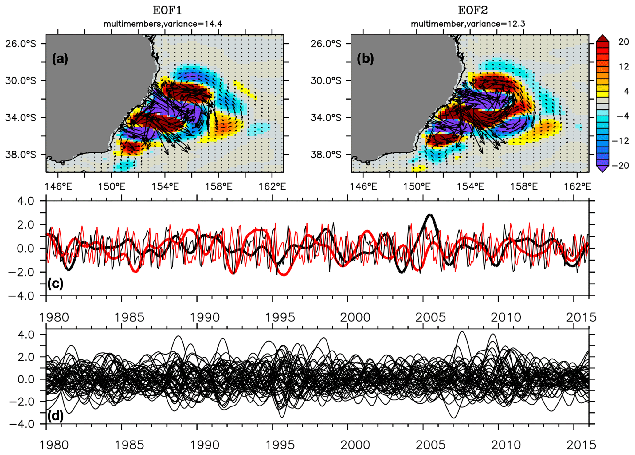
Figure 10 First (a) and second (b) spatial EOFs in the EAC region (25–40^∘ S, 145–163^∘ E) for the deviations of the 50 members from the ensemble mean of zonal and meridional transports considered as a single time series. (c) PCs of the first (black) and second (red) mode from monthly chaotic transports shown by thin lines and interannual chaotic transports shown by thick lines for member 1. (d) The PCs of the first mode from interannual chaotic transports of the 50 members.

In the EAC region (Fig. 10), the monthly EOFs reveal the presence of mesoscale eddies with periods of 100–180 d, as shown by previous studies (e.g., Oke et al., 2019a). Figure 10c shows the associated monthly and interannual PCs extracted for member 1, and Fig. 10d shows the other PCs for the 50 members. The eddy amplitude envelope is modulated in time. In all members, the characteristics of the eddies are similar (periods, amplitude), as expected since they share the same model dynamics. However, the phasing of the eddies, and of the lower-frequency interannual chaotic fluctuations, is random and differs among the members. Further investigating the nonlinear interactions leading to the transport interannual variability, probably arising from eddy low-frequency rectification, would be interesting but is beyond the scope of this study.

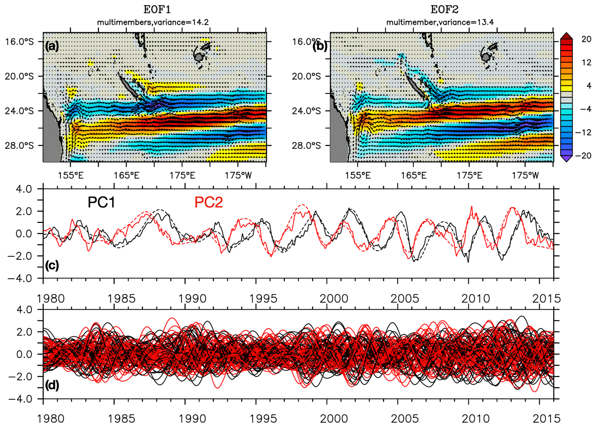
Figure 11 First (a) and second (b) spatial EOFs in the STCC region (15–30^∘ S, 150^∘ E–170^∘ W) for the deviations of the 50 members from the ensemble mean of zonal and meridional transports considered as a single time series. (c) PCs of the first (black) and second (red) mode from monthly chaotic transports shown by thin lines and interannual chaotic transports shown by dashed lines for member 1. (d) The PCs of the first (black) and second (red) modes from interannual chaotic transports of the 50 chaotic members.

In the STCC region, the spatial structure of the chaotic variability is quite different (Fig. 11a and b). In terms of zonal transport, it consists of zonally elongated structures that alternate meridionally, are slanted in a southwest–northeast direction and slowly propagate southward, as can be seen when comparing the first two EOFs and PCs. Such striation-like structures have already been noticed in the western half of subtropical basins with low-passed altimetric observations (Maximenko et al., 2005) and on global maps of sea level intrinsic variability (Serazin et al., 2015, their Fig. 4). These fluctuating striations might be generated by an incomplete anisotropic inverse cascade from small-scale intraseasonal structures like eddies towards low-frequency zonally elongated structures (see Sect. 6 of Serazin et al., 2018, for a complete discussion). Because some parameters might prevent the inverse cascade from reaching the basin scale – including the presence of a meridional mean flow (Chen and Flierl, 2015), the intensity of bottom friction (Berloff et al., 2009; 2011) and the presence of meridional boundaries (Lacasce, 2002) – these striations cannot develop into persistent zonal jets as in the atmosphere but rather behave as weak latent jets that show up only on filtered signals such as the EOF decomposition performed here.

Interestingly, monthly and interannual EOFs and PCs are similar (Fig. 11c), revealing that large-scale intrinsic variability in this area is dominated by a low-frequency (3–4-year timescale) signal. These anomalies have a random, time-evolving phase difference among the members, confirming that they arise from ocean-driven intrinsic processes, potentially through nonlinear scale interactions (i.e., an inverse cascade) as discussed above.

6 Discussion and conclusion

In this study, the origin and features of interannual variability of the transports and EKE in the southwestern Pacific have been investigated using a probabilistic modeling strategy. A large ensemble of 50 simulations performed with the same OGCM at eddy-permitting resolution, perturbed initially but driven by the same realistic atmospheric forcing over 1980–2015, has been analyzed to disentangle the atmospherically forced deterministic ocean variability and the internal chaotic ocean variability. This approach was previously used to show that chaotic oceanic processes can have more impact than atmospheric variability on the low-frequency variability and trends of regional transport, sea level and oceanic heat content, particularly at mid-latitudes (Leroux et al., 2018; Llovel et al., 2018; Serazin et al., 2017).

Our results show that in the southwestern Pacific, the interannual variability of the transports is strongly dominated by chaotic oceanic variability south of 20^∘ S. In the tropics, while the interannual variability of transports and EKE modulation is largely deterministic and explained by ENSO, oceanic chaotic processes may still explain 10 % to 20 % of the interannual variance at large scale and can reach 40 % to 60 % locally in areas of complex topography such as the Gulf of Papua, inside the Solomon Sea and east of the Solomon Islands. Regions of strong chaotic variance generally coincide with regions of high mesoscale activity; the interannual chaotic ocean variability is greater when the EKE is larger, suggesting that a spontaneous inverse cascade is at work from the mesoscale toward lower frequencies and larger scales, in agreement with Serazin et al. (2018). The small random perturbations introduced in the initial states progressively grow in amplitude due to oceanic nonlinearities, generating the emergence of out-of-phase mesoscale perturbations among the members. As the ensemble spread tends to saturate in amplitude, the spatial and temporal scales of the intrinsic variability continue to grow through nonlinear inverse cascades of energy (Arbic et al., 2014; Sérazin et al., 2018).

The spatial and temporal features of the oceanic chaotic variability are complex and vary from region to region. Interestingly, as the simulations share the same dynamics, they produce chaotic structures with similar spatial characteristics but with different phasing. In the STCC, the low-frequency imprint of these structures is zonally elongated, and its spatial organization is likely the result of an incomplete anisotropic inverse cascade due to nonlinear scale interactions (e.g., Sérazin et al., 2018). In other regions, they are eddy-shaped. The physical processes governing this chaotic variability remain to be fully understood.

Our results on the origin of the EKE variability (dominantly intrinsic) are in contrast with the findings of Rieck et al. (2018), who concluded that the EKE decadal variability in the STCC region was, uniquely among the subtropical gyres, mostly deterministic and driven by wind-forced decadal changes. In agreement with the Travis and Qiu (2017) analyses of observations, they explained these decadal EKE modulation through decadal changes in vertical shear driven by wind stress curl changes in the South Pacific, while still recognizing that other processes such as changes in stratification or remotely forced density anomalies also contribute to modulating the EKE low-frequency changes. It is worth mentioning that our analyses are not directly comparable: firstly, the regions considered in these two studies differ from our region of focus here and are much larger, extending eastward to the central part of the basin. Yet, Rieck et al. (2018) found a mostly deterministic EKE variance also in the 22–28^∘ S to 160^∘ E–180^∘ region considered here, as can be seen in their Fig. 2. Secondly, Rieck et al. (2018) studied the EKE decadal variability, whereas we focus on interannual timescales. As we go toward larger spatial and temporal scales, it is probable that the intrinsic contribution to the total variance would diminish. It is also worth noting that we adopted a different modeling strategy here. Rieck et al. (2018) used a long climatological run to study the sole imprint of intrinsic interannual variability. Here, we use 50 members with fully varying atmospheric forcing, which gives access to both intrinsic and atmospherically driven interannual oceanic fluctuations. Fully understanding the reasons behind our different conclusions on the EKE variability nature would require more analyses, which are beyond the scope of this paper.

In agreement with Rieck et al. (2018) and Travis and Qiu (2017), we found a link between the low-frequency variations of vertical shear in the STCC region and EKE modulation in the ensemble mean. However, in each member, we found that other processes (probably such as stratification changes, and propagations of eddies from remote regions) all contribute to modulating the EKE levels, with the contribution of the vertical shear having a different relative importance in the different members. These results highlight the complexity of EKE generation and the interplay of different forcing processes; they also emphasize the importance of simultaneously taking into account the chaotic ocean behavior and the imprint of the atmospheric variability in an ensemble approach. It is also worth noting that our results do not question the existence of deterministic, forced interannual variability of EKE in the area; our results mostly emphasize the fact that the chaotic ocean interannual variability may overwhelm this deterministic variability over large regions.

The fraction of interannual variability explained by chaotic oceanic processes depends on the spatial scale considered. At model grid points, this fraction is greater than for spatially integrated variables or large-scale transports across sections. Yet, our results show that for some key currents, section-integrated transport variability is dominantly chaotic. Moreover, our study reveals that chaotic variability may result in large-scale, spatially coherent signals at interannual timescales. The EAC separation latitude variability (defined where eddies detach from the EAC) at interannual timescales is also largely chaotic.

These results have important implications for the understanding and forecasting of the transports in the region and for observational strategies. Firstly, they show that the impact of climate modes of variability such as ENSO and PDO on the interannual variability of transports and EKE may be hidden by oceanic internal variability and that an ensemble of simulations is needed to bring out this signature. This clearly hampers our capacity to attribute the forced origin of the interannual variability of transports from a single simulation.

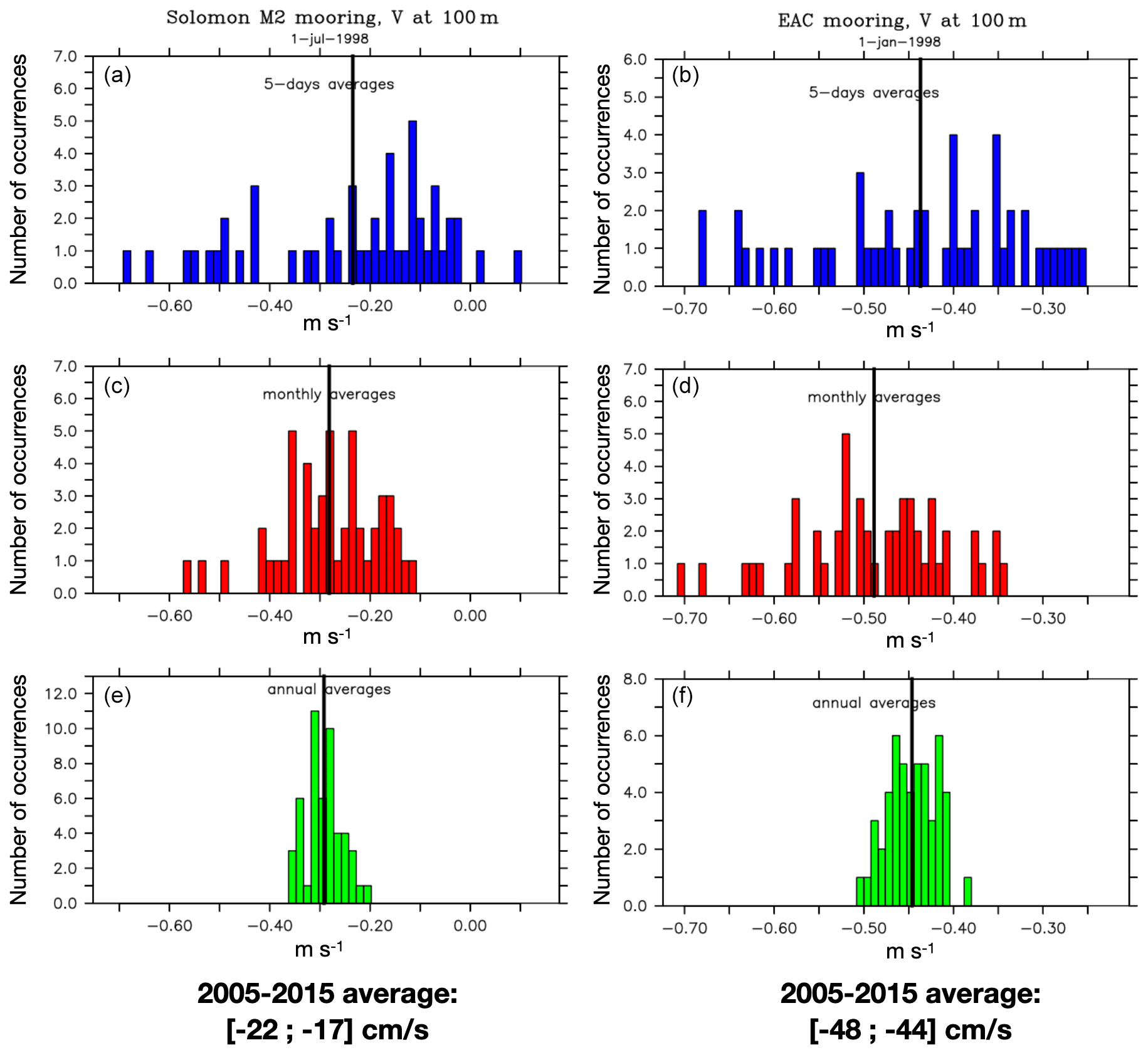
Figure 12 Histograms of velocity among the 50 members for the meridional velocity at 100 m from 5 d average values in blue (a, b), monthly averages in red (c, d) and annual averages in green (e, f) at two locations around a particular date (1 July 1998 inside the Solomon Strait at 154.2^∘ E, 5.36^∘ S – a, c, e; 1 January 1998 in the EAC at 154^∘ E, 27.06^∘ S – b, d, f). The ensemble means are also plotted as black lines.

Importantly, these results highlight the fact that the interpretation of in situ or satellite observations in areas of high intrinsic variance should be done with caution. While the low-frequency signal amplitude does not strongly vary between members, intrinsic variability gives their phase a stochastic flavor and tends to decorrelate the oceanic variability from the atmospheric variability. Figure 12 illustrates how chaotic ocean variability can imprint synthetic (i.e., model-simulated) mooring measurements at various timescales. Histograms of the meridional velocity at 100 m for the 50 members at existing moorings locations in the EAC (at 27^∘ S) and in the Solomon Sea Strait (Alberty et al., 2019; Sloyan et al., 2016) are shown on a given date for 5 d averages, monthly averages, yearly averages and 2005–2015 averages. It is shown that even for an instrument deployed in a mostly deterministic current such as the New Ireland Coastal Undercurrent (NICU) in the Solomon Strait, the dispersion of values can be large. If one considers the fact that an in situ observation samples one ocean state randomly picked from an ensemble of possibilities, the larger the intrinsic variability, the less representative an observation is, and the less its interannual variability can be attributed to the atmosphere; thus, the less it can be predicted and understood deterministically. This also suggests that assimilation of these data in numerical simulations should consider this additional source of uncertainty. The repercussions of errors in gridded products based on individual profiles, such as in Argo temperature and salinity gridded products or satellite-track gridded products, should be usefully evaluated (see also Penduff et al., 2018, their Fig. 2 and the associated discussion about the representativeness of temperature measurements). Such studies are currently underway.

It should be kept in mind that we used an eddy-permitting ($\mathrm{1}/\mathrm{4}$^∘) resolution that sits at the limit of presently affordable long-term global ocean large ensembles, but at which only some of the mesoscale activity is simulated. It is probable that at higher resolution, with the increased mesoscale activity, inverse cascades of energy toward large scales and low frequencies are stronger: this has been shown in terms of sea level by Serazin et al. (2015), who suggested a direct feeding of low-frequency chaotic variability by mesoscale activity both within and away from eddy-active regions. Gregorio et al. (2015), however, have suggested that the forced variability of the Atlantic Meridional Overturning Circulation (AMOC) is also likely to increase when switching from $\mathrm{1}/\mathrm{4}$^∘ to $\mathrm{1}/\mathrm{12}$^∘ resolution; whether this also holds for the variables investigated here needs to be verified, but these authors did not report a substantial sensitivity of forced-to-total variability ratios (denoted as R_LF here) to this resolution increase. More generally, it would be interesting to assess whether the OCCIPUT ensemble gives a robust estimate of the ocean chaotic variability; comparisons with other ensemble simulations (such as that performed at $\mathrm{1}/\mathrm{10}$^∘ by Nonaka et al., 2020) would be of use for such an assessment.

We also used forced and not coupled oceanic simulations, which is an indispensable step to isolate the chaotic ocean-only contributions. The importance of air–sea interactions at the mesoscale, however, is known to be significant. The wind stress variability is impacted by the ocean current feedback, which could dampen the EKE eddy-scale variability in return (e.g., Renault et al., 2017, 2019). Intrinsic variability is also likely to impact the air–sea heat flux variability through sea surface temperature fluctuations and affect the atmospheric variability in return. These possible effects should be investigated in the future as the observed variability reflects the fully coupled climate system.