Multidecadal polynya formation in a conceptual (box) model

Maud Rise polynyas (MRPs) form due to deep convection, which is caused by static instabilities of the water column. Recent studies with the Community Earth System Model (CESM) have indicated that a multidecadal varying heat accumulation in the subsurface layer occurs prior to MRP formation due to the heat transport over the Weddell Gyre. In this study, a conceptual MRP box model, forced with CESM data, is used to investigate the role of this subsurface heat accumulation in MRP formation. Cases excluding and including multidecadal varying subsurface heat and salt fluxes are considered, and multiple polynya events are only simulated in the cases where subsurface fluxes are included. The dominant frequency for MRP events in these results, approximately the frequency of the subsurface heat and salt accumulation, is still visible in cases where white noise is added to the freshwater flux. This indicates the importance and dominance of the subsurface heat accumulation in MRP formation.

1 Introduction

The Weddell Sea is a region where open-ocean polynyas occasionally form. A distinction is made between the larger Weddell Sea polynyas (WSPs) and the smaller Maud Rise polynyas (MRPs). Formation of the MRPs is clearly related to bathymetry, i.e., Maud Rise, an underwater seamount, whereas this clear relation is absent for WSPs. The first polynyas in the Weddell Sea were observed in the 1970s around 65^∘ S and 0^∘ E (Martinson et al., 1981) with in situ observations (Gordon, 1978) and the first available satellite images (Carsey, 1980). In 1974, 1975, and 1976, polynyas with an areal extent of approximately 2.5 × 10⁵ km² were present throughout the winter (Gordon et al., 2007) and can be classified as WSPs. An MRP appeared in 2016 and 2017 (Jena et al., 2019). The 2017 MRP had an approximate area of 0.5 × 10⁵ km² and persisted from September to October (Campbell et al., 2019; Cheon and Gordon, 2019). Observations also suggest a short-lived and small-scale MRP in 1994 (Holland, 2001; Lindsay et al., 2004). In this paper, we will focus specifically on MRPs.

Many studies have looked into the processes responsible for MRP formation. A key theory is that MRPs are formed by deep convection caused by static instability due to surface salt anomalies in a preconditioned water column (Martinson et al., 1981). Such salt anomalies can be caused by brine rejection (Martinson et al., 1981) but also by freshwater flux anomalies due to variations in the Southern Annular Mode (Gordon et al., 2007; Cheon and Gordon, 2019). Another line of work focuses on dynamical forcing by the wind (Parkinson, 1983; Francis et al., 2019; Jena et al., 2019; Campbell et al., 2019) as a cause of MRP formation. A divergent wind stress can open up the sea-ice pack and induce upwelling (by Ekman dynamics) which either causes an MRP directly or induces deep convection. Finally, dynamical forcing through ocean eddy shedding at the flanks of Maud Rise (Holland, 2001) and Taylor caps above Maud Rise (Alverson and Owens, 1996; Kurtakoti et al., 2018) can change the background stratification and, hence, precondition the water column. These processes also cause a general halo of relatively low sea-ice concentrations over Maud Rise (Lindsay et al., 2004).

Climate models provide the opportunity to study deep convection and, consequently, MRP formation. From several climate models, it is known that deep convection in the Southern Ocean varies on multidecadal to multicentennial timescales (Martin et al., 2013; Zanowski et al., 2015; Latif et al., 2017; Weijer et al., 2017). Several climate models show subsurface heat accumulation prior to deep convection, e.g., in the Kiel Climate Model (KCM) (Martin et al., 2013), the Community Earth System Model (CESM) (van Westen and Dijkstra, 2020a), and the Geophysical Fluid Dynamics Laboratory Climate Model (GFDL CM2-0) (Dufour et al., 2017). Through buoyancy gain in the subsurface layer, deep convection is induced, which results in MRP formation (Martin et al., 2013; Latif et al., 2017; Reintges et al., 2017). In the KCM, for example, a stronger stratification results in a longer period for deep convection, because more buoyancy gain is necessary to overcome the more stable stratification (Latif et al., 2017; Reintges et al., 2017). Another important feature is model resolution, as shown by Weijer et al. (2017): MRPs were found in a high-resolution (0.1^∘) version of the CESM, whereas no MRPs were simulated in the low-resolution (1^∘) version of the same model. Dufour et al. (2017) used the GFDL CM2-0 model with a nominal ocean grid spacing of 0.25 and 0.1^∘ and showed that the occurrence of deep convection itself is not sufficient to create MRPs. If the subsurface heat reservoir cannot supply enough heat to melt all of the sea ice, an MRP will not form.

A recent model study by van Westen and Dijkstra (2020a) showed a multidecadal occurrence of MRPs and suggested that the timescale of MRP formation is affected by intrinsic ocean variability through subsurface preconditioning. They relate the subsurface heat accumulation near Maud Rise to the Southern Ocean Mode (SOM), a multidecadal mode of intrinsic variability in the Southern Ocean caused by eddy-mean flow interactions (Le Bars et al., 2016; Jüling et al., 2018), which is present in high-resolution (ocean) models (van Westen and Dijkstra, 2017). The study by van Westen and Dijkstra (2020a) showed that heat content anomalies propagate from the SOM region (50–35^∘ S × 50–0^∘ W) via the Antarctic Circumpolar Current (ACC) to 30^∘ E and from the Weddell Gyre to the Maud Rise area, where they cause heat accumulation in the subsurface layer. The CESM model results are further analyzed in van Westen and Dijkstra (2020b), where the importance of this subsurface heat accumulation on the MRP formation is shown.

To better understand the results of the high-resolution CESM simulations (van Westen and Dijkstra, 2020a, b) and to connect to earlier theories of MRP formation, we use an extension of the Martinson et al. (1981) box model here. This extended version of the Martinson model is described in Sect. 2. Results for five different cases are considered (Sect. 3), in order to address the importance of subsurface forcing (i.e., heat and salt accumulation) relative to surface forcing (e.g., brine rejection and wind forcing) in MRP formation, as are the processes determining the long-term variability of MRPs. In Sect. 4, a summary and a discussion of the results are given.

2 Model description and cases considered

The model used is based on the box model proposed in Martinson et al. (1981). Note that this box model was originally developed for Weddell Sea polynyas (WSP). Martinson et al. (1981) proposed that convection was initiated by surface salinity anomalies, similar to the surface-initiated convection processes suggested during MRP formation (Kurtakoti et al., 2018; Campbell et al., 2019; Cheon and Gordon, 2019; Kaufman et al., 2020). Stratified Taylor columns contribute to the preconditioning of the Maud Rise region by lowering the stratification over Maud Rise compared with the surroundings (Alverson and Owens, 1996; de Steur et al., 2007; van Westen and Dijkstra, 2020a). Nonetheless, a distinct surface and subsurface layer is present over Maud Rise, which can be simplified by two boxes, as is done in Martinson et al. (1981). The original box model is applicable to the Maud Rise with some adjustments. This new model is described in Sect. 2.1, the CESM simulation used in this study is shortly described in Sect. 2.2, and the different configurations and cases for the box model are presented in Sect. 2.3.

2.1 Model description

The MRP box model consists of two vertically stacked boxes with a constant depth, and the ocean properties (e.g., temperature and salinity) are uniform within each box. The model simulates the development of temperature (T), salinity (S), and sea-ice thickness (δ) in each box under surface and subsurface forcing. The depth of the entire water column is H, the surface layer has a depth of h₁, and the subsurface layer has a depth of h₂.

The model has four different flow regimes, referred to as regimes I–IV in the following, which are differentiated using sea-ice cover (sea-ice-free versus sea-ice-covered areas) and static stability (two-layered versus mixed). Whenever stable or unstable is mentioned below, we refer to static stability of the water column, so no dynamical instabilities are considered. There are the sea-ice-free regimes (regimes I and II) and sea-ice-covered regimes (regimes III and IV). Regimes II and IV are stably stratified (ρ₁<ρ₂), and regimes I and III are mixed with one uniform density over the entire depth (Fig. 1). The subscripts 1 and 2 correspond to the surface and subsurface layer, respectively.

Over time, the model state may transit through these four regimes under the influence of (seasonal) forcing. The four different regime transitions are indicated by the arrows in Fig. 1:

• a.

  from sea-ice-covered regimes to sea-ice-free regimes due to the complete melt of the sea ice (δ=0) (regime IV → II or regime III → I);

• b.

  from sea-ice-free regimes to sea-ice-covered regimes, because the surface layer reaches freezing and sea ice starts to form (T₁=T_f) (regime II → IV and regime I → III);

• c.

  from stable, two-layered regimes to unstable, mixed regimes, because the density of the surface layer is equal to or larger than that of the subsurface layer (ρ₁≥ρ₂) (regime II → I and regime IV → III). The water column becomes unstable and mixes through overturning. Temperature and salinity are uniform over the entire layer and are indicated by T and S instead of T_n and S_n;

• d.

  from unstable, mixed regimes to stable, two-layered regimes, because of stabilization of the water column due to a decreasing density of the mixed layer (regime I → II and regime III → IV).

The precise conditions for the regime transitions are shown in Appendix A. It should be noted that for the model to switch between regimes I (mixed, sea-ice-free regime) and III (mixed, sea-ice-covered regime), the entire water column should reach freezing temperature, which is physically not realistic. Therefore, this transition does not exist in the model (regime I  regime III).

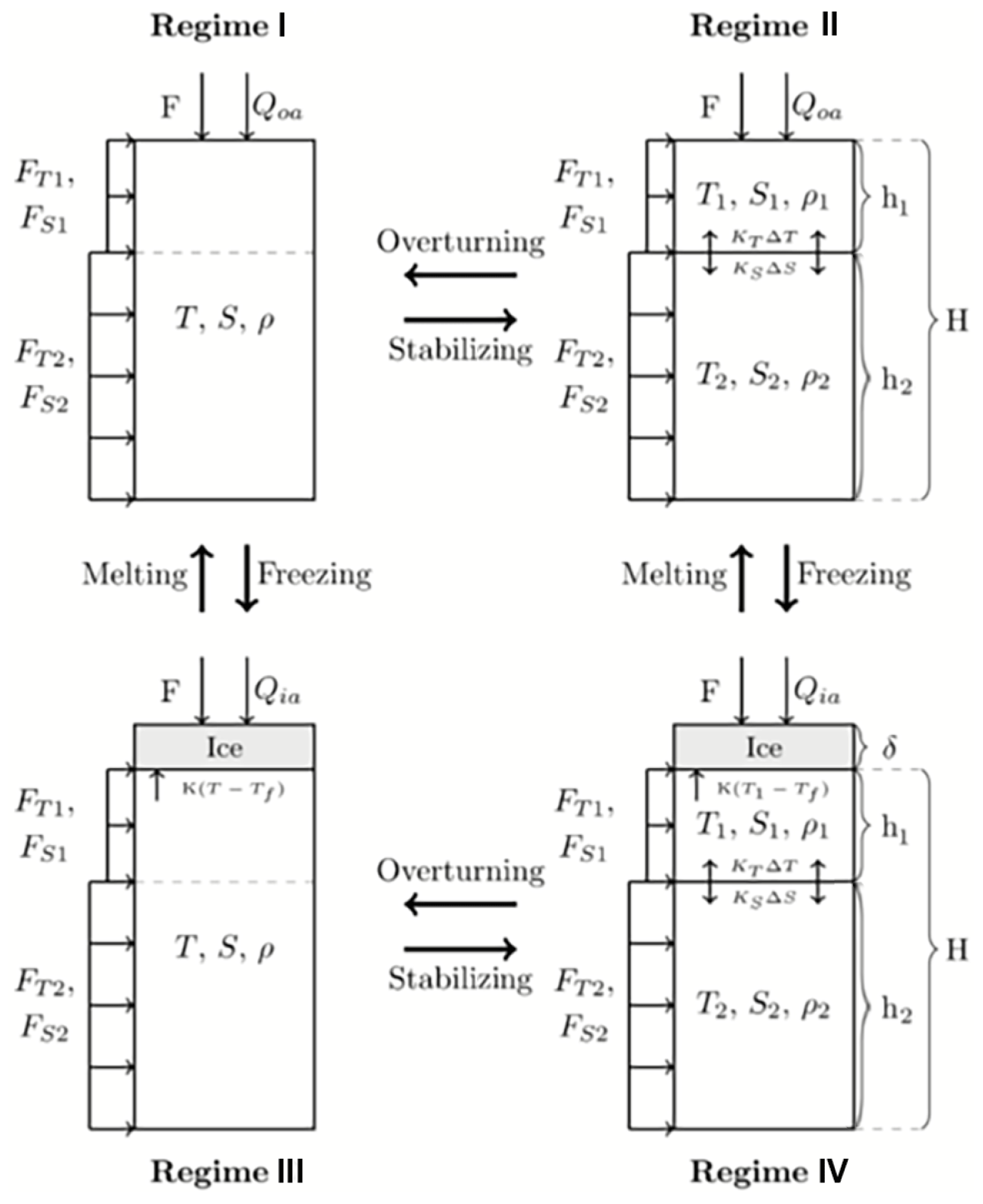
Figure 1 A schematic representation of the different regimes of the extension of the model used in Martinson et al. (1981). The parameters displayed in the figure are explained in the text. The directions and size of the arrows are not necessarily a representation of the actual direction and magnitude of the fluxes. The actual size and direction are dependent on the state of the model. Positive fluxes represent fluxes entering the water column. Regime transitions are shown by bold arrows.

The model is forced at the surface by a freshwater flux F and by a heat flux Q_ia for sea-ice-covered regimes and Q_oa for open-ocean regimes. The freshwater flux F is modeled as a virtual salt flux by multiplying it by a base salinity S₀. Both the surface and subsurface layer are subject to horizontal advective heat and salt fluxes (F_T1 and F_S1 for the surface layer, and F_T2 and F_S2 for the subsurface layer) which depend on a background value (T_b1 and S_b1 for the surface layer, and T_b2 and S_b2 for the subsurface layer) and a relaxation timescale (τ).

The heat and salt transfer between the layers are modeled using exchange coefficients (K_T and K_S), which account for upwelling, turbulent exchange, and diffusion. In sea-ice-covered regimes there is a heat flux present between the sea ice and the underlying layer. This heat flux is modeled using a turbulent exchange coefficient (K). Brine is rejected during sea-ice growth and freshwater is added to the surface layer during sea-ice melt, and brine rejection and sea-ice melt are modeled using a constant representing the salinity difference between sea ice and seawater (σ) and the rate of sea-ice growth ($\mathrm{d}\mathit{\delta }/\mathrm{d}t$). The density for each layer is determined from a simple linear equation of state:

$$\begin{array}{}\text{(1)}& \mathit{\rho }={\mathit{\rho }}_{\mathrm{0}}(\mathrm{1}-\mathit{\alpha }T+\mathit{\beta }S),\end{array}$$

where the constants α and β are the thermal expansion and haline contraction coefficients, respectively.

The governing equations for each regime are then as follows:

•  

  regime I –

  $$\begin{array}{}\text{(2a)}& {\displaystyle }H{\displaystyle \frac{\mathrm{d}T}{\mathrm{d}t}}={\displaystyle \frac{Q_{\mathrm{oa}}}{{\mathit{\rho }}_{\mathrm{0}}{C}_p}}+\mathit{\tau }(T_{\mathrm{b}\mathrm{1}}-T)h_{\mathrm{1}}+\mathit{\tau }(T_{\mathrm{b}\mathrm{2}}-T)h_{\mathrm{2}}\text{(2b)}& {\displaystyle }H{\displaystyle \frac{\mathrm{d}S}{\mathrm{d}t}}=-F{S}_{\mathrm{0}}+\mathit{\tau }(S_{\mathrm{b}\mathrm{1}}-S)h_{\mathrm{1}}+\mathit{\tau }(S_{\mathrm{b}\mathrm{2}}-S)h_{\mathrm{2}}\text{(2c)}& {\displaystyle }\mathit{\delta }=\mathrm{0};\end{array}$$
•  

  regime II –
  

  $$\begin{array}{}\text{(3a)}& {\displaystyle }{h}_{\mathrm{1}}{\displaystyle \frac{\mathrm{d}{T}_{\mathrm{1}}}{\mathrm{d}t}}={\displaystyle \frac{Q_{\mathrm{oa}}}{{\mathit{\rho }}_{\mathrm{0}}{C}_p}}+K_T(T_{\mathrm{2}}-T_{\mathrm{1}})+\mathit{\tau }(T_{\mathrm{b}\mathrm{1}}-T_{\mathrm{1}})h_{\mathrm{1}}\text{(3b)}& {\displaystyle }{h}_{\mathrm{1}}{\displaystyle \frac{\mathrm{d}{S}_{\mathrm{1}}}{\mathrm{d}t}}=K_S(S_{\mathrm{2}}-S_{\mathrm{1}})-F{S}_{\mathrm{0}}+\mathit{\tau }(S_{\mathrm{b}\mathrm{1}}-S_{\mathrm{1}})h_{\mathrm{1}}\text{(3c)}& {\displaystyle }\mathit{\delta }=\mathrm{0}\text{(3d)}& {\displaystyle \frac{\mathrm{d}{T}_{\mathrm{2}}}{\mathrm{d}t}}=\mathit{\tau }(T_{\mathrm{b}\mathrm{2}}-T_{\mathrm{2}})+{\displaystyle \frac{K_T(T_{\mathrm{1}}-T_{\mathrm{2}})}{h_{\mathrm{2}}}}\text{(3e)}& {\displaystyle \frac{\mathrm{d}{S}_{\mathrm{2}}}{\mathrm{d}t}}=\mathit{\tau }(S_{\mathrm{b}\mathrm{2}}-S_{\mathrm{2}})+{\displaystyle \frac{K_S(S_{\mathrm{1}}-S_{\mathrm{2}})}{h_{\mathrm{2}}}};\end{array}$$
•  

  regime III –
  

  $$\begin{array}{}\text{(4a)}& {\displaystyle }\begin{array}{rl}H{\displaystyle \frac{\mathrm{d}T}{\mathrm{d}t}}& =K(T-T_{\mathrm{f}})+\mathit{\tau }(T_{\mathrm{b}\mathrm{1}}-T)h_{\mathrm{1}}\\ & +\mathit{\tau }(T_{\mathrm{b}\mathrm{2}}-T)h_{\mathrm{2}}\end{array}\text{(4b)}& {\displaystyle }\begin{array}{rl}H{\displaystyle \frac{\mathrm{d}S}{\mathrm{d}t}}& =\mathit{\sigma }{\displaystyle \frac{\mathrm{d}\mathit{\delta }}{\mathrm{d}t}}-F{S}_{\mathrm{0}}+\mathit{\tau }(S_{\mathrm{b}\mathrm{1}}-S)h\\ & +\mathit{\tau }(S_{\mathrm{b}\mathrm{2}}-S)h_{\mathrm{2}}\end{array}\text{(4c)}& {\displaystyle \frac{\mathrm{d}\mathit{\delta }}{\mathrm{d}t}}={\displaystyle \frac{\mathrm{1}}{{\mathit{\rho }}_{i}L}}(-Q_{\mathrm{ia}}-{\mathit{\rho }}_{\mathrm{0}}{C}_{p}K(T-T_{\mathrm{f}}\left)\right)+{\displaystyle \frac{F{S}_{\mathrm{0}}}{\mathit{\sigma }}};\end{array}$$
•  

  regime IV –
  

  $$\begin{array}{}\text{(5a)}& {\displaystyle }\begin{array}{rl}{h}_{\mathrm{1}}{\displaystyle \frac{\mathrm{d}{T}_{\mathrm{1}}}{\mathrm{d}t}}& =K_T(T_{\mathrm{2}}-T_{\mathrm{1}})-K(T_{\mathrm{1}}-T_{\mathrm{f}})\\ & +\mathit{\tau }(T_{\mathrm{b}\mathrm{1}}-T_{\mathrm{1}})h_{\mathrm{1}}\end{array}\text{(5b)}& {\displaystyle }\begin{array}{rl}{h}_{\mathrm{1}}{\displaystyle \frac{\mathrm{d}{S}_{\mathrm{1}}}{\mathrm{d}t}}& =K_S(S_{\mathrm{2}}-S_{\mathrm{1}})+\mathit{\sigma }{\displaystyle \frac{\mathrm{d}\mathit{\delta }}{\mathrm{d}t}}-F{S}_{\mathrm{0}}\\ & +\mathit{\tau }(S_{\mathrm{b}\mathrm{1}}-S_{\mathrm{1}})h_{\mathrm{1}}\end{array}\text{(5c)}& {\displaystyle \frac{\mathrm{d}\mathit{\delta }}{\mathrm{d}t}}={\displaystyle \frac{\mathrm{1}}{{\mathit{\rho }}_{i}L}}(-Q_{\mathrm{ia}}-{\mathit{\rho }}_{\mathrm{0}}{C}_{p}K(T_{\mathrm{1}}-T_{\mathrm{f}}\left)\right)+{\displaystyle \frac{F{S}_{\mathrm{0}}}{\mathit{\sigma }}}\text{(5d)}& {\displaystyle \frac{\mathrm{d}{T}_{\mathrm{2}}}{\mathrm{d}t}}=\mathit{\tau }(T_{\mathrm{b}\mathrm{2}}-T_{\mathrm{2}})+{\displaystyle \frac{K_T(T_{\mathrm{1}}-T_{\mathrm{2}})}{h_{\mathrm{2}}}}\text{(5e)}& {\displaystyle \frac{\mathrm{d}{S}_{\mathrm{2}}}{\mathrm{d}t}}=\mathit{\tau }(S_{\mathrm{b}\mathrm{2}}-S_{\mathrm{2}})+{\displaystyle \frac{K_S(S_{\mathrm{1}}-S_{\mathrm{2}})}{h_{\mathrm{2}}}}.\end{array}$$

In these equations, C_p is the specific heat of seawater with a reference density ρ₀. Sea ice has a density of ρ_i and a latent heat of melting or freezing indicated by L. The standard values of all parameters used in the model are presented in Sect. 2.3.

In the temperature equations, the ocean–atmosphere and ice–ocean heat flux, horizontal advective fluxes, and heat transfer between the two layers are represented and transformed into temperature changes (in ^∘C s⁻¹). The temperature change due to the ocean–atmosphere flux is given by $\frac{Q_{\mathrm{oa}}}{{\mathit{\rho }}_{\mathrm{0}}{C}_p{h}_n}$, where h_n is either H (regimes I and III) or h₁ (regimes II and IV). The horizontal advective fluxes result in temperature changes given by τ(T_b1−T_n) (surface) and τ(T_b2−T_n) (subsurface), where T_n is either T (regimes I and III), T₁ (surface flux, regimes II and IV), or T₂ (subsurface flux, regimes II and IV). The temperature change due to the heat transfer between the sea ice and the surface layer is represented by $\frac{K(T_n-T_{\mathrm{f}})}{h_n}$, where T_n is either T or T₁ and h_n is either h₁ or H depending whether the model is in regime III or regime IV. Lastly, the term representing a temperature change due to heat transfer between the layers in regimes II and IV is given by $\frac{K_T(T_n-T_m)}{h_n}$, where n and m are either 1 or 2.

In the salinity equations the freshwater flux, sea-ice melt and brine rejection, horizontal advective fluxes, and salt transfer between the two layers are represented and transformed into salinity changes (in g kg⁻¹ s⁻¹). The salinity change due to the freshwater flux is given by $\frac{F{S}_{\mathrm{0}}}{h_n}$, where h_n is either H or h₁. The horizontal advective fluxes result in salinity changes given by τ(S_b1−S_n) (surface) and τ(S_b2−S_n) (subsurface), where S_n is either S (regime I and III), S₁ (surface flux, regimes II and IV), or S₂ (subsurface flux, regimes II and IV). The salt transfer between the layers in regimes II and IV result in a salinity change given by $\frac{K_S(S_n-S_m)}{h_n}$, where n and m are either 1 or 2. Brine rejection and sea-ice melt are given by $\mathit{\sigma }\frac{\mathrm{d}\mathit{\delta }}{\mathrm{d}t}$.

The sea-ice thickness is dependent on heat transfer between the sea ice and the ocean and the atmosphere, as well as the freshwater flux on top of the ice. Heat transfer between the sea ice and the atmosphere influences the sea-ice thickness via $\frac{Q_{\mathrm{ia}}}{{\mathit{\rho }}_{i}L}$. Sea-ice growth is affected by the heat transfer between the ocean and the sea ice via $\frac{{\mathit{\rho }}_{\mathrm{0}}{C}_{p}K(T-T_{\mathrm{f}})}{{\mathit{\rho }}_{i}L}$, where T is either T or T₁. Sea-ice growth due to precipitation is given by the term $\frac{F{S}_{\mathrm{0}}}{\mathit{\sigma }}$.

The set of differential equations (Eqs. 2–5) is solved using the ODE15s (Ordinary Differential Equation) solver incorporated into MATLAB. The ODE15s solver is a variable-step, variable-order solver based on an algorithm by Klopfenstein (1971) using numerical differentiation formulas (NDFs) orders 1 to 5. Tolerances for the absolute and relative error are used to increase the accuracy of the model; these tolerances are set to 10⁻¹⁰ and 10⁻⁸, respectively.

2.2 CESM simulation

In this study, we use the results of the same CESM simulation of van Westen and Dijkstra (2020a) to force the MRP box model. For a full description and details on how the simulation was performed, we refer to van Westen et al. (2020). The CESM configuration has a horizontal ocean and sea-ice model resolution of 0.1^∘ (10 km). The atmospheric component has a horizontal resolution of 0.5^∘ (50 km). The ocean (atmosphere) component has 42 (30) non-equidistant depth (pressure) levels. The model was run for 300 years under year 2000 forcing conditions. For this study, we have used model output from model years 150–250, which were detrended as described in van Westen and Dijkstra (2020a).

An example of a polynya in model year 231 of the CESM simulation is shown in Fig. 2. The Maud Rise region is first completely covered with sea ice, although the sea ice is less thick in the Maud Rise region compared with the surrounding area (Fig. 2a, b). In model year 231, the polynya forms in mid-August (Fig. 2c), after which it extends to a larger polynya in November (Fig. 2d). The analysis in van Westen and Dijkstra (2020b) has indicated that polynya formation in the CESM simulation is not caused by a bias in the mean state of the CESM (Small et al., 2014) but due to deep convection initiated in the subsurface.

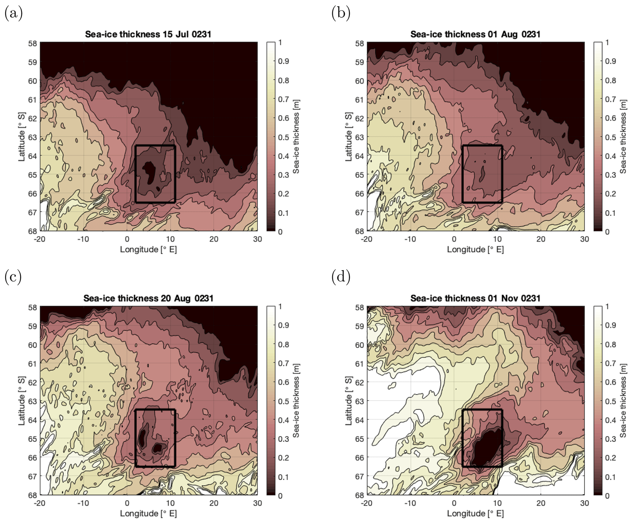
Figure 2 Daily averaged sea-ice thickness for 4 days during model year 231 when a Maud Rise polynya forms in the CESM simulation. The black outlined region represents the polynya region 2–11^∘ E × 66.5–63.5^∘ S, as defined in van Westen and Dijkstra (2020a).

2.3 MRP box model setup and case description

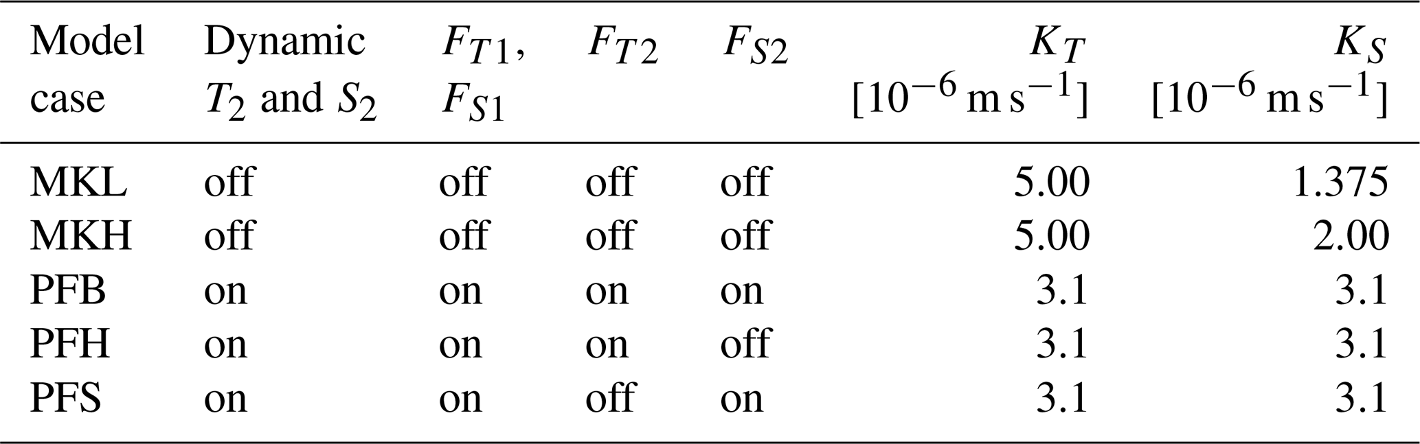
The original polynya model of Martinson et al. (1981) is obtained from the model formulation above by setting the horizontal advective fluxes (F_T1, F_S1, F_T2, and F_S2) to zero and by setting the subsurface layer values of temperature and salinity to constant values. We consider two cases of this configuration of the model, which only differ by the value of K_S used. The higher value of K_S (the MKH case, Martinson K_S high) results in more salt transfer from the subsurface layer to the surface layer (than in the MKL case, Martinson K_S low, with the lower value of K_S), thereby increasing the density of the surface layer and making it more susceptible to overturning (Table 1).

The three cases with a dynamic subsurface layer are differentiated using the inclusion of the different components of the subsurface forcing. The PFB (Periodic Flux Both) case uses both a time-varying subsurface heat and salt flux. The PFH (Periodic Flux Heat) case uses a time-varying subsurface heat flux, and the subsurface salt flux is set to a constant value. The PFS (Periodic Flux Salt) case uses a time-varying salt flux, and the heat flux is set to a constant value. The aim of this configuration is to reproduce the general features of the CESM simulation of van Westen and Dijkstra (2020a), where the observed multidecadal variability of the MRP events is one of the key features. The different cases are used to assess the importance of the different components of the subsurface forcing on the MRP formation.

Table 1 Overview of the different cases considered and values for the diffusivity parameters for heat (K_T) and salt (K_S) transfer between the two layers for each case. A model component can either be included (“on”) or excluded (“off”). The model component “dynamic T₂ and S₂” stands for an active subsurface layer. If this component is excluded, the setup uses a subsurface layer with constant density. If either F_T2 or F_S2 is excluded, the background value corresponding to the flux is set constant. The model components containing “F” represent fluxes with subscripts representing the horizontal heat (T) and salt (S) fluxes in either the surface (1) or subsurface (2) layer.

Parameter values for each case are displayed in Table 2. The parameter values are either taken from Martinson et al. (1981), are based on the CESM simulation of van Westen and Dijkstra (2020a), or are determined through tuning of the model. For the CESM simulation, we determined spatial-averaged quantities over the polynya region (2–11^∘ E × 66.5–63.5^∘ S, Fig. 2), where an MRP forms in the CESM (van Westen and Dijkstra, 2020a). The aim of the model is to investigate multiple polynya events; therefore, it is necessary to tune the stratification. The stratification can either be too strong and no overturning occurs or it can be too weak, and the water column overturns each year. To obtain multiple polynya events, the heat and salt fluxes between the two layers and between the sea ice and the surface layer are tuned.

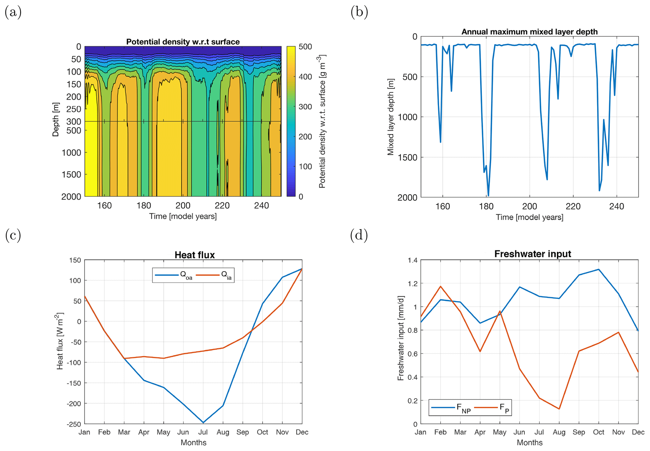
Figure 3 (a) Potential density over depth for model years 150–250 from the CESM simulation; the time series are smoothed through a 5-year running mean. (b) The annual maximum mixed layer depth for model years 150–250 from the CESM simulation. (c) The heat fluxes (in W m⁻²; see also Table 3) are determined from the CESM simulation. These values are interpolated linearly in the model as displayed in this figure. (d)  The freshwater input (in mm d⁻¹; see also Table 3) is determined from the CESM simulation. All quantities are spatially averaged over the polynya region (2–11^∘ E × 66.5–63.5^∘ S, Fig. 2).

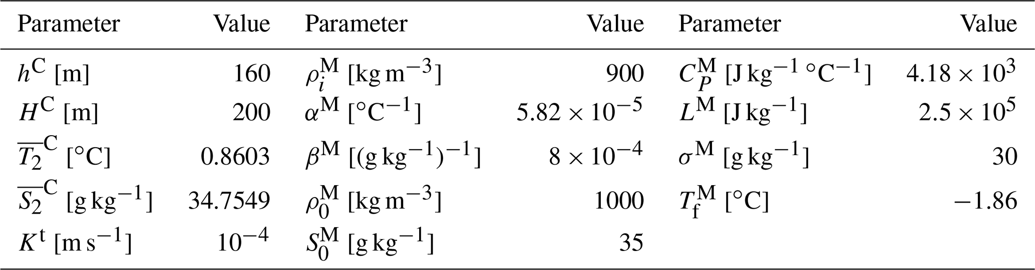
The typical depth of the layers has been determined from the CESM simulation of van Westen and Dijkstra (2020a). The depth of the surface layer (h₁) is set to 160 m, because the potential density shows a clear homogeneous layer below 160 m (Fig. 3a). This compares well to the value used in Kurtakoti et al. (2018) (h₁=150 m) but is smaller than the value used in Martinson et al. (1981) (h₁=200 m). The depth of the entire layer (H) is set to 2000 m. This is the approximate mixed layer depth during convective events in the CESM simulation (Fig. 3b). This magnitude corresponds well to values presented in Fahrbach et al. (2011) for the lower limit of where Weddell Sea Deep Water is found as well as values in Dufour et al. (2017) for the depth of the subsurface layer. It is, however, half the size of the value used in Martinson et al. (1981) (H=4000 m). The MKL and MKH cases use different subsurface temperature and salinity values. These values are the time-mean temperature and salinity of the subsurface forcing (shown in Sect. 3.1 and as dashed lines in Fig. 4) in the PFB, PFH, and PFS cases. The values used are T₂=1.175 ^∘C and S₂=34.7847 g kg⁻¹, where Martinson et al. (1981) use T₂=0 ^∘C and S₂=34.66 g kg⁻¹.

The turbulent exchange coefficient K and the exchange coefficients K_T and K_S have been used as tuning parameters for the different cases. The coefficient K is set to $\mathrm{1}\times {\mathrm{10}}^{-\mathrm{4}}$ m s⁻¹ for all cases (in Martinson et al., 1981, this value is $\mathrm{3}\times {\mathrm{10}}^{-\mathrm{4}}$ m s⁻¹). The values of K_T and K_S per case are shown in Table 1. To compare the magnitude of these parameters with values used in literature, the values need to be converted from meters per second (m s⁻¹) to meters squared per second (m² s⁻¹), which is the usual unit for vertical diffusivity parameters. This is done by multiplying these values by the depth of the surface layer (i.e., 160 m). This results in values between $\mathrm{2.2}\times {\mathrm{10}}^{-\mathrm{4}}$ and $\mathrm{5}\times {\mathrm{10}}^{-\mathrm{4}}$ m² s⁻¹. Comparable values are found in the model study of Dufour et al. (2017) for this same location and in observations (Shaw and Stanton, 2014). The values used in this study are up to a factor of 10 larger than the values used in Martinson et al. (1981) ($K_T=\mathrm{7}\times {\mathrm{10}}^{-\mathrm{7}}$ m s⁻¹ and $K_S={\mathrm{10}}^{-\mathrm{7}}$ m s⁻¹).

Table 2 Standard parameter values used in the model. Superscripts show whether the parameter value is determined from the CESM simulation of van Westen and Dijkstra (2020a) (C), determined through tuning (t), or taken from Martinson et al. (1981) (M). Overbars represent mean values (averaged over a 25-year cycle).

Initial conditions of the model affect the long-term behavior of the model. Moreover, the initial regime of the model should match with initial conditions; for example, when starting in a sea-ice-covered regime, the initial conditions for sea ice should be δ>0. Another important initial condition is the initial stratification. If the initial stratification is too weak, the model will overturn each year. In this specific case, it is not possible to study multidecadal variability in polynya formation. Therefore, each model simulation is initiated on 1 January with the following conditions: T₁=0.1 ^∘C, S₁=34.2 g kg⁻¹, and δ=1 m.

3 Results

In Sect. 3.1, the forcing conditions of the MRP box model, as determined from the CESM simulation, are discussed. Section 3.2 presents an analysis of the general model behavior, with the MKL and MKH cases being discussed in Sect. 3.3. The results for the PFB, PFH, and PFS cases are shown in Sect. 3.4. In the last section (Sect. 3.5), the effects of additive noise in the freshwater flux on the model behavior for the MKL and PFB cases are described.

3.1 Forcing conditions

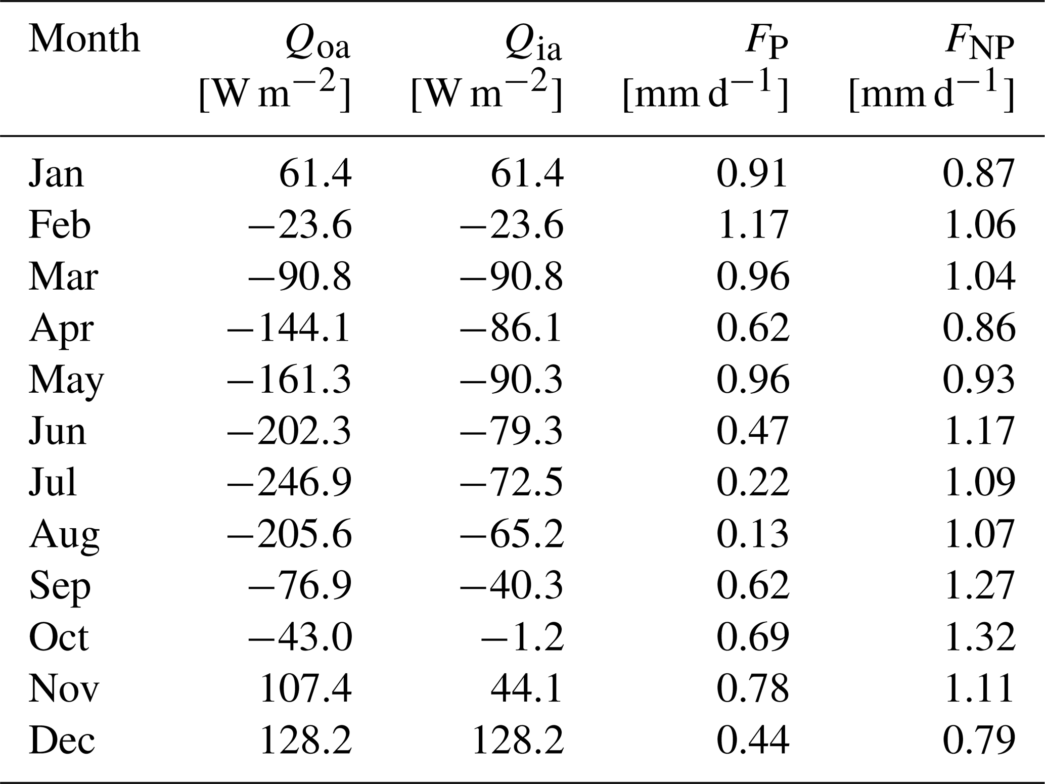
The MRP box model is forced by a monthly varying heat flux (Q_oa or Q_ia) and a monthly varying freshwater flux (F) that are repeated for each model year (Fig. 3c, d; Table 3). The monthly averaged heat fluxes are retained from the CESM. The fluxes are spatially averaged over the polynya region (2–11^∘ E × 63.5–66.5^∘ S, black outlined region in Fig. 2) defined in van Westen and Dijkstra (2020a). The surface heat flux strongly increases when the sea-ice fraction is lower than 0.5 in the CESM (not shown). Therefore, sea-ice fractions lower (higher) than 0.5 represent a sea-ice-free (sea-ice-covered) regime with the ocean–atmosphere (sea-ice–atmosphere) heat flux noted by Q_oa (Q_ia). Note that the MRP box model has a discrete sea-ice fraction of either 0 or 1. The monthly averaged heat fluxes are linearly interpolated in time. We do not use the sea-ice–ocean flux from CESM, as this flux is already represented in the model equations (e.g., by the term K(T−T_f) in Eq. 4).

There is a tendency toward more evaporation (decrease in F) when an MRP forms. Therefore, the model uses different values for the freshwater fluxes during a polynya period (F_P) and during a non-polynya period (F_NP); these freshwater fluxes are also retained from the CESM simulation, and, as for the heat fluxes, they are spatially averaged over the polynya region. The monthly averaged freshwater fluxes are also linearly interpolated in time. The yearly freshwater input is 0.38 and 0.24 m for non-polynya years and polynya years, respectively. The yearly freshwater input of F=0.38 m is within the range presented in Martinson et al. (1981) (0.38–1.73 m), although this range based on limited and outdated observations. These observations do not include polynya years; therefore, they are not necessarily representative for the freshwater input during a polynya event.

Table 3 Ocean–atmosphere heat flux (Q_oa; in W m⁻²), sea-ice–atmosphere heat flux (Q_ia; in W m⁻²), and the freshwater input ($F=P-E$; in mm d⁻¹) for polynya (P) and non-polynya (NP) regimes per month determined from the CESM simulation of van Westen and Dijkstra (2020a). Positive values represent fluxes going into the ocean or the sea ice (warming and net precipitation). Negative values represent fluxes going to the atmosphere (cooling and net evaporation). All fluxes retained from the CESM simulation are spatially averaged over 2–11^∘ E × 66.5–63.5^∘ S.

Values for the four horizontal advective fluxes (F_T1, F_S1, F_T2, and F_S2), background temperatures (T_b1 and T_b2), and salinities (S_b1 and S_b2) are obtained from the CESM simulation. The first layer uses a constant background temperature ($T_{\mathrm{b}\mathrm{1}}=-\mathrm{0.33}$^∘C). The constant background salinity (S_b1) for the surface layer is slightly changed to tune the model (from 34.5 to 34.4818 g kg⁻¹). This is necessary to be able to simulate multiple polynya events. In the CESM, the background temperature and salinity of the subsurface layer (200–1000 m depths) are periodically varying, as shown in Fig. 4. The dominant period in CESM is 25 years (not shown). This translates into a prescribed 25-year cycle for F_T2 and F_S2. The time mean values of T_b2 and S_b2 are also shown in Fig. 4. The effect of stratified Taylor columns are assimilated in the subsurface temperature and salinity time series.

These horizontal fluxes are used to make sure the water masses in the box do not drift away from the surrounding water masses. We have used fitted background states, as we are using a highly idealized model incapable of reproducing the CESM simulation accurately. Using a fitted background makes it possible to test high level hypotheses with this model. All of the horizontal fluxes are dependent on a relaxation timescale (τ), which is based on the advective timescale of the Weddell Gyre (${\mathit{\tau }}_{\mathrm{A}}=L/U$). The typical velocity scale in the Weddell Gyre is on the order of $\mathrm{5}\times {\mathrm{10}}^{-\mathrm{2}}$ m s⁻¹ (Klatt et al., 2005), and the typical length scale of the Weddell Gyre is 10⁶ m. This results in an advective timescale of 230 d. To be able to represent multiple MPR events in the model, τ is chosen as (tuned to) $\mathrm{1}/\mathrm{200}$ d.

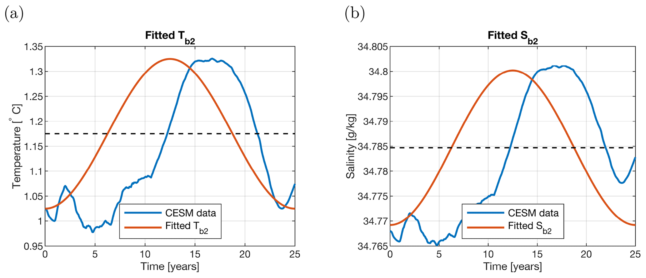
Figure 4 (a) Subsurface background temperature (T_b2) (red) used in the extended model setup fitted to model years 206–231 of the CESM simulation of van Westen and Dijkstra (2020a) (blue). The CESM simulation model output (blue line) is averaged over depth (200–1000 m) and smoothed through a 5-year running mean. The black dashed line represents the time mean used in MKL and MKH. Panel (b) is the same as panel (a) but for the subsurface background salinity (S_b2). The CESM data are spatially averaged over the 11–12^∘ E × 63.5–66.5^∘ S region, which is upstream of the polynya region defined in van Westen and Dijkstra (2020a).

3.2 Yearly repeated cycles

The MRP box model displays three types of yearly cycles, which are shown schematically in Fig. 5 for the surface box temperature and salinity. Note that the salinity axis has no values. If actual values would have been used, the cycles would overlap (see, e.g., Fig. 7c). In Fig. 5, each cycle starts at “A” and follows in alphabetical order where each letter stands for a regime transition. We use the following definition for MRP formation in this box model: an MRP has formed when the sea ice has melted away completely while there is still ocean cooling (negative heat flux).

For the no overturn (0-overturn) cycle, the model cycles between regime II (stable, sea-ice-free regime) and IV (stable, sea-ice-covered regime). At “A”, the model transits from regime II → IV because the surface layer reaches the freezing temperature. During sea-ice growth, brine is rejected, resulting in an increase in the surface salinity. During austral spring, the sea ice melts leading to an increase in the freshwater flux and a consequent decrease in salinity levels. At “B”, the model transits back to regime II as all of the sea ice has melted. Next, the surface layer temperature T₁ is mainly controlled by the atmospheric heat flux, which is positive (negative) during austral summer (autumn). When the model is cooled down to freezing temperatures, the model transits in “A” to regime IV and the (seasonal) cycle continues.

For the one overturn (1-overturn) cycle, where the model overturns once, the surface layer also reaches freezing temperatures in “A” and brine is rejected. The difference here is that the water column becomes statically unstable (ρ₁≥ρ₂) in “B” and enters the overturning regime III (mixed, sea-ice-covered regime) for a relatively short period (on the order of minutes) after which in transits back to regime IV in “C”. Due to vertical mixing, relatively warm and saline subsurface water is mixed upwards and melts the sea ice; a polynya forms. During polynya formation, the model transits to regime II in “D”. Similar to the 0-overturn cycle, the surface layer is controlled by the atmospheric heat flux for the remaining part of the year (austral winter–autumn). This cycle is similar to the one reported in Martinson et al. (1981).

For the two overturn (2-overturn) cycle, the model transits through all four regimes. The first part of the cycle (A–D) is similar to the 1-overturn cycle and a polynya forms in “D”, but considerably less sea ice forms between “A” and “B” compared with the 1-overturn cycle. After “D”, the surface layer is cooled during austral winter, but the difference here is that the surface layer becomes statically unstable in “E” and switches to regime I (mixed, sea-ice-free regime). After the model state becomes statically stable in “F”, it stays stable for the remaining part of the year.

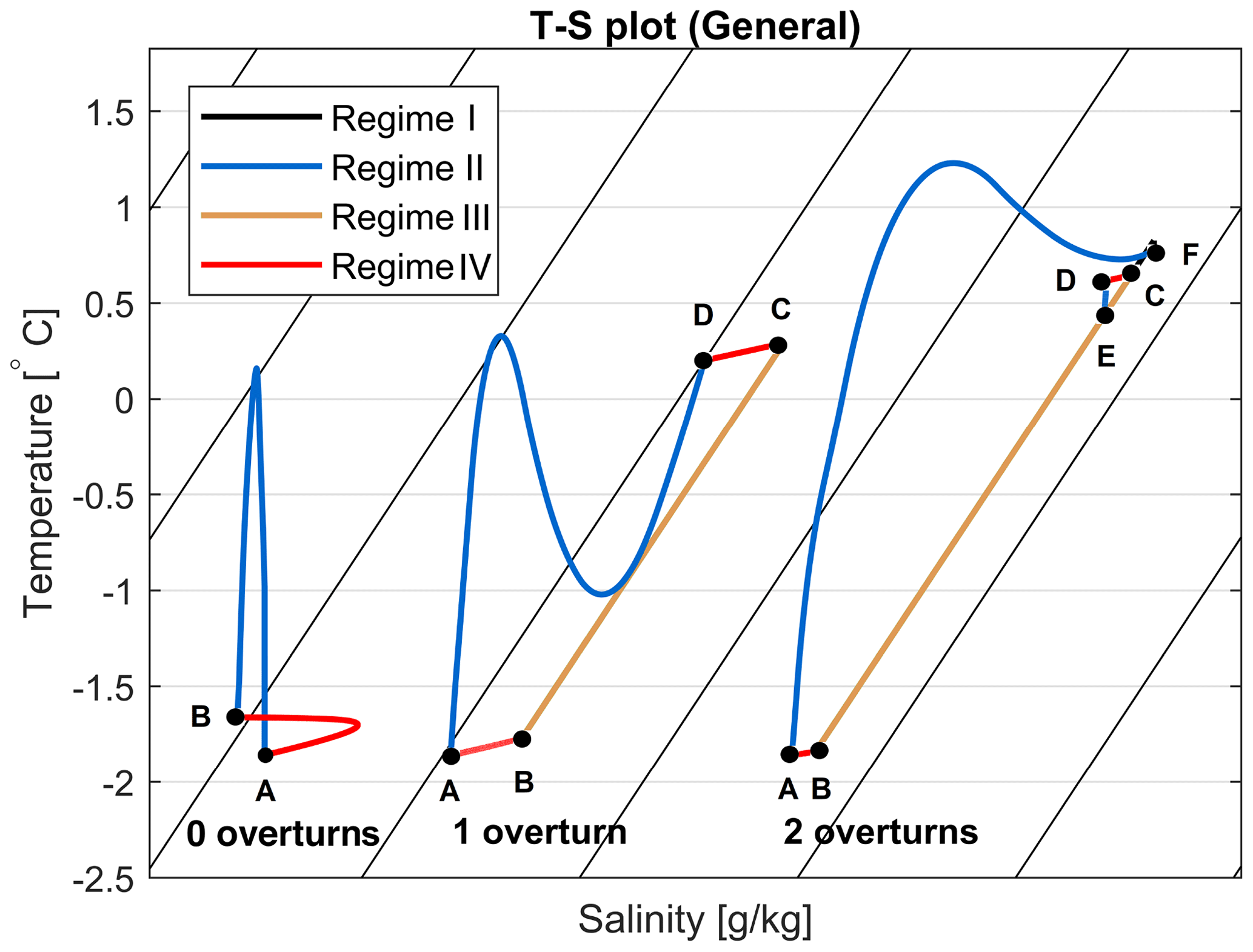
Figure 5 Schematic T₁–S₁ diagram with arbitrary scale on the salinity axis increasing to the right, showing three general cycles: no overturns (0-overturns; left), one overturn (1-overturn; middle), and two overturns (2-overturns; right) each year. The different model regimes are displayed in black (I), blue (II), orange (III), and red (IV). The letters (A–F) represent regime changes. The cycle starts at A and follows the alphabetical order. The black contours represent isopycnals, and density increases from left to right. No values are used on the salinity axis for clarity (as otherwise the cycles would overlap).

3.3 The MKL and MKH cases

When the MRP box model was configured with parameter values and numerical schemes as reported in Martinson et al. (1981), their results could not be reproduced. Unfortunately, there is an incomplete parameter documentation in Martinson et al. (1981). In addition, it is not clear how the atmospheric heat fluxes were interpolated in time. For the MKL and MKH cases (for which parameters are slightly different than those in Martinson et al., 1981), the MRP box model is spun up for 75 years and continued for another 25 years (model years 76–100).

The results for the MKL and MKH cases are shown in Fig. 6a–c and d–f, respectively. For both cases, the density of both layers, the sea-ice thickness, and a T–S diagram are shown for the last 25 years. MKL remains in the 0-overturn cycle (Fig. 5), whereas a 2-overturn cycle is found in MKH (larger K_S). In Fig. 6b and e, the sea-ice thickness shows the same (yearly) cycle every year. For temperature and salinity in the surface layer this can be seen in Fig. 6c and f, indicating that there are no variations with a period larger than 1 year. In the MKH case, there is a little sea-ice growth each year followed by overturning and subsequent sea-ice melt. Using our definition of polynya formation, we find that a polynya forms each year; therefore, the MKH case can be considered as having one long polynya period. In summary, only yearly cycle solutions are found under the given forcing for both the MKL and MKH cases. Both solutions do not correspond to MRP events in observations, as no persistent MRP is found over a few years (Campbell et al., 2019).

Figure 6 Years 76–100 for the MKL (a–c; $K_S=\mathrm{1.375}\times {\mathrm{10}}^{-\mathrm{6}}$ m s⁻¹) and MKH (d–f; $K_S=\mathrm{2}\times {\mathrm{10}}^{-\mathrm{6}}$ m s⁻¹) cases. (a, d) Density of the surface (blue) and subsurface (red) layer. (b, e) Sea-ice thickness. (c, f) T–S plot of the temperature and salinity of the surface layer. The coloring of the curves represents time, ranging from year 76 (blue) to year 100 (yellow). Only the last year is visible, because previous years have the same yearly cycle. The direction in time is the same as in Fig. 5. The black contour lines represent the density (in kg m⁻³). Shading represents polynya years.

In the CESM results of van Westen and Dijkstra (2020a), the MRP reappeared every 25 years and an MRP event lasted for about 6 consecutive years. Between model years 210 and 230, prior to MRP formation, no deep convection occurred, and the region was statically stable (van Westen and Dijkstra, 2020b). The temperature and salinity of the surface layer are seasonally varying between model years 210 and 230 (Fig. 7). The surface salinity values are increasing during the 3 years (model years 228–230) before MRP formation; these relatively higher surface salinity values did not initiate deep convection near Maud Rise in the CESM (van Westen and Dijkstra, 2020b). During model years 231–237, an MRP forms in the CESM. Deep convection mixes relatively warm and salty water from subsurface depths towards the surface resulting in the temperature and salinity of the surface layer deviating from the seasonal cycle. Clearly, the MRP box model results for the MKL and MKH cases, under the CESM-derived surface forcing, cannot reproduce the CESM results as in van Westen and Dijkstra (2020a).

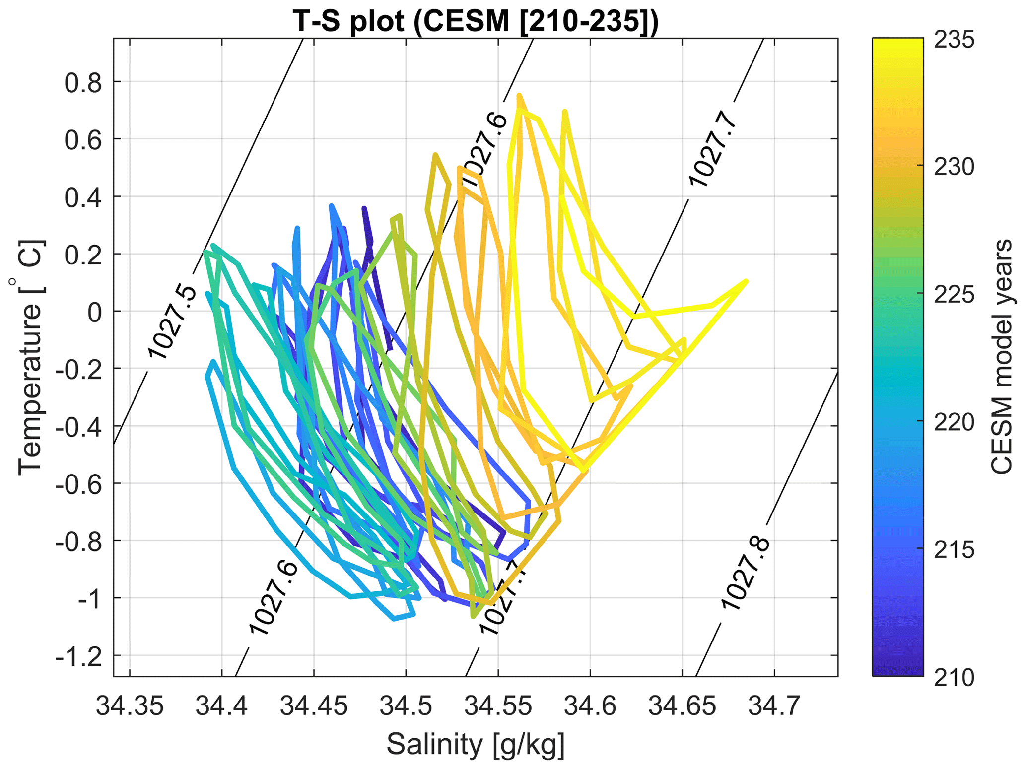
Figure 7 T–S plot of model years 210–235 from the CESM simulation (van Westen and Dijkstra, 2020a). The model is based on monthly values of the temperature and salinity averaged over the surface layer (0–160 m) over the polynya region (2–11^∘ E × 66.5–63.5^∘ S). The color coding represents time (year 210 is blue, and year 235 is yellow). The polynya period captured in this plot is between years 231 (orange) and 235 (yellow). The black contour lines represent density (in kg m⁻³), using a simple linear equation of state (Eq. 1).

3.4 The PFB, PFH, and PFS cases

For the PFB, PFH, and PFS cases, the MRP box model is spun up for 75 years and continued for another 25 years (model years 76–100). In the PFB case (Fig. 8), both heat and salt subsurface flux forcings are included. Based on the fitted subsurface fluxes (Fig. 4) and Eq. (1), the effects of the background subsurface temperature and salinity on the density almost compensate for each other. There is a relatively small subsurface density maximum between model years 87 and 88 (red line Fig. 8a). The cycle shown in Fig. 8 is repeated every 25 years, which means multidecadal recurring polynya events are simulated. Of the simulated 25 years, there are 7 polynya years and 18 non-polynya years. The polynyas are visible by reduced sea-ice maxima (mean of 0.21 m for polynya years versus a mean of 0.29 m for non-polynya years; Fig. 8b). In a 25-year cycle, the water column overturns when the subsurface density is approaching its minimum. We can also see that years with overturning can be separated by a year without overturning (e.g., in Fig. 8 there is overturning in year 76 and 78 but not in year 77). The subsurface processes also influence the characteristics of the surface layer (Fig. 8c). In the MKL and MKH cases, the yearly cycles overlap each other, but in the PFB case, the yearly cycles are different as a response to the subsurface heat and salt accumulation which is also seen in the CESM simulation (Fig. 7).

Whereas PFB uses both subsurface fluxes (heat and salt), the PFH case (Fig. 9) only uses a time-varying subsurface heat flux forcing. By thermal expansion, the subsurface density decreases and the water column becomes statically unstable in model year 86. During vertical mixing, relatively low sea-ice fractions are found compared with the stable model years. Of the simulated 25 years, there are 13 non-polynya years and 12 polynya years. Note that we do have one long polynya period here, which is different from what we see in the PFB case (Fig. 8). In the PFS case (Fig. 10), only a time-varying salt subsurface flux forcing is considered. By haline contraction, the subsurface density increases and the water column is statically stable during relatively high levels of subsurface salinity. When subsurface salinity levels decrease over time, the water column becomes unstable and a polynya forms during model years 76–84 and years 94–100. Of the simulated 25 years, there are 10 non-polynya years and 15 polynya years.

In all three cases with subsurface forcing, the MRP box model is able to simulate the general features also seen in the CESM simulation (van Westen and Dijkstra, 2020a). These cases show a repeating 25-year cycle, which is the same period as the period of the subsurface forcing and the same period as seen in CESM. Where CESM has more non-polynya years than polynya years, the PFS case has more polynya years, and the PFH case has as many non-polynya years as polynya years. However, the PFB case approaches the ratio of non-polynya years to polynya years seen in the CESM. Besides this difference, the timing of the first overturn after a non-polynya period is also different from CESM. In CESM, the first overturn occurs approximately 6 years after the subsurface heat and salt accumulation have reached their maximum. PFS overturns in approximately the same year, whereas PFB overturns 3 years later. The PFH case differs most, as it overturns 8 years earlier, which is even before the subsurface heat accumulation has reached its maximum. These differences are probably caused by the idealizations in the MRP box model and are most likely due to the representation of mixing in this model compared with that in CESM.

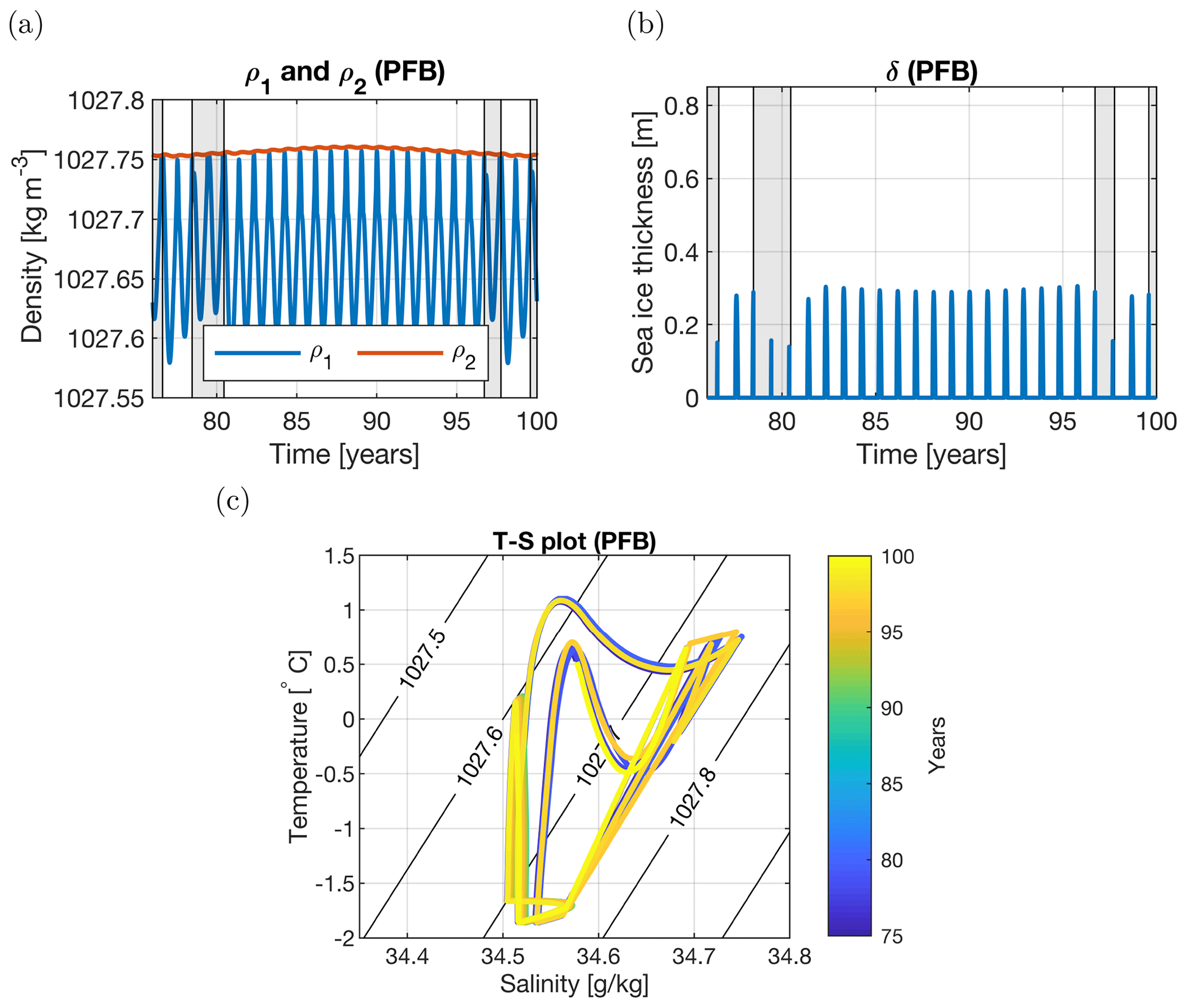
Figure 8 Years 76–100 for the PFB case (both subsurface fluxes). (a) Density of the surface (blue) and subsurface (red) layer. (b) Sea-ice thickness. The shading in panels (a) and (b) represents polynya years. (c) T–S plot of the temperature and salinity of the surface layer. The coloring of the lines represents time, ranging from year 76 (blue) to year 100 (yellow). The black contour lines represent the density (in kg m⁻³). Polynyas are present in year 76 (blue), between years 78 and 81 (blue to cyan), between years 96 and 97 (orange), and in year 99 (yellow).

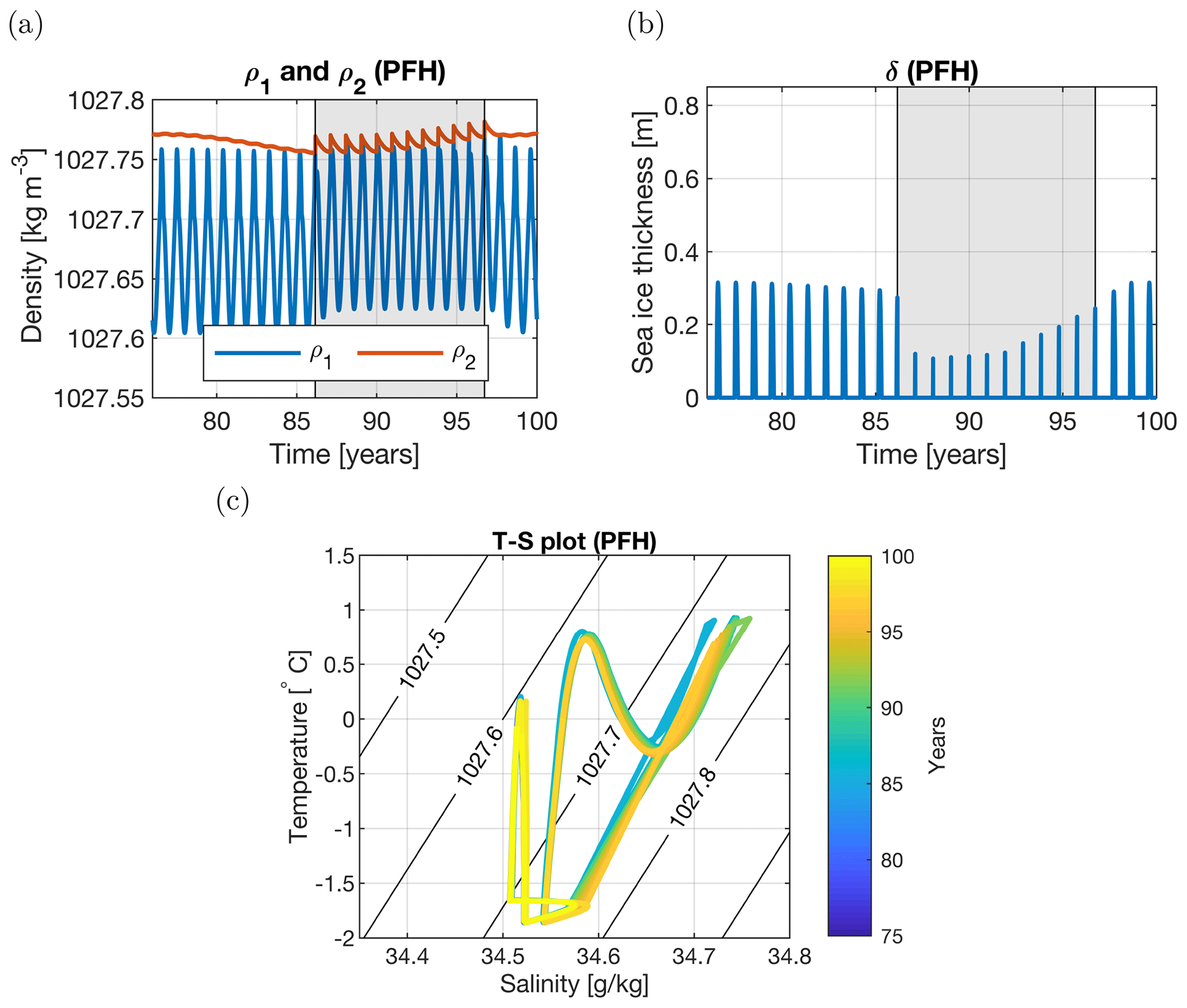
Figure 9 Years 76–100 for the PFH case (with only a subsurface heat flux). (a) Density of the surface (blue) and subsurface (red) layer. (b) Sea-ice thickness. The shading in panels (a) and (b) represents polynya years. (c) T–S plot of the temperature and salinity of the surface layer. The coloring of the lines represents time, ranging from year 76 (blue) to year 100 (yellow). The black contour lines represent the density (in kg m⁻³). Polynyas are present between year 86 (cyan) and year 96 (orange).

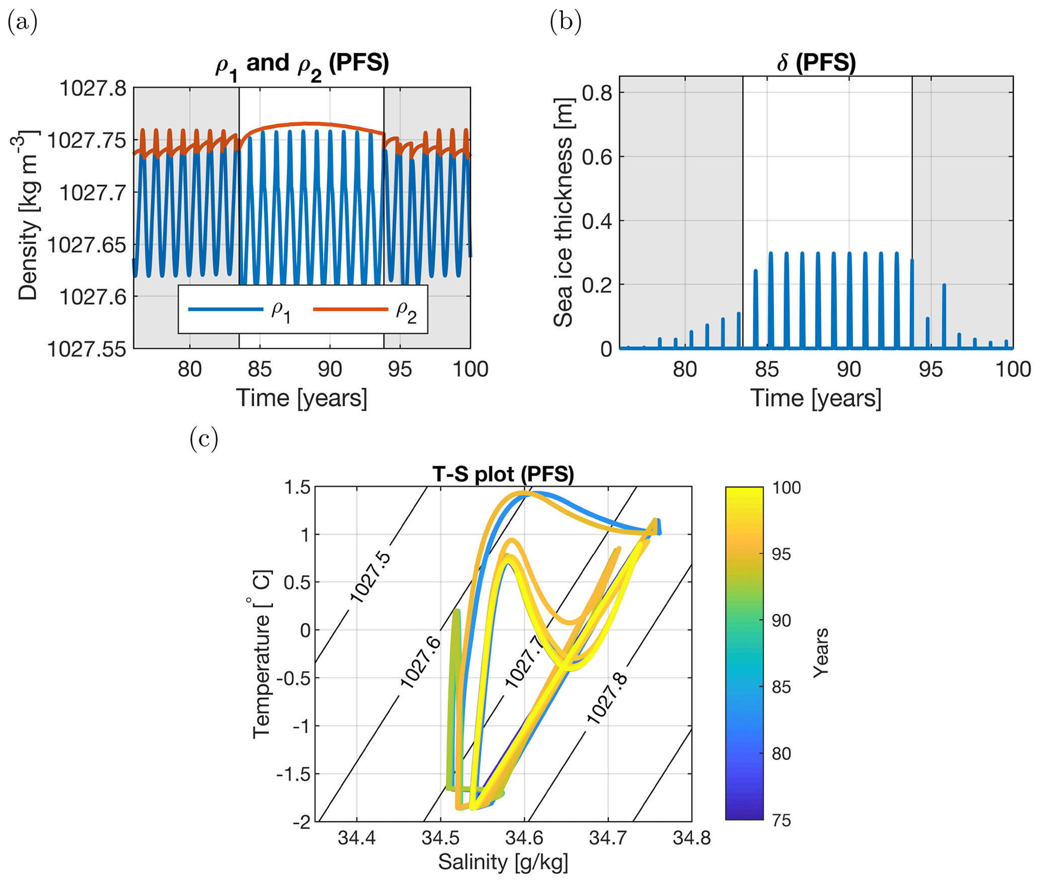
Figure 10 Years 76–100 for the PFS case (with only a subsurface salt flux). (a) Density of the surface (blue) and subsurface (red) layer. (b) Sea-ice thickness. The shading in panels (a) and (b) represents polynya years. (c) T–S plot of the temperature and salinity of the surface layer. The coloring of the lines represents time, ranging from year 76 (blue) to year 100 (yellow). The black contour lines represent the density (in kg m⁻³). Polynyas are present between year 76 (blue) and 83 (cyan) as well as after year 94 (orange to yellow).

3.5 Atmospheric variability

In this section, we analyze whether the multidecadal MRP variability, as found for the PFB, PFH, and PFS cases, is robust under the influence of atmospheric variability, such as intense winter storms. This atmospheric variability is incorporated into the MRP box model by adding white noise to the surface freshwater flux. White noise was added as in Eq. (6):

$$\begin{array}{}\text{(6)}& F_{\mathrm{N}}\left(t\right)=F\left(t\right)+{\mathit{\sigma }}_{\mathrm{N}}r\left(t\right),\end{array}$$

where F_N is the freshwater flux with noise, F is the freshwater input without noise as in Fig. 3d, σ_N is the standard deviation of the noise (0.6613 mm d⁻¹), and r is a random draw from a standard normal distribution on every time step. The standard deviation of the noise was determined from the CESM simulation.

Figure 11 displays the spectral power of the variables T₁ (Fig. 11a), S₁ (Fig. 11b), and δ (Fig. 11c) for the PFB case. For all variables, the percentile, mean, and median, the dominant period is about 25 years, which is the same period as the subsurface forcing and is clearly visible in all variables (Fig. 11a). The single ensemble member also displays a dominant period of approximately 10 years, showing that the noise can also induce shorter periods of convection. Using the same white noise forcing in the MKL case yields no dominant multidecadal period (not shown). As was seen in Sect. 3.3, the MKL case remains in 0-overturn cycle without polynyas (Fig. 6). Atmospheric noise can cause polynyas in the MKL case. However, when MKL is forced into a polynya state, it cannot be forced out of the polynya state; a polynya forms every year. This means MKL with noise will in time show the same behavior as MKH without noise. The combination of PFB and MKL shows that atmospheric variability can alter the timing of polynya formation, but the dominant period is set by subsurface fluxes of heat and salt.

Figure 11 Spectral analysis for variables (a) T₁, (b) S₁, and (c) δ for the PFB case (both subsurface fluxes). The analysis is based on 100 ensemble members. Each ensemble member contains the last 75 years of a 100-year run to exclude spin-up effects. The red band represents the ensemble members between the 10th and 90th percentile. The mean (blue), median (black), and a single ensemble member (green) are also displayed. Both axes are on a log scale. The top x axis displays the period in years, and the bottom x axis shows the frequency per year.

4 Summary and discussion

In this study, an extended version of the idealized box model of Martinson et al. (1981) was used to investigate the importance of surface forcing and subsurface forcing on Maud Rise polynya (MRP) formation, with the aim of understanding the CESM results in van Westen and Dijkstra (2020a) in more detail. The extensions in our MRP box model with respect to Martinson et al. (1981) are a dynamic subsurface layer, and horizontal subsurface heat, and salt fluxes to both the surface and the subsurface layer. Even though the results in Martinson et al. (1981) could not be reproduced exactly (due to incomplete information in the original paper), the qualitative behavior of the MRP box model (reduced to the case used in Martinson et al., 1981) was the same.

The results for the MKL and MKH cases (close to the case in Martinson et al., 1981) show that deep convection is caused by brine rejection in a preconditioned surface layer. Brine rejection causes a rapid increase in density in the surface layer. The results (Fig. 6d–f) clearly show that this eventually induces deep convection. However, brine rejection alone cannot explain observed multiple polynya events (e.g., the 1970s and 2017 events), as brine rejection is present in all years with sea-ice growth, and not all years show deep convection and subsequent polynya formation (Fig. 6a–c). In MKL, there is no overturn (Fig. 6a–c), and in the MKH case, two overturns occur each year (Fig. 6d–f). In Martinson et al. (1981), it was also shown that in time the model state will reach a yearly repeating cycle, either in regimes II (sea-ice-free, stable regime) and IV (sea-ice-covered, stable regime) (0-overturn cycle), or in regimes I (sea-ice-free, mixed regime) and II (sea-ice-free, stable regime) (2-overturn cycle). The 0-overturning case can be explained by overly strong stratification. In the MKL case, the salt transfer (governed by K_S) of the subsurface layer to the surface layer is too weak to overcome the stratification. In the second solution (two overturns each year), this salt transfer towards the surface is increased, which causes static instability in the water column with mixing as a result.

In climate models, such as CESM, the water column stabilizes after deep convection when the heat and salt reservoirs are depleted. This depletion leads to stabilization of the water column by increasing the density of the subsurface layer through heat depletion. This physical process is missing in the MKL and MKH cases; therefore, the MRP box model state is not able to return to a non-polynya regime. However, in Martinson et al. (1981), a solution was shown with overturns in the first years, after which a stable, non-polynya cycle appeared. These overturns in the first years are the result of the initial conditions. When the model is forced by the CESM surface forcing, either a polynya forms each year (MKH) or the model stays in a stable non-polynya state (MKL). Clearly, the MKL and MKH cases cannot capture the behavior of the CESM as found in van Westen and Dijkstra (2020a).

In the PFB (Fig. 8), PFH (Fig. 9), and PFS (Fig. 10) cases, subsurface forcing derived from CESM was prescribed in the MRP box model. The results showed periodic polynya events with the same dominant period as seen in van Westen and Dijkstra (2020a) caused by the periodic subsurface forcing. The subsurface forcing preconditions both the subsurface and the surface layer, after which brine rejection is essential to induce deep convection. Note that brine rejection was less important in the CESM results of van Westen and Dijkstra (2020b), as convection was initiated at the subsurface. Because this subsurface-initiated convection in CESM is spatially localized, we probably do not find it in the MRP box model. The finding of van Westen and Dijkstra (2020b) that the subsurface heat flux is more dominant than the subsurface salt flux is not confirmed in the box model, as all cases (PFB, PFH, and PFS) show comparable behavior. The subsurface heat flux, however, is expected to be dominant, as it influences every quantity (T₂, ρ₂, T₁, ρ₁, δ, S₁, S₂) in the model. The subsurface salt flux only affects the density and salinity of both layers and is, therefore, expected to have a much smaller influence on the results. Kaufman et al. (2020) also found heat buildup in the ocean and attributed this to reduced heat loss under sea-ice-covered conditions. Ocean heat advection actually seemed to counteract the heat buildup. In our model, such a situation does not occur, as T₂ is always larger than T_b2 because the subsurface layer is losing heat to the surface layer.

The MRP box model is able to capture the general features of MRP formation as seen in van Westen and Dijkstra (2020a) and shows the importance of the subsurface forcing. However, the model is still too idealized to accurately capture the precise MRP formation processes in the CESM simulation. The asymmetry in the non-polynya regime versus the polynya regime was poorly captured in the PFH and PFS cases. The asymmetry in the PFB case compared best to the CESM but still showed relatively more polynya years compared with the CESM simulation. This is probably due to the difference in how vertical mixing is represented. In the MRP box model, the layers are either in a stably stratified configuration with a constant layer depth or they are completely mixed. In van Westen and Dijkstra (2020a), a K-profile parameterization (KPP) boundary mixed layer scheme is used. Representing the growth of the mixed layer more accurately would improve the model and would possibly lead to a better representation of the asymmetry between the two regimes. When the mixed layer is allowed to grow more gradually, a lag is introduced in the system. This will delay the formation of a polynya. Due to this instant mixing, both temperature and salinity in the surface layer increase instantly. This results in large differences after overturning between the MRP box model results and the CESM simulation results (van Westen and Dijkstra, 2020a).

Martinson et al. (1981) were the first to investigate the processes responsible for polynya formation. Using their box model, they suggested that surface processes are responsible for polynya formation – a view that is still widely supported nowadays. What we have shown is that their adjusted model to the Maud Rise region is not capable of simulating multiple polynya events as seen in observations. When the model is extended with variable subsurface heat and salt accumulation, the model is capable of simulating multiple MRP events and is able to qualitatively reproduce the CESM results of van Westen and Dijkstra (2020a). Our study suggests that surface-related processes cannot completely explain MRP formation nor long-term MRP variability and that subsurface advective processes need to be taken into account.

Appendix A: Regime transitions

In the following, the conditions of the regime transitions are shown. A regime transition changes the initial conditions for the new regime. The new initial conditions are indicated with a prime. Horizontal bars above a variable represent averaging over the water column due to overturning: $\stackrel{\mathrm{‾}}{X}=(h{X}_{\mathrm{1}}+(H-h\left)X_{\mathrm{2}}\right)/H$, where X is either T or S.

$$\begin{array}{c}{\displaystyle }\text{regime I}\to \text{regime II when}-\mathit{\alpha }{\displaystyle \frac{\mathrm{d}T}{\mathrm{d}t}}+\mathit{\beta }{\displaystyle \frac{\mathrm{d}S}{\mathrm{d}t}}<\mathrm{0};\\ {\displaystyle }{T}_{\mathrm{1}}^{\prime }=T,S_{\mathrm{1}}^{\prime }=S,{\mathit{\delta }}^{\prime }=\mathrm{0},T_{\mathrm{2}}^{\prime }=T,S_{\mathrm{2}}^{\prime }=S;\\ {\displaystyle }\text{regime I}\to \text{regime III when}T=T_{\mathrm{f}};\\ {\displaystyle }{T}^{\prime }=T_{\mathrm{f}},S^{\prime }=S,{\mathit{\delta }}^{\prime }=\mathrm{0};\\ {\displaystyle }\text{regime II}\to \text{regime I when}{\mathit{\rho }}_{\mathrm{1}}={\mathit{\rho }}_{\mathrm{2}};\\ {\displaystyle }{T}^{\prime }=\stackrel{\mathrm{‾}}{T},S^{\prime }=\stackrel{\mathrm{‾}}{S},{\mathit{\delta }}^{\prime }=\mathrm{0};\\ {\displaystyle }\text{regime II}\to \text{regime IV when}{T}_{\mathrm{1}}=T_{\mathrm{f}};\\ {\displaystyle }{T}_{\mathrm{1}}^{\prime }=T_{\mathrm{1}},S_{\mathrm{1}}^{\prime }=S_{\mathrm{1}},{\mathit{\delta }}^{\prime }=\mathrm{0},T_{\mathrm{2}}^{\prime }=T_{\mathrm{2}},S_{\mathrm{2}}^{\prime }=S_{\mathrm{2}};\\ {\displaystyle }\text{regime III}\to \text{regime I when}\mathit{\delta }=\mathrm{0};\\ {\displaystyle }{T}^{\prime }=T,S^{\prime }=S,{\mathit{\delta }}^{\prime }=\mathrm{0};\\ {\displaystyle }\text{regime III}\to \text{regime IV when}-\mathit{\alpha }{\displaystyle \frac{\mathrm{d}T}{\mathrm{d}t}}+\mathit{\beta }{\displaystyle \frac{\mathrm{d}S}{\mathrm{d}t}}<\mathrm{0};\\ {\displaystyle }{T}_{\mathrm{1}}^{\prime }=T,S_{\mathrm{1}}^{\prime }=S,{\mathit{\delta }}^{\prime }=\mathit{\delta },T_{\mathrm{2}}^{\prime }=T,S_{\mathrm{2}}^{\prime }=S;\\ {\displaystyle }\text{regime IV}\to \text{regime II when}\mathit{\delta }=\mathrm{0};\\ {\displaystyle }{T}_{\mathrm{1}}^{\prime }=T_{\mathrm{1}},S_{\mathrm{1}}^{\prime }=S_{\mathrm{1}},{\mathit{\delta }}^{\prime }=\mathrm{0},T_{\mathrm{2}}^{\prime }=T_{\mathrm{2}},S_{\mathrm{2}}^{\prime }=S_{\mathrm{2}};\\ {\displaystyle }\text{regime IV}\to \text{regime III when}{\mathit{\rho }}_{\mathrm{1}}={\mathit{\rho }}_{\mathrm{2}};\\ {\displaystyle }{T}^{\prime }=\stackrel{\mathrm{‾}}{T},S^{\prime }=\stackrel{\mathrm{‾}}{S},{\mathit{\delta }}^{\prime }=\mathit{\delta };\end{array}$$