Diapycnal mixing across the photic zone of the NE Atlantic

Variable physical conditions such as vertical turbulent exchange, internal wave, and mesoscale eddy action affect the availability of light and nutrients for phytoplankton (unicellular algae) growth. It is hypothesized that changes in ocean temperature may affect ocean vertical density stratification, which may hamper vertical exchange. In order to quantify variations in physical conditions in the northeast Atlantic Ocean, we sampled a latitudinal transect along 17 ± 5^∘ W between 30 and 63^∘ N in summer. A shipborne conductivity–temperature–depth (CTD) instrumented package was used with a custom-made modification of the pump inlet to minimize detrimental effects of ship motions on its data. Thorpe-scale analysis was used to establish turbulence values for the upper 500 m from three to six profiles obtained in a short CTD yo-yo, 3 to 5 h after local sunrise. From south to north, average temperature decreased together with stratification while turbulence values weakly increased or remained constant. Vertical turbulent nutrient fluxes did not vary significantly with stratification and latitude. This apparent lack of correspondence between turbulent mixing and temperature is likely due to internal waves breaking (increased stratification can support more internal waves), acting as a potential feedback mechanism. As this feedback mechanism mediates potential physical environment changes in temperature, global surface ocean warming may not affect the vertical nutrient fluxes to a large degree. We urge modellers to test this deduction as it could imply that the future summer phytoplankton productivity in stratified oligotrophic waters would experience little alterations in nutrient input from deeper waters.

1 Introduction

The physical environment is important for ocean life, including variations therein. For example, the sun stores heat in the ocean with a stable vertical density stratification as result. Generally, stratification hampers vertical turbulent exchange because of the required work against (reduced) gravity before turbulence can take effect. It thus hampers a supply of nutrients via a turbulent flux from deeper waters to the photic zone. However, stratification supports internal waves, which (i) may move near-floating particles like phytoplankton (unicellular algae) up and down towards and away from the surface and (ii) may induce enhanced turbulence via vertical current differences (shear) resulting in internal waves breaking (Denman and Gargett, 1983). Such changes in the physical environment are expected to affect the availability of phytoplankton growth factors such as light and nutrients.

Climate models predict that global warming will reduce vertical mixing in the oceans (e.g. Sarmiento et al., 2004). Mathematical models on system stability suggest that reduced mixing may generate chaos behaviour in phytoplankton production, thereby enhancing variability in carbon export into the ocean interior (Huisman et al., 2006). However, none of these models include potential feedback systems like internal wave action or mesoscale eddy activity. From observations in the relatively shallow North Sea it is known that the strong seasonal temperature stratification is marginally stable, as it supports internal waves and shear to such extent that sufficient nutrients are replenished from below to sustain the late-summer phytoplankton bloom in the euphotic zone that became depleted of nutrients after the spring bloom (van Haren et al., 1999). This challenges the current paradigm in climate models.

In this paper, the objective is to resolve the effect of vertical stratification and turbulent mixing on nutrient supply to the euphotic zone of the open ocean. For this purpose, upper 500 m ocean shipborne conductivity–temperature–depth (CTD) observations were made in association with those on dissolved inorganic nutrients during a survey along a transect in the NE Atlantic Ocean from midlatitudes (30^∘) to high (63^∘) latitudes in summer. Throughout the survey, meteorological and sea-state conditions were favourable for adequate sampling and wind speeds varied little between 5 and 10 m s⁻¹, independent of locations. All CTD observations were made far from lateral, continental boundaries and at least 1000 m vertically away from bottom topography (i.e. far from internal-tide sources). The NE Atlantic is characterized by abundant (sub-)mesoscale eddies especially in the upper ocean (Charria et al., 2017) that influence local plankton communities (Hernández-Hernández et al., 2020). The area also shows continuous abundant internal wave activity away from topographic sources and sinks, with the semidiurnal tide as a main source from below and atmospherically induced inertial motions from above (e.g. van Haren, 2005, 2007). However, the sampled upper 500 m zone transect is not known to demonstrate outstanding internal wave source variations. Previous observations (van Haren, 2005) and Hibiya et al. (2007) have shown that a diurnal critical latitude enhancement of near-inertial internal waves due to subharmonic instability only occurs sharply between 25 and 30^∘ N. The present observations are all made poleward of this range. Likewise, the Henyey et al. (1986) model on latitudinal variation in internal wave energy and turbulent mixing (Gregg et al., 2003) predicts changes by a maximum factor of 1.8 between 30 and 63^∘, but this value is relatively small compared with errors, typically a factor of 2 to 3, in turbulence dissipation rate observations. Likewise, from the equal summertime meteorological conditions little variation is expected in the generation of upper-ocean near-inertial internal waves. Naturally, other processes like interaction between internal waves and mesoscale phenomena may be important locally, but these are expected to occur in a similar fashion across the sampled ocean far away from boundaries. Thus, the sampled dataset is considered adequate for a discussion on the variability of turbulence, stratification, and vertical turbulent nutrient fluxes with latitude.

The present research complements research based on photic zone (upper 100 m) observations obtained along the same transect using a slowly descending turbulence microstructure profiler next to CTD sampling 8 years earlier (Jurado et al., 2012). Their data demonstrated a negligibly weak increase in turbulence values with significant decreases in stratification going north. However, no nutrient data were presented and no turbulent nutrient fluxes could be computed. In another summertime study (Mojica et al., 2016), macro-nutrient concentrations indicated oligotrophic conditions along the same latitudinal transect but the vertical gradients for the upper 200 m showed an increase from south to north. The present observations go deeper to 500 m, also across the non-seasonal more permanent stratification. Moreover, coinciding measurements were made of the distributions of macro-nutrients and dissolved iron. This allows vertical turbulent nutrient fluxes to be computed. It leads to a hypothesis concerning a physical feedback mechanism that may control changes in stratification.

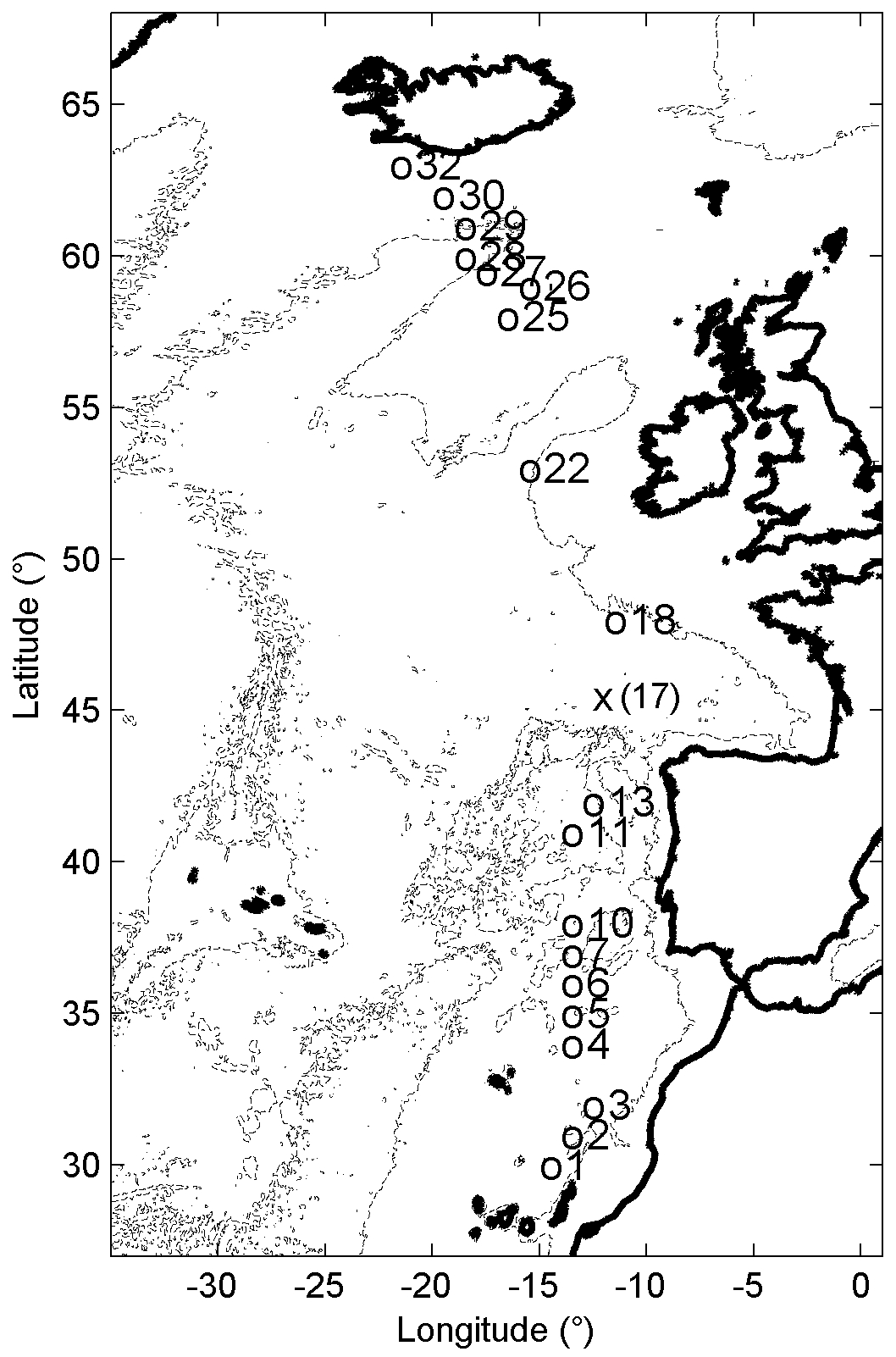
Figure 1 Bathymetry map of the northeast Atlantic Ocean based on the 9.1 ETOPO-1 version of satellite altimetry-derived data by Smith and Sandwell (1997). The numbered circles indicate the CTD stations, at station 17 (x) no turbulence parameter and only nutrient sampling were done. At stations 1 and 2 no DFe samples were taken; at station 18 no nutrient samples were taken. Depth contours are at 2500 and 5000 m.

2 Materials and methods

Between 22 July and 16 August 2017, observations were made from the R/V Pelagia in the northeast Atlantic Ocean at stations along a transect from Iceland, starting around 60^∘ N, to the Canary Islands, ending at 30^∘ N (Fig. 1). The transect was roughly in meridional direction, with stations along 17 ± 5^∘ W, all in the same time zone (UTC−1: local time LT). Full water-depth Rosette bottle water sampling was performed at most stations.

Samples for dissolved inorganic macro-nutrients were filtered through 0.2 µm Acrodisc filter and stored frozen in a high-density polyethylene pony vial (nitrate, nitrite, and phosphate) or at 4 ^∘C (silicate) until analysis. Nutrients were analysed under temperature-controlled conditions using a QuAAtro gas segmented continuous flow analyser. All measurements were calibrated with standards diluted in low-nutrient seawater in the salinity range of the stations to ensure that analysis remained within the same ionic strength. Phosphate (PO₄) and nitrate plus nitrite (NO_x) were measured according to Murphy and Riley (1962) and Grasshoff et al. (1983), respectively. Silicate was analysed using the procedure of Strickland and Parsons (1968).

Absolute and relative precision were regularly determined for reasonably high concentrations in an in-house standard. For phosphate, the SD was 0.028 µM (N = 30) for a concentration of 0.9 µM; hence the relative precision was 3.1 %. For nitrate, the values were 0.14 µM (N = 30) for a concentration of 14.0 µM, so that the relative precision was 1.0 %. For silicate, the values were 0.09 µM (N = 15) for a concentration of 21.0 µM, so that the relative precision was 0.4 %. The detection limits were 0.007, 0.012, and 0.008 µM, for phosphate, nitrate, and silicate, respectively.

For dissolved iron samples, the ultraclean “pristine” sampling system for trace metals was used (Rijkenberg et al., 2015). All bottles used for storage of reagents and samples were cleaned according to an intensive three-step cleaning protocol described by Middag et al. (2009). Dissolved iron concentrations were measured shipboard using a flow-injection–chemiluminescence method with preconcentration on iminodiacetic acid resin as described by De Baar et al. (2008) and modified by Klunder et al. (2011). In order to validate the accuracy of the system, standard reference seawater (SAFe) was measured regularly in triplicate (Johnson et al., 1997).

At 19 out of 32 stations a yo-yo consisting of three to six casts, totaling 88 casts, of electronic CTD profiles was done to monitor the temperature–salinity variability and to establish turbulent mixing values from 5 to 500 m below the ocean surface. For the yo-yos a separate CTD instrument was used from the CTD ultraclean sampling system. The yo-yo casts were made consecutively and took between 1 and 2 h per station. They were mostly obtained in the morning: at 10 stations between 06:00 and 08:00 LT, at 8 stations between 08:00 and 10:00 LT, and at 1 station around noon. As the observations were made in summer, the latitudinal difference in sunrise was 1.5 h between the northernmost (earlier sunrise) and southernmost stations. This difference is taken into account and sampling times are referenced to time after local sunrise. It is assumed that the stations sampled just after sunrise reflect the upper-ocean conditions of (late-) nighttime cooling convection so that vertical near-homogeneity was at a maximum and near-surface stratification at a minimum, while the late morning and afternoon stations reflected daytime stratifying near-surface conditions due to the stabilizing solar insolation.

2.1 Instrumentation and modification

Calibrated SeaBird 911plus CTD instruments were used. The CTD data were sampled at a rate of 24 Hz, whilst lowering the instrumental package at an average speed of 0.9 m s⁻¹. The yo-yo CTD data were processed using the standard procedures incorporated in the SBE software, including corrections for cell thermal mass (Lueck, 1990) using the parameter setting of Mensah et al. (2009), sensor time alignment and vertical bin averaging over 0.33 m. All other analyses were performed using Conservative Temperature (Θ), Absolute Salinity S_A, and potential density anomalies σ_θ, with 1000 kg m⁻³ subtracted from total density and referenced to the surface for pressure corrections as only vertical profiles shallower than 600 m were analysed, using the Gibbs SeaWater software (IOC, SCOR, IAPSO, 2010).

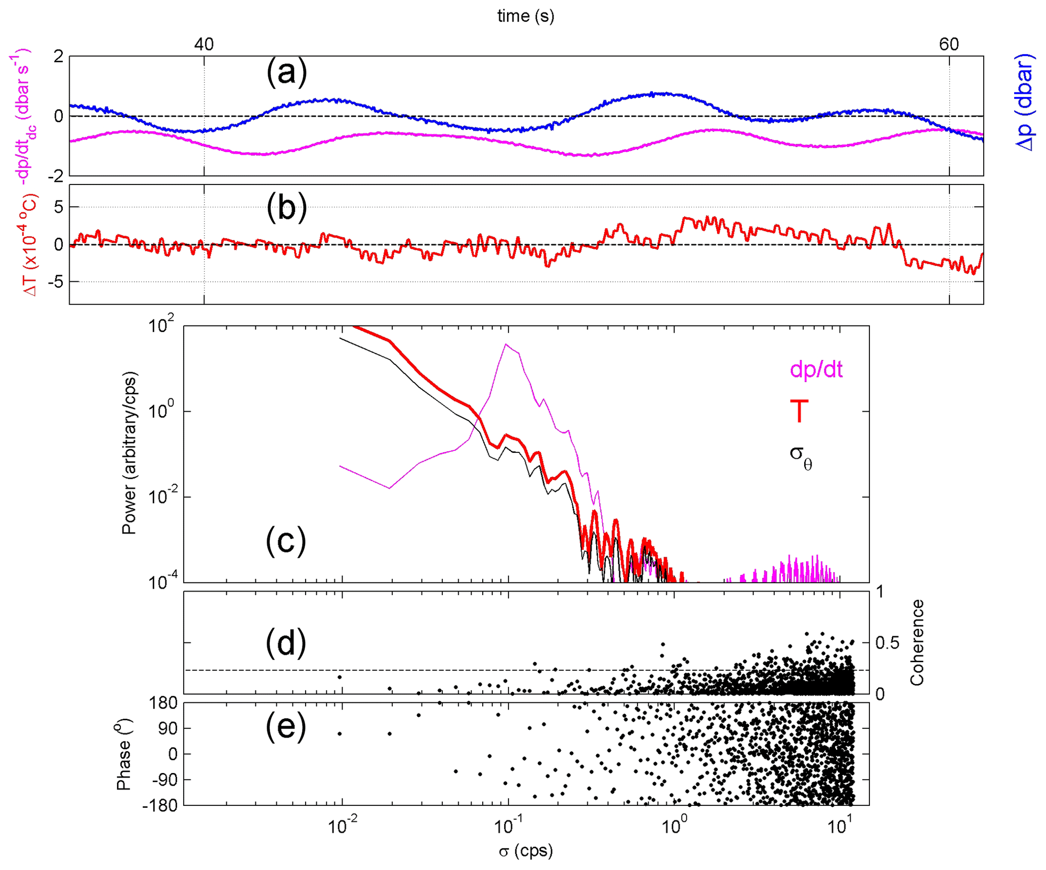
Figure 2 Test of effective removal of ship motions in CTD data after pump in- and outlet modification. Nearly raw 24 Hz sampled downcast data obtained from northern station 32 (cast 9). Short example time series for the 20 m depth range [10, 30] m. (a) Detrended pressure (blue) and its (negative signed) first time derivative $-\mathrm{d}p/\mathrm{d}t$, 2 dbar smoothed (purple). (b) Detrended temperature. (c) Moderately smoothed (∼ 30 degrees of freedom; dof) spectra of data from the 5 to 500 m depth range. (d) Moderately smoothed (40 dof) coherence between $\mathrm{d}p/\mathrm{d}t$ and T from (c), with dashed line indicating the 95 % significance level. (e) Corresponding phase difference.

Observations were made with the yo-yo CTD instrument upright rather than horizontal in a lead-weighted frame without water samplers to minimize artificial turbulent overturning. Variable speeds of the flow passing the temperature and conductivity sensors will cause artificial temperature and thus apparent turbulent overturning, noticeable in near-homogeneous waters such as those found near the surface during nighttime convection. To eliminate variable flow speeds, a custom-made assembly with pump in- and outlet tubes and tube ends of exactly the same diameter was mounted on the CTD instrument as described in van Haren and Laan (2016). This reduces frictional temperature effects of typically ± 0.5 mK due to fluctuations in pump speed of ± 0.5 m s⁻¹ when standard SBE tubing is used (Appendix A). The effective removal of the artificial temperature effects using the custom-made assembly is demonstrated in Fig. 2, in which surface wave action via ship motion is visible in the CTD–pressure record but not in its temperature variations record. For example, at station 32 the CTD instrument was lowered in moderate sea-state conditions with maximum surface waves of 2 m crest trough. The surface waves are recorded by pressure variations as a result of ship motions (Fig. 2a). In the upper 35 m near the surface, the waters were partially unstable and partially near-homogeneous, with temperature variations well within ± 0.5 mK and high-frequency variations O(0.1) mK (Fig. 2b). The ΔT variations did not vary with the surface wave periodicity of about 10 s. No correlation was found between data in Fig. 2b and a. This effective removal of ship motion in CTD temperature data is confirmed for the entire 500 m depth range in average spectral information (Fig. 2c–e). In the power spectra, the pressure gradient $\mathrm{d}p/\mathrm{d}t$ ∼ CTD velocity shows a clear peak around 0.1 cps, short for cycles per second, which corresponds to a period of 10 s. Such a peak is absent in both spectra of temperature T and density anomaly referenced to the surface σ_θ. The correlation between $\mathrm{d}p/\mathrm{d}t$ and T is not significantly different from zero (Fig. 2d and e). With conventional tubing and tube ends, the surface wave variations would show up in such ΔT graph (van Haren and Laan, 2016). Without the effects of ship motions, considerably less corrections need to be applied for turbulence calculations (see below).

2.2 Ocean turbulence calculation

Turbulence is quantified using the analysis method by Thorpe (1977) on potential density inversions of less dense water below a layer of denser water in a vertical (z) profile. Such inversions are interpreted as turbulent overturns of mechanical energy mixing. Vertical turbulent kinetic energy dissipation rate (ε) is a measure of the amount of kinetic energy put in a system for turbulent mixing. It is proportional to the magnitude of turbulent diapycnal flux (of potential density) $\mathrm{|}{K}_z\mathrm{d}{\mathit{\sigma }}_{\mathit{\theta }}/\mathrm{d}z\mathrm{|}$. In practice it is determined by calculating overturning scales with magnitude |d|, just like turbulent eddy diffusivity (K_z). The vertical potential density stratification is indicated by $\mathrm{d}{\mathit{\sigma }}_{\mathit{\theta }}/\mathrm{d}z$. The turbulent overturning scales are obtained after reordering the measured profile σ_θ(z), which may contain inversions, into a stable monotonic profile σ_θ(z_s) without inversions (Thorpe, 1977). After comparing raw and reordered profiles, displacements d = $min(\mathrm{|}z-z_{\mathrm{s}}\mathrm{|})\cdot \text{sgn}(z-z_{\mathrm{s}})$ are calculated that generate the stable profile. Then, using root-mean-square displacement value L_T=rms(d) computed over certain vertical scales (see below):

$$\begin{array}{}\text{(1)}& \mathit{\epsilon }=\mathrm{0.64}{L}_{\mathrm{T}}^{\mathrm{2}}{N}^{\mathrm{3}}\left[{\mathrm{m}}^{\mathrm{2}}{\mathrm{s}}^{-\mathrm{3}}\right],\end{array}$$

where N = $\mathit{\{}-g/\mathit{\rho }(\mathrm{d}{\mathit{\sigma }}_{\mathit{\theta }}\left(z_{\mathrm{s}}\right)/\mathrm{d}z){\mathit{\}}}^{\mathrm{1}/\mathrm{2}}$ denotes the buoyancy frequency (∼ square root of stratification as is clear from the equation) computed from the reordered profile. Here, g is the acceleration of gravity and ρ = 1027 kg m⁻³ denotes the reference density. We like to note, following previous warnings by, e.g., Gill (1982) and King et al. (2012), that our definition of N is a practical one, which should not be used for data from deeper waters. For deeper waters, density should be referenced to a local pressure reference level, which effectively implies the use of the exact definition for buoyancy frequency as formulated by, e.g., Gill (1982): $\mathit{\{}-g/\mathit{\rho }(\mathrm{d}\mathit{\rho }/\mathrm{d}z+g\mathit{\rho }/c_{\mathrm{s}}^{\mathrm{2}}){\mathit{\}}}^{\mathrm{1}/\mathrm{2}}$, where c_s is the speed of sound reflecting pressure–compressibility effects. Our “surface waters” N computed over reordered profiles only negligibly deviates from above exact N and corresponds to N computed from raw profiles over a typical vertical length scale of Δz = 100 m. This Δz represents the scales of large internal waves that are supported by the density stratification and of the largest turbulent overturns.

The numerical constant of 0.64 in Eq. (1) follows from empirically relating the overturning scale magnitude with the Ozmidov scale L_O of the largest possible turbulent overturn in a stratified flow: ($L_{\mathrm{O}}/L_{\mathrm{T}})$ = 0.8 (Dillon, 1982) this is a mean coefficient value from many realizations. Using K_z = ΓεN⁻² and a mean mixing efficiency coefficient of Γ = 0.2 for the conversion of kinetic into potential energy for ocean observations that are suitably averaged over all relevant turbulent overturning scales of the mix of shear, current-difference-driven and convective, buoyancy-driven overturning in large Reynolds number flow conditions (e.g. Osborn, 1980; Oakey, 1982; Ferron et al., 1998; Gregg et al., 2018), we find

$$\begin{array}{}\text{(2)}& K_z=\mathrm{0.128}{L}_{\mathrm{T}}^{\mathrm{2}}N\left[{\mathrm{m}}^{\mathrm{2}}{\mathrm{s}}^{-\mathrm{1}}\right].\end{array}$$

This parametrization is also valid for the upper ocean, as has been shown extensively by Oakey (1982) and recently confirmed by Gregg et al. (2018). The inference is that the upper ocean may be weakly stratified at times, but stratification and turbulence vary considerably with time and space. Sufficient averaging collapses coefficients to the mean values given above. This is confirmed in recent numerical modelling by Portwood et al. (2019).

As K_z is a mechanical turbulence coefficient, it is not property-dependent like a molecular diffusion coefficient that is about 100-fold different for temperature compared to salinity. K_z is thus the same for all turbulent transport calculations no matter what gradient of what property. For example, the vertical downgradient turbulent flux of dissolved iron transporting from iron-rich deeper waters upwards into the euphotic zone is computed as $-K_z\mathrm{d}\left(\mathrm{DFe}\right)/\mathrm{d}z$.

According to Thorpe (1977), results from Eqs. (1) and (2) are only useful after averaging over the size of a turbulent overturn instead of using single displacements. Here, rms-displacement values L_T are not determined over individual overturns, as in Dillon (1982), but over 7 m vertical intervals (equivalent to about 200 raw data samples) that just exceed average L_O. This avoids the complex distinction of smaller overturns in larger ones and allows the use of a single length scale of averaging. As a criterion for determining overturns we only used those data of which the absolute value of difference with the local reordered value exceeds a threshold of 7 × 10⁻⁵ kg m⁻³, which comes from SDs of the potential density profiles in near-homogeneous layers over 1 m intervals and which corresponds to noise-variational amplitudes of 1.4 × 10⁻⁴ kg m⁻³ in raw data (e.g. Galbraith and Kelley, 1996; Stansfield et al., 2001; Gargett and Garner, 2008). Vertically averaged turbulence values, short for averaged ε and K_z values from Eqs. (1) and (2), can be calculated to within an error of a factor of 2 to 3, approximately. As will be demonstrated below, this is considerably less spread in values than the natural turbulence values variability over typically 4 orders of magnitude at a given position and depth in the ocean (e.g. Gregg, 1989).

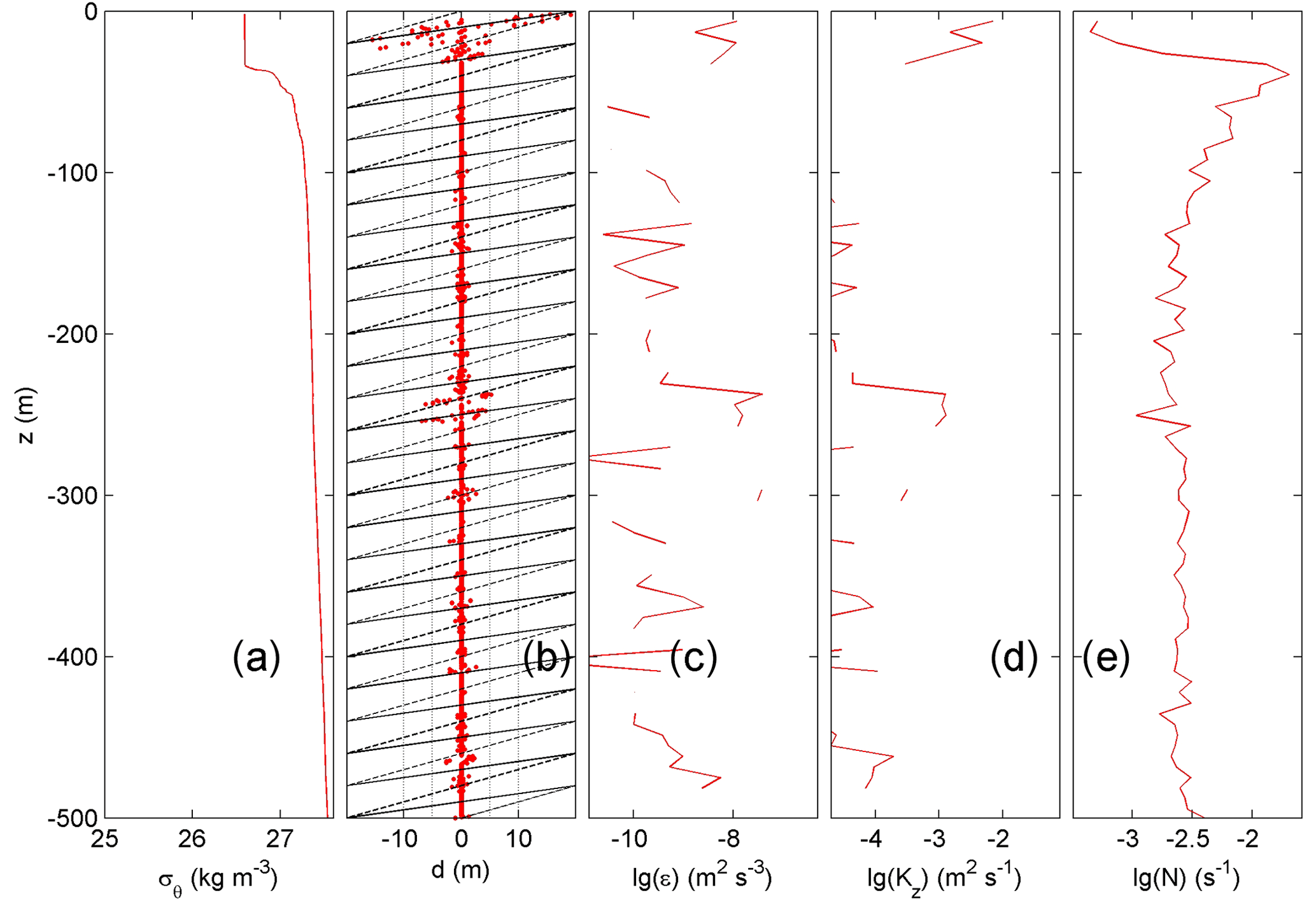
Figure 3 Upper 500 m of turbulence characteristics computed from downcast density anomaly data applying a threshold of 7 × 10⁻⁵ kg m⁻³. Northern station 29, cast 2. (a) Unordered, “raw” profile of density anomaly referenced to the surface. (b) Overturn displacements following reordering of the profiles in (a). Slopes $\mathrm{1}/\mathrm{2}$ (solid lines) and 1 (dashed lines) are indicated. (c) Logarithm of dissipation rate computed from the profiles in (a), rms calculated over 7 m intervals. We use the mathematics expression “lg” for the 10-base logarithm, as given in the ISO 80000 specification. (d) As (c), but for eddy diffusivity. (e) Logarithm of buoyancy frequency computed after reordering the profiles of (a).

3 Results

3.1 Physical parameters

An early morning vertical profile of density anomaly in the upper 500 m at a northern station (Fig. 3a) is characterized by a near-homogeneous layer of about 15 to 40 m, which is above a layer of relatively strong stratification and a smooth moderate stratification deeper below. In the near-homogeneous upper layer, in this example $z>-\mathrm{30}\mathrm{m}$, relatively large turbulent overturn displacements can be found of d =  ± 20 m (Fig.  3b): so-called large density inversions. In this paper we conventionally define “mixed layer depth” as the depth at which the temperature difference with respect to the surface is 0.5 ^∘C (Jurado et al., 2012). We note that this actually more represents the “mixing layer depth” and the reordered profile shows non-zero stratification. If the mixed-layer-depth definition had been applying a temperature difference of, e.g., 0.001 ^∘C on the reordered profile, its value would have averaged about 5 m, much less than using the present and more common, conventional definition applying a temperature difference of 0.5 ^∘C. We thus present turbulence results for this commonly defined “mixed layer” with caution, whilst observing their consistency with the results from deeper down, as presented below. For −200 < z < −30 m, large turbulent overturns are few and far between. Turbulence dissipation rate (Fig. 3c) and eddy diffusivity (Fig. 3d) are characterized by relatively small displacement sizes of less than 5 m. For z < −200 m, displacement values weakly increase with depth, together with stratification (∼ N²; Fig. 3e). Between −30 < z < 0 m, turbulence dissipation rate values between our minimum detectable level 10⁻¹¹ and > 10⁻⁸ m² s⁻³ are similar to those found by others, using microstructure profilers (e.g. Oakey, 1982; Gregg, 1989), lowered acoustic Doppler current profiler, or CTD Thorpe-scale analysis (e.g. Ferron et al., 1998; Walter et al., 2005; Kunze et al., 2006). Here, eddy diffusivities are found between our minimum detectable 2 × 10⁻⁵ and 3 × 10⁻³ m² s⁻¹, and these values compare with previous near-surface results (Denman and Gargett, 1983). The relatively small |d| < 5 m displacements (Fig. 3b) are genuine turbulent overturns, and they resemble “Rankine vortices”, a common model of cyclones (van Haren and Gostiaux, 2014), as may be best visible in this example in the large turbulent overturn near the surface. The occasional erratic appearance in individual profiles, sometimes still visible in the 10-profile means, reflects smaller overturns in larger ones.

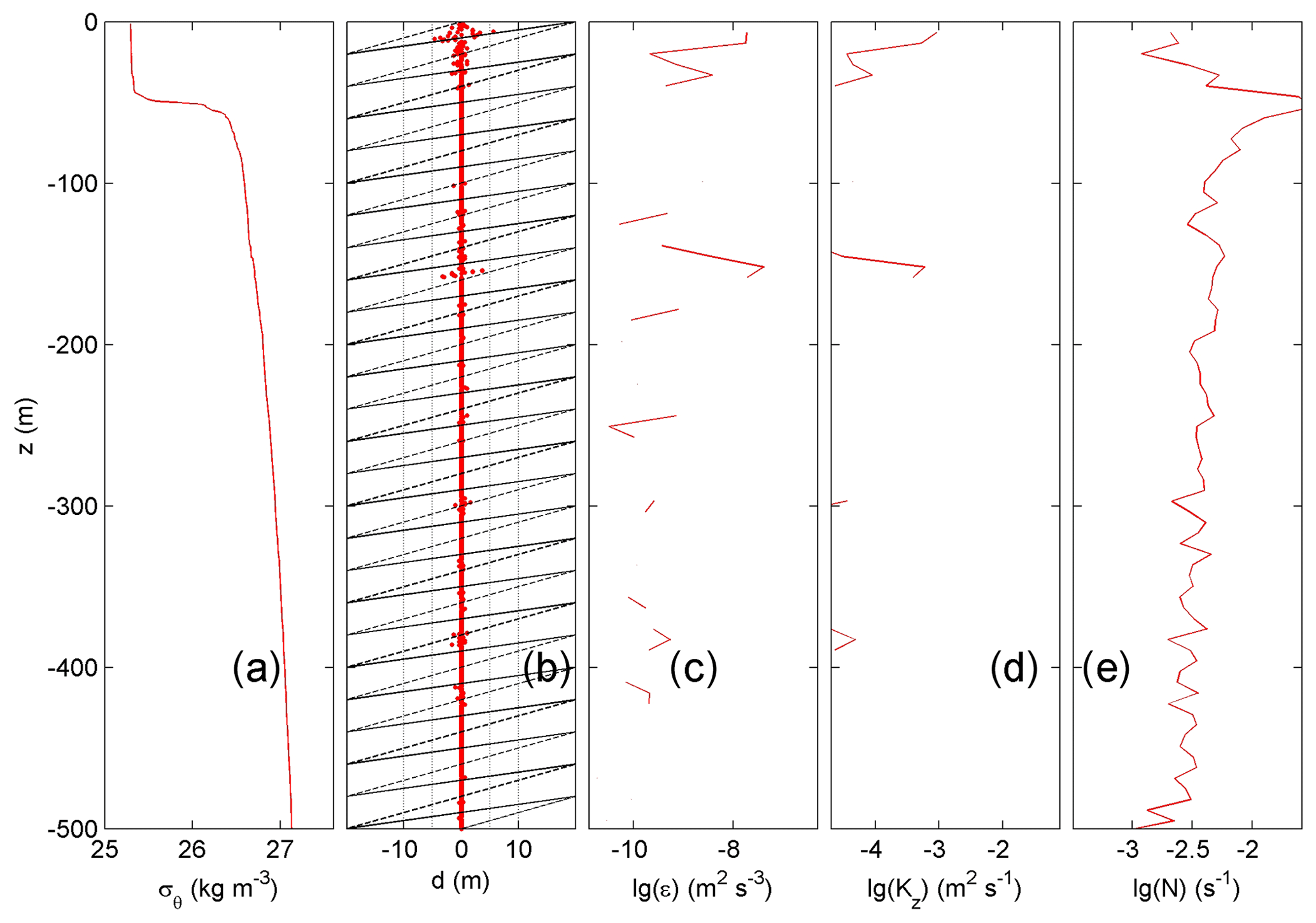
Figure 4 As Fig. 3, but for a southern station. Upper 500 m of turbulence characteristics computed from downcast density anomaly data applying a threshold of 7 × 10⁻⁵ kg m⁻³. Southern station 3, cast 4. (a) Unordered, “raw” profile of density anomaly referenced to the surface. (b) Overturn displacements following reordering of the profiles in (a). Slopes $\mathrm{1}/\mathrm{2}$ (solid lines) and 1 (dashed lines) are indicated. (c) Logarithm of dissipation rate computed from the profiles in (a), rms calculated over 7 m intervals. (d) As (c), but for eddy diffusivity. (e) Logarithm of buoyancy frequency computed after reordering the profiles of (a).

A mid-morning profile at a southern station shows different characteristics (Fig. 4), although 500 m vertically averaged turbulence values are similar to within 10 % of those of the northern station. This 10 % variation is well within the error bounds of about a factor of 2. At this southern station, the near-surface layer is stably stratifying (Fig. 4a) and displays few overturning displacements (Fig. 4b), while the interior demonstrates rarer but occasional intense turbulent overturning (at z = −160 m in Fig. 4), presumably due to internal wave breaking. At greater depths, stratification (∼ N²; Fig. 4e) weakly decreases, together with ε (Fig. 4c) and K_z (Fig. 4d).

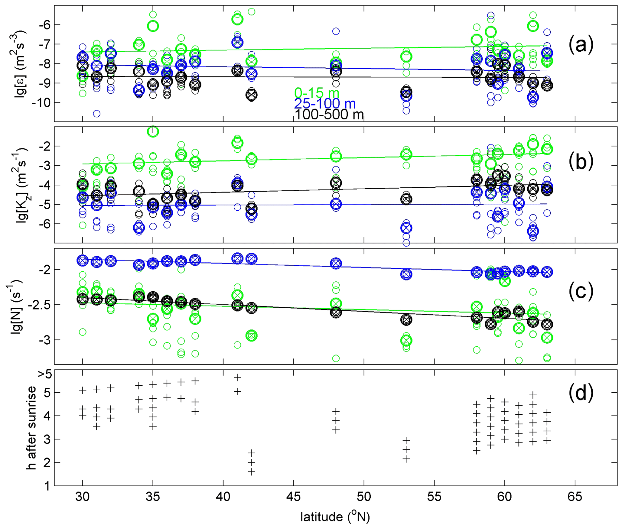
Figure 5 Summer 2017 latitudinal transect along 17 ± 5^∘ W of turbulence values for upper 15 m averages (green) and averages between −100 < z < −25 m (blue, seasonal pycnocline) and −500 < z < −100 m (black, more permanent pycnocline) from short yo-yos of three to six CTD casts. Values are given per cast (o) and station average (heavy circle with x; the size corresponds to ± the standard error for turbulence parameters). (a) Logarithm of dissipation rate. (b) Logarithm of diffusivity. (c) Logarithm of buoyancy frequency (the small symbols have the size of ± the standard error). (d) Hour of sampling after sunrise.

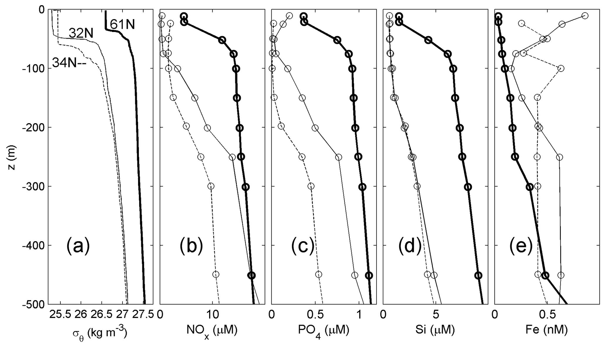
Figure 6 Upper 500 m profiles for stations at three latitudes. (a) Density anomaly referenced to the surface, including profiles from Figs. 3a and 4a. (b) Nitrate plus nitrite. (c) Phosphate. (d) Silicate. (e) Dissolved iron.

Latitudinal overviews are given in Fig. 5 for (1) average values over the upper z > −15 m, which covers the diurnal mainly convective turbulent mixing range from the surface and under the cautionary note that these waters are weakly, but measurably stratified, (2) average values between −100 < z < −25 m, which covers the seasonal strong stratification, and (3) average values between −500 < z < −100 m, which covers the more permanent moderate stratification. Noting that all panels have a vertical axis representing a logarithmic scale, variations over nearly 4 orders of magnitude in turbulence dissipation rate (Fig. 5a) and eddy diffusivity (Fig. 5b) are observed between casts at the same station. This variation in magnitude is typically found in near-surface open-ocean turbulence microstructure profiles (e.g. Oakey, 1982). Still, considerable variability over about 2 orders of magnitude is observed between the averages from the different stations. This variation in station and vertical averages far exceeds the instrumental error bounds of a factor of 2 (0.3 on a log scale) and thus reveals local variability. The turbulence processes occur “intermittently”.

The observed variability over 2 orders of magnitude between yo-yo casts at a single station may be due to active convective overturning during early morning in the near-homogeneous upper layer or due to internal wave breaking and sub-mesoscale variability deeper down. Despite the large variability at stations, trends are visible between stations in the upper 100 m over the 33^∘ latitudinal range going poleward: buoyancy frequency (∼ square root of stratification) steadily decreases significantly (p value  < 0.05) given the spread of values at given stations, with the notion that near-surface (−15 < z < 0 m) values show the same latitudinal trend as deeper down values across a larger spread of values, while turbulence values vary insignificantly with latitude as they remain the same or weakly increase by about 0.5 orders of magnitude (about a factor of 3). At a given depth range, turbulence dissipation rates roughly follow a log-normal distribution with SDs well exceeding 0.5 orders of magnitude. The comparison of latitudinal variations with the (log-normal) distribution is declared insignificant with p > 0.05 when the mean values are found within 2 SDs (see Appendix B). This is not only performed for turbulence dissipation rate but also for other quantities. The trends suggest only marginally larger turbulence going poleward, which is possibly due to larger cooling from above and larger internal wave breaking deeper down. It is noted that the results are somewhat biased by the sampling scheme, which changed from 3 to 4 h after sunrise sampling at high latitudes to 4 to 5 h after sunrise sampling at lower latitudes; see the sampling hours after local sunrise in (Fig. 5d). Its effect is difficult to quantify but should not show up in turbulence values from deeper down (−500 < z < −100 m).

Between −500 < z < −100 m, no clear significant trend with latitude is visible in the turbulence values (Fig. 5a and b), although [K_z] weakly increases with increasing latitude at all levels between −500 < z < 0 m, while buoyancy frequency significantly decreases (Fig. 5c). The data from well-stratified waters deeper down thus show the same latitudinal trend as the observations from the near-surface layers, even though the latter are less well determined because of the weak stratification. Our turbulence values from CTD data also confirm previous results by Jurado et al. (2012), who made microstructure profiler observations from the upper z > −100 m along the same transect. Their results showed turbulence values remain unchanged over 30^∘ latitude or increase by at most 1 order of magnitude, depending on depth level. Their mixed layer (z > ∼ −25 m) turbulence values are similar to our z > −15 m values and 0.5 to 1 order of magnitude larger than the present deeper observations. The slight discrepancy in values averaged over z > −25 m may point to either (i) a low bias due to too strict a criterion of accepting density variations for reordering applied here or (ii) a high bias of the ∼ 10 m largest overturns having similar velocity scales (of about 0.05 m s⁻¹) as their 0.1 m s⁻¹ slowly descending SCAMP (Self Contained Autonomous Microstructure Profiler). At greater depths (−500 < z < −100 m), it is seen in the present observations that the spread in turbulence values over 4 orders of magnitude at a particular station is also large. This spread in values suggests that dominant turbulence processes show similar intermittency in weakly (at high latitudes N ≈ 10^−2.5 s⁻¹) and moderately (at midlatitudes N ≈ 10^−2.2 s⁻¹) stratified waters, respectively, for the given resolution of the instrumentation.

Mean values of N are larger by 0.5 orders of magnitude in the seasonal pycnocline (found in the range −100 < z < −25 m) than those near the surface and in the more permanent stratification below (Fig. 5). Such local vertical variations in N have the same range of variation as observed horizontally across latitudes [30, 63]^∘ per depth level.

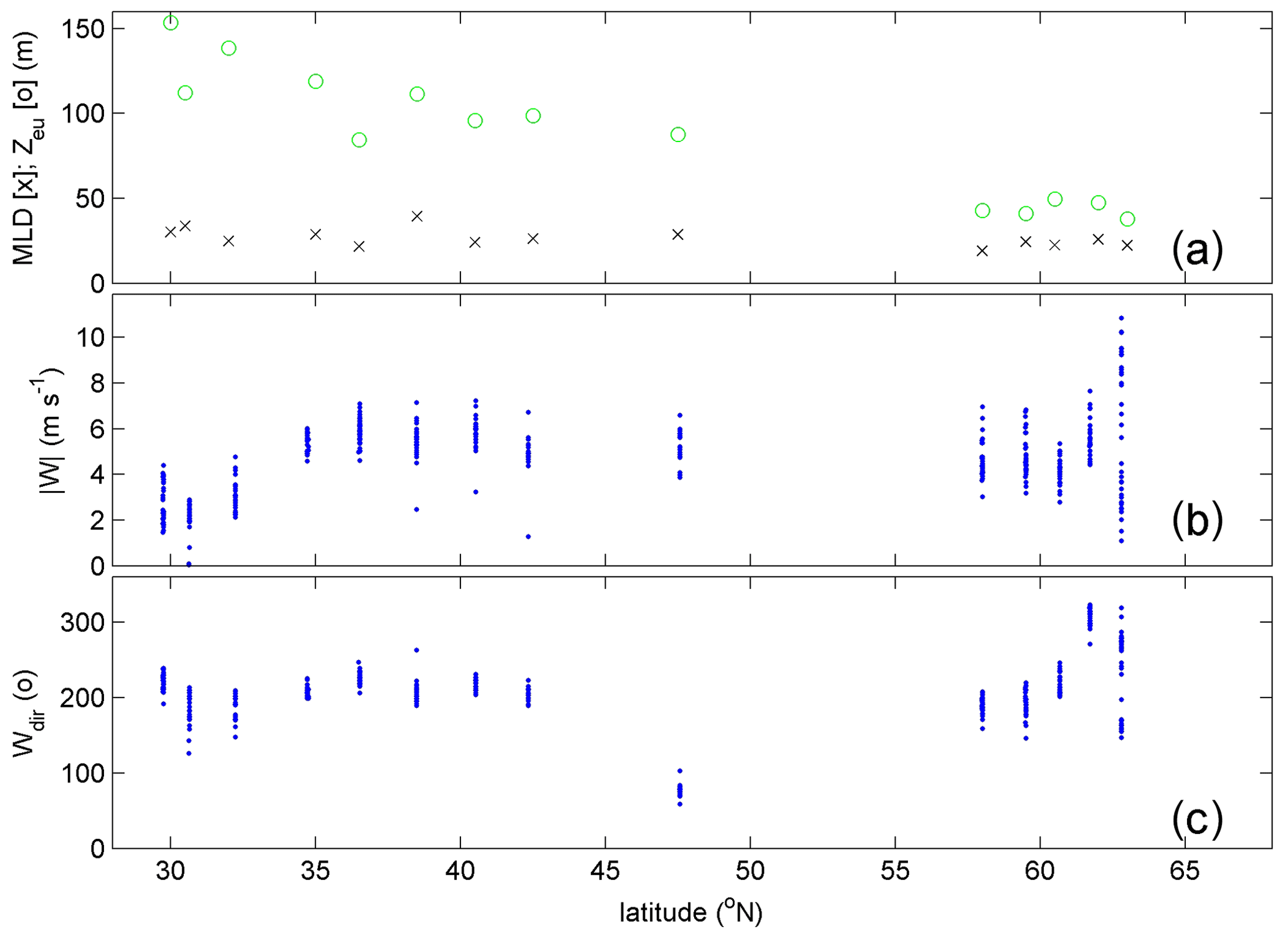
Figure 7 Latitudinal transect of near-surface layers and wind conditions measured at stations during the observational survey. (a) Mixed layer depth (x) and euphotic zone (o). (b) Wind speed. (c) Wind direction.

3.2 Nutrient distributions and fluxes

Vertical profiles of macro-nutrients generally resemble those of density anomaly in the upper z > −500 m (Fig. 6). In the south, low macro-nutrient values are generally distributed over a somewhat larger near-surface mixed layer. The mixed layer depth, at which temperature differed by 0.5 ^∘C from the surface (Jurado et al., 2012), varies between about 20 and 30 m on the southern end of the transect and weakly becomes shallower with latitude (Fig. 7a). This weak trend may be expected from the summertime wind conditions that also barely vary with latitude (Fig. 7b and c). In contrast, the euphotic zone, defined as the depth of the 0.1 % irradiance penetration level (Mojica et al., 2015), demonstrates a clear latitudinal trend decreasing from about 150 to 50 m (Fig. 7a). For z < −100 m below the seasonal stratification, vertical gradients of macro-nutrients are large (Fig. 6b–d). Macro-nutrient values become approximately independent of latitude at depths below z < −500 m. Dissolved iron profiles differ from macro-nutrient profiles, notably in the upper layer near the surface (Fig. 6a). At some southern stations, dissolved iron and to a lesser extent also phosphate have relatively high concentrations closest to the surface. These near-surface concentration increases suggest atmospheric sources, most likely Saharan dust deposition (e.g. Rijkenberg et al., 2012).

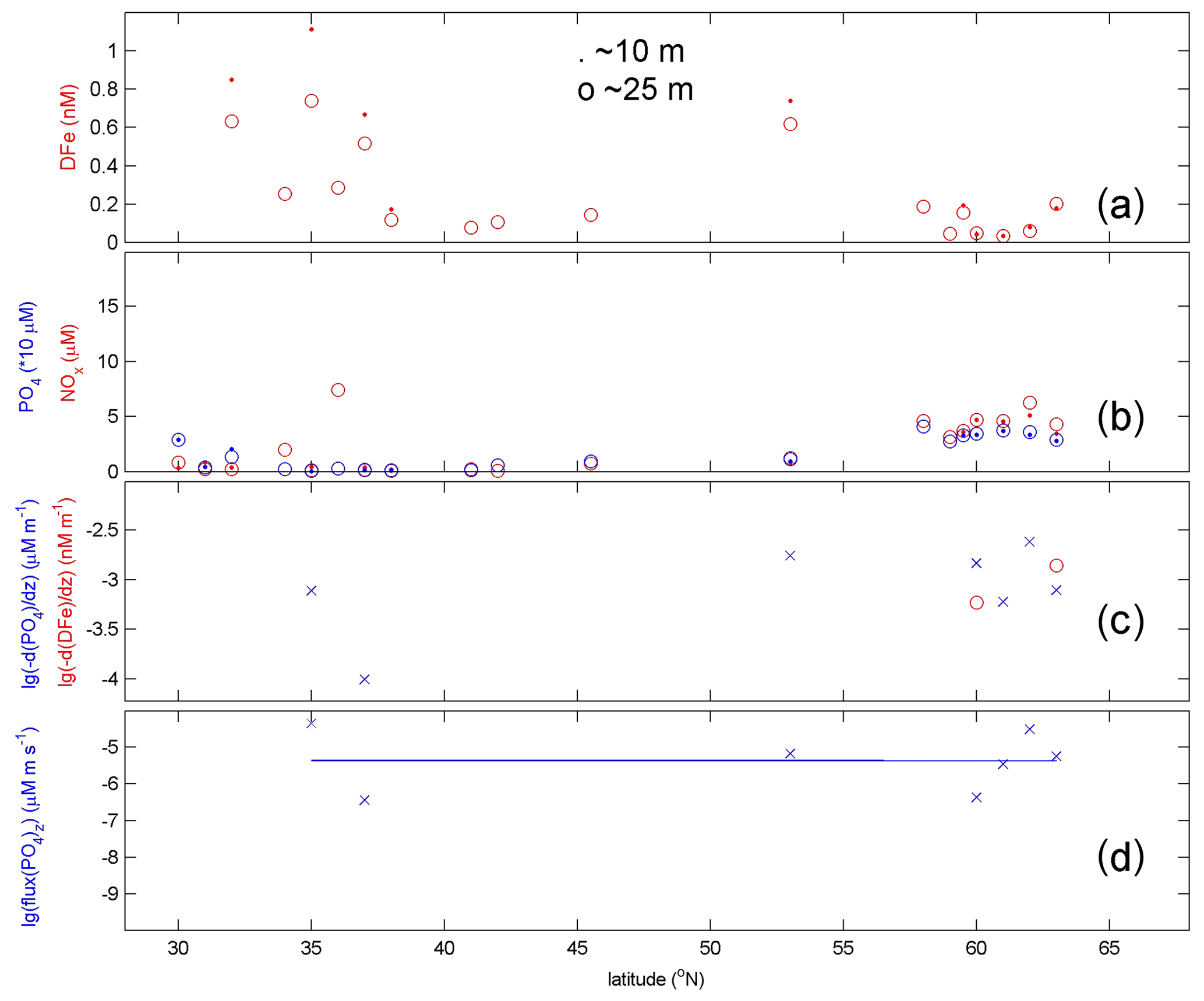
Figure 8 Latitudinal transect of near-surface nutrient concentrations. (a) Dissolved iron measured at depths indicated. Missing values reflect that not all depths were sampled. (b) Nitrate plus nitrite (red) and phosphate (blue, scale times 10) measured at depths indicated in (a). (c) Logarithm of (very weak within SDs of measurements) vertical gradients of dissolved iron in (a) (o, red) and phosphate in (b) (x, blue). Only downgradient values are shown, which excludes several PO₄- and nearly all DFe-gradient values due to near-surface increased values (cf. Fig. 6e, 32^∘ N profile). (d) Upward vertical turbulent fluxes of phosphate concentration gradients in (c). Using average surface K_z from Fig. 5b, valid for depth average (here, ∼ 17 m) of depths in (a).

As a function of latitude in the near-surface mixed layer (Fig. 8), the vertical turbulent fluxes of phosphate (representing the macro-nutrients, for graphical reasons; see the similarity in profiles in Fig. 6b–d) are found to be constant or insignificantly (p > 0.05) increasing (Fig. 8d). Here, the mean eddy diffusivity values for the near-surface layer as presented in Fig. 5 are used for computing the fluxes. It is noted that in this layer turbulent overturning (Figs. 3b and 4b) is larger and nutrients are mainly depleted (Fig. 6), except when replenished from atmospheric sources, in which case gradients reverse sign as in most DFe profiles. Hereby, lateral diffusion is not considered important. Nonetheless, macro-nutrients are seen to increase significantly towards higher latitudes (Fig. 8b). We note that the vertical gradients in Fig. 8c, in which only downgradient values are plotted, are very weak in general within the SD of measurements. The results in Fig. 8d are thus merely indicative, but they are consistent with the results from deeper down presented below.

Figure 9 As Fig. 8, but for −100 < z < −25 m, with fluxes for ∼ 62 m in (d).

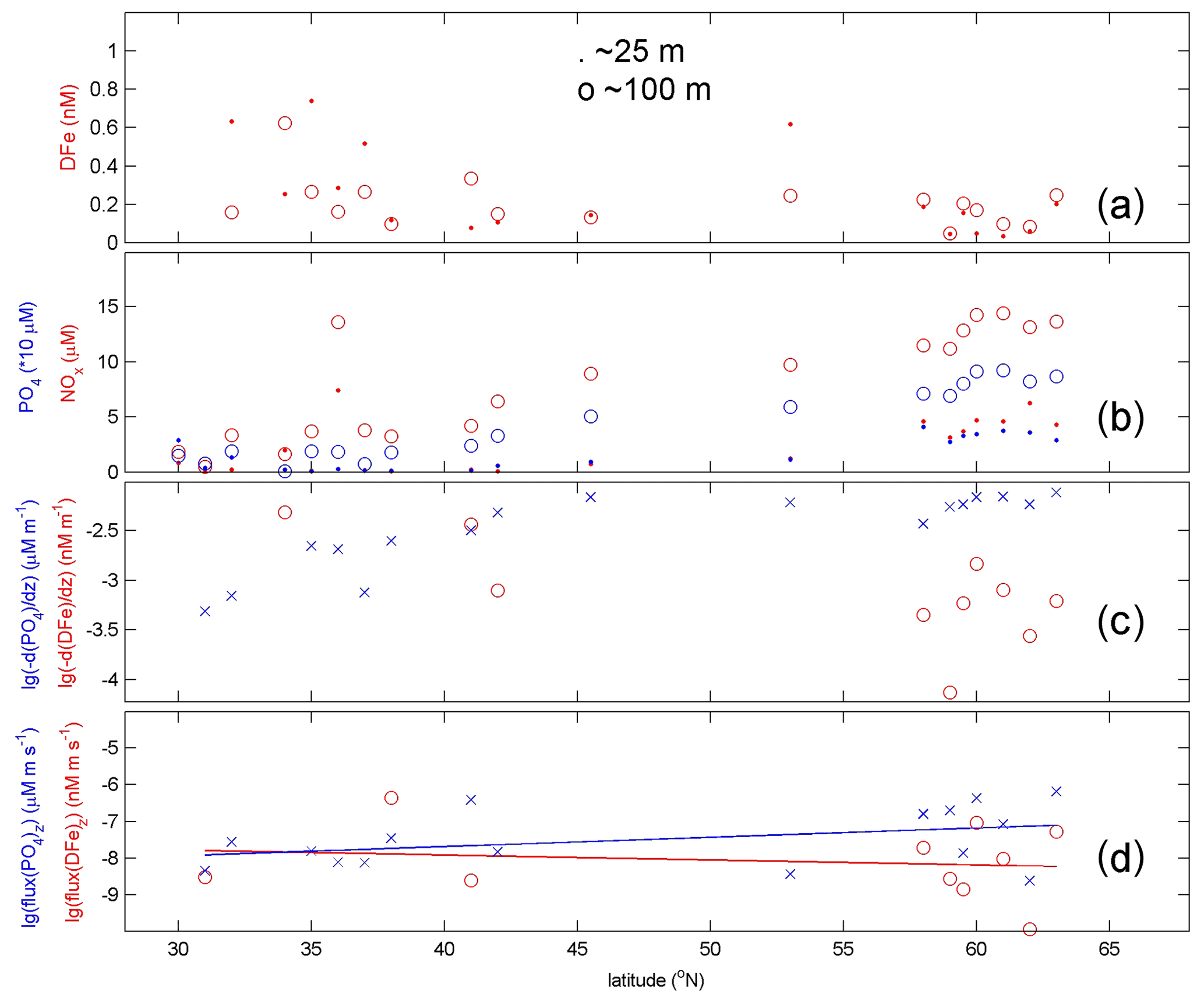
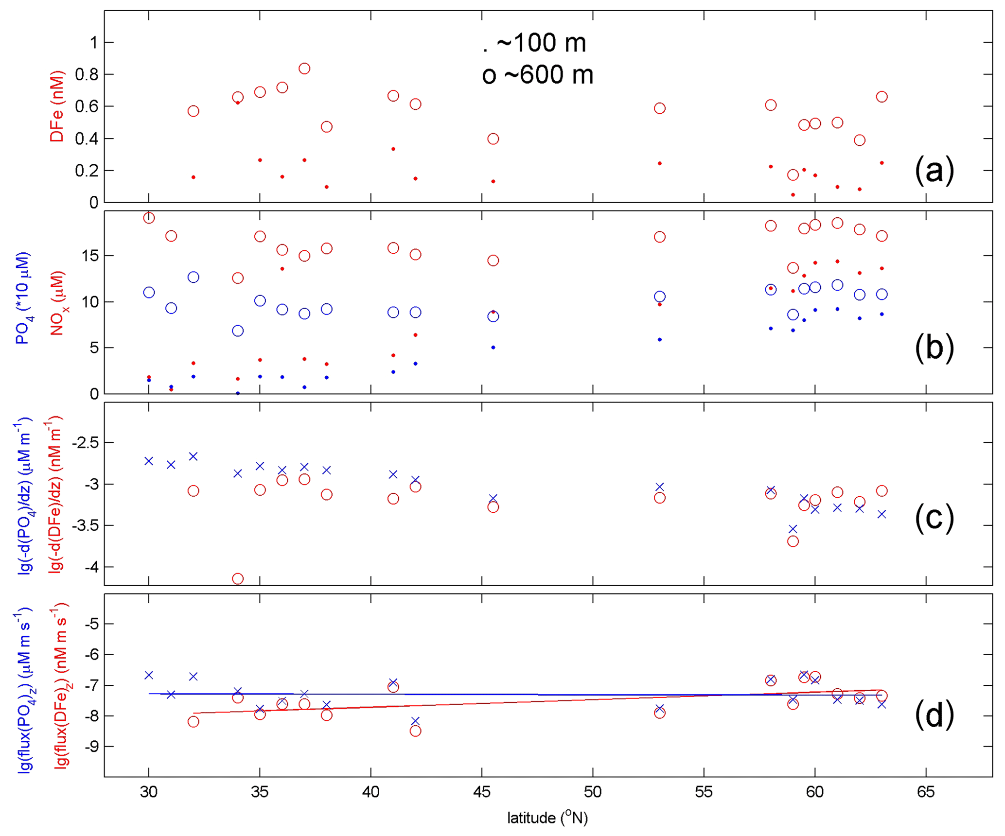
Figure 10 As Fig. 8, but for −600 (few nutrients sampled at 500) < z < −100 m, with fluxes for ∼ 350 m in (d).

More importantly, the significant vertical turbulent fluxes of nutrients across the seasonal pycnocline (Fig. 9) are found ambiguously or statistically independently varying with latitude (Fig. 9d). Likewise, the vertical turbulent fluxes of dissolved iron and phosphate are marginally constant with latitude across the more permanent stratification deeper down (Fig. 10). Nitrate fluxes show the same latitudinal trend, with values around 10⁻⁶ $\mathrm{mmol}{\mathrm{m}}^{-\mathrm{2}}{\mathrm{s}}^{-\mathrm{1}}$. Overall, the vertical turbulent nutrient fluxes across the seasonal and more permanent stratification resemble those of the physical vertical turbulent mass flux, which is equivalent to the distribution of turbulence dissipation rate and which is latitude invariant (Fig. 5a).

4 Discussion

Practically, the upright positioning of the CTD instrument while using an adaptation consisting of a custom-made equal-surface inlet worked well to minimize ship-motion effects on variable flow-imposed temperature variations. This improved calculated turbulence values from CTD observations in general and in near-homogeneous layers in particular. The indirect comparison with turbulence values determined from previous microstructure profiler observations along the same transect (Jurado et al., 2012) confirms the same trends, although occasionally turbulence values were lower (to 1 order of magnitude in the present study). This difference in values may be due to the time lapse of 8 years between the observations, but more likely it is due to inaccuracies in one or both methods. It is noted that any ocean turbulence observations cannot be made better than to within a factor of 2 (Neil Oakey, personal communication, 1991). In that respect, the standard CTD instrument with the adaptation presented here is a cheaper solution than additional microstructure profiler observations. Although the general understanding, mainly amongst modellers, is that the Thorpe length method overestimates diffusivity (e.g. Scotti, 2015; Mater et al., 2015), this view is not shared amongst ocean observers (e.g. Gregg et al., 2018). In the large parameter space of the high Reynolds number environment of the ocean, turbulence properties vary constantly, with an intermingling of convection and shear-induced turbulence at various levels. Given sufficient averaging and adequate mean value parametrization, the Thorpe length method is not observed to overestimate diffusivity. This property of adequate and sufficient averaging yields similar mean parameter values in recent modelling results estimating a mixing coefficient near the classical bound of 0.2 in stationary flows for a wide range of conditions (Portwood et al., 2019). It is noted that diffusivity always requires knowledge of stratification to obtain a turbulent flux, and it is better to consider turbulence dissipation rate for intercomparison purposes. Nevertheless, future research may perform a more extensive comparison between Thorpe-scale analysis data and deeper microstructure profiler data.

While our turbulence values are roughly similar to those of others transecting the NE Atlantic over the entire water depth (Walter et al., 2005; Kunze et al., 2006), the focus in the present paper is on the upper 500 m because of its importance for upper-ocean marine biology. Our study demonstrates a significant decrease in stratification with increasing latitude and decreasing temperature that, however, does not lead to significant variation in turbulence values and vertical turbulent fluxes. Our direct estimates of the turbulent flux of nitrate into the euphotic zone are 1 to 2 orders of magnitude less than the previously estimated rate of nitrate uptake for the summer period. Our turbulent flux of nitrate values are of the same order of magnitude as reported by others (Cyr et al., 2015, and references therein). In particular, the Martin et al. (2010) study in the northeast Atlantic Ocean (at 49^∘ N, 16^∘ W) reported similar vertical nutrient fluxes during summer, which provides confidence in the methods used. The same authors reported that the vertical nitrate flux into the euphotic zone was much lower than the rate of nitrate update at the time. To determine these nitrate uptake rates, they spiked water samples with a minimum of 0.5 µM nitrate, representing ∼ 10 % of the ambient nitrate concentration. In our study area, the ambient nitrate concentrations in the euphotic zone were much lower (see also Mojica et al., 2015), implying a higher relative importance of nitrate input to the overall uptake demand. Still, primary productivity in the oligotrophic euphotic zone, as well as in the high-latitude Atlantic, is mainly fuelled by recycling (e.g. Gaul et al., 1999; Achterberg et al., 2020), and the supply of new nutrients by turbulent fluxes, however small, provides a welcome addition. Besides nutrient input resulting from vertical turbulent fluxes, there is a role for latitudinal differences through the supply of nutrients by deep mixing events and, depending on the location, also potential upwelling and lateral transport events.

We suggest that internal waves may drive the feedback mechanism, participating in the subtle balance between destabilizing shear and stable (re)stratification. Molecular diffusivity of heat is about 10⁻⁷ m² s⁻¹ in seawater and nearly always smaller than turbulent diffusivity in the ocean. The average values of K_z during our study were typically 100 to 1000 times larger than molecular diffusivity, which implies that turbulent diapycnal mixing drives vertical fluxes despite the relatively slow turbulence compared to surface wave breaking. Depending on the gradient of a substance like nutrients or matter, the relatively slow turbulence may not necessarily provide weak fluxes $-K_z\mathrm{d}\left(\text{substance}\right)/\mathrm{d}z$ into the photic zone. In the central North Sea, a relatively low mean value of K_z = 2 × 10⁻⁵ m² s⁻¹, comparable to values over the seasonal pycnocline here, was found sufficient to supply nutrients across the strong summer pycnocline to sustain the entire late-summer phytoplankton bloom in near-surface waters and to warm up the near-bottom waters by some 3 ^∘C over the period of seasonal stratification (van Haren et al., 1999). There, the turbulent exchange was driven by a combination of tidal currents modified by the stratification and shear by inertial motions driven by the Coriolis force (inertial shear) and internal wave breaking. Such drivers are also known to occur in the open ocean, although to an unknown extent.

The here observed (lack of) latitudinal trends of ε, K_z, and N yield approximately the same information as the vertical trends in these parameters at all stations. In the vertical for z < −200 m, turbulence values of ε and K_z weakly vary with stratification. This is perhaps unexpected and contrary to the common belief of stratification hampering vertical turbulent exchange of matter including nutrients. It is less surprising when considering that increasing stratification is able to support larger shear. Known sources of destabilizing shear include near-inertial internal waves of which the vertical length scale is relatively small compared to other internal waves, including internal tides (LeBlond and Mysak, 1978).

The dominance of inertial shear over shear by internal tidal motions (internal tide shear), together with larger energy in the internal tidal waves, has been observed in the open ocean, e.g. in the Irminger Sea around 60^∘ N (van Haren, 2007). The frequent atmospheric disturbances in that area generate inertial motions and dominant inertial shear. Internal tides have larger amplitudes, but due to much larger length scales they generate weaker shear than inertial motions. Small-scale internal waves near the buoyancy frequency are abundant and may break sparsely in the ocean interior outside regions of topographic influence. However, larger destabilizing shear requires larger stable stratification to attain a subtle balance of “constant” marginal stability (van Haren et al., 1999). Not only storms but all geostrophic adjustments, such as frontal collapse, may generate inertial wave shear also at low latitudes (Alford and Gregg, 2001), so that overall latitudinal dependence may be negligible. If shear-induced turbulence in the upper ocean is dominant, it may thus be latitudinally independent (shallow observations by Jurado et al., 2012; deeper observations in present study). There are no indications that the overall open-ocean internal wave field and (sub-)mesoscale activities are energetically very different across the midlatitudes. If internal tide sources had dominated our observations, clear differences in turbulence dissipation rates would have been found at our station near 48^∘ N (near the Porcupine Bank), for example, compared with those at other stations.

Summarizing, our study infers that vertical nutrient fluxes did not vary significantly with latitude and stratification. This suggests that predicted changes in the physical environment due to global ocean warming have little effect on vertical turbulent exchange. Supposing that enhanced warming leads to more stable stratification, more internal waves can be supported (LeBlond and Mysak, 1978), which upon breaking can maintain the extent of vertical turbulent exchange and thereby, for example, vertical nutrient fluxes. We thus hypothesize that, from a physical environment perspective, in stratified oligotrophic waters the nutrient input from deeper waters and corresponding summer phytoplankton productivity and growth are not expected to change (much) with future global warming. We invite future observations and numerical modelling to further investigate this suggestion and associated feedback mechanisms such as internal wave breaking.

Appendix A: Modification of CTD pump tubing to minimize hydrodynamic ram effects

The unique pump system on SeaBird Electronics (SBE) CTD instruments, foremost on their high-precision full ocean depth shipborne and cable-lowered SBE911, minimizes the effects of flow variations (and inversions) past its T–C sensors (SeaBird, 2012). This reduction in flow variation is important because the T sensor has a slower response than the C sensor. As data from the latter are highly temperature dependent, besides being pressure dependent, the precise matching of all three sensors is crucial for establishing proper salinity and density measurements, especially across rapid changes in any of the parameters. As flow past the T sensor causes higher measurement values due to friction at the sensor tip, flow fluctuations are to be avoided as they create artificial T variations of about 1 mK s m⁻¹ (Larson and Pedersen, 1996).

However, while the pump itself is one thing, its tubing needs careful mounting as well, with the in- and outlet at the same depth level (Sea-Bird, 2012). This is to prevent ram pressure P = ρU², for density ρ and flow speed U. Unfortunately, the SBE manual shows tubing of different diameters, for in- and outlet. Different diameter tubing leads to velocity fluctuations of ± 0.5 m s⁻¹ past the T sensor, as was concluded from a simple experiment by van Haren and Laan (2016). The flow speed variations induce temperature variations of ± 0.5 mK and are mainly detectable in weakly stratified waters such as in the deep ocean but also near the surface as observed in the present data. Using tubes of the same diameter opening counteracted most of the effect, but only if the surface of the tube opening is perpendicular to the main CT motion as in a vertically mounted CTD instrument. If it is parallel to the main motion as in a horizontally mounted CTD instrument, the effect was found to be adverse. The make-shift onboard experiment in van Haren and Laan (2016) has now been cast into a better design (Fig. A1), of which the first results are presented in this paper.

Figure A1 SBE911 CTD pump in- and outlet modification following the findings in van Haren and Laan (2016). (a) The T and C sensors clamped together with a structure holding in- and outlet pump tubing of exactly the same diameter, separated at 0.3 m distance in the horizontal plane. (b) The modification of (a) mounted in the CTD frame.

Appendix B: PDFs of vertically averaged dissipation rate in comparison with latitudinal trends

Ocean turbulence dissipation rate generally tends to a nearly log-normal distribution (e.g. Pearson and Fox-Kemper, 2018), so that the probability density function (PDF) of the logarithm of ε values is normally distributed and can be described by the first two moments, the mean, and its SD. It is seen in Fig. B1 that the overall distribution of all present data indeed approaches log-normality, despite the relatively large length scale used in the computations (cf. Yamazaki and Lueck, 1990). When the data are split into the three depth levels as in Fig. 5a, it is seen that ε in the upper z > −15 m layer is not log-normally distributed due to a few outlying high values confirming an ocean state dominated by a few turbulence bursts (Moum and Rippeth, 2009), whereas ε in the deeper more stratified layers is nearly log-normally distributed.

When we compare the mean and SDs of the distributions with the extreme values of the latitudinal trends as computed for Fig. 5a it is seen that the extreme values are not found outside 1 SD from the mean value for any of the three depth levels. In fact, for deeper stratified waters the extreme values of the trends are found very close to the mean value. It is concluded that the mean dissipation rate does not show a significant trend with latitude, at all depth levels. The same exercise yields extreme buoyancy frequency values lying outside 1 SD from the mean values for well-stratified waters, from which we conclude that stratification significantly decreases with latitude. This is inferable from Fig. 5c by investigating the spread of mean values around the trend line.

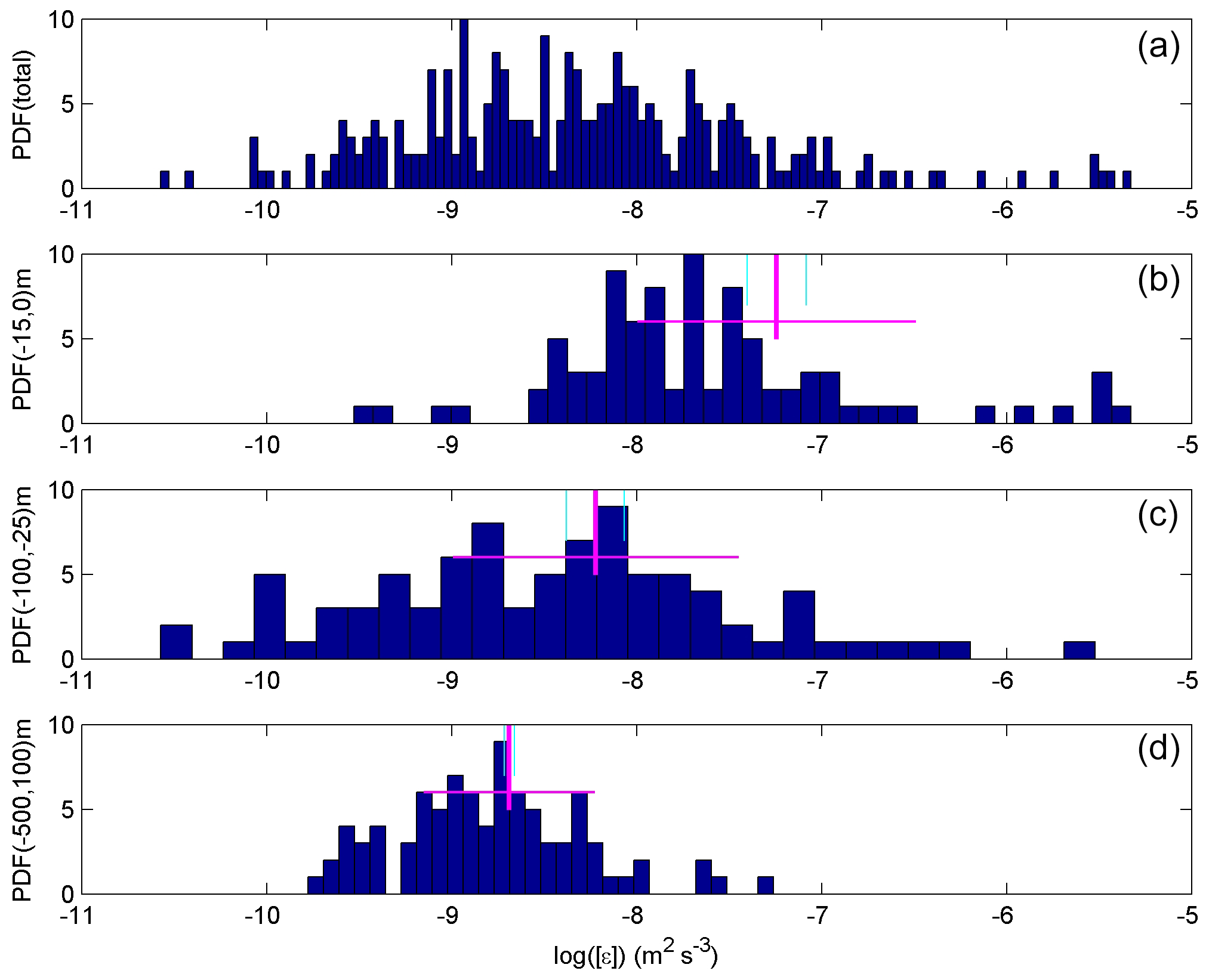
Figure B1 Probability density functions of logarithm of the vertically averaged dissipation rate in comparison with latitudinal trend extreme values. (a) Distribution as a function of latitude for all data. (b) As (a), but for the upper 15 m averages only. The mean value is given by the vertical purple line, with the horizontal line indicating  ± 1 SD. The vertical light-blue lines indicate the best-fit value of the trend for 30 and 63^∘ N. (c) As (b), but for averages between −100 < z < −25 m. (d) As (c), but for averages between −500 < z < −100 m.