Seasonal variability of the Atlantic Meridional Overturning Circulation at 11° S inferred from bottom pressure measurements

Bottom pressure observations on both sides of the Atlantic basin, combined with satellite measurements of sea level anomalies and wind stress data, are utilized to estimate variations of the Atlantic Meridional Overturning Circulation (AMOC) at 11^∘ S. Over the period 2013–2018, the AMOC and its components are dominated by seasonal variability, with peak-to-peak amplitudes of 12 Sv for the upper-ocean geostrophic transport, 7 Sv for the Ekman and 14 Sv for the AMOC transport. The characteristics of the observed seasonal cycles of the AMOC and its components are compared to results from an ocean general circulation model, which is known to reproduce the variability of the Western Boundary Current on longer timescales. The observed seasonal variability of zonally integrated geostrophic velocity in the upper 300 m is controlled by pressure variations at the eastern boundary, while at 500 m depth contributions from the western and eastern boundaries are similar. The model tends to underestimate the seasonal pressure variability at 300 and 500 m depth, especially at the western boundary, which translates into the estimate of the upper-ocean geostrophic transport. In the model, seasonal AMOC variability at 11^∘ S is governed, besides the Ekman transport, by the geostrophic transport variability in the eastern basin. The geostrophic contribution of the western basin to the seasonal cycle of the AMOC is instead comparably weak, as transport variability in the western basin interior related to local wind curl forcing is mainly compensated by the Western Boundary Current. Our analyses indicate that while some of the uncertainties of our estimates result from the technical aspects of the observational strategy or processes not being properly represented in the model, uncertainties in the wind forcing are particularly relevant for the resulting uncertainties of AMOC estimates at 11^∘ S.

1 Introduction

The Atlantic Meridional Overturning Circulation (AMOC) plays a major role in the global oceanic heat budget. About 88 % of the maximum heat transport in the subtropical North Atlantic (1.3 PW; e.g. Lavin et al., 1998) is carried by the AMOC (Johns et al., 2011). Because of the AMOC, there is substantial northward heat transport across the Atlantic Equator (e.g. Talley, 2003), which is unique among global oceans. Simplifying the circulation in the Atlantic to a two-dimensional latitude–depth plane, the AMOC connects warm waters flowing northward in the upper ocean and cold waters flowing southward at depth across all latitudes through water mass transformation, for example, in the subpolar North Atlantic or near the Southern Ocean (e.g. Buckley and Marshall, 2016). With the AMOC representing the strongest mode of northward heat transport by the ocean, it is essential to provide the observational evidence of the mechanisms that control its structure and variability in order to understand the present-day climate, validate climate simulations and improve predictions. Historically, the strength and structure of the AMOC were estimated based on shipboard hydrographic sections establishing the mean AMOC strength and related heat transport (e.g. Richardson, 2008). The first trans-basin mooring array – the Rapid Climate Change – Meridional Overturning Circulation and Heatflux Array (RAPID/MOCHA) transport array at 26^∘ N – has continuously measured the temporal variability of the AMOC since the early 2000s (Hirschi et al., 2003). Those observations showed that large AMOC variations can occur on a range of timescales – from weeks to decades (e.g. Srokosz and Bryden, 2015). Kanzow et al. (2007) showed that not only the Ekman but even more so the geostrophic contribution to the AMOC exhibit pronounced high-frequency variability with periods up to few weeks. Kanzow et al. (2010) demonstrated that the strong seasonal cycle in the AMOC strength at 26^∘ N leads to aliasing, when estimating the AMOC strength from single hydrographic sections. They also found the upper-ocean geostrophic AMOC contribution to dominate on seasonal timescales, while Chidichimo et al. (2010) discovered those to be primarily driven by processes at the eastern boundary.

Today, there are several ongoing international efforts monitoring the AMOC at selected latitudes (e.g. Frajka-Williams et al., 2019), such as the OSNAP array in the subpolar North Atlantic (since 2014; Lozier et al., 2019), the RAPID array in the subtropical North Atlantic at 26^∘ N (since 2004; Cunningham et al., 2007; McCarthy et al., 2015), the MOVE array in the tropical North Atlantic at 16^∘ N (since 2001; Kanzow et al., 2008; Send et al., 2011; Frajka-Williams et al., 2018), the SAMBA array in the subtropical South Atlantic at 34.5^∘ S (since 2009; Meinen et al., 2018), as well as other programmes measuring important components of the overturning, such as the Western Boundary Current (WBC) arrays at 53^∘ N (since 1997; Zantopp et al., 2017), at 39^∘ N (line W; 2004–2014; Toole et al., 2017) and at 11^∘ S (2000–2004 and since 2013; Hummels et al., 2015), the array across the North Atlantic Current at 47^∘ N (NOAC array; Roessler et al., 2015), the deep overflow observations through Denmark Strait (Jochumsen et al., 2017) or Faroe Bank Channel (Hansen et al., 2016). In this study, we will present the first estimate of basin-wide AMOC variations in the tropical South Atlantic from the TRACOS (Tropical Atlantic Circulation and Overturning at 11^∘ S) array.

The western tropical South Atlantic constitutes a key region for the exchange of water masses, heat and salt between the Southern Hemisphere and Northern Hemisphere (Biastoch et al., 2008b; Schmidtko and Johnson, 2012; Kolodziejczyk et al.,2014; Hummels et al., 2015; Lübbecke et al., 2015; Herrford et al., 2017). Several observational and modelling studies (e.g. Rühs et al., 2015; Zhang et al., 2011) suggest that 11^∘ S is a good place to monitor water mass signal propagation, changes in the WBC transport and, with that, changes in the AMOC transport. At 11^∘ S the WBC regime is comprised of the northward North Brazil Undercurrent (NBUC) with a subsurface velocity maximum at about 200 m and the southward Deep Western Boundary Current (DWBC) below 1200 m (e.g. Schott et al., 2005). The NBUC is known to originate from the southern branch of the South Equatorial Current (da Silveira et al., 1994), which transports subtropical waters towards Brazil and bifurcates between 14 and 28^∘ S (Stramma and England, 1999; Boebel et al., 1999; Wienders et al., 2000). From 2000 to 2004, a first mooring array was deployed at 11^∘ S to observe the variability of the WBC and its components – the NBUC and the DWBC below. Schott et al. (2005) found the NBUC to carry 25 Sv northward on average. The NBUC showed a strong seasonal cycle, which seems to be out of phase with the seasonal variations in the DWBC. Intraseasonal signals could also be observed: Dengler et al. (2004) described a spectral peak in the velocity time series at a period of 60–70 d, which was observed in most of the moored records but was strongest within the DWBC. They concluded that the DWBC transport at 11^∘ S is mainly accomplished by migrating eddies. Further, Veleda et al. (2011) could relate variability at periods of 2–3 weeks to coastal trapped waves (CTWs) propagating from 22 to 36^∘ S equatorward along the Brazilian coast. In July 2013, a similar mooring array was again deployed at 11^∘ S (Hummels et al., 2015) and is still in place. Comparing the two observational periods, Hummels et al. (2015) did not find significant changes in the averaged NBUC and DWBC transport. Furthermore, they could show that the interannual NBUC variability observed between 2000 and 2004 is consistent with the output of a forced ocean general circulation model (OGCM) named INALT01. Decadal variability in INALT01 was also found to be similar to transport estimates based on historical hydrographic observations from Zhang et al. (2011). To date, Zhang et al. (2011) provide the only NBUC time series derived from hydrographic observations spanning several decades. They estimated multi-decadal variability of the NBUC to be of similar order to its seasonal cycle and, because of the connection to the Atlantic Multidecadal Variability, suggested the NBUC to serve as an index for AMOC variations on these timescales. In a model study, Rühs et al. (2016) found decadal to multi-decadal buoyancy-forced changes in the AMOC transport to manifest themselves in NBUC transport (at 6^∘ S); however, these changes are also masked by interannual wind-driven variability.

With the resumption of the mooring array at 11^∘ S in 2013, the observational programme was also extended by installing a mooring array for direct velocity measurements across the continental slope off Angola. Studies based on these observations showed that the circulation there is weak and dominated by seasonal variability associated with remotely forced waves (Kopte et al., 2017, 2018). As shown in several model studies, most of the intraseasonal (T>120 d) to interannual variability in that region is induced by a wave response to equatorial wind forcing that generates equatorial Kelvin waves propagating eastward and, while reaching the eastern boundary, transferring a part of their energy as CTWs further to the south towards 11^∘ S (Illig et al., 2004, 2018; Bachèlery et al., 2016; Imbol Koungue et al., 2017).

Besides the moored observations at 11^∘ S, PIESs (pressure-inverted echo sounders) or single bottom pressure recorders (BPRs) were deployed on both sides of the Atlantic. Within some of the other programmes targeting AMOC fluctuations – such as RAPID (Kanzow et al., 2010; Meinen et al., 2013; McCarthy et al., 2015), MOVE (Kanzow et al., 2006, 2008) and SAMBA (Meinen et al., 2018; Kersalè et al., 2020) – bottom pressure (BP) measurements are used to estimate the time-varying portion of a barotropic reference velocity which is then combined with the internal geostrophic velocity derived from differences in dynamic height derived from full-depth dynamic height moorings or the PIES travel times. But, circulation changes in z coordinates can also be estimated using only a series of bottom pressure measurements installed at different depths on the western and eastern continental slopes. In a model study, Bingham and Hughes (2008) showed that this works well down to around 3000 m, even with only western boundary measurements. In our study, we use the BP differences across the basin at 300 and 500 m depth to estimate the geostrophic contribution to AMOC variations in the tropical South Atlantic over the period 2013–2018 and investigate its seasonal variability.

2 Observational data

2.1 Bottom pressure time series

Over the period 2013–2018, five BPRs were deployed at 11^∘ S (Table 1). In May 2013, together with the WBC mooring array, two bottom-mounted PIESs were installed across the Brazilian continental slope at 300 and 500 m depth. PIESs measure the acoustic travel time to the surface, as well as bottom pressure. In this study, we only used the BP time series. Then, 1 year later, another set of PIESs was deployed at the same locations. While of the first set only the 500 m sensor could be recovered, the second set was maintained in September 2016 and spring 2018. Note that the two PIESs at 500 m, KPO 1109 and KPO 1135 (Table 1), were located only ∼1 km away from each other over the period May 2014–October 2015. At the eastern boundary off Angola, two SBE 26plus sensors (single or attached to an acoustic Doppler current profiler (ADCP) shield) measured pressure at 300 and 500 m depth from July 2013 to November 2015. The instruments were re-deployed but could not be recovered again. We assume that they were lost due to extensive fishing in the region.

Table 1 Collection of available BP measurements at 11^∘ S. Acronyms used throughout this article are given in the first column; official mooring IDs and instrument types are listed in the second and third columns. Columns 4–6 give the positions, depths and deployment periods for each BP measurement. The BP data can be found at https://doi.org/10.1594/PANGAEA.907589.

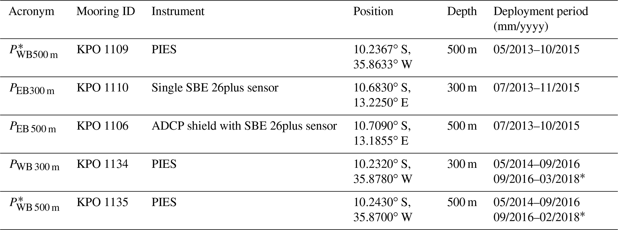
^* These sensors were re-deployed in 2018 and are currently in place.

For our analyses, the available BP records were de-spiked, interpolated from an original sampling rate of 10 min to hourly values and de-tided using harmonic fits with tidal periods shorter than 35 d. All tidal harmonics were calculated by performing a classical harmonic analysis (Codiga, 2011). The tidal models for T<35 d capture between 97.0 % and 99.6 % of the total variance in the original BP time series. After removing these higher-frequency tides, the remaining variance is mainly related to seasonal variations and low-frequency instrument drifts. Instrument drifts vary substantially between the five instruments: while KPO 1106 shows almost no drift, all other sensors exhibit a combination of exponential and linear behaviour but with different signs and at different rates (Fig. 1a). Unfortunately, we were not able to directly relate individual drift behaviour to pressure effects or material creep. Earlier studies (e.g. Watts and Kontoyiannis, 1990; Johns et al., 2005; Kanzow et al., 2006; Cunningham, 2009) found that subtracting a least-squares exponential–linear fit of the form $P_{\mathrm{Drift}}\left(t\right)=a\left[\mathrm{1}-e^{-bt}\right]+ct+d$ from the pressure time series to be the procedure that works best for the PIES. As the SBE26plus recorders were also equipped with quartz pressure sensors, we decided to “de-drift” all five sensors similarly by subtracting exponential–linear fits as described above. Kanzow et al. (2006) also discussed the problem of this empirical de-drifting being unable to distinguish between the instrumental drift and ocean signals of the order of or longer than the time series. This means that, for example, seasonal signals can leak into the fit and its removal from the time series can reduce seasonal signals in return. We attempted to solve this problem by iteratively fitting an exponential–linear drift as well as annual and semi-annual harmonics. The first guess of the exponential–linear drift was removed from the original time series, and annual and semi-annual harmonics were fitted to the de-drifted time series. This first guess was iteratively improved by calculating new exponential–linear fits after subtracting the iteratively improved annual and semi-annual harmonics from the original data. After three repetitions, the fits tended to converge. Both fits from the third repetition are shown in Fig. 1a. For further analyses, we removed the derived instrument drift from the original BP time series and averaged to daily values (Fig. 1b).

Figure 1 Bottom pressure (BP) anomalies measured at 11^∘ S off Angola at 300 (pink) and 500 m (red), as well as off Brazil at 300 (light blue) and 500 m (blue) depth. (a) Instrument drifts that are removed from, as well as the sum of the drift and the combined annual and semi-annual harmonics fitted to, the individual BP anomaly time series. (b) Daily time series of BP anomalies after de-tiding and de-drifting (see text for details).

2.2 Sea level anomalies

To estimate pressure variability at the surface, we used sea level anomalies (SLAs) from the delayed-time “all-sat-merged” data set of global sea surface height, produced by Ssalto/Duacs and provided by the Copernicus Marine Environment Monitoring Service (CMEMS). The multi-satellite altimeter sea surface heights are mapped on a $\mathrm{0.25}{}^{\circ }\times \mathrm{0.25}{}^{\circ }$ grid (e.g. Pujol et al., 2016) and are available for the period 1993–2018 at daily resolution. To obtain pressure variation near the boundaries, SLA grid points were chosen closest to the Brazilian and Angolan coasts at 11^∘ S, respectively. The sensitivity of our results to SLA changes with distance to the coast (Fig. 2c, d) was tested: at the western boundary, off Brazil, the phase of the annual harmonic slightly changes with distance to the coast – about 30 d over 0.5^∘ longitude. At the eastern boundary, off Angola, the phases of both annual and semi-annual harmonics are constant over the distance between the location of the 300 m BPR and the coast.

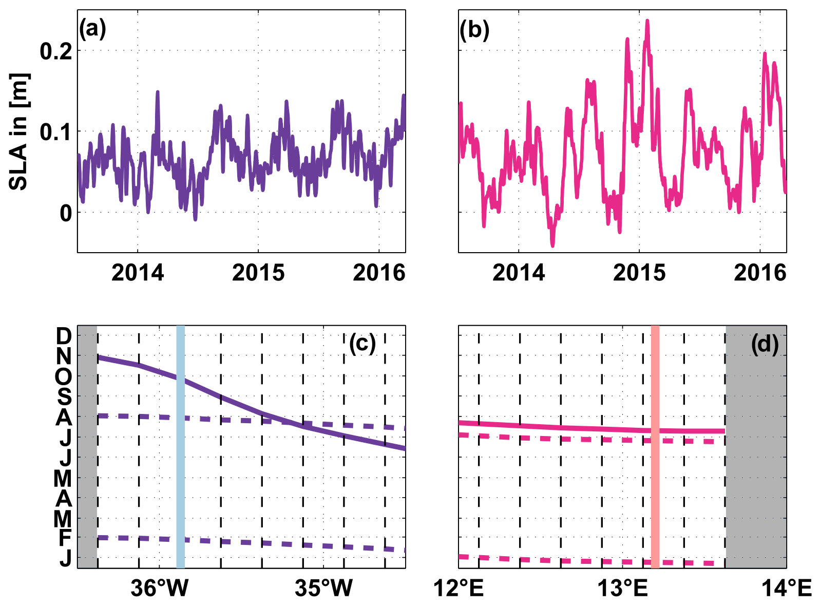
Figure 2 Time series of SLA over the period 2013–2018 – chosen close to the western (purple; a) and eastern boundaries (magenta; b). Phases of the minima of the annual (solid curve) and semi-annual (dashed curves) harmonics as a function of longitude near the western (c) and eastern (d) boundaries. In panels (c–d), the dashed black lines represent the zonal grid spacing of the SLA data and grey areas mark land. Light blue (c) and pink (d) lines mark the locations of the 300 m BPRs at the western (c) and eastern (d) boundaries.

2.3 Wind stress

In order to estimate the Ekman contribution to AMOC variability at 11^∘ S, we used gridded daily wind stress fields from MetOp/Advanced Scatterometer (ASCAT) retrievals. Those are available for the period 2007–2018 and with a spatial resolution of $\mathrm{0.25}{}^{\circ }\times \mathrm{0.25}{}^{\circ }$ (Bentamy and Croizé-Fillon, 2012). The near-surface Ekman transport was estimated as the zonal integral of the zonal wind stress component between 10.5 and 11^∘ S (see Eq. 7 in Sect. 4.1).

2.4 NBUC transport time series

To estimate the WBC transport, we computed a transport time series of the NBUC (Sect. 5.4), which is derived from four current meter moorings spanning the width of the NBUC at 11^∘ S and represents an update from previous studies (Schott et al., 2005; Hummels et al., 2015). Record gaps were filled with empirical orthogonal functions (EOFs) derived from the mooring data. Moored time series were finally mapped into sections every 2.5 d using a Gaussian-weighted interpolation with horizontal mapping scales of 20 km with a cutoff radius of 150 km and vertical mapping scales of 60 m with a cutoff radius of 1500 m. The NBUC transport was computed by integrating the total flow (including northward and southward flow) within a predefined box (see Hummels et al., 2015, for further details).

3 Model data

To validate the observational strategy, we used the 5 d output from a hindcast experiment with the global ocean–sea-ice ocean general circulation model configuration “INALT0”. It is based on the NEMO (Nucleus for European Modelling of the Ocean v3.1.1; Madec, 2008) code and developed within the DRAKKAR framework (The DRAKKAR Group, 2014). INALT01 is a global $\mathrm{1}/\mathrm{2}$^∘ configuration with a $\mathrm{1}/\mathrm{10}$^∘ refinement between 70^∘ W–70^∘ E and 50^∘ S–8^∘ N, improving the representation of the WBC regime in the South Atlantic and extended Agulhas region (Durgadoo et al., 2013). It uses a tripolar horizontal grid, 46 vertical levels with increasing grid spacing and is forced by interannually varying air–sea fluxes (1948–2007) from the CORE2b (Coordinated Ocean-ice Reference Experiments; Large and Yeager, 2009) data set. Sea surface elevation and wind stress are then prognostic variables: INALT01 uses the filtered free surface formulation for the surface pressure gradient and calculates surface wind stress from relative winds using the CORE2b bulk formulae. This particular model configuration has been previously used in the region. South of Africa, it was used for validating a method of determining Agulhas leakage from satellite altimetry (Le Bars et al., 2014). Hummels et al. (2015) found interannual variability of the NBUC as assessed from moored observations to be consistent with the INALT01 model output as well as decadal variability in INALT01 to be similar to geostrophic transport estimates from Zhang et al. (2011). Further, the simulated overturning stream function (in neutral density classes) at 11^∘ S is in good agreement with the vertical structure and amplitude of an estimate based on shipboard observations conducted in 1994 (Lumpkin and Speer, 2003). Our analysis employs two-dimensional (longitude–depth) sections of temperature, salinity and velocity, as well as surface elevation and wind stress fields along 11^∘ S for the simulated period (1978–2007). Surface wind stress fields are additionally shown for the years 2008–2009.

4 Methods

4.1 Computation of AMOC transport variations from BP observations

The structure of the AMOC is often described using the overturning transport stream function ψ(yzt), which is derived from integrating the meridional velocity component, v, zonally (from the western (x_WB) to the eastern boundary (x_EB)) and vertically:

$$\begin{array}{}\text{(1)}& \mathit{\psi }\left(y,z,t\right)={\int }_z^{\mathrm{0}}{\int }_{x_{\mathrm{WB}}}^{x_{\mathrm{EB}}}v\left(x,y,z^{\prime },t\right)\mathrm{d}x\mathrm{d}{z}^{\prime },\end{array}$$

with x being longitude, y latitude, z the vertical coordinate pointing upward and t time. This reduces a complex three-dimensional circulation system to a two-dimensional one. The AMOC strength or transport is commonly defined as the maximum of ψ over depth and typically expressed in Sverdrups [1 Sv = 10⁶ m³ s⁻¹]. At any chosen latitude, Ψ_MAX can be decomposed into Ekman and geostrophic components (thereby generally neglecting small ageostrophic, non-Ekman components):

$$\begin{array}{}\text{(2)}& {\mathit{\psi }}_{\mathrm{MAX}}\left(y,t\right)=T_{\mathrm{AMOC}}\left(y,t\right)\approx T_{\mathrm{G}}\left(y,t\right)+T_{\mathrm{EK}}\left(y,t\right).\end{array}$$

Variations in the basin-wide upper-ocean meridional geostrophic transport T_G at a certain latitude can be derived from the differences between the bottom pressure at the eastern (P_EB) and western (P_WB) basin boundaries. At 11^∘ S, we use bottom pressure measurements on both sides of the basin at 300 and 500 m depth. Figure 3 displays the observational strategy.

Our method is limited by the fact that the depth levels of the instruments with respect to equi-geopotential surfaces are not known, and thus only velocity anomalies can be determined (e.g. Donohue et al., 2010). However, the differences between eastern and western boundary pressure anomalies from BPRs have successfully been used to estimate temporal fluctuations of the geostrophic contribution to AMOC variability (e.g. Kanzow et al., 2007).

At the BPR depths, anomalies of the geostrophic transport per unit depth $V_{\mathrm{G}}^{\prime }\left(zt\right)$ were calculated as

$$\begin{array}{}\text{(3)}& V_{\mathrm{G}}^{\prime }\left(z,t\right)={\displaystyle \frac{\mathrm{1}}{{\mathit{\rho }}_{\mathrm{0}}\cdot f}}\cdot \left(P_{\mathrm{EB}}^{\prime }\left(z,t\right)-P_{\mathrm{WB}}^{\prime }\left(z,t\right)\right).\end{array}$$

$P_{\mathrm{EB}}^{\prime }$ and $P_{\mathrm{WB}}^{\prime }$ are the pressure anomalies at the eastern and western boundaries with respect to the time mean, respectively, f the Coriolis parameter and ρ₀ a mean sea water density. At the surface, $V_{\mathrm{G}}^{\prime }(z=\mathrm{0},t)$ can be calculated accordingly from sea level anomalies, η^′:

$$\begin{array}{}\text{(4)}& V_{\mathrm{G}}^{\prime }\left(z=\mathrm{0},t\right)={\displaystyle \frac{g}{f}}\cdot \left({\mathit{\eta }}_{\mathrm{EB}}^{\prime }\left(t\right)-{\mathit{\eta }}_{\mathrm{WB}}^{\prime }\left(t\right)\right),\end{array}$$

with g being the acceleration of gravity. Additionally, a level of no motion is prescribed at 1130 m, such that $V_{\mathrm{G}}^{\prime }(z=-\mathrm{1130}\mathrm{mt})=\mathrm{0}$ at all times. This “level of no motion” is based on the velocity field from the INALT01 model configuration and defined as the local zero-crossing depth of v, averaged across the basin and over time. The maximum of the corresponding stream function averaged over time is located at z = −1072 m. Earlier studies in this region used a level of no motion at the depths of σ₁=32.15 kg m⁻³ (at about 1150 m; e.g. Stramma et al., 1995; Schott et al., 2005). The sensitivity to the choice of the level of no motion was tested between 800 and 1300 m, and the obtained AMOC transport changed by less than 10 %.

We use two different methods to approximate the vertical structure of $V_{\mathrm{G}}^{\prime }$: piecewise linear interpolation of $V_{\mathrm{G}}^{\prime }$ between the four data points at 0, 300, 500 and 1130 m depth – denoted as $V_{\mathrm{G}\mathrm{Points}}^{\prime }$ or $T_{\mathrm{G}\mathrm{Points}}^{\prime }$ throughout the study.

Regression of the first and second EOFs, i.e. the two dominant vertical structure functions of the geostrophic transport per unit depth derived from density and sea level anomalies in INALT01, $V_{\mathrm{G}\mathrm{SIM}P\left(z\right)}^{\prime }$ (see Sect. 4b), onto the three data points at 0, 300 and 500 m depth, thereby relaxed the no-flow condition at 1130 m depth. The first (second) dominant vertical structure function explains 90.3 % (9.6 %) of the variance contained in $V_{\mathrm{G}\mathrm{SIM}P\left(z\right)}^{\prime }$. The resulting transport variations are denoted as $V_{\mathrm{G}\mathrm{EOFs}}^{\prime }$ or $T_{\mathrm{G}\mathrm{EOFs}}^{\prime }$.

Upper-ocean geostrophic transport variations, $T_{\mathrm{G}}^{\prime }$, were then calculated by vertically integrating the approximated $V_{\mathrm{G}}^{\prime }$ profile from $z_{\mathrm{3}}=-\mathrm{1130}$ m up to the surface.

$$\begin{array}{}\text{(5)}& T_{\mathrm{G}}^{\prime }\left(t\right)=\underset{z_{\mathrm{3}}}{\overset{\mathrm{0}}{\int }}{V}_{\mathrm{G}}^{\prime }\left(z,t\right)\mathrm{d}z\end{array}$$

Using the first method, z₃ is defined as the “level of no motion” ($V_{\mathrm{G}}^{\prime }\left(z_{\mathrm{3}}\right)=\mathrm{0}$), whereas for the second method $V_{\mathrm{G}}^{\prime }\left(z_{\mathrm{3}}\right)$ might vary with time.

Finally, AMOC transport variations ($T_{\mathrm{AMOC}}^{\prime }$) can be derived by adding local Ekman transport anomalies $T_{\mathrm{EK}}^{\prime }$.

$$\begin{array}{}\text{(6)}& T_{\mathrm{AMOC}}^{\prime }\left(t\right)=T_{\mathrm{G}}^{\prime }\left(t\right)+T_{\mathrm{EK}}^{\prime }\left(t\right)\end{array}$$

The latter can efficiently be estimated from the zonal component of the wind stress, τ_x, at 11^∘ S according to

$$\begin{array}{}\text{(7)}& T_{\mathrm{EK}}\left(t\right)=-{\int }_{x_{\mathrm{WB}}}^{X_{\mathrm{EB}}}{\displaystyle \frac{{\mathit{\tau }}_x(x,t)}{{\mathit{\rho }}_{\mathrm{0}}\cdot f}}\mathrm{d}x,\end{array}$$

and subtracting the temporal average.

In the following, all mean transport is presented together with the standard error (SE $=\mathit{\sigma }/\sqrt{N/n_{\mathrm{d}}}$), where σ is the standard deviation and n_d the decorrelation timescale of the respective time series of length N.

Annual and semi-annual harmonics for all pressure time series (Sect. 5.1) are presented together with uncertainties for their amplitudes, which were derived by low-pass filtering the pressure time series with a cutoff of 170 d and subsequently calculating the 95th percentile of the deviations from the derived annual and semi-annual harmonics for every day of the year.

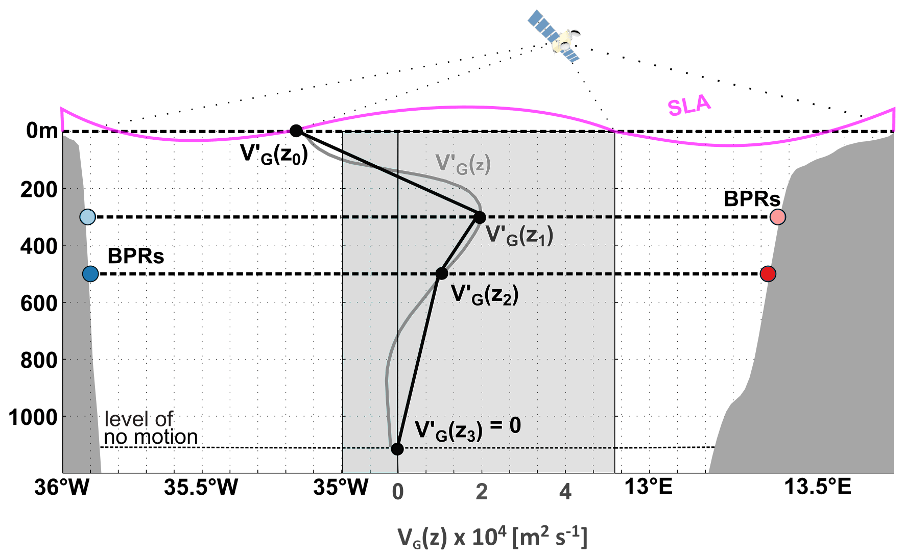
Figure 3 Experimental setup and strategy to estimate $T_{\mathrm{G}}^{\prime }$ showing the location of the BPRs (reddish and blueish circles) and the vertical sampling of $V_{\mathrm{G}}^{\prime }$. $V_{\mathrm{G}}^{\prime }$ is derived from measurements of sea level anomaly and with bottom pressure at 300 and 500 m depth. A level of no motion is prescribed to be at $z_{\mathrm{3}}=-\mathrm{1130}$ m. Two methods are used to approximate $V_{\mathrm{G}}^{\prime }\left(z\right)$: (i) piecewise linear interpolation of $V_{\mathrm{G}}^{\prime }$ between the four data points (black profile) and (ii) regression of the first and second dominant vertical structure functions of $V_{\mathrm{G}\mathrm{SIM}P\left(z\right)}^{\prime }$ from INALT01 onto the data points at 0, 300 and 500 m depth relaxing the no-flow condition at 1130 m depth (grey profile). $V_{\mathrm{G}}^{\prime }\left(z\right)$ is then vertically integrated from 1130 m to the surface to derive $T_{\mathrm{G}}^{\prime }$.

Following the observational strategy (Fig. 3), BPRs at least at four different locations (two depth levels) are required to derive basin-wide geostrophic transport variations in the upper 1130 m of the water column. While five recorders were in place over the period May 2014–October 2015, no BP measurements at 300 m depth off Brazil are available before May 2014 and none at all off Angola since November 2015. In this study, we found combined annual and semi-annual cycles explaining 44 %–61 % of the variance in the daily BP time series at the eastern boundary and 18 %–24 % of the variance at the western boundary (see Sect. 5.1). Despite the smaller numbers at the western boundary, the annual and semi-annual cycles are still the dominant signals in all pressure time series at 11^∘ S. Therefore, we decided to “replace” the missing sensors with the combined annual and semi-annual harmonics derived from the available BP time series. This means, for example, that the geostrophic transport after November 2015 is derived from the differences between measured BP variations at the western boundary and repeated annual and semi-annual harmonics – as derived from earlier years – at the eastern boundary. We derive confidence in our method from the comparison of the observed BP variations with variations in the simulated BP time series and in the SLA time series off Angola, both covering longer periods.

4.2 Using the INALT01 OGCM as a “testing area”

To validate our strategy for the computation of AMOC variations from the BP observations and to better understand the observed seasonal variability, we simultaneously analysed the output of the INALT01 OGCM (see Sect. 3). In INALT01, we can diagnose AMOC variations, $T_{\mathrm{AMOC}\mathrm{SIM}}^{\prime }$, from the velocity field using Eqs. (1) and (2), i.e. by directly integrating the simulated meridional velocity component at 11^∘ S horizontally across the basin and vertically from 1130 m to the surface. The zonally integrated Ekman transport T_EK SIM at 11^∘ S is derived with Eq. (7) from INALT01 wind stress. According to Eq. (6), the simulated upper-ocean geostrophic transport anomaly $T_{\mathrm{G}\mathrm{SIM}}^{\prime }$ is then $T_{\mathrm{AMOC}\mathrm{SIM}}^{\prime }-T_{\mathrm{EK}\mathrm{SIM}}^{\prime }$.

Alternatively, we can derive $T_{\mathrm{G}\mathrm{SIM}P\left(z\right)}^{\prime }$ according to our observational strategy based on BP fields from the modelled hydrographic fields and sea level. The model pressure field is given by

$$\begin{array}{}\text{(8)}& p\left(x,z,t\right)=g\cdot \underset{z}{\overset{\mathrm{0}}{\int }}\mathit{\rho }\left(x,z^{\prime },t\right)\mathrm{d}{z}^{\prime }+g\cdot {\mathit{\rho }}_{\mathrm{0}}\cdot \mathit{\eta }\left(x,t\right),\end{array}$$

with g being the acceleration of gravity, ρ the seawater density as function of z and η the sea level. Taking the BP along the continental slopes (at each depth level) of Brazil and Angola from Eq. (8), the simulated upper-ocean geostrophic transport anomalies, $V_{\mathrm{G}\mathrm{SIM}P\left(z\right)}^{\prime }$ and $T_{\mathrm{G}\mathrm{SIM}P\left(z\right)}^{\prime }$, can be derived from the pressure differences across the basin using Eqs. (3) and (5), respectively. Under the assumption that ageostrophic non-Ekman velocities are negligible, $T_{\mathrm{G}\mathrm{SIM}}^{\prime }$ and $T_{\mathrm{G}\mathrm{SIM}P\left(z\right)}^{\prime }$ should agree and particularly should show the same seasonal cycles. Additionally, we test the two methods used to approximate the vertical structure of $V_{\mathrm{G}}^{\prime }$ from the observations (see Sect. 4.1): (1) piecewise linear interpolation between values of $V_{\mathrm{G}\mathrm{SIM}P\left(z\right)}^{\prime }$ at 0, 300, 500 m depth and a level of no motion at 1130 m depth – denoted as $V_{\mathrm{G}\mathrm{SIM}\mathrm{Points}}^{\prime }$ or $T_{\mathrm{G}\mathrm{SIM}\mathrm{Points}}^{\prime }$ in the following and (2) regression of the first and second EOFs of $V_{\mathrm{G}\mathrm{SIM}P\left(z\right)}^{\prime }$ onto the values $V_{\mathrm{G}\mathrm{SIM}P\left(z\right)}^{\prime }$ at 0, 300, 500 m depth – deriving $V_{\mathrm{G}\mathrm{SIM}\mathrm{EOFs}}^{\prime }$ or $T_{\mathrm{G}\mathrm{SIM}\mathrm{EOFs}}^{\prime }$. These different transport estimates from INALT01 were used to validate the methods applied to the observations (see Sect. 5.3). In Sect. 5.4, we use INALT01 to identify relevant mechanisms of the seasonal AMOC variability at 11^∘ S, including specifically a comparison of the seasonal variability of the NBUC transport derived from observations and INALT01. For the sake of simplicity, in INALT01, unlike for the calculations from observations, the NBUC transport was calculated above a fixed depth of 1130 m and west of 34.55^∘ W.

5 Results

5.1 Ocean pressure variability at 11^∘ S

All of the ocean pressure time series in this study, i.e. at the surface from SLA (Fig. 2a, b), at 300 and 500 m depth from the BPRs (Fig. 1b), at the western or eastern boundary, are dominated by seasonal variability. The corresponding periodograms all exhibit pronounced peaks at periods of the annual and semi-annual cycles (coloured curves in Fig. 4).

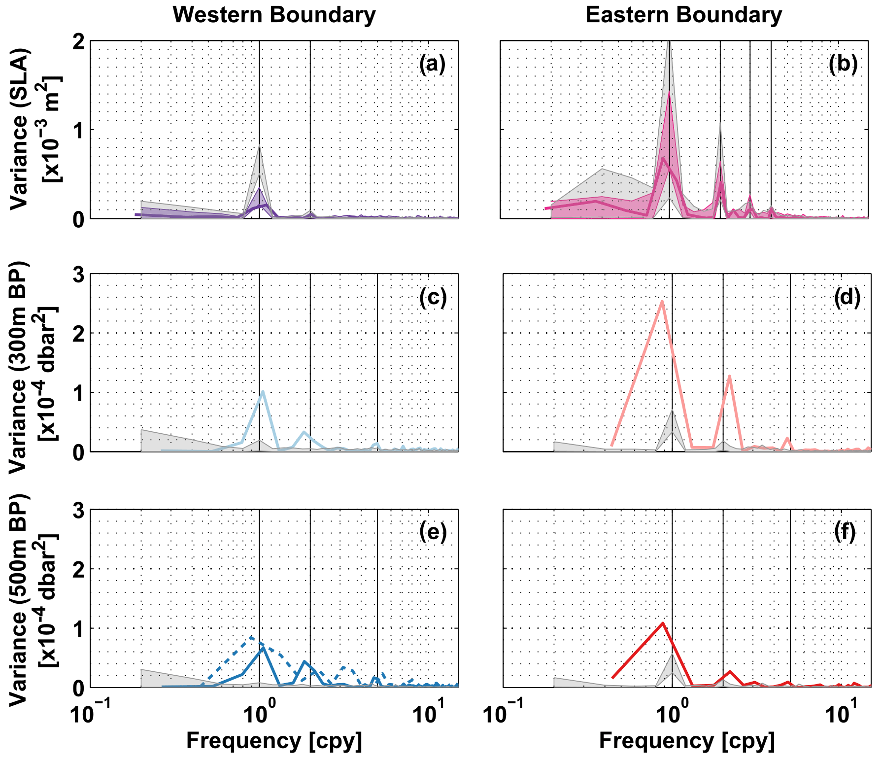
Figure 4 Periodograms of (a, b) SLA, (c, d) BP at 300 m and (e, f) BP at 500 m depth – from observations (coloured) and from the INALT01 model (grey). In panels (a, b), solid bold curves show periodograms calculated from SLA data over the period 2013–2018. The transparent envelopes are an estimate of interannual variations: specifically, the minimum and maximum ranges of periodograms calculated for 5-year windows running through the full available period (1993–2018). In panels (c, d, f), solid bold curves show periodograms calculated from the individual BP time series available at 11^∘ S. In panel (e), the solid curve represents KPO 1135 and the dashed curve KPO 1109 (two co-located sensors covering different periods; see Table 1). Grey shading in all panels gives the minimum and maximum ranges of periodograms for SLA and BP time series derived from the INALT01 model calculated for 5-year windows running through the full available period (1978–2007). Frequency is given in “cycles per year”. Vertical black lines mark the frequencies of the annual and semi-annual cycles, as well as periods of 120 and 90 d in panel (b) or 70 d in panels (c–f).

The main focus here is on seasonal variability; however, there are some other interesting peaks in the periodograms indicating energy on intraseasonal and interannual timescales. Off Brazil, variability at a period of 70 d (Fig. 4c, d) is very likely related to the DWBC eddies described by Dengler et al. (2004), which are thought to dominate the DWBC flow at 11^∘ S and influence the upper water column as well (e.g. Schott et al., 2005). The periodograms of SLA at the eastern boundary (Fig. 4b) exhibit peaks at 90 d, 120 d and 2 years. Variability at periods of 90 and 120 d was also observed by Kopte et al. (2018) in velocity time series from moored observations off Angola and is likely associated with the passage of CTWs. Based on numerical experiments, Bachèlery et al. (2016) showed that SLA variability along the African coast is on intraseasonal timescales (T<105 d) primarily driven by local atmospheric forcing, while at periods >120 d it can mostly be explained by equatorial forcing. Further, Polo et al. (2008) suggested that part of the intraseasonal variability is related to year-to-year variations of the seasonal cycle. Interestingly, the INALT01 OGCM does reproduce the spectral peaks at 2 years, 120 and 90 d in the SLA off Angola but not the 70 d period observed in any of the BP time series.

We found the relative importance of seasonal variability to be most pronounced near the surface off Angola in both the observations and the model (Fig. 4). The combined annual and semi-annual harmonics of the observed pressure time series explain most of the variance there – 61 % at the surface, 58 % at 300 m depth, 44 % at 500 m depth – and their amplitudes decrease with depth. To make this statement, we converted SLA variance into pressure variance using the hydrostatic equation. The combined annual and semi-annual harmonics at the eastern boundary (Fig. 5b, d, f) show a similar structure at different depths with maxima in austral autumn and spring, and a minimum in winter. Nevertheless, the phases of the annual and semi-annual cycles change with depth at different rates (Fig. 6). With a phase shift of about 5 months, the annual harmonics at the surface and 500 m depth are almost out of phase. The semi-annual harmonic is rather in phase, peaking about 1.5 months earlier at depth. This difference in the phase changes with depth can be associated with CTWs of certain baroclinic modes. Kopte et al. (2018) associated the annual and semi-annual cycles of the alongshore velocity from the mooring at 11^∘ S with basin-mode resonance in the equatorial Atlantic of the fourth and second baroclinic modes, respectively (Brandt et al., 2016). Corresponding CTWs propagate along the African coast towards 11^∘ S, thereby impacting the local velocity and pressure fields.

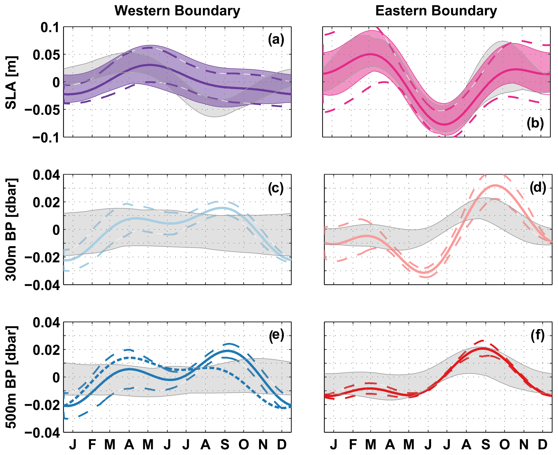
Figure 5 Combined annual and semi-annual harmonics calculated for (a, b) SLA, (c, d) BP at 300 m and (e, f) BP at 500 m depth. Line styles and colour coding are the same as in Fig. 4. Additionally, dashed envelopes around the solid curves give uncertainties for the amplitudes of the harmonics. These are calculated by 170 d low-pass filtering the pressure time series and then subsequently the 95th percentile of the deviations from the derived annual and semi-annual harmonics for every day of the year.

At the western boundary (Fig. 5a, c, e), the seasonal variability of the observed pressure time series is less pronounced. The combined annual and semi-annual harmonics explain only 12 % of the total variance at the surface and are barely different from zero, considering the uncertainty estimate of the amplitude. Seasonal variability of the surface pressure is decoupled from the pressure variability at depth, which supports the undercurrent character of the NBUC. The BP measurements at 300 and 500 m depth, which are both located in the depth range of the NBUC, have annual and semi-annual harmonics of similar amplitude and phase (Fig. 5d, f). The phase of the annual harmonic changes by 2 months between the surface and 300 m depth and the semi-annual harmonic by ∼ 1 month, and both peak later at depth (Fig. 5b, d). At depth, seasonal pressure variations also become more important; at 500 m depth, for example, the annual and semi-annual harmonics explain up to 29 %. We found similar results for 2-year subsets of the western boundary BP time series.

Annual and semi-annual harmonics of the individual pressure time series simulated in the INALT01 model (grey shading in Fig. 5) agree quite well with the observations regarding the timing of the maxima and minima. On the other hand, there are large differences in the amplitudes: the model tends to overestimate the annual harmonic at the surface and generally underestimate seasonal variability at depth – especially at the western boundary the seasonal cycle of the simulated BP at 300 and 500 m depth is almost non-existent.

In summary, for the seasonal variability at 11^∘ S, we observed that near the surface eastern boundary pressure variations prevail, whereas at 500 m depth the western and eastern boundary pressure variations are of similar importance. In the INALT01 model, the eastern boundary pressure variations dominate even more over western boundary ones.

5.2 Wind stress variability

Prevailing winds along 11^∘ S are from southeast, which results in a mean meridional Ekman transport toward south. Using wind stress derived from ASCAT for the period 2013–2018, the mean and standard error of the meridional Ekman transport amount to −11.7 ± 0.9 Sv and for the full available period (2007–2018) to −11.8 ± 0.6 Sv. The mean and standard error of the meridional Ekman transport derived from INALT01 wind stress amount to −10.7 ± 0.3 Sv. Zonal wind stress in the tropical South Atlantic varies on different timescales but is clearly dominated by seasonal variability. Periodograms of the Ekman transport based on ASCAT and INALT01 wind stress (Fig. 7a, b) both show the strongest peaks at the frequency of the annual cycle. Note that the two products cover very different periods and that their periodograms both also hint towards longer-term variability whenever considering the full records.

Figure 6 (a) Amplitudes and (b) phases of the minima of the annual (pluses and black curves) and semi-annual (crosses and grey curves) harmonics of the pressure anomalies at the eastern boundary along 11^∘ S. Markers represent estimates from the observations (2013–2018) at 0, 300 and 500 m; the curves show estimates calculated from INALT01 for 5-year windows running through the period of available data (1978–2007).

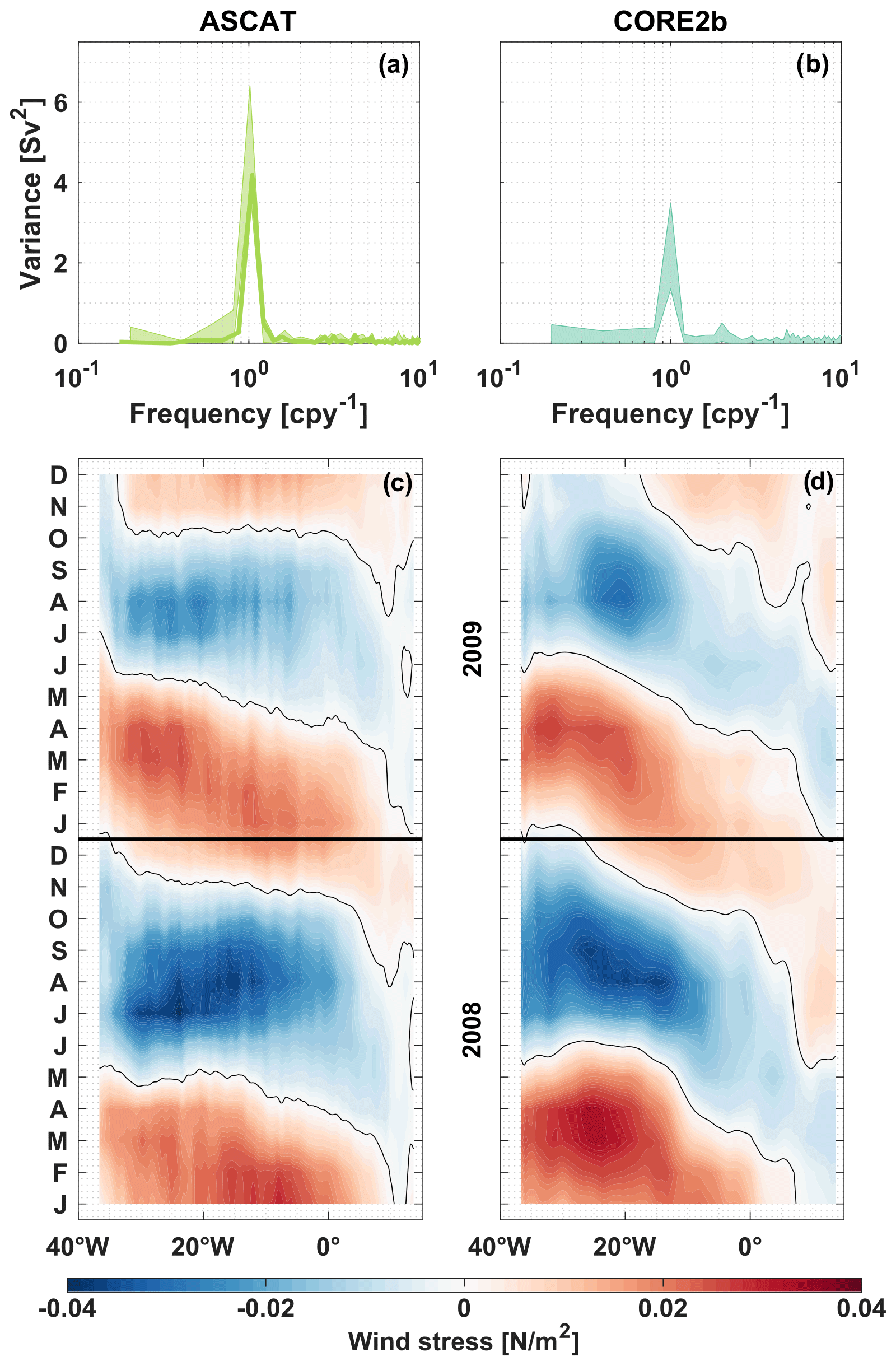
Figure 7 Periodograms of the Ekman transport at 11^∘ S, derived from ASCAT (a) and INALT01 (b) wind stress. The bold curve in panel (a) is calculated for the period 2013–2018. Transparent envelopes in panels (a–b) give an estimate of interannual variations: specifically, the minimum and maximum ranges of periodograms calculated for 5-year windows running through the full available time series of ASCAT (2008–2018) and INALT01 (1978–2009). Frequency is given in “cycles per year”. Hovmöller diagrams of the ASCAT (c) and INALT01 (d) zonal wind stress anomalies along 11^∘ S for the overlapping years (2008–2009). Red (blue) colours in (c–d) imply eastward (westward) wind stress anomalies.

The zonal wind stress anomalies at 11^∘ S for the two analysed wind products for the overlapping years (2008–2009) (Fig. 7c, d) agree in the following characteristics: seasonal wind stress variability is more pronounced in the western part of the basin than in the eastern part. Across the whole width of the basin, the zonal wind stress anomalies along 11^∘ S are typically eastward (positive) in January to March – resulting in a weaker basin-wide southward Ekman transport. In austral winter, zonal wind stress anomalies are rather westward (negative) and the southward Ekman transport is strongest – changing again towards the end of the year. For both wind products, the Ekman transport across 11^∘ S is mainly governed by the seasonal cycle of the southeasterly trade winds (e.g. Philander and Pacanowski, 1986). However, there are also recognizable differences between both products: for 2008–2009, the mean and the monthly standard deviation of the Ekman transport at 11^∘ S (not shown) are about 0.5 Sv larger for ASCAT than for INALT01, respectively. Wind stress anomalies along 11^∘ S reveal differences in its spatial structure, as well as in the course and amplitudes of its seasonal cycle (Fig. 7c, d).

5.3 Seasonal variability of the AMOC components at 11^∘ S

As described in the methods, we were able to estimate AMOC transport variations in the tropical South Atlantic from BP measurements over the period 2013–2018. Figure 8 displays the derived time series of $T_{\mathrm{G}}^{\prime }$, $T_{\mathrm{EK}}^{\prime }$ and the sum of both components $T_{\mathrm{AMOC}}^{\prime }$ at 11^∘ S. The different versions of $T_{\mathrm{G}}^{\prime }$ derived from four BPRs or from two to three BPRs complemented with the combined annual and semi-annual harmonics (Fig. 8a; see Sect. 4.1) show a general good agreement within the overlapping period. In the following sections, we analysed the combined time series of $T_{\mathrm{G}\mathrm{EOFs}\mathrm{2}\mathrm{BPRs}}^{\prime }$ (July 2013 to May 2014), $T_{\mathrm{G}\mathrm{EOFs}\mathrm{4}\mathrm{BPRs}}^{\prime }$ (May 2014 to November 2015) and $T_{\mathrm{G}\mathrm{EOFs}\mathrm{2}\mathrm{BPRs}}^{\prime }$ (November 2015 to March 2018; compare Fig. 8a).

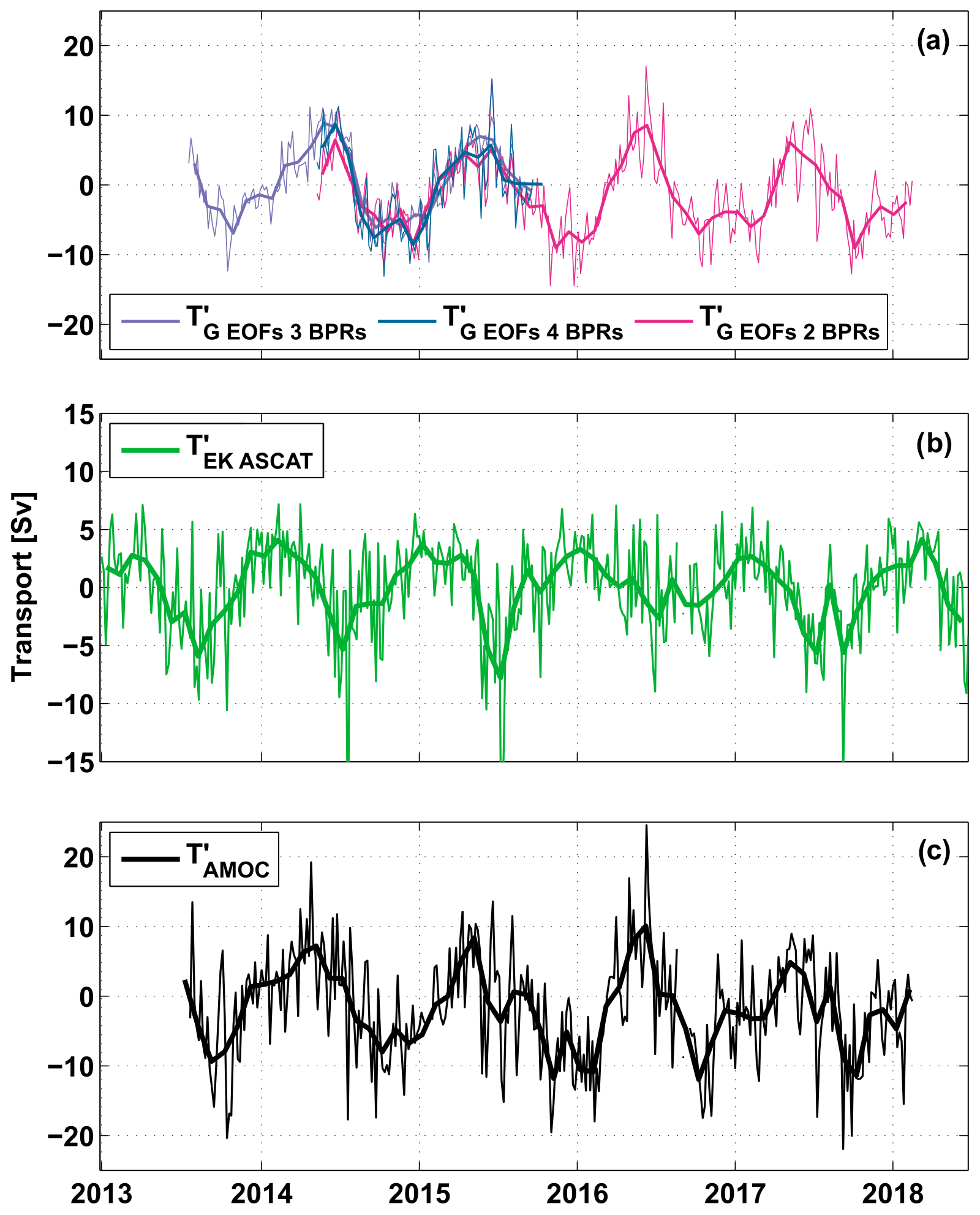
Figure 8 Anomaly time series at 11^∘ S of (a) the upper-ocean geostrophic transport ($T_{\mathrm{G}\mathrm{EOFs}}^{\prime })$, (b) the Ekman transport derived from ASCAT wind stress ($T_{\mathrm{EK}\mathrm{ASCAT}}^{\prime })$ and (c) the resulting AMOC transport ($T_{\mathrm{AMOC}}^{\prime })$. Thin lines represent daily values in panel (a) and 5 d values in panels (b, c); bold curves represent monthly averages. Different colours in panel (a) indicate transport calculations for different sets of BPRs – four BPRs (petrol), three BPRs (500 m WB, 300 m EB, 500 m EB; purple) and two BPRs (300 and 500 m WB; magenta) combined with the annual and semi-annual harmonics derived from the fully equipped period (May 2014–October 2015; see Sect. 4.1).

While from the BP observations we could only derive anomalies of T_G, in INALT01, we could also calculate mean values: the AMOC transport at 11^∘ S based on the INALT01 velocity field averaged over the whole model run (1978–2007) is T_AMOC SIM=14.1 ± 0.5 Sv (mean and standard error). This is within the uncertainty range of 3 Sv for the AMOC estimate of 16.2 Sv derived from a hydrographic ship section along 11^∘ S in 1994 (Lumpkin and Speer, 2007).

Both the $T_{\mathrm{G}}^{\prime }$ and $T_{\mathrm{EK}}^{\prime }$ time series, and hence also $T_{\mathrm{AMOC}}^{\prime }$, show variability on different timescales but are clearly dominated by seasonal variability. Mean seasonal cycles of $T_{\mathrm{G}}^{\prime }$, $T_{\mathrm{EK}}^{\prime }$ and $T_{\mathrm{AMOC}}^{\prime }$ from observations and INALT01 are shown in Fig. 9.

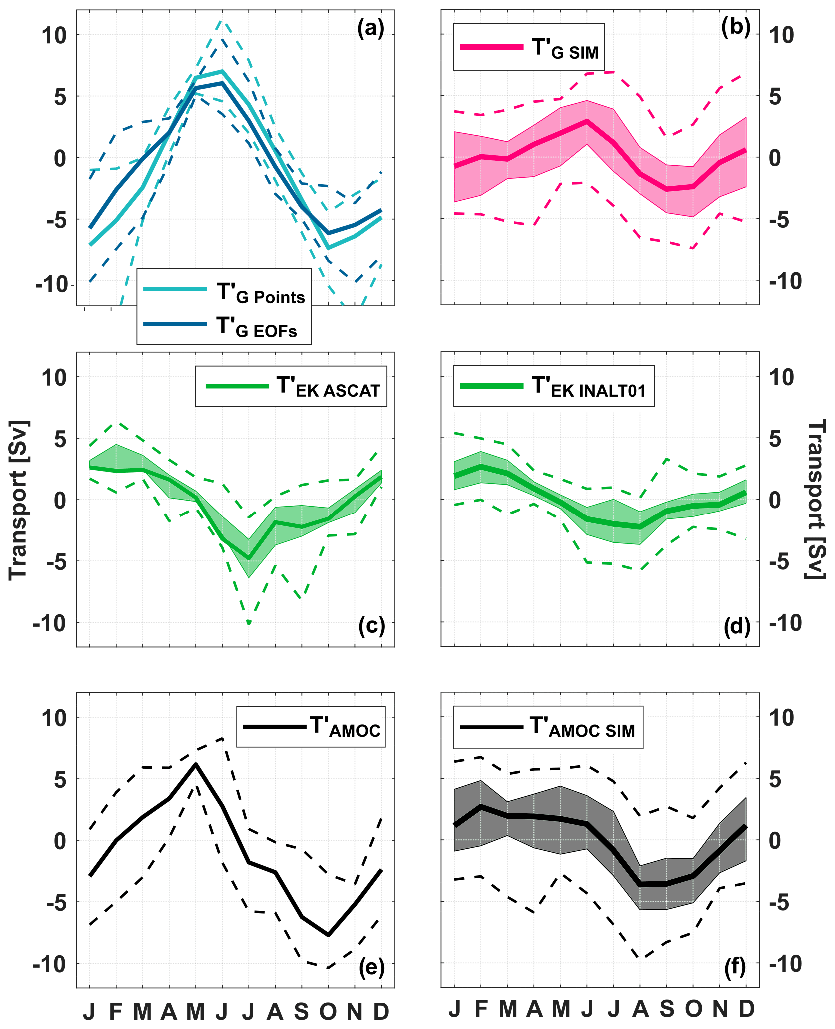
Figure 9 Mean seasonal cycles of $T_{\mathrm{G}}^{\prime }$ (a, b), $T_{\mathrm{EK}}^{\prime }$ (c, d) and $T_{\mathrm{AMOC}}^{\prime }$ (e, f) from observations (a, c, e) and the INALT01 model (b, d, f). Upper-ocean geostrophic transport anomalies, $T_{\mathrm{G}\mathrm{Points}}^{\prime }$ (cyan curve) and $T_{\mathrm{G}\mathrm{EOFs}}^{\prime }$ (petrol curve), are derived from SLA and BP observations (as described in Sect. 4.1) and averaged over the period 2013–2018, while $T_{\mathrm{G}\mathrm{SIM}}^{\prime }$, is derived from the INALT01 model velocity fields (as described in Sect. 4.2) and averaged over the period 1978–2007. $T_{\mathrm{AMOC}}^{\prime }$ in panel (e) was derived using $T_{\mathrm{G}\mathrm{EOFs}}^{\prime }$. For the 30-year INALT01 run (b, d, f) and the 12-year ASCAT wind time series (c), transparent envelopes represent an estimate of interannual variations: specifically, the minimum and maximum range of mean seasonal cycles calculated for 5-year windows running through the respective available periods. The dashed curves in all panels show the absolute range of possible minima and maxima per each month.

$T_{\mathrm{EK}}^{\prime }$ is characterized by a maximum southward transport in June–August and minimum southward transport in January–March, with the individual extrema slightly varying between ASCAT and INALT01 (Fig. 9c, d). Note again that both products are averaged over different periods. The peak-to-peak amplitude of seasonal Ekman transport variations is 7.1 Sv for ASCAT wind stress (2007–2018; Fig. 9c) and 4.9 Sv for INALT01 wind stress (1978–2009; Fig. 9d). The seasonal cycles may vary from year to year as well as on longer timescales. Here, such variations are, for example, estimated with the range of mean seasonal cycles calculated for running 5-year subsets of the available wind stress data: while the timing of the seasonal cycle of $T_{\mathrm{EK}}^{\prime }$ is rather stable between different periods, the peak-to-peak amplitudes have a range of 6–11 Sv for ASCAT and 2–8 Sv for INALT01.

The observed upper-ocean geostrophic transport anomaly ($T_{\mathrm{G}}^{\prime })$ shows a maximum northward transport in June, while minima occur in October and January with a weak secondary maximum in December (Fig. 9a, b). The two estimates, $T_{\mathrm{G}\mathrm{Points}}^{\prime }$ and $T_{\mathrm{G}\mathrm{EOFs}}^{\prime }$, referring to the two different methods, agree well in the timing of minima and maxima (Fig. 9a). However, the amplitude of the seasonal cycle of $T_{\mathrm{G}\mathrm{EOFs}}^{\prime }$, which we consider to be the more realistic solution in the following, is about 2 Sv smaller than the corresponding amplitude of $T_{\mathrm{G}\mathrm{Points}}^{\prime }$. A possible explanation for the difference between the two estimates based on observations is given below.

Nevertheless, the seasonal cycles of both estimates based on observations, $T_{\mathrm{G}\mathrm{Points}}^{\prime }$ and $T_{\mathrm{G}\mathrm{EOFs}}^{\prime }$, are substantially more pronounced than that of $T_{\mathrm{G}\mathrm{SIM}}^{\prime }$ derived directly from the velocity fields of the 30-year model run (Fig. 9b). The peak-to-peak amplitude of the seasonal cycle of $T_{\mathrm{G}\mathrm{SIM}}^{\prime }$ calculated over 30 years is 5.5 Sv, while amplitudes can range between 2 and 10 Sv when calculated for 5-year subsets. The peak-to-peak amplitude of $T_{\mathrm{G}\mathrm{EOFs}}^{\prime }$ calculated over the observed 4.5 years is 12.2 Sv and thus larger than the model range. Even when comparing the total range of possible seasonal cycles obtained by considering only single years, the observed values are just out of the range of the simulated values. Regarding the timing of minima and maxima, the observed and simulated seasonal cycles of $T_{\mathrm{G}}^{\prime }$ agree quite well (cf. Fig. 9a, b). The larger peak-to-peak amplitudes of the seasonal cycle of $T_{\mathrm{G}}^{\prime }$ from observations (cf. Fig. 9a, b) as well as the ASCAT Ekman transport (cf. Fig. 9c, d) result in a larger seasonal cycle of $T_{\mathrm{AMOC}}^{\prime }$ with a peak-to-peak amplitude of 13.9 Sv compared to $T_{\mathrm{AMOC}\mathrm{SIM}}^{\prime }$ (cf. Fig. 9e, f), which is 6.3 Sv calculated over 30 years and can be as large as 10.5 Sv when calculated for 5-year subsets.

In order to test our observational strategy, we compared the upper-ocean geostrophic transport anomaly derived directly from the simulated meridional velocity component ($T_{\mathrm{G}\mathrm{SIM}}^{\prime }$) to the one being derived from simulated BP time series. Using the full vertical resolution of the model when deriving $T_{\mathrm{G}\mathrm{SIM}P\left(z\right)}^{\prime }$, we obtained good agreement with $T_{\mathrm{G}\mathrm{SIM}}^{\prime }$ as expected (Fig. 10a and b). Reducing the vertical resolution to the depths of the pressure observations at 0, 300 and 500 m depth and using piecewise linear interpolation between those and a “level of no motion” at 1130 m ($V_{\mathrm{G}\mathrm{SIM}\mathrm{Points}}^{\prime }$; $T_{\mathrm{G}\mathrm{SIM}\mathrm{Points}}^{\prime }$; Fig. 10c, d), we found this method to miss certain parts of the vertical structure of $V_{\mathrm{G}\mathrm{SIM}P\left(z\right)}^{\prime }$ and, with that, to substantially overestimate the peak-to-peak amplitude of the seasonal cycle of $T_{\mathrm{G}\mathrm{SIM}P\left(z\right)}^{\prime }$ by 6 Sv (Fig. 10d). While in the model a strong seasonal cycle is confined to the near-surface ocean, linear interpolation between the surface and 300 m artificially increases the seasonal signal in the layer from 50 to 250 m depth. To improve the approximation, another method was applied that is based on a regression of the first and second dominant vertical structure functions of $V_{\mathrm{G}\mathrm{SIM}P\left(z\right)}^{\prime }$ onto the values at the three depth levels of pressure observations at 0, 300 and 500 m depth ($T_{\mathrm{G}\mathrm{SIM}\mathrm{EOFs}}^{\prime }$; $V_{\mathrm{G}\mathrm{SIM}\mathrm{EOFs}}^{\prime }$; Fig. 10e, f), thereby relaxing the no-flow condition at 1130 m depth. As the first two EOFs of $V_{\mathrm{G}\mathrm{SIM}P\left(z\right)}^{\prime }$ explain 99 % of the variance contained in $V_{\mathrm{G}\mathrm{SIM}P\left(z\right)}^{\prime }$, $T_{\mathrm{G}\mathrm{SIM}\mathrm{EOFs}}^{\prime }$ agrees well with $T_{\mathrm{G}\mathrm{SIM}P\left(z\right)}^{\prime }$ in INALT01 (Fig. 10f). However, the comparison of the observed BP time series with the BP simulated in INALT01 (Fig. 4) shows that the model tends to underestimate the seasonal pressure variability at depth (see Sect. 5.1), leaving some uncertainty regarding the vertical structure of $V_{\mathrm{G}}^{\prime }$ in reality.

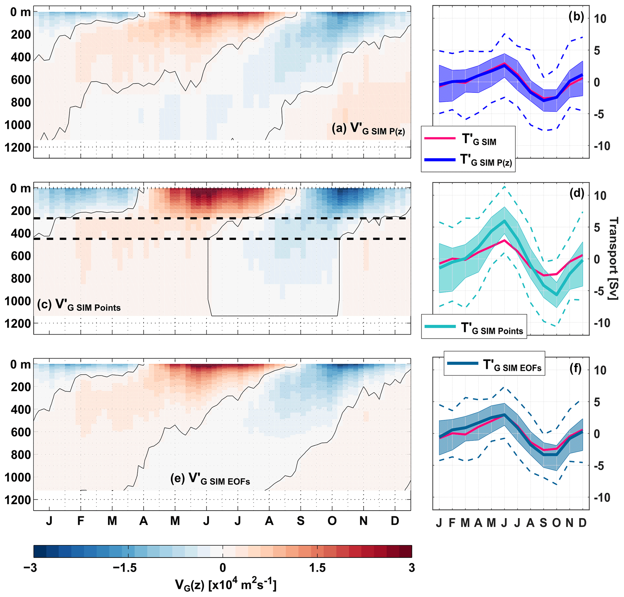
Figure 10 Mean seasonal cycles of the geostrophic transport per unit depth, $V_{\mathrm{G}\mathrm{SIM}}^{\prime }$ (a, c, e) and the upper-ocean geostrophic transport $T_{\mathrm{G}\mathrm{SIM}}^{\prime }$ (pink curves; b, d, f) from INALT01. $V_{\mathrm{G}\mathrm{SIM}P\left(z\right)}^{\prime }$ (a) and $T_{\mathrm{G}\mathrm{SIM}P\left(z\right)}^{\prime }$ (blue curve; b) were calculated using the full vertical profiles of BP. $V_{\mathrm{G}\mathrm{SIM}\mathrm{Points}}^{\prime }$ (c) and $T_{\mathrm{G}\mathrm{SIM}\mathrm{Points}}^{\prime }$ (cyan curve; d) were reconstructed by piecewise linear interpolation of $V_{\mathrm{G}}^{\prime }$ between the four supporting points at 0, 300, 500 and 1130 m depth (dashed black lines in panel c mark the depths of the BPRs); $V_{\mathrm{G}\mathrm{SIM}\mathrm{EOFs}}^{\prime }$ (e) and $T_{\mathrm{G}\mathrm{SIM}\mathrm{EOFs}}^{\prime }$ (petrol curve; f) by using the dominant vertical structure functions from INALT01. In panels (a, c, e), red (blue) colours show northward (southward) anomalies.

Figure 11 compares the mean seasonal cycles of $V_{\mathrm{G}}^{\prime }$ from observations for the two different methods. Using the vertical structure from the EOFs of $V_{\mathrm{G}\mathrm{SIM}P\left(Z\right)}^{\prime }$ from INALT01 especially reduces the amplitude of the subsurface variability (50–200 m). In this depth range, the transition from negative to positive transport anomalies also shifts from April to March. At larger depths, differences between both methods are the result of $V_{\mathrm{G}\mathrm{Points}}^{\prime }$ being constrained by a level of no motion at 1130 m, while $V_{\mathrm{G}\mathrm{EOFs}}^{\prime }$ is not. However, independent of the applied method, the peak-to-peak amplitude of the seasonal cycle of $T_{\mathrm{G}}^{\prime }$ from observations (Fig. 9a) remains to be substantially larger than that from INALT01.

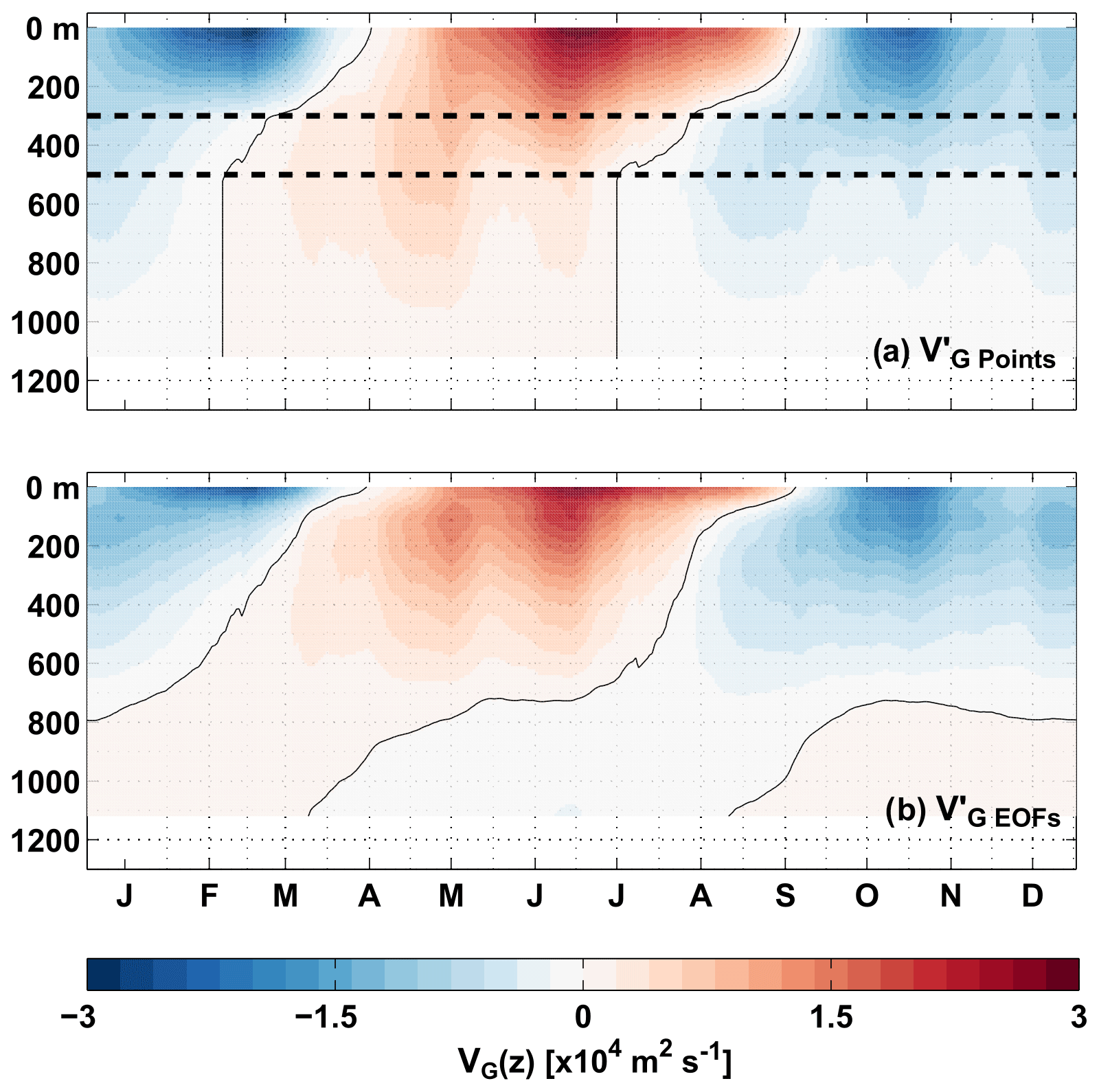
Figure 11 Mean seasonal cycle of the geostrophic transport per unit depth, $V_{\mathrm{G}}^{\prime }$, over the period 2013–2018, derived from observations at 11^∘ S with two methods: (a) piecewise linear interpolation between the four supporting points at 0, 300, 500 and 1130 m depth (dashed black lines mark the depths of the BPRs). (b) Reconstruction of $V_{\mathrm{G}}^{\prime }$ by regression of the dominant vertical structure functions from the INALT01 model onto the values at the three depth levels of pressure observations at 0, 300 and 500 m depth, thereby relaxing the no-flow condition at 1130 m depth. Red (blue) colours show northward (southward) anomalies.

For the period 2013–2018, the geostrophic contribution to the seasonal cycle of the AMOC at 11^∘ S, as we observed it, exceeds the Ekman contribution almost by a factor of 2 (cf. Fig. 9a, c). In INALT01, on the other hand, averaged over the 30-year model run, the geostrophic and Ekman contributions are of similar magnitude (Fig. 9b, d). The seasonal cycles of both contributions vary substantially between years (calculated for 5-year subsets of the model run), e.g. 2–10 Sv for $T_{\mathrm{G}\mathrm{SIM}}^{\prime }$ from INALT01, 2–8 Sv for $T_{\mathrm{EK}}^{\prime }$ from INALT01 or 6–11 Sv for $T_{\mathrm{EK}}^{\prime }$ from ASCAT; hence, there is a modulation of the ratios of both contributions on interannual timescales. However, even when considering the uncertainties of the seasonal cycle of $T_{\mathrm{G}\mathrm{Points}}^{\prime }$ or $T_{\mathrm{G}\mathrm{EOFs}}^{\prime }$ (Fig. 9a) and the range of possible mean seasonal cycles of $T_{\mathrm{G}\mathrm{SIM}}^{\prime }$ calculated for subsets of the model run (Fig. 9b), the observed values are significantly larger than simulated ones.

5.4 Dynamics of the seasonal cycle at 11^∘ S

In order to better understand the mechanisms that set the seasonal cycle of $T_{\mathrm{AMOC}}^{\prime }$ at 11^∘ S, we investigated the longitudinal structure of the geostrophic velocity field and transport along that section in INALT01. We were able to distinguish three different regimes – the NBUC, the western basin interior and the eastern basin – all showing seasonal variability of similar magnitude (Fig. 12).

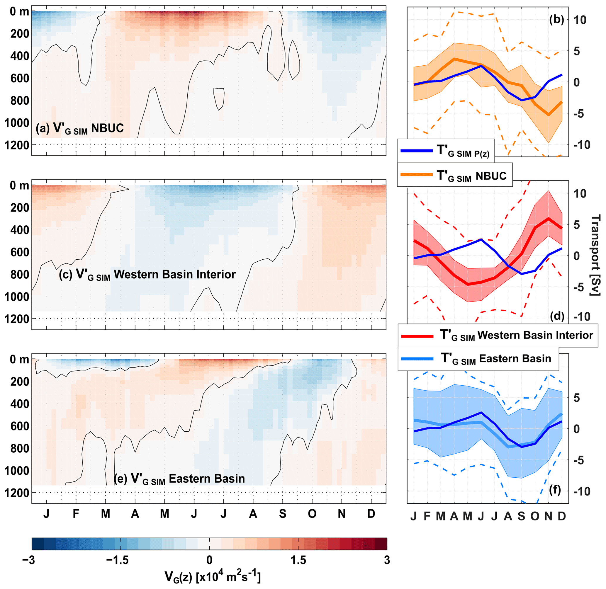
Figure 12 Mean seasonal cycle of the geostrophic transport per unit depth, $V_{\mathrm{G}\mathrm{SIM}}^{\prime }$ (a, c, e) and the upper-ocean geostrophic transport $T_{\mathrm{G}\mathrm{SIM}}^{\prime }$ (b, d, f) from INALT01. In all panels, $V_{\mathrm{G}}^{\prime }$ and $T_{\mathrm{G}}^{\prime }$ were calculated from the full vertical profiles (from the surface down to 1130 m) of the simulated pressure but from pressure differences across different regions along 11^∘ S: across the whole basin ($T_{\mathrm{G}\mathrm{SIM}P\left(z\right)}^{\prime }$; blue curves in panels b, d, f); between the Brazilian continental slope and 34.55^∘ W ($V_{\mathrm{G}\mathrm{SIM}}^{\prime }$ NBUC in panel a); $T_{\mathrm{G}\mathrm{SIM}}^{\prime }$ NBUC orange curves in panel (b); between 34.55^∘ W and 10^∘ W ($V_{\mathrm{G}\mathrm{SIM}}^{\prime }$ western basin interior in panel c; $T_{\mathrm{G}\mathrm{SIM}}^{\prime }$ western basin interior; red curves in panel d); between 10^∘ W and the Angolan continental slope ($V_{\mathrm{G}\mathrm{SIM}}^{\prime }$ eastern basin in panel e; $T_{\mathrm{G}\mathrm{SIM}}^{\prime }$ eastern basin; light blue curve in panel f). Transparent shading and dashed curves are the same as in Fig. 9.

The mean seasonal cycle of the NBUC, as calculated for the 30-year INALT01 model run, has its maximum in April, minimum in November and a peak-to-peak amplitude of 10 Sv (Fig. 12b). Peak-to-peak amplitudes of up to 15 Sv can be found in 5-year subsets of the model time series. Having a mooring array installed off the coast off Brazil measuring the Western Boundary Current system there (e.g. Hummels et al., 2015; see Sect. 2.4) allowed us to directly compare the seasonal variability of the NBUC in INALT01 with observations. The seasonal cycle of the NBUC in INALT01 agrees quite well with the seasonal cycle observed in recent years – regarding the peak-to-peak amplitude (7.6 Sv in 2000–2004 and 7 Sv in 2013–2018) and the timing of maximum and minimum transport (Fig. 13b). During the earlier deployment period (2000–2004), there was a stronger semi-annual cycle, creating a secondary minimum in March, which was neither found in the observations during 2013–2018 nor in INALT01.

In INALT01, the contribution of the NBUC to the AMOC on seasonal timescales is largely compensated by the flow in the western basin interior. The seasonal cycle of the geostrophic transport per unit depth in the western basin interior is of similar strength and vertical structure but of opposing sign to the one of the NBUC (cf. Fig. 12a, c). In the western basin interior, the vertically integrated upper-ocean geostrophic velocity is mainly associated with an annual harmonic and likely related to a strong seasonal cycle in the local wind stress curl (Fig. 14). The annual harmonic of the wind stress curl exhibits relatively large amplitudes over the region (10 to 34.55^∘ W) and a westward phase propagation (not shown).

As the contributions of the NBUC and western basin interior seasonal cycles to the AMOC tend to cancel each other out, in INALT01, seasonal variability of the upper-ocean geostrophic transport at 11^∘ S is mainly set in the eastern basin (Fig. 12f). Both the vertically integrated upper-ocean geostrophic velocity and the wind stress curl (Fig. 14) exhibit strong seasonal variability throughout most of the eastern basin. However, the largest amplitudes of the annual and semi-annual harmonics of the vertically integrated upper-ocean geostrophic velocity are found near the eastern boundary, east of 12^∘ E, where seasonal variability in the wind stress curl is weak.

From this analysis, we conclude that a compensation between the NBUC and western basin interior results in a major contribution of the upper-ocean geostrophic transport of the eastern basin to the AMOC transport on seasonal timescales. As described in Sect. 5.1, however, the model tends to underestimate the seasonal pressure variability at 300 and 500 m depth – especially at the western boundary. This leaves some uncertainty in the relative importance of western and eastern basin contributions to the seasonal AMOC variability in reality.

6 Summary and discussion

In this study, we used bottom pressure observations on both sides of the basin at 300 and 500 m depth, combined with satellite measurements of sea level anomalies, different wind stress products and model results, to estimate the upper-ocean geostrophic and Ekman transport contributions to AMOC variability at 11^∘ S over the period 2013–2018.

The use of bottom pressure measurements to compute basin-wide integrated northward transport is not straightforward: firstly, the sensors experience instrumental drifts, which limits the BPRs capabilities to recover variability on longer timescales. Secondly, the deployment depth is not precisely known, which only allows the calculation of transport anomalies. We found the available BP time series at 11^∘ S to be sufficiently long to investigate the seasonal variability in the region, but, clearly, longer time series will allow us to refine these estimates in the future.

At 11^∘ S, seasonal variability is strong in most of the time series presented in this study. After removing tides with periods shorter than 35 d, the combined annual and semi-annual harmonics explain a large part of the variability at the eastern boundary – from 60 % at the surface to 44 % at 500 m depth. We found hints towards a baroclinic structure in the annual and semi-annual harmonics of the pressure time series at the eastern boundary (Fig. 6), which could be related to CTWs of specific baroclinic modes that can travel from the Equator towards 11^∘ S along the African coast, thereby impacting the local pressure and velocity fields.

At the western boundary, seasonal pressure variability is weaker with its relative importance compared to other variability increasing with depth; the annual and semi-annual harmonics explain about 10 % of the variability at the surface and 30 % at 500 m depth. The seasonal variability of the zonally integrated geostrophic velocity anomaly in the upper 300 m is therefore mainly controlled by pressure variations at the eastern boundary, while at 500 m depth contributions from the western and eastern boundaries are similar. Annual and semi-annual harmonics at the western boundary also exhibit a vertical structure as seasonal variability at the surface is decoupled from the pressure variability at 300 and 500 m depth. Based on geostrophic velocity fields from hydrographic measurements, studies like da Silveira et al. (1994) or Stramma et al. (1995) already stated that the WBC system at 11^∘ S includes an energetic undercurrent, the NBUC, with weak or reversed flow above. From moored observations, Schott et al. (2005) showed strong gradients in the amplitude of the annual harmonic in the upper few hundred metres of the water column (their Fig. 11a), suggesting a decoupling of the variability at the surface from the subsurface.

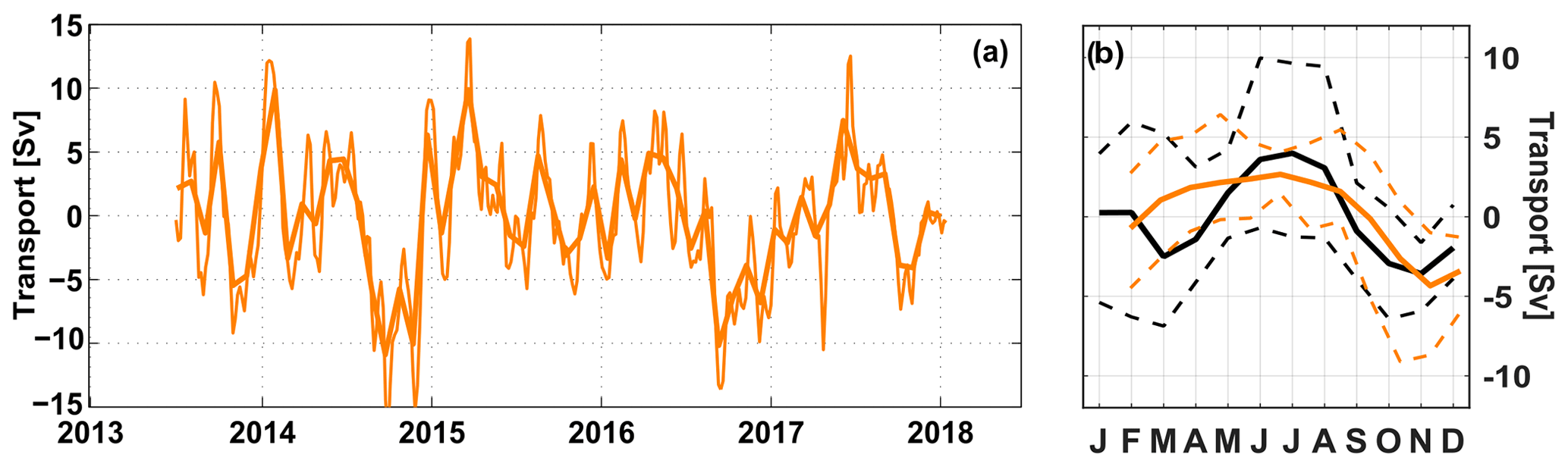
Figure 13 (a) Time series of NBUC transport anomalies (5-daily as thin curve and monthly averages as bold curve) based on moored observations off Brazil (see Sect. 2.4) updated from Schott et al. (2005) and Hummels et al. (2015). (b) Mean seasonal cycles of the NBUC transport anomalies averaged over the periods 2013–2018 (orange curve) and 2000–2004 (black curve). The thin dashed curves show the absolute range of possible minima and maxima per each month for the periods 2013–2018 (orange) and 2000–2004 (black), respectively.

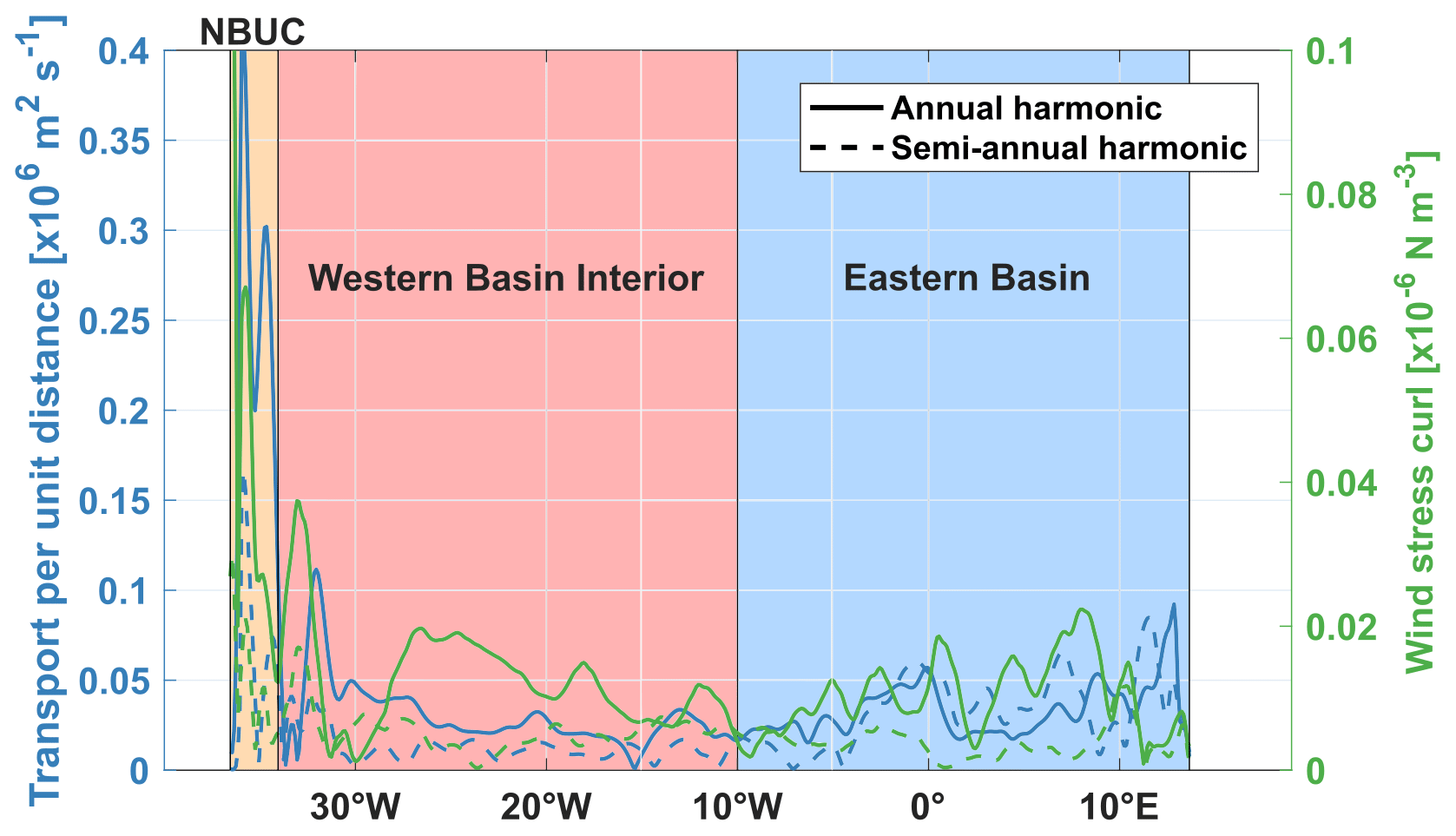
Figure 14 Amplitudes of the annual (solid curves) and semi-annual (dashed curves) harmonics of the vertically integrated upper-ocean geostrophic velocity in INALT01 (blue curves; left axis) and the INALT01 wind stress curl (green curves; right axis) along 11^∘ S. Transparently shaded boxes highlight different regions – the NBUC (orange), the western basin interior (red) and the eastern basin (blue).

Over the period 2013–2018, the upper-ocean geostrophic transport variations derived from pressure differences across the basin are dominated by seasonal variability – with a peak-to-peak amplitude of 12–14 Sv, depending on the method used to approximate its vertical structure. The peak-to-peak amplitude of the mean seasonal cycle of the Ekman transport is 7 Sv and of the resulting AMOC transport 14–16 Sv. For the subtropics, recent estimates of the peak-to-peak amplitude of the mean seasonal cycle of the AMOC range from 4.3 Sv at 26.5^∘ N (2004–2017; Frajka-Williams et al., 2019) to 13 Sv at 34.5^∘ S (2014–2017; Kersalè et al., 2020).

The output of the INALT01 OGCM was compared to the observed characteristics of the seasonal cycles of the AMOC, its components as well as the NBUC. It reproduces the seasonal cycles of the NBUC as observed in recent years with current meter moorings and of the Ekman transport across 11^∘ S, as derived from ASCAT winds. However, this comparison also reveals model–observation discrepancies regarding seasonal variability in the bottom pressure fields and the resulting geostrophic transport variations.

The INALT01 model tends to underestimate the seasonal bottom pressure variability at 300 and 500 m, especially at the western boundary. This translates into the vertical structure of the simulated geostrophic transport variations, which is also used for the calculation of the observational estimate (method 2) adding to its uncertainty.

In the observations, the geostrophic contribution to seasonal AMOC variability exceeds the Ekman contribution by almost a factor of 2, while in INALT01, averaged over the 30-year model run, or in earlier studies based on models (e.g. Zhao and Johns, 2014), the contributions are similar. Even when considering the multi-year variations of the seasonal cycle of $T_{\mathrm{G}}^{\prime }$ over 2013–2018 (Fig. 9a) and the total range of possible seasonal cycles of $T_{\mathrm{G}\mathrm{SIM}}^{\prime }$ calculated for subsets of the model run period (1978–2007) (Fig. 9b), the observed values are significantly larger than the simulated values.

The ratios of the NBUC and AMOC seasonal amplitudes are different between the observations (<1) and the model (>1).

In the model, seasonal upper-ocean geostrophic transport variability at 11^∘ S is governed by the variability in the eastern basin. The seasonal cycle of the simulated upper-ocean geostrophic transport in the western basin becomes comparable small due to a compensation of the western basin interior and the NBUC transport. This could be explained by an almost equilibrium response of the circulation in the western basin at low baroclinic modes to the wind stress curl (e.g. Döös, 1999). Locally wind-forced annual Rossby waves would travel westward and after arriving at the western boundary directly force WBC variability. The seasonal variability in the eastern basin is instead forced by the local wind stress curl and, additionally, by Rossby waves radiated from the eastern boundary via poleward propagation of seasonal CTWs (e.g. Brandt et al., 2016; Kopte et al., 2018). Similar Rossby-wave radiation from the eastern boundary has been reported for the tropical North Atlantic (e.g. Chu et al., 2007) and proposed to be one of the main mechanisms for seasonal variations in the geostrophic transport there (e.g. Hirschi et al., 2006; Zhao and Johns, 2014).

The compensation between the western basin interior and the NBUC on seasonal timescales found in INALT01 results in a minor contribution of the western basin compared to the eastern basin and limits the importance of the NBUC for AMOC variability on seasonal timescales. However, in this study, we found that INALT01 tends to underestimate seasonal variability at 300 and 500 m off Brazil. In two different model studies, Rodrigues et al. (2007) and Silva et al. (2009) related seasonal variability in the NBUC to seasonal variations in the bifurcation region of the South Equatorial Current. Thus, the phases of the annual and semi-annual harmonics of the NBUC may not simply be set by the response to the local wind curl forcing in the western basin at 11^∘ S but may also depend on the wind curl forcing further south and associated equatorward signal propagation along the western boundary.

We conclude that the seasonal variability of the geostrophic contribution to the AMOC at 11^∘ S is mainly wind forced, as it is modulated by oceanic adjustment to local and remote wind forcing. While some of the uncertainties of our analysis result from the technical aspects of the observational strategy or processes being not properly represented in the model, our results indicate that uncertainties in the wind forcing are particularly relevant for AMOC estimates in the tropical South Atlantic. Differences between wind products are an important source of uncertainty for estimates of the AMOC and its variability. Especially when comparing estimates of AMOC strength and variability between different projects, latitudes or from observations and models, the choice of wind product is crucial.

This study adds to the overall understanding of local and shorter-term AMOC variations, which is important for estimating the significance of long-term AMOC changes and thus for the detectability of its meridional coherence. To predict the long-term behaviour of the AMOC and its impacts, continuous observations from purposefully designed arrays are required in different key locations. We would like to argue that the observational programme at 11^∘ S, if continued into the future, has potential for monitoring long-term AMOC changes. As the western tropical Atlantic is a crossroad for the different branches of the AMOC and a region with high signal-to-noise ratios, 11^∘ S is a good place to monitor AMOC variations. Having a sustainable AMOC observing system there, linking northern and southern AMOC variability, would contribute to the general understanding of related mechanisms. There is potential to use the BPRs for investigating longer-term AMOC variability. While progress is made in solving the problems of bottom pressure sensors on longer timescales (e.g. Kajikawa and Kobata, 2014; Worthington et al., 2019), the advantage of our method is that the BPRs are less expensive and easier to deploy than full-height mooring arrays. Learning from the use of long-term PIES arrays at 47^∘ N (Roessler et al., 2015) or 34.5^∘ S (e.g. Meinen et al. 2018), we think that the travel times derived from the PIES installed off Brazil could add information to or reduce the uncertainty of our results. Additionally, we can fall back on more than 20 years of shipboard hydrographic measurements in the tropical South Atlantic – at the western (e.g. Hummels et al., 2015; Herrford et al., 2017) and eastern boundaries (e.g. Tchipalanga et al., 2018). Ongoing work includes combining all of these hydrographic measurements to extend the time series of the WBC system and AMOC at 11^∘ S back into the 1990s.