Winter observations alter the seasonal perspectives of the nutrient transport pathways into the lower St. Lawrence Estuary

The St. Lawrence Estuary connects the Great Lakes with the Atlantic Ocean. The accepted view, based on summer conditions, is that the estuary's surface layer receives its nutrient supply from vertical mixing processes. This mixing is caused by the estuarine circulation and tides interacting with the topography at the head of the Laurentian Channel. During winter when ice forms, historical process-based studies have been limited in scope. Winter monitoring has been typically confined to vertical profiles of salinity and temperature as well as near-surface water samples collected from a helicopter for nutrient analysis. In 2018, however, the Canadian Coast Guard approved a science team to sample in tandem with its ice-breaking and ship escorting operations. This opportunistic sampling provided the first winter turbulence observations, which covered the largest spatial extent ever measured during any season within the St. Lawrence Estuary and the Gulf of St. Lawrence. The nitrate enrichment from tidal mixing resulted in an upward nitrate flux of about 30 nmol m⁻² s⁻¹, comparable to summer values obtained at the same tidal phase. Further downstream, deep nutrient-rich water from the gulf was mixed into the subsurface nutrient-poor layer at a rate more than an order of magnitude smaller than at the head. These fluxes were compared to the nutrient load of the upstream St. Lawrence River. Contrary to previous assumptions, fluvial nitrate inputs are the most significant source of nitrate in the estuary. Nitrate loads from vertical mixing processes would only exceed those from fluvial sources at the end of summer when fluvial inputs reach their annual minimum.

1 Introduction

Oceans, coastal seas, and estuaries at high latitudes are relatively under-sampled due to their isolation and inhospitable weather. Ambitious multidisciplinary campaigns have been undertaken in the Canadian Arctic aboard the icebreaker CCGS Amundsen, such as CASES (Fortier et al., 2008), CFL (Barber et al., 2010), and Arctic SOLAS (Papakyriakou and Stern, 2011–2012), but few scientific campaigns have been carried out in the St. Lawrence Estuary and the Gulf of St. Lawrence during the sea-ice season (Fig. 1). Estuaries are productive ecosystems where fresh water from the land meets water from the ocean. The St. Lawrence, for example, connects the Great Lakes to the Atlantic Ocean and represents an essential resource for Canada's economy (Archambault et al., 2017). Here, we present winter measurements collected alongside the coast guard's normal icebreaker operations. We were unsure what to expect from our winter mixing measurements, but the low nutrient uptake through photosynthesis provided a better representation of the nutrient transport mechanisms than possible from summer observations.

The accepted view is that nutrients in the surface layer of the lower St. Lawrence Estuary originate from tidal-induced upwelling and internal waves at the head of the channel (Ingram, 1975, 1983; Cyr et al., 2015) and/or entrainment of deep nutrient-rich water from the estuarine circulation as fluvial waters from the upper estuary flow to the sea (e.g., Steven, 1971). The magnitude and impact of these two vertical mixing processes on primary production across the whole lower estuary and gulf system are debated amongst observational and modeling studies (e.g., Cyr et al., 2015; Savenkoff et al., 2001; Jutras et al., 2020). Published observations for the St. Lawrence have typically focused on the nutrient transport from vertical mixing dynamics within the lower estuary instead of the fluvial loads. These loads are caused by the horizontal advection of fluvial waters that drain the Great Lakes between Canada and the USA – notably the urbanized catchment upstream of Quebec City (Hudon et al., 2017).

Using field observations, Cyr et al. (2015) quantified the nitrate supply at the head of the channel from vertical mixing processes in late summer with direct turbulence measurements. Their measured nitrate vertical fluxes ranged between 0.2 and 3.5 $\mathrm{\mu }\mathrm{mol}{\mathrm{m}}^{-\mathrm{2}}{\mathrm{s}}^{-\mathrm{1}}$ (95 % bootstrapped confidence intervals). These estimates represent the world's highest reported vertical fluxes (see Table 1 of Cyr et al., 2015). Their estimates are also large compared to the global distribution of fluxes obtained by an ocean model (Fig. 5 of Mouriño-Carballido et al., 2021). The map by Mouriño-Carballido et al. (2021) also illustrates the lack of vertical nitrate flux measurements worldwide and the high fluxes obtained in the lower estuary during summer. The lower estuary's fluxes are an order of magnitude higher than those reported for the Mauritanian upwelling region – renown for being one of the most biologically productive in the world (Schafstall et al., 2010). Cyr et al. (2015) also estimated the nitrate enrichment elsewhere in the lower estuary from shear-induced mixing at the base of the nitricline. By combining this estimate with those at the head, they estimated that between 33 and 400 mol s⁻¹ of nitrate was being transported into the lower estuary's surface layer by vertical mixing processes. These summer estimates were not compared to fluvial nutrient inputs from upstream. Previous moored observations have shown that internal waves and tidal mixing processes are still present at the head of the channel during winter (Smith et al., 2006). Thermosalinograph observations show that these mixing processes generate warmer waters during winter and cooler water during summer (see Fig. 10 of Galbraith et al., 2019). However, the mixing and vertical nitrate fluxes have not been measured anywhere in the estuary during winter.

Biogeochemical box models have been used to evaluate the importance of vertical mixing processes in supplying nutrients into the lower estuary's surface (e.g., Savenkoff et al., 2001; Jutras et al., 2020). These box models consider the fluvial nutrients advected into the lower estuary. These steady-state models also assume that the estuarine circulation of the lower estuary can be idealized using a few homogeneous layers. Savenkoff et al. (2001) created an inverse box model using four layers that also separated the entire lower estuary and gulf region into eight different zones. Vertical mixing processes brought 685 mol s⁻¹ near the surface of the lower estuary – more than 5 times fluvial waters (Figs. 6 and 10 of Savenkoff et al., 2001). Jutras et al. (2020) revisited the nutrient loads with a three-layer model representative of the lower estuary's summer conditions. Their vertical flux of dissolved nitrogen in the surface (1050 mol s⁻¹) was 3 times larger than the contributions from fluvial sources. Both box-modeling studies estimated vertical fluxes of nitrogen (nitrate) that were much larger than those obtained directly by Cyr et al. (2015) in the field. Neither considered winter conditions.

We quantify the nutrient transport from diverse pathways, such as fluvial advection and vertical mixing in the estuary. We evaluate their relative importance for creating a nutrient inventory in the upper water column during winter, which sets up the subsequent spring bloom. We also extend the analysis to other seasons and revisit the importance of fluvial inputs for supplying nutrients into the St. Lawrence Estuary throughout the year. Our analysis ignores nutrient cycling within the system or any export through advective processes. The goal is to compare the fluvial nitrate loads with those entering the box from vertical mixing processes.

Figure 1 (a) Map of the estuary and the Gulf of St. Lawrence along with the stations visited with VMPs indicated by red squares and CTD profiles with black × symbols. Station L96 coincides with a long-term monitoring station of Fisheries and Oceans Canada's Atlantic Zone Monitoring Program (AZMP), Rimouski station. (b) Enlargement of the magenta inset in (a) to illustrate the head of the channel region and two Saguenay stations surveyed by helicopter in March 2018.

2 Study site and observations

2.1 Site description

The St. Lawrence seaway connects the Great Lakes to the Atlantic Ocean, with the extensive Saguenay–St. Lawrence Marine Park at the head of the Laurentian Channel (HLC). The ∼400 m deep Laurentian Channel rises sharply at the HLC (Fig. 1b). The head denotes the upstream extent of the lower estuary where the shallow upper estuary ends. At the HLC, the strong barotropic tide (up to 5 m amplitude) interacts with the ≈80 m sill and generates intense tidal upwelling. This interaction generates internal waves at tidal and higher frequencies, breaking lee waves, Kelvin–Helmholtz instabilities, and internal hydraulic jumps (Saucier and Chassé, 2000). The head of the channel was first hypothesized by Ingram (1975, 1983) to be a turbulent mixing hot spot that supplies nutrients for primary production in the lower estuary. Others considered the importance of the estuarine circulation in entraining nitrate-rich waters below the mixed surface layer into the surface layer (Steven, 1971, 1974; Sinclair et al., 1976). Throughout most of the year, the lower estuary's circulation is characterized by a surface layer outflowing above a weaker inflow in the intermediate layer and even weaker inflow in the deep waters below about 150 m (see Fig. 2 of Sinclair et al., 1976). The surface outflow therefore becomes saltier as it moves seawards.

The lower estuary progressively widens until reaching the gulf that begins at Pointe-des-Monts (Fig. 1a). At the most seaward eastern extent of the St. Lawrence system, Cabot Strait is where warmer and saltier waters from the Atlantic enter near the bottom. These waters form by the warm subtropical waters transported north by the Gulf Stream, which mix offshore with cold water transported south by the Labrador Current (e.g., Lauzier and Trites, 1958; Gilbert et al., 2005). These deep waters move slowly upstream because of the estuarine circulation. Water at Cabot Strait is estimated to take about 3 to 4 years to reach the HLC (Gilbert et al., 2005).

2.2 Field measurements

The paper focuses on the field observations collected during the Odyssée winter program launched in 2018. To contextualize these measurements within the annual cycle, we also present observations from existing monitoring surveys (Table 1). Namely, Fisheries and Oceans Canada monitor the biogeochemical and physical conditions in the St. Lawrence Estuary and the Gulf of St. Lawrence through their Atlantic Zone Monitoring Program (AZMP). Another monitoring program, the St. Lawrence Ecosystem Health Research and Observation Network, provided additional nitrate observations for fall 2017 in the upper estuary.

Table 1 Overview of measurement campaigns. All campaigns included CTD profiling with pumped Sea-Bird instruments (SBE 9 and/or SBE 19plus V2). Bottles provided in situ nutrients concentrations, in particular nitrate. We present phosphate and silicate only during winter. The accuracy of the SBE 19's temperature and conductivity was 0.005 ^∘C and 0.0005 S m⁻¹. For the SBE 9 and SBE 3F–SBE 4-C on board the VMP, the accuracy of temperature and conductivity was 0.001 ^∘C and 0.0003 S m⁻¹. The accuracy of the pressure sensors was 0.015 % of the full scale for the SBE 9 and 0.1 % for the SBE 19 and VMP.

^a Surface bottles collected water at a depth of ∼1 m. ^b The vertical microstructure profiler (VMP) carries its own Sea-Bird CT sensors (3F–4C).

2.2.1 Odyssée winter campaign of 2018

We visited 15 stations during the inaugural Odyssée program (Fig. 1), which spanned from 8 to 23 February 2018. We named the stations using prefixes U, L, and G to designate those in the upper estuary, lower estuary, and gulf. These prefixes were each followed by the number of kilometers downstream from Quebec City, Tadoussac, and Pointe-des-Monts. Several sampling operations were undertaken at each station. We focus, however, on the physical observations from the conductivity, temperature, and depth profiler (CTD) as well as nutrient concentrations derived from in situ water samples. We also collected turbulence microstructure profiles in the lower estuary and the gulf since the upper estuary was too shallow for turbulence sampling (Fig. 1).

At each station, a SBE 9 CTD profiler (Sea-Bird Electronics) was mounted to a rosette that was operated through the ship's moon pool. Another pumped CTD (SBE 19plus, Sea-Bird Electronics) was regularly deployed from the vessel's side shortly after the SBE 9. The SBE 19 CTD's purpose was mainly to measure photosynthetically active radiation (PAR) in the upper 16 m of the water column. We generally collected in situ water samples at 10 m (i.e., 2 m beneath the ship's haul), 25, 50, 100, 150, 250 m, and bottom, water depth permitting. These sampling depths were adjusted at shallower stations within the upper and lower estuary. At the station closest to Quebec City (U37) in 18 m of depth, a single water sample was collected at 14 m of depth with the rosette. Practical salinity was calculated from the temperature and conductivity sensors.

All water samples obtained from the CTD rosette were filtered through a 0.7 µm GF/F filter using acid-washed syringes and Swinnex. The samples were analyzed immediately on board the vessel to derive nutrient concentrations. Concentrations of NO${}_{\mathrm{3}}^{-}$ + NO${}_{\mathrm{2}}^{-}$, NO${}_{\mathrm{2}}^{-}$ (nitrite), PO${}_{\mathrm{4}}^{\mathrm{3}-}$ (phosphate), and Si(OH)${}_{\mathrm{4}}^{\mathrm{4}-}$ (silicate) were determined using a colorimetric method adapted from Hansen and Koroleff (2007) with a Bran and Luebbe Autoanalyzer III. We calculated nitrate (NO${}_{\mathrm{3}}^{-}$) concentrations by differencing nitrite (NO${}_{\mathrm{2}}^{-}$) concentrations from the NO${}_{\mathrm{3}}^{-}$ + NO${}_{\mathrm{2}}^{-}$ readings. Working standards were prepared at each station and checked against reference standard material (KANSO CRM, lot.CH, high Atlantic) for the marine stations with the highest salinities. The detection limits were 0.03, 0.02, 0.03, and 0.05 µmol L⁻¹ for NO${}_{\mathrm{3}}^{-}$ + NO${}_{\mathrm{2}}^{-}$, NO${}_{\mathrm{2}}^{-}$, PO${}_{\mathrm{4}}^{\mathrm{3}-}$, and Si(OH)${}_{\mathrm{4}}^{\mathrm{4}-}$, respectively. The precision of the triplicates over the observed range of concentrations was the same as or better than these detection limits. The samples yielded nitrate, nitrite, phosphate, and silicate concentrations at different depths for each station visited.

At nine of the stations located between the Saguenay Fjord and Cabot Strait (Fig. 1), we collected temperature, conductivity (salinity), and turbulence profiles with a VMP-500 manufactured by Rockland Scientific Ltd. We operated the vertical microstructure profiler (VMP) from the ship's front deck. The VMP was fitted with two airfoil shear probes, two fast-response thermistors (FP07, GE Thermometics), one micro-conductivity sensor, and a pressure sensor. All these sensors were sampled (and recorded) at 512 Hz. Only data from the shear probes (5 % accuracy) and the pressure sensor are presented herein. The VMP was also equipped with high-accuracy temperature (SBE 3F) and conductivity (SBE 4C) sensors from Sea-Bird Electronics, which sampled at 64 Hz. These measurements enabled calculating the vertical salinity and density gradients using the pressure sensor on board the VMP.

Because of the coast guard's operations, the VMP and CTD rosette sampling occurred at different phases of the tides (Fig. 2). With the VMP, we were unable to cover a complete semi-diurnal tidal cycle at any station. We obtained the best temporal coverage of the tidal cycle at station G163. A total of 14 VMP profiles were collected during flood tide (Fig. 2). We attempted to cover another tidal cycle at station G294 on 19 February, but an ice-breaking request at the Magdalen Islands halted sampling after collecting seven profiles during ebb tide. This station was revisited on 21 February 2018 during the ebbing tides. For all other stations, the VMP collected two to three consecutive profiles (Fig. 2).

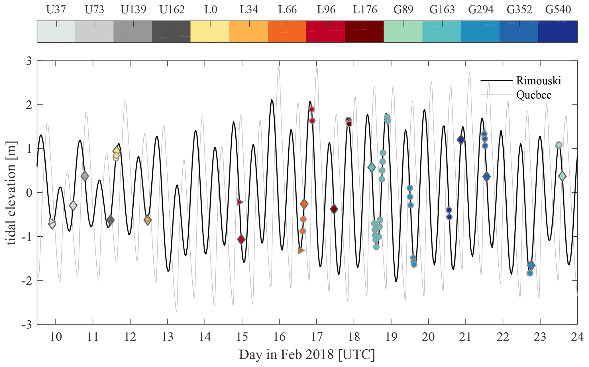
Figure 2 Observed tidal amplitudes at Rimouski (station no. 2985) and Quebec City (station no. 3248) maintained by Fisheries and Oceans Canada. The circles and diamonds respectively denote when the VMP and CTD rosette profiled at each station, designated by the color bar. The smaller triangle denotes the SBE 19 CTD, which provided near-surface measurements when the rosette was deployed from the moon pool. Tidal levels near station G163 (Grande-Vallée) precede those at Rimouski by about 15 min, while those recorded at Tadoussac (station L0) lag Rimouski by another 30 min.

2.2.2 Historical monitoring surveys

Fisheries and Oceans Canada run the Atlantic Zone Monitoring Program (AZMP) multiple times each year (Therriault et al., 1998; Blais et al., 2019; Galbraith et al., 2019). Their monitoring consists of surveys in March, June, August, and November, which cover the gulf and the lower estuary (Fig. 1a). Here, we present nitrate and salinities measured in summer and fall preceding our boreal winter campaign (Table 1). For completeness, we also present nitrate and salinity observations from the fall monitoring survey of the St. Lawrence Ecosystem Health Research and Observation Network. These nitrate samples were analyzed using the same procedures and equipment as those collected during the Odyssée 2018 winter field campaign.

The AZMP's ship-based fall and summer surveys provided standard CTD profiles, along with nutrient concentrations at depths similar to our winter campaign, in addition to samples closer to the surface at 2.5 and 5 m of depth. The summer nitrate measurements were collected from two different AZMP cruises (Table 1). The first cruise, during June, collected profiles in the downstream reaches of the upper estuary and near the HLC. The second cruise was in August and focused on the lower estuary and the gulf. Similarly to the Odyssée winter cruise, the nitrate concentrations were derived using colorimetric methods. The AZMP uses CSK standards from the Sagami Research Center, Japan, and participates in intercalibration exercises through the International Council for the Exploration of the Sea (Mitchell et al., 2002). From the CSK standards, the AZMP's nitrate concentrations have an accuracy (rms) of 3.1 %, 1.7 %, and 1.8 % at concentrations of 5, 10, and 30 µmol L⁻¹, respectively. The reported values represent the triplicate average. Their coefficients of variation were on average less than 1.2 %. The majority (95 %) of the 136 sets of triplicates had coefficients of variation below 3 %. The summer measurements are provided to contrast with our winter nutrient observations. We use the fall measurements to estimate the nitrate inventory generated between the fall monitoring survey and our winter observations within the lower estuary.

We also present observations from the winter heli-survey conducted in mid-March 2018, a few weeks after our winter program in February 2018 (Table 1). Like most years, the 2018 AZMP's winter survey was conducted by helicopter. Therefore, sampling was limited to CTD profiles (pumped Sea-Bird Scientific SBE 19plus V2). Surface water samples were also filtered, frozen, and analyzed later for nutrient concentrations. This campaign surveyed stations within the Saguenay Fjord in addition to the St. Lawrence in mid-March (Fig. 1b).

3 Data analysis

Our paper focuses on establishing the main transport pathways for nutrients in the lower estuary. In this region, nitrate concentrations are generally lower than silicate and therefore more likely to limit primary production (Tremblay et al., 1997; Jutras et al., 2020). Our subsequent analysis thus focuses on tracking nitrate inputs into the lower estuary's surface layer. We treat the upper 75 m of the lower estuary as a box. The box receives fluvial (horizontal) inputs of nitrate from the upper estuary and vertical inputs entering its base through mixing processes (Fig. 3a). These mixing processes include the intense tidal upwelling at the HLC and shear-induced mixing elsewhere in the lower estuary. Only mixing at the base of the box is considered, extending across the upper 75 m of the water column, since mixing within the box redistributes the fluvial nitrate entering from the upper estuary. Mixing at the box's base occurs at the interface between the different layers of water. The vertical mixing caused by the estuarine circulation is more persistent than tidal-dependent mixing at the head of the channel. The vertical nitrate fluxes will be quantified using the techniques described in Sect. 3.2 and applied to the respective surface areas of the HLC and the lower estuary. These vertical nitrate loads will then be compared to the horizontal fluvial inputs described in Sect. 4.3.1.

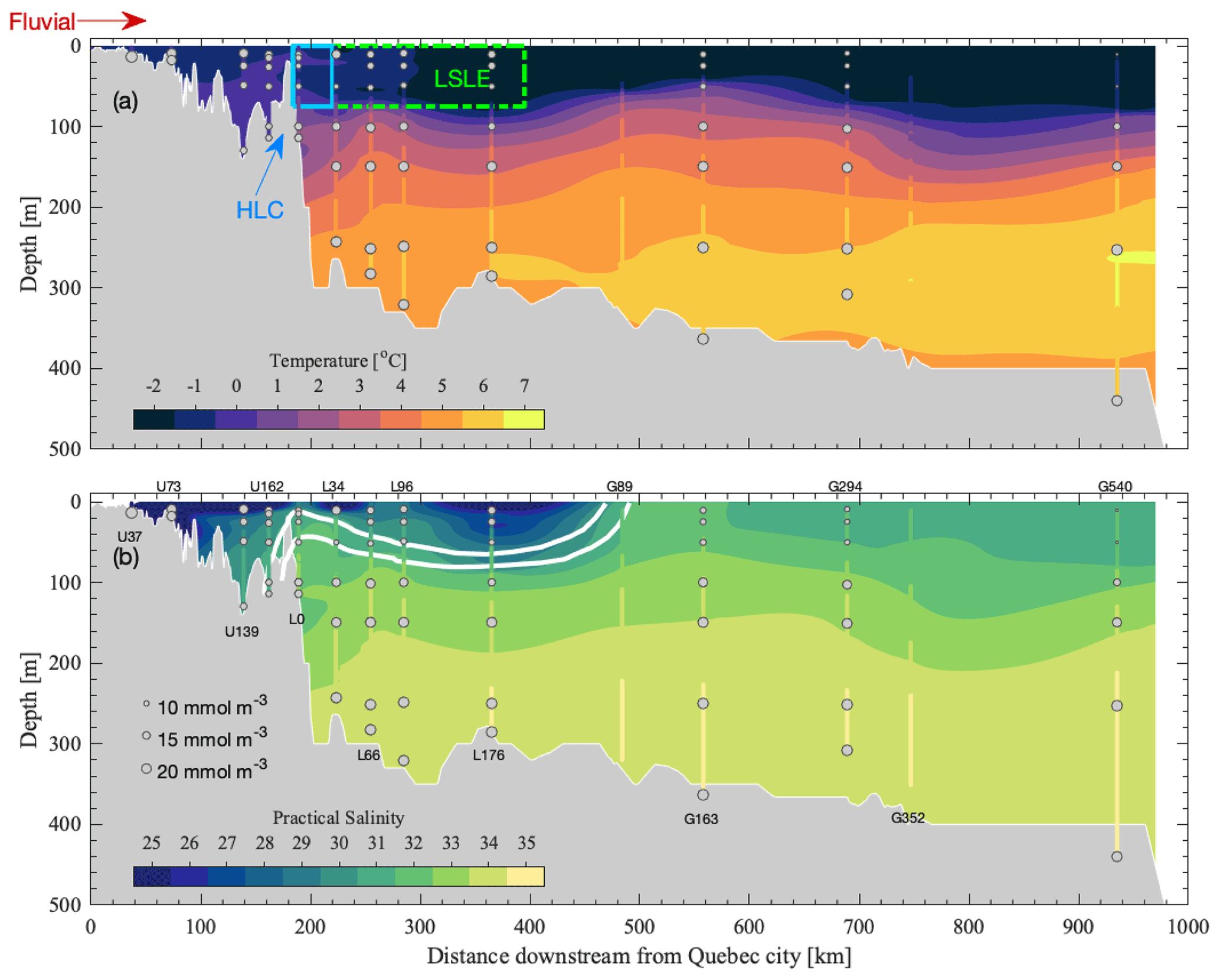
Figure 3 (a) Temperature and (b) salinity measured along the St. Lawrence during the winter field campaign. The gray circles are scaled with the nitrate concentrations of the rosette water samples in Fig. 4a. The extent of the HLC and the lower St. Lawrence Estuary (LSLE) is denoted in (a) by the cyan and green boxes, respectively. The thick white lines in (b) delineate the salinity limits of 31.2 and 31.9 used for developing the nitrate–salinity relationships (Eq. 4). Water above the upper line (S=31.2) originated from the upper estuary. Water below the lower line (S=31.9) originated from the gulf. The contours were obtained using a data-interpolating variational analysis (DIVA) technique (Troupin et al., 2012).

3.1 Fluvial nitrate loads

We estimated the advected (horizontal) fluvial contributions of nitrate into the lower estuary using nitrate concentrations and flow rates at Quebec City. The nitrate loads were thus calculated at the downstream extent of the upper estuary, where water is fresh. We assume that the fluvial loads in the lower estuary are representative of those at Quebec City or, alternatively, that our box includes the upper estuary. The fluvial nitrate loads, expressed in moles per second (mol s⁻¹), in the St. Lawrence River are calculated from

$$\begin{array}{}\text{(1)}& M_{\mathcal{N}}={\displaystyle \frac{Q\mathcal{N}}{\mathrm{1000}}}\end{array}$$

using the flow rate Q (m³ s⁻¹) and the nitrate concentration 𝒩 (mmol m⁻³) at Quebec City. These flow rates were calculated on a daily basis using the inverse modeling techniques recently developed by Bourgault and Matte (2020a, b). The approximate error in these daily and monthly flow rates is 0.25×10⁴ and 0.16×10⁴ m³ s⁻¹, respectively (Bourgault and Matte, 2020a). This method of estimating flows replaces the older and less accurate method of Bourgault and Koutitonsky (1999), which is currently issued on a monthly basis by the Government of Canada.

The historical dissolved nitrate–nitrite concentrations at Quebec City were digitized from published sources (Fig. 4 of Hudon et al., 2017). During our winter campaign, nitrite concentrations were 2 to 3 orders of magnitude less than nitrate concentrations. Our nitrate concentrations were thus representative of the sum of nitrate–nitrite concentrations presented by Hudon et al. (2017). Their measurements were collected every month and sometimes weekly from 1995 to 2011. We also estimated the fluvial nitrate loads during our winter campaign. The nitrate concentrations 𝒩 nearest Quebec City (station U37) were used in Eq. (1). The sampled water was almost fresh, with salinities below 0.5 and dissolved nitrate concentrations of 26.43 mmol m⁻³. The application of Eq. (1) to the historical measurements provided long-term statistics on the fluvial nitrate loads entering the upper estuary, which are presented in Sect. 4.3.1.

3.2 Turbulent vertical nitrate fluxes

We combined the VMP's turbulence profiles with the nutrient measurements to obtain vertical fluxes along the St. Lawrence during winter via

$$\begin{array}{}\text{(2)}& F_N\left(z\right)=-K\left(z\right){\displaystyle \frac{\partial \mathcal{N}\left(z\right)}{\partial z}},\end{array}$$

where z is the height above the free surface. The mixing rates K were derived from the VMP's measurements (Sect. 3.2.1), while the vertical background concentration gradients $\partial \mathcal{N}/\partial z$ were derived for nitrate from the VMP profiles via a nitrate–salinity relationship developed by analyzing the rosette's water samples (Sect. 3.2.2).

3.2.1 Diapycnal mixing rates K

The most commonly used model for estimating K was proposed by Osborn (1980) for shear-induced mixing,

$$\begin{array}{}\text{(3)}& K=\mathrm{\Gamma }{\displaystyle \frac{\mathit{ϵ}}{N^{\mathrm{2}}}},\end{array}$$

and requires estimating the rate of dissipation of turbulent kinetic energy ϵ and the background buoyancy frequency $N=\sqrt{(-g/\mathit{\rho })(\partial \mathit{\rho }/\partial z)}$. This last quantity depends on the vertical gradients of potential density ρ. A constant mixing efficiency Γ=0.2 is often assumed, despite mounting evidence that it varies (e.g., Monismith et al., 2018). Several parametric models have been proposed (e.g., Ivey et al., 2018), and debated (e.g., Gregg et al., 2018), to relate Γ with external parameters.

During the winter field program, the temperature gradients were generally gravitationally unstable, i.e., cold water overlaying warmer water. These unstable temperature gradients were stabilized by the salinity gradients. In these situations, double-diffusive convection (DDC) is possible. However, our observations lacked the presence of distinctive large (∼ several meters high) steps that are typically suggestive of DDC. Even when DDC dominates in weakly sheared flows, Eq. (3) can be used to estimate K by increasing Γ∼1 (see Hieronymus and Carpenter, 2016; Polyakov et al., 2019). In these situations, buoyancy is the main source of mixing. Our turbulence levels were much higher than those reported by Polyakov et al. (2019), and the strong tides are more conducive to shear-induced mixing than quiescent DDC mixing. We thus assume the custom value of Γ=0.2 for shear-induced mixing. Our chosen Γ is consistent with field observations at low $\mathit{ϵ}/\left(\mathit{\nu }{N}^{\mathrm{2}}\right)$ (e.g., Holleman et al., 2016; Monismith et al., 2018). Here, ν represents the kinematic viscosity of seawater, while the ratio $\mathit{ϵ}/\left(\mathit{\nu }{N}^{\mathrm{2}}\right)$ is proportional to the ratio of the largest and smallest turbulent overturns in a stratified fluid. During our field campaign, $\mathit{ϵ}/\left(\mathit{\nu }{N}^{\mathrm{2}}\right)$ was less than 500 95 % of the time.

To obtain the mixing rate K, we estimated ϵ using the methods described by Bluteau et al. (2016). Each profile was split into 4096 samples (8 s) that overlapped by 50 % before computing the velocity gradient spectra. The VMP's profiling speed was derived from its pressure sensor to convert the spectra between the frequency and wavenumber domain. We applied the multivariate technique of Goodman et al. (2006) to remove motion-induced contamination from these spectra, which were then integrated over the viscous subranges to obtain ϵ. The VMP typically profiled at around 0.65 m s⁻¹, thus providing turbulence estimates at a resolution of about 2.5 m given the 50 % overlap when splitting the cast. Turbulence estimates near the end and the beginning of a cast were discarded because of the VMP's deceleration and acceleration, respectively. We also discarded estimates within 25 m of the surface because of the turbulence induced by the ship. To derive the potential density gradients, we relied on the high-accuracy temperature and conductivity sensors (SBE 3F and SBE 4C) aboard the VMP. We first low-pass-filtered these signals with a Butterworth filter using a cutoff period of 8 s. We then centered-differenced these smoothed profiles before averaging them over the same segments used for getting ϵ, yielding the mean vertical gradients necessary for using Eqs. (2) and (3).

3.2.2 Proxy nitrate concentrations for estimating $\partial \mathcal{N}/\partial z$

Proxy nitrate concentrations are required to derive vertical nitrate gradients from the VMP's measurements (Eq. 2). This proxy made use of the winter dependency between nitrate and salinity. When limited amounts of nutrients are being consumed (or generated), mixing and advection processes govern the spatial distribution of nutrients. Their concentrations vary linearly with salinity, as reflected by our winter observations in Fig. 4f. A concave nitrate–salinity curve, such as observed during summer and fall 2017, indicated that biogeochemical processes caused a net loss of nitrate in the upper estuary (gray points in Fig. 4d and e). These trends in the nitrate–salinity diagrams are supported by incubation experiments that quantify the nitrate uptake (Villeneuve, 2020). Nitrate uptake in the lower reaches of the upper estuary and in the lower estuary was almost an order of magnitude higher in summer than during winter. Nitrate uptake downstream of Quebec City was less than 0.50 nmol m⁻³ s⁻¹ and about half as much in the lower estuary (Fig. 16 of Villeneuve, 2020). Hence, a nitrate–salinity relationship is thus justified to estimate nitrate from the VMP's salinity measurements during winter.

Nitrate concentrations in winter depended on salinity but also on the location in the St. Lawrence (Fig. 4). The nitrate variations are associated with the water masses in the region. The temperature–salinity diagram suggests two, possibly three, significant water masses across the region (Fig. 4a). The first water mass is composed of nutrient-rich waters from the upper estuary that mix in the lower estuary before eventually mixing with nutrient-poor surface water downstream in the gulf (Fig. 4d). This mixing resulted in nitrate 𝒩 concentrations decreasing with salinity for S<31.2. For higher salinities, S>31.9, which includes samples deeper than 50 m in the lower estuary and almost all samples in the gulf, nitrate increased proportionally with salinity (Fig. 4f). This vertical nutrient distribution resembles the expected waters exposed to the open ocean, which we associate with the region's second water mass. Evidence of a third water mass is featured between 31.2 and 31.9 for nitrate, phosphate, silicate, and, in particular, the temperature–salinity diagram of lower estuary stations (Fig. 4). The salinity of 31.2 corresponds to a local subsurface maximum in water temperatures at station L0, where the Saguenay Fjord enters the St. Lawrence, and downstream at L34. The heli-survey a month later confirms that the Saguenay Fjord discharged fresher water near this station (Fig. 4a). The surface water samples at the head of the Fjord had much lower phosphate (∼0.2 mmol m⁻³) and nitrate (∼10 mmol m⁻³) than water with comparable salinity in the upper estuary (Fig. 4). This third water mass created a more rapid decrease in nitrate between the 31.2 and 31.9 salinity range before increasing again due to mixing with gulf waters within the lower estuary (Fig. 4f).

From the observed water masses in winter, we created three separate nitrate–salinity relationships to obtain proxy nutrient concentrations from the VMP's salinity measurements:

$$\begin{array}{}\text{(4)}& \mathcal{N}\left[\mathrm{mmol}{\mathrm{m}}^{-\mathrm{3}}\right]=\left\{\begin{array}{l}-\mathrm{0.70}S+\mathrm{34.9}\\ \text{for }S\le \mathrm{31.2},\\ -\mathrm{4.37}{S}^{\mathrm{2}}+\mathrm{272.3}S-\mathrm{4230}\\ \text{for }\mathrm{31.2}<S\le \mathrm{31.9},\\ \mathrm{4.84}S-\mathrm{144.2}\\ \text{for }S>\mathrm{31.9}\text{ or in the gulf.}\end{array}\right.\end{array}$$

The first relationship, applicable for S<31.2, reflects the nutrient-rich water in the upper estuary mingling with saltier water downstream. The third relationship included all samples with S>31.9. It was applied to turbulence profiles within the gulf except for the deep data near Cabot Strait (station G540, ≳250 m). These data correspond to a fourth water mass, which we exclude from our vertical nitrate flux analysis. The second relationship links the other two using a quadratic fit to the samples outside the gulf within the range $\mathrm{31.2}<S\le \mathrm{31.9}$. This relation reflects contributions from the Saguenay Fjord, which was applied solely to turbulence profiles collected in the lower estuary. Outside the $\mathrm{31.2}<S\le \mathrm{31.9}$ range, we applied the first or third relationship over their applicable salinity ranges. Typically, the first relationship was applied to surface waters in the lower estuary that originated from the nutrient-rich upper estuary upstream. In contrast, the third relationship was used for deeper waters entering from the gulf. A mean relative error of 5.5 % was obtained for the predicted 𝒩 after applying Eq. (4) to all 64 samples in Fig. 4f. The poorest agreement is with the low surface nitrate concentrations measured in the gulf, particularly the furthest downstream near Cabot Strait (station G540 in Fig. 4f). The proxy nitrate concentrations calculated from Eq. (4) were then used to estimate the vertical nitrate gradients for obtaining vertical fluxes from Eq. (2).

3.2.3 Vertical mixing contributions of nitrate

To convert the vertical nitrate fluxes into mass loadings, we rely on the same techniques as Cyr et al. (2015) to determine the tidal upwelling zone. The intense mixing creates a surface signature of cooler water during summer (see Fig. 13 of Cyr et al., 2015) and likely coincides with the winter polynya observed during regular monitoring (see Fig. 10 of Galbraith et al., 2019) and our winter cruise (Fig. 4a). Their estimated surface area was approximately 100 to 200 km². For our box analysis, we require the surface area at the 75 m isobath rather than at the air–sea interface. At this isobath, the entire lower estuary covers about 6000 km², whereas the head of the channel is about 200 km² (Fig. 3a). This area is larger than the 100 km² used by Cyr et al. (2015). We thus exaggerate the impact of the HLC on transporting nitrate into the surface layer by using the area upper bound of 200 km². For the remaining 97 % of the lower estuary's area, we apply the average vertical nitrate fluxes obtained outside the HLC to the base of our box.

Figure 4 Winter 2018 observations of (a) potential temperature (at atmospheric pressure), (b) phosphate, and (c) silicate illustrated against salinity. The nitrate concentrations for (d) the summer 2017, (e) fall 2017, and (f) winter 2018 are also shown. The symbols in panels (b)–(f) indicate the sample's depth. The open diamonds are near the surface (depth <20 m), while the closed triangles and squares are samples at 25 and 50 m, respectively. The closed circles represent deeper samples at or below 100 m. The two vertical dotted lines in (f) denote salinities of 31.2 and 31.9. Density contours in σ_T [kg m⁻³] (a) were computed at atmospheric pressure. Concentrations measured from the most upstream station U37 were 26.43 mmol m⁻³ for nitrate, 0.53 mmol m⁻³ for phosphate, and 39.8 mmol m⁻³ for silicate. This bottle at 10 m of depth corresponded to salinity of ≈0.5. T_f is the freezing temperature of seawater in (a).

4 Results

4.1 Winter conditions

We visited the head of the channel during an upwelling event (Fig. 3b). The salinity was relatively homogeneous across the depth when we sampled at L0 during the flooding tide (Fig. 2). The water was nonetheless 2 units more saline than near-surface waters (i.e., 15 m) measured at stations both upstream and downstream from the head of the channel (Fig. 3b). The higher salinities at the head of the channel, station L0, cannot be attributed to inputs from the Saguenay Fjord. This waterway provides a freshwater source, confirmed by the AZMP's annual helicopter survey a few weeks later (Fig. 4a). We attribute the relatively high salinities around the HLC to tidal upwelling and mixing that characterize this region throughout the year (Ingram, 1983; Galbraith, 2006; Cyr et al., 2015). At the HLC, nitrate concentrations in the upper 50 m were also lower than water both upstream and downstream at comparable depths (Fig. 3a). This low-nitrate and high-salinity water, especially in the upper 50 m, further supports the fact that water was tidally upwelled.

The transects illustrate the presence of a subsurface nitrate minimum in the lower estuary (Fig. 5b). During winter, nitrate concentrations were relatively high near the surface. Concentrations decreased to reach a subsurface minimum at the 50 m deep sample. These subsurface samples were near or slightly more saline than 31.2, which is the corresponding break between nutrient-rich fluvial waters and the relatively nutrient-poor water downstream seen in the nitrate–salinity diagram (Fig. 4f). In the lower estuary, a nitrate-poor subsurface layer is overlaid by fresher and nitrate-rich surface waters.

4.2 Seasonal nitrate variations

We observed this nitrate-poor subsurface layer during other seasons (Fig. 5b–d). Climatological averages show that a subsurface nitrate minimum is typical of the lower estuary's lower reaches during the ice-free months (see Fig. 3 of Cyr et al., 2015). Above this layer, near-surface nitrate concentrations are higher, especially during winter (e.g., ∼ 350 km in Fig. 5b). These high nitrate concentrations were associated with low salinities (e.g., station L34 and L176 in Fig. 4), reflecting the input of nutrient-rich fluvial water from the upper estuary. During winter, these fluvial waters likely extended downstream to 400 km from Quebec City (station L176; Fig. 5b) but extended less far in the fall (300 km, Fig. 5c). The subsurface nitrate minimum created by the fluvial waters in the lower estuary was more evident during winter and fall than in summer because of the higher biological uptake during summer (200–300 km, Fig. 5d). However, the nitrate–salinity diagrams show that fluvial waters may be perceptible just as far downstream into the lower estuary during summer as in fall (Fig. 4d-e). Upstream in the upper estuary, nitrate concentrations were highest in winter, followed by the fall and summer (Fig. 5b-d). Overall, the upper estuary supplied nitrate-rich fluvial waters into the surface layer of the lower estuary.

Figure 5 (a) Nutrient inventory generated in the upper 75 m of the lower estuary's water column. (b) Nitrate concentrations during our winter field campaign, (c) fall 2017, and (d) summer 2017 monitoring surveys. The thick cyan lines in (b) denote the same water masses as in Fig. 3. Water between these two lines coincides with the subsurface nitrate minimum at station L0 and downstream. The gray circles are scaled with the salinity of the water samples as shown in Fig. 4. The contours were obtained using a data-interpolating variational analysis (DIVA) technique (Troupin et al., 2012).

The nutrient inventory created in the upper 75 m of the lower estuary during the fall and winter measurements is illustrated in Fig. 5a. The inventory is obtained by depth-integrating the difference between the fall and winter measurements (Fig. 5b and c). This analysis assumes no nitrate uptake between these two seasons, i.e., no sink term. For completeness, we also added the inventory created between winter and summer, which is about 25 % larger than the nitrate that accumulated between winter and fall. Hence, most of the nitrate accumulated in the surface layer between fall and winter because of the high nitrate uptake during summer (Fig. 16 of Villeneuve, 2020). The lower estuary's inventory mainly includes contributions from the nitrate-rich and fresher water originating from the upper estuary (i.e., S<31.2 in Fig. 4). The high values at 420 km reflect the nitrate-rich and fresher water from the upper estuary during winter. The near-surface nitrate is relatively depleted during fall at this location (Fig. 5a–b). The spatially averaged inventory for the lower estuary between fall and winter was 280 mmol m⁻², which translates to an equivalent vertical flux of 32 nmol m⁻² s⁻¹ given the 100 d between these measurements. Hence, during this period, nitrate in the upper 75 m of the lower estuary increased by about 195 mol s⁻¹. Repeating a similar calculation for the period between summer and fall yields a nitrate accumulation rate of roughly 95 mol s⁻¹, which is about half as much as the period between fall and winter.

4.3 Nitrate transport pathways

We now present the annual cycle of fluvial nitrate loads compared with the vertical loads entering the lower estuary from vertical mixing processes.

4.3.1 Fluvial nitrate loads

The fluvial nitrate loads vary seasonally, reflecting the changes in dissolved nitrate concentrations and flow rates at Quebec City. The 17-year-long statistical records show that nitrate concentrations reach their annual minimum of ∼14 mmol m⁻³ at the end of summer (August and September, Fig. 6a). Nitrate concentrations progressively increase during fall and remain relatively steady between December and March. Nitrate uptake is weakest during the winter months (Villeneuve, 2020). In spring, nitrate concentrations increase, which peaks at ∼32 mmol m⁻³ in May before steadily decreasing throughout the summer period. Flow rates follow a similar pattern, although the snowmelt generates a more pronounced increase during spring. Flows peak in April with the average exceeding 16×10³ m³ s⁻¹, whereas they reach minimum annual values in late summer with average flow rates below 10×10³ m³ s⁻¹ (Fig. 6a). During our 2018 winter campaign, the flow rates were relatively large compared to the long-term historical averages for February. However, our measured nitrate concentrations were similar to the February average.

Our observed flows and nitrate concentrations in February 2018 translate into a fluvial nitrate input of 350±65 mol s⁻¹ at Quebec City. This value is slightly higher than the 17-year average for February and also higher than the historical average of 300±20 mol s⁻¹ for the winter months of November through February (Fig. 6b). The fluvial nitrate loads peaked in April when the historical averages reached 500 mol s⁻¹ before decreasing to their annual minimum in August and September. During these late summer months, nitrate loads are below 150 mol s⁻¹ (Fig. 6b). These low nitrate loads coincide with the period when biological uptake is greatest upstream of Quebec City (Hudon et al., 2017) and flow rates are at their lowest. The fluvial inputs during the field experiment of Cyr et al. (2015) were about 90 mol s⁻¹, which is much lower than historical averages (Fig. 6b). Their fluvial nitrate loads were more than 3 times less than those during our winter campaign.

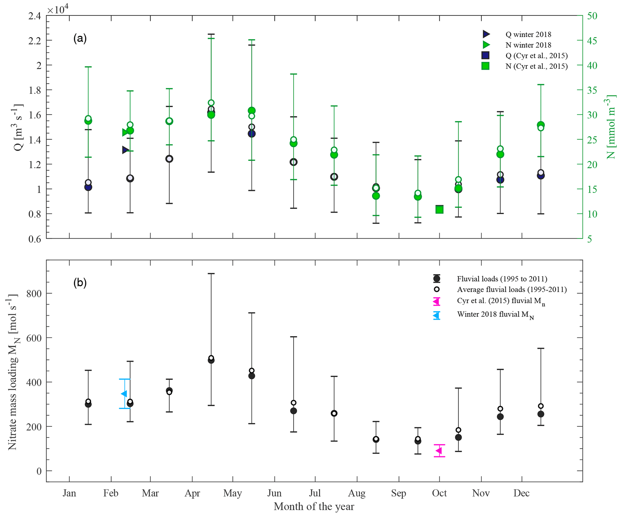
Figure 6 (a) Monthly statistics of the freshwater flow rates at Quebec City from 1995 to 2011 using the inverse modeling techniques described by Bourgault and Matte (2020a). The secondary green axis represents the monthly statistics of nitrate concentrations measured at Quebec City during this same period (Hudon et al., 2017). (b) Monthly statistics of the mass nitrate fluvial loads estimated from Eq. (1). The bars in both panels extend from the 5th and 95th percentile for each month's data and are centered around the median (dark circles). The open circles denote the monthly averages. The error bars on the instantaneous nitrate loads for our winter 2018 campaign and Cyr et al. (2015) late summer observations are the errors propagated from the flow estimates. The nitrate concentrations for Cyr et al. (2015) were interpolated from the temporal time series of Hudon et al. (2017) at Quebec City.

4.3.2 Turbulence observations and vertical nitrate fluxes

The vertical nitrate fluxes were determined from the direct turbulence measurements along the lower St. Lawrence Estuary and the Gulf of St. Lawrence (Fig. 7). The turbulence observations were most energetic in the upwelling-driven polynya near the head of the channel. At station L0, at the sill near the head, dissipation ϵ exceeded 10⁻⁷ W kg⁻¹ near the bottom and the surface (Fig. 7a), while the mixing rates K exceeded 10⁻⁴ m² s⁻¹ throughout most of the water column (below 60 m and above 30 m of depth, Fig. 7b). The other stations were relatively quiescent with ϵ of the order of 10⁻⁹ W kg⁻¹. Elevated diapycnal mixing rates were also found in the surface mixed layer (depth <50 m), especially in the gulf. These high rates are presumably due to winter convective mixing processes reaching the deeper pycnocline (Fig. 7d). Elsewhere in the water column, outside the energetic HLC, mixing rates were more typical of the ocean interior (𝒪(10⁻⁵) m² s⁻¹; Waterhouse et al., 2014). Near the HLC, our winter “hot spot”, diapycnal mixing estimates were within the ranges observed during the summer months (e.g., Fig. 11 of Cyr et al., 2015). Our winter fluxes would have likely been higher if collected later at high tide, as shown with the late summer observations of Cyr et al. (2015). They measured $K\approx {\mathrm{10}}^{-\mathrm{2}}$ m² s⁻¹ at high tide between depths of 25 and 50 m compared to $K\approx {\mathrm{10}}^{-\mathrm{4}}$–10⁻³ m² s⁻¹ about 2 h earlier. High mixing occurred at the HLC and at the base of the surface layer elsewhere in the system.

Figure 7 (a) ϵ, (b) K, and (c) F_𝒩 after time-averaging the repeated VMP profiles at each station. We present the average profiles for the lower estuary (outside the HLC) and in the gulf for (d) ϵ, (e) K, and (f) F_𝒩. The error bands represent 95 % confidence intervals obtained through bootstrap analysis on the averages within each region. The HLC's vertical fluxes in (f) are shown on a separate axis. The gray contour lines in (a) and (b) represent isopycnals (in σ_T, kg m⁻³), whereas those in (c) are the nutrient contours (in mmol m⁻³) shown in Fig. 5b. Positive values in (c) indicate an upward flux of nutrients. The thick cyan lines in (c) are the same as in Fig. 3 – the 31.2 and 31.9 isohalines that delineate water originating from the upper estuary (S<31.2) and from the gulf (S>31.9). The contour lines were obtained using a data-interpolating variational analysis (DIVA) technique (Troupin et al., 2012).

We obtained the largest vertical fluxes of nitrate near the head of the channel, where mixing was highest. Nitrate fluxes F_𝒩 were particularly elevated in the deeper part of the water column where they exceeded 30 nmol m⁻² s⁻¹ below 80 m (Fig. 7c). This flux converts into a vertical supply of nitrate of about 6 mol s⁻¹ into the surface layer over the exaggerated surface area of 200 km² for the HLC (Sect. 3.2.3). Further downstream in the lower estuary, nitrate fluxes were lower than at the head of the channel. Vertical nitrate fluxes were generally higher at the interface, separating the subsurface nitrate minimum from water below it. The fluxes dropped in magnitude further downstream in the lower estuary (station L66 vs. L176 at 60 m of depth, Fig. 7c). Vertical nitrate fluxes were much weaker in the gulf than in the lower estuary, with weak upward fluxes at the surface layer's base. Occasional storms would increase surface mixing, but its effects would unlikely be felt below 75 m in the lower estuary given the stratification imparted by the fluvial waters. Storms, instead, would tend to mix down the nutrient-rich surface water of fluvial origin into the relatively nutrient-poor water beneath it.

In the lower estuary, nutrients were transported by turbulence mixing processes upwards and downwards into the subsurface minima. On average, the nitrate-rich surface waters from the upper estuary were mixed downwards at 4.8 nmol m⁻² s⁻¹ into this nitrate-poor subsurface layer in the lower estuary (50 m of depth, Fig. 7f). The nutrient-rich water, originating from the gulf, was mixed upwards into this subsurface layer at a lower rate of 2.4 nmol m⁻² s⁻¹ (≈80 m of depth, Fig. 7f). These elevated upward fluxes at this depth coincide with the nitricline beneath the subsurface nitrate minima. The nitricline sits at the 26.5 kg m⁻³ isopycnal, which is 80±5 m deep at the stations downstream of the head in the lower estuary (Fig. 7b and c). Only the vertical nitrate fluxes from below the subsurface layer contribute to the lower estuary surface layer's overall supply. When converted into a vertical nitrate load, the relatively weak vertical fluxes outside HLC supplied 14 mol s⁻¹ into the lower estuary's surface layer. If we add the contributions at the HLC, the total vertical nitrate load into this layer was of the order of 20 mol s⁻¹ during our winter campaign.

We now explore the possibility that our vertical nitrate loads measured during winter may underestimate the actual nitrate contributions given the tidal variability of the mixing at the head of the channel. For this analysis, we rely on the tidally resolved summer measurements of Cyr et al. (2015), which are reproduced in Fig. 8 with our winter vertical fluxes. Our winter flux estimate at the head was consistent with theirs collected at the same tidal phase, i.e., 2 h before high tide (Fig. 8a). However, their summer mixing and vertical nitrate fluxes increased by almost 3 orders of magnitude during the semi-diurnal tidal cycle, with fluxes peaking at high tide. We converted their vertical fluxes into nitrate loads supplied across the head's area in Fig. 8b. Their averaged value of ∼1 $\mathrm{\mu }\mathrm{mol}{\mathrm{m}}^{-\mathrm{2}}{\mathrm{s}}^{-\mathrm{1}}$ results in a vertical nitrate load of about 210 mol s⁻¹. This estimate likely overexaggerates the vertical contributions from mixing processes at the head since removing the highest estimate reduces the average nitrate flux by 50 %, yielding an equivalent vertical load of 100 mol s⁻¹. Their median estimate is even lower than this average, reducing the vertical nitrate load to 25 mol s⁻¹ for the head of the channel (Fig. 8b). All these estimates of the vertical nitrate loads are still lower than the fluvial loads of 350 mol s⁻¹ entering the lower estuary during winter.

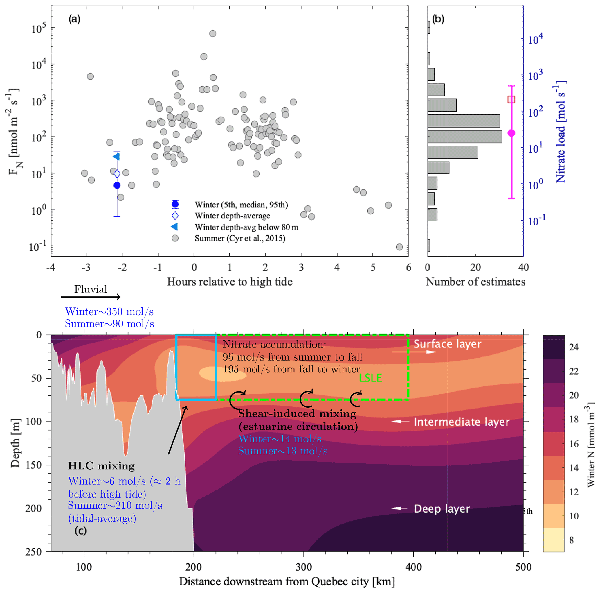
Figure 8 (a) Nitrate fluxes at the HLC as a function of the tidal phase for winter and summer. The summer estimates from Cyr et al. (2015) are re-illustrated in (b) as a histogram. The error bar shows the 5th and 95th percentile of the observations and is centered around the median F_𝒩 (blue is winter and magenta is summer). (c) Close-up of Fig. 5b with the estimated nitrate loads from vertical mixing and fluvial contributions. The cyan and green box denotes the extent of the HLC and lower estuary, respectively. The secondary y axis in (b) is the vertical nitrate load after multiplying F_𝒩 by the surface area of 200 km². The contours were obtained using a data-interpolating variational analysis (DIVA) technique (Troupin et al., 2012).

5 Discussion

We revisit the notion of mixing processes, especially tidal-induced mixing at the head of the channel, acting as the nutrient pump for the lower estuary. The low uptake during winter better represents the physical mechanisms transporting nitrate into the lower estuary than in summer. Summer observations invariably track both physical and biological processes. Studies have reached variable conclusions about the importance of tidal mixing at the HLC in supplying nutrients to the lower estuary and ultimately the gulf (see Sect. 1). All of these studies concluded that vertical mixing processes dominate the supply of nutrients in the lower estuary (e.g., Steven, 1974; Sinclair et al., 1976; Savenkoff et al., 2001; Cyr et al., 2015; Jutras et al., 2020; Greisman and Ingram, 1977). The biogeochemical box model of Jutras et al. (2020) predicted vertical nitrate loads of 1050 mol s⁻¹ for the entire lower estuary, while that of Savenkoff et al. (2001) predicted 685 mol s⁻¹. To reach these high values, the turbulent nitrate fluxes at the HLC would need to be 2 to 4 times larger than the summer values observed by Cyr et al. (2015), yet their summer fluxes were some of the highest reported in the world (Fig. 5 of Mouriño-Carballido et al., 2021).

These biogeochemical studies contrast with our winter observations since the fluvial nitrate loads dominated the supply of nutrients into the lower estuary (Fig. 8c). Our conclusion remains true even if the winter vertical nitrate fluxes at the HLC reached values as high as those measured during summer upwelling. During winter, the lower estuary's intermediate layer coincides with our observed nitrate subsurface minima. So the estuarine circulation entrains nitrate-rich fluvial waters into the nitrate-poor subsurface layer (Fig. 8c). Our direct turbulence observations indicate that the estuarine circulation in the lower estuary causes relatively weak entrainment of deep bottom waters into the intermediate layer. The vertical nitrate load caused by this entrainment was about 14 mol s⁻¹ – the same magnitude as that obtained by Cyr et al. (2015) during late summer (Fig. 8c). The nitrate–salinity diagram (Fig. 4a) and their transects (Fig. 5) also highlight the fact that a large portion of the nitrate in the lower estuary originates from fluvial sources entering from the upper estuary.

Our results indicate that the fluvial loads are a much more significant input of nutrients into the lower estuary than turbulence mixing processes and are transported far into the lower estuary. Previous studies have been biased by the dynamics at the end of summer or may have been too limited in spatial coverage to track the fluvial nitrate-rich waters into the lower estuary. For example, Cyr et al. (2015) focused on the importance of vertical mixing in supplying nutrients into the lower estuary's euphotic zone. Although some of the world's largest, their vertical nitrate fluxes exceed fluvial inputs only during their measurement period – late summer to early fall. This period is when the fluvial nitrate loads reach their annual minimum (Fig. 6b). In fact, they collected their measurements of vertical fluxes when fluvial loads reached historical lows (Fig. 6b). Their average vertical load of nitrate (210 mol s⁻¹), for which we exaggerated the area of influence of tidal mixing processes at the HLC, exceeds fluvial loads only during summer from August to October (Fig. 6b). Thus, vertical mixing processes become an important source of nitrate into the euphotic zone of the lower estuary, mainly during summer. This observation is typical for temperate coastal and shelf waters during summer when the surface layer's temperature stratification is strongest (e.g., Bendtsen and Richardson, 2018; Mouriño-Carballido et al., 2021).

Future field campaigns should focus on documenting the physical processes responsible for upwelling nitrate into the euphotic zone at the head of the channel, specifically estimating the magnitude of the vertical nitrate fluxes during an entire semi-diurnal tidal cycle for both neap and spring tides. Peak tides could pump nitrate into the surface layer at a much higher rate, as shown by Cyr et al. (2015). Differences in magnitude could exist between neap and spring tides (e.g., Sharples et al., 2007; Green et al., 2019). The goal of these additional measurements would be to remedy the the short portion of the tidal cycle resolved during winter. Our winter observations were nonetheless consistent with the tidally resolved measurements of Cyr et al. (2015) during summer.

6 Conclusions

The inaugural Odyssée campaign aboard the CCGS Amundsen icebreaker provided the first winter turbulence measurements in the St. Lawrence Estuary and the Gulf of St. Lawrence. We collected these measurements in tandem with the vessel's ice-breaking and ship escorting operations. These mixing measurements covered the most considerable spatial extent of the estuary and gulf during any season. Our analysis shows that tidal-induced mixing appears to be a less effective mechanism for supplying nutrients in the euphotic winter zone than in summer. In fact, for most of the year, we expect higher nitrate loads from fluvial sources than from vertical mixing processes, in particular during freshet as the snowpack melts. At this time of the year, both nitrate concentrations and flow rates are highest (Fig. 6). The fluvial nutrient loads during winter, when biological uptake is low, likely precondition the phytoplankton spring bloom far into the lower estuary and adjacent gulf. Throughout most of the year, the fluvial contributions from the urbanized catchment upstream of Quebec City are a vital nutrient supply to the St. Lawrence Estuary.