Sea surface salinity short-term variability in the tropics

Using data from the Global Tropical Moored Buoy Array, we study the validation process for satellite measurement of sea surface salinity (SSS). We compute short-term variability (STV) of SSS, variability on timescales of 2–17 d. It is a proxy for subfootprint variability over a 100 km footprint as seen by a satellite measuring SSS. We also compute representation error, which is meant to mimic the SSS satellite validation process where footprint averages are compared to pointwise in situ values. We present maps of these quantities over the tropical array. We also look at seasonality in the variability of SSS and find which months have maximum and minimum amounts. STV is driven at least partly by rainfall. Moorings exhibit larger STV during rainy periods than during non-rainy ones. The same computations are also done using output from a high-resolution global ocean model to see how it might be used to study the validation process. The model gives good estimates of STV, in line with the moorings, although tending to have smaller values.

1 Introduction

Sea surface salinity (SSS) has been measured by satellites for more than a decade. Along the way there have been remarkable advances in the quality of the data and their applications (Reul et al., 2020; Vinogradova et al., 2019). SSS is measured by satellites using L-band radiometers, combined with ancillary measurement of sea surface temperature (SST), sea ice, rain rate, and wind speed as well as corrections for factors such as galactic radiation, Faraday rotation in the atmosphere, and radio frequency interference (Meissner et al., 2018; Olmedo et al., 2021).

As the database of satellite-based SSS measurements grows, the need to fully document the errors in the measurements becomes more acute. Many of the sources of error are well known and quantified (Lagerloef et al., 2008; Meissner et al., 2018); however, an important source has not been as well studied, that of representation error (RE). The accuracy of SSS measurements is often assessed by comparison with individual in situ readings, such as might be taken by an Argo float (e.g., Abe and Ebuchi, 2014; Kao et al., 2018b; Olmedo et al., 2017; Dinnat et al., 2019), mooring, glider, or ship, a process known as validation. RE is when two measurements being compared do not represent the same quantity. That is, the validation measurement and the satellite measurement are mismatched somehow in scale or timing. In the case of comparisons with float measurements, there may be differences between satellite and validation measurement not due to error or inaccuracy in in situ instruments nor to retrieval, but to a mismatch in scale between the two systems. One example of RE is that of subfootprint variability (SFV; Boutin et al., 2016; Bingham, 2019). SFV occurs because the SSS satellite measurement is made over a large footprint, whereas individual float measurements are made at a single point. The footprint of the satellite is 100 km in the case of the Aquarius satellite (Lagerloef et al., 2008) and ∼ 40 km in the case of the Soil Moisture Active Passive (SMAP) satellite (Meissner et al., 2019). The other major SSS satellite, SMOS (Soil Moisture and Ocean Salinity), does not have a simple footprint due to its interferometric method of sensing and wide field of view, but ranges from 35 to 63 km depending mostly on the viewing angle relative to nadir (González-Haro, personal communication 2021).

SFV has been discussed in detail by Bingham (2019). That paper quantified SFV for a 100 km satellite footprint at two locations, the SPURS-1 (Salinity processes in the Upper-ocean Regional Studies-1) region in the subtropical North Atlantic and the SPURS-2 region in the eastern tropical North Pacific, using a combination of drifter salinity, thermosalinograph, and wave glider data. The paper computed not just SFV but also its impact on satellite SSS error at those two locations. The analysis was further extended to include a variable footprint size by Bingham and Li (2020). One clear result of these two efforts is the difference between the two regions, and the time variability of SFV. The SPURS-2 region has a higher amount of SFV than SPURS-1, less dependence on footprint size, and less seasonal variability. This difference may have been due to the influence of differences in rainfall and/or internal ocean variability at the two sites. The analysis of Bingham (2019) also included a comparison of SFV computed from in situ data with short-term variability (STV) computed from moorings located at the two sites. The two were similar in magnitude and had similar seasonality, indicating that STV from a mooring could be used as a reasonable proxy for SFV from distributed in situ data. In this paper, we take that conclusion and go further with it. We make use of data from the Global Tropical Moored Buoy Array (GTMBA) to compute STV as a proxy for SFV over the global tropics and quantify SSS SFV, RE, and their magnitude, variability, and geographic distribution.

Another type of RE that is commonly thought of is temporal aliasing. SSS satellites have a limited footprint extent and limited temporal coverage. In the case of Aquarius, the satellite repeated every 7 d, whereas SMAP repeated every 2–3 d (Reul et al., 2020). Thus, an in situ measurement may not be simultaneous with a satellite overpass in time, leading to a potential difference between the two or resulting in temporal aliasing. In this paper, due to our use of temporal sampling as a proxy for spatial sampling, we cannot distinguish between SFV (or spatial aliasing) and temporal aliasing. However, we will briefly discuss the temporal aliasing issue.

SSS data from the GTMBA have been used in the past for comparison with satellites. Most comparisons have been done at Level 3 (L3; Bao et al., 2019; Tang et al., 2017; Qin et al., 2020; Tang et al., 2014), although some have been done at Level 2 (L2; Abe and Ebuchi, 2014; Kao et al., 2018a, b; Tang et al., 2014). For example, Bao et al. (2019) computed root-mean-square (RMS) differences and bias between mooring, satellite (SMOS and SMAP), and in situ gridded (EN4; Good et al., 2013) data, where the mooring data used were 8 d moving averages. Tang et al. (2017) computed similar statistical comparisons between moorings and SMAP, again using 8 d average values. Qin et al. (2020) reported the RMS error and bias between satellite SSS and a small set of moorings. While the GTMBA moorings have been a useful point of comparison for validation, as indicated by the number of studies we have just cited, they have not (to date) been used to study the process by which validation is carried out. As the mooring data are generally high quality, sampled at a high frequency, dispersed broadly over a diverse set of tropical regimes, and are placed very near the surface, they make an ideal platform for this.

One complementary aspect that we will study here is the use of high-resolution model output for exploring STV. Bingham (2019) and Bingham and Li (2020) both compared SFV from a high-resolution model (different from the one we will use here) and from in situ data and found that the two agreed reasonably well, especially in the subtropical SPURS-1 region. We would like to use such model output to study SFV on a global scale. The comparison of statistics from the moorings and the global model can give us confidence that model output may be used for this purpose.

2 Data and methods

We use two sources of in situ data: velocity data from the OSCAR (Ocean Surface Current Analysis Real-time) dataset, and SSS and rainfall from the GTMBA. We will also use data from the MITgcm (Massachusetts Institute of Technology general circulation model) as described below.

In this paper, we use practical salinity from the 1978 practical salinity scale. This scale is unitless; thus, following Millero (1993), we do not use the terms “psu” or “pss” as a substitute for units.

2.1 GTMBA SSS

The GTMBA is a vast network of buoys stretching across the global tropics (Fig. 1). It was originally set up in the mid-1980s to measure El Niño-related variability in the tropical Pacific (McPhaden et al., 1998, 2010) and has since been expanded to the Atlantic (Foltz et al., 2019) and Indian (McPhaden et al., 2009) basins. The moorings have sensors that measure SSS at ∼ 1 m depth with a Sea-Bird SBE 37 MicroCAT instrument (Freitag et al., 2018). GTMBA SSS measurements are reported hourly. No quality control was carried out beyond that done by the agencies operating the array. Bao et al. (2019) identified a small number of moorings with suspicious drifts in their SSS records. We examined the same records and did not judge them to be problematic. As the analysis done here uses short bursts of data to study variability, usually on timescales of ∼ 7 d or less, the absolute accuracy of the sensor is not crucial. SSS in the tropics tends to be quite spiky, with many low outliers, (e.g., Bingham et al., 2021a, their Fig. 2). Overly stringent quality control could eliminate many valid data points and alter the statistics of the record.

Figure 1 The small black dots represent GTMBA mooring locations. The red lines represent the mean OSCAR current speed over the 1992–2020 time period at each mooring location. Line lengths indicate the average speed, with a scale in blue (top center). The length of the scale corresponds to 25 cm s⁻¹. At that speed, it takes 4.6 d to travel 100 km. Thus, the line length also corresponds to the time span used in the computation of short-term variability discussed in the text. A shorter line (slower speed) means a longer time span. The directions of the lines have no meaning. Panel (a) shows the Pacific Basin, and panel (b) shows the Atlantic and Indian basins.

Many of the GTMBA moorings also recorded precipitation using an R. M. Young 50203 self-siphoning rain gauge (Freitag et al., 2018). The available records are at 1 min intervals, from which we computed hourly averages.

2.2 OSCAR currents

Ideally, in order to determine SFV, we would have a spatially distributed set of ocean measurements taken simultaneously, like those from SPURS-1 and 2 (Bingham, 2019; Bingham and Li, 2020). Instead, we have intensively sampled time series of SSS measurements (Sect. 2.1) at a set of discrete locations. Our assumption is that one can be substituted for the other. To tie space and time together, we use the OSCAR dataset, which is an estimate of surface current derived from satellite altimetry, SST, and surface vector winds (Bonjean and Lagerloef, 2002). The values of surface current come on a $\mathrm{1}/\mathrm{3}$^∘ grid at 5 d intervals (ESR, 2009). We computed average speed (not average velocity) over the 1992–2020 time period at each mooring location (Fig. 1). This average speed was then turned into a short-term ensemble time period by dividing 100 km by the average speed. The time periods varied from 2 to 17 d, with a median value of 5 d. The main assumption is that within the short-term ensemble time period, the mooring samples about a 100 km area of ocean at the given average speed, and this 100 km sample gives an estimate of the SFV.

2.3 MITgcm

We will use the MITgcm with a latitude–longitude polar cap grid, the “LLC-4320” (Su et al., 2018). The nominal horizontal resolution is 2.3 km ($\mathrm{1}/\mathrm{48}$^∘) near the Equator. The very high resolution of the model should help to make the statistics as close as possible to the real ocean. Su et al. (2018) successfully used this same model to simulate the global submesoscale variability. The model output was available for the 1 November 2011 to 31 October 2012 time period. The model is free-running, i.e., no ocean data assimilation, and forced with 6 h atmospheric fields from the ECMWF (European Centre for Medium-Range Weather Forecasts) 0.14^∘ atmospheric operational model analysis. For this reason, it is not expected that there would be detailed agreement between model and mooring data, but the statistics of each should be similar. We obtained the SSS field from the model and extracted time series for each of the locations of the GTMBA moorings. We carried out many of the same analyses with model SSS data as we did with the real mooring data – see below – with the exception of computing the seasonal cycle. Only 1 year of output is not enough to get a robust estimate of the seasonal variability.

In addition, at all the mooring sites, we computed values of SFV once daily from the model grid surrounding each site. SFV is computed as a Gaussian weighted standard deviation using a 50 km decay scale, i.e., a 100 km footprint. The method is the same as that of Bingham et al. (2021b).

2.4 Short-term variability

To compute STV from the SSS data, each record was divided into weekly evaluation times. At each of these times, we isolated an ensemble of SSS measurements, surrounding it in the time interval given by the ensemble time period computed from the OSCAR data. The STV was computed as the standard deviation of SSS within the ensemble time period. Figure 2 shows an example of a mooring SSS record. The weekly evaluation times are indicated by red symbols. The ensemble time periods surround each of these, as shown by the red lines. The STV, or standard deviation, is computed over each of the times shown by the red lines. This then forms a time series of STV.

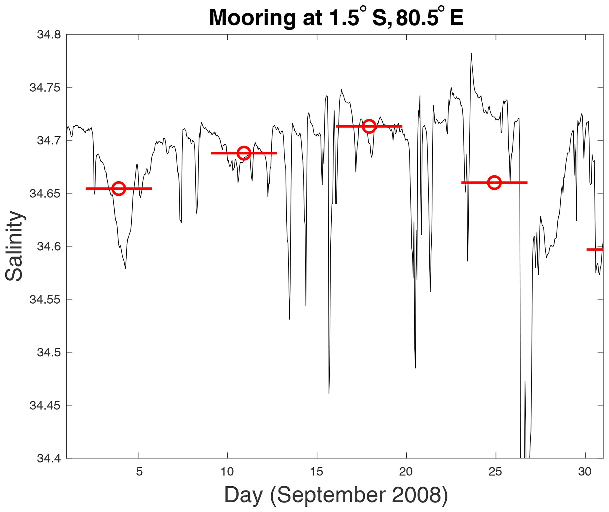
Figure 2 Sample salinity record from mooring at 1.5^∘ S, 80.5^∘ E for the month of September 2008. The weekly evaluation times are shown by red “O” symbols. The ensemble time period for this mooring was found to be ∼3.7 d. These time periods surround the evaluation times and are indicated by the red lines, which are 3.7 d long from beginning to end. The red symbols are at the mean SSS value for each ensemble time period.

To mimic the process of validating satellite measurements, we also computed a mean SSS within each ensemble time period (red symbols and lines in Fig. 2). The mean over this interval is an approximation of the footprint mean that Aquarius would have seen in one L2 sample. For illustration, we show the SSS record for one ensemble time period (∼7 d) for one mooring in Fig. 3a; the mean and the STV are also shown (respective red symbol and red lines in Fig. 3a). The STV in Fig. 3a makes up part of the distribution for the entire record at this location shown in Fig. 3b (red line). The median value of STV for this record (green line in Fig. 3b) is reported for each mooring (Fig. 4). As stated above, the validation process for satellite L2 measurements might compare them with a single in situ measurement. To get a sense of this, we choose a random value from the ensemble to simulate a float popping up into the satellite footprint or nearby in space or time (blue symbol in Fig. 3a), and compare it with the ensemble mean. This forms a time series of differences, summarized as a histogram in Fig. 3c, over the length of the record from which we can compute the RMS (green lines in Fig. 3c). This RMS is what we will call the “RE”, a single number from each mooring. The root-mean-square difference (RMSD) between the “float” value and the satellite value is what is commonly reported in validation studies (e.g., Kao et al., 2018b). In this case there is no satellite retrieval error, so the RMSD between averaged and individual values that we compute is due only to the RE. The mean difference (instantaneous value – short-term mean) for each mooring is also computed (e.g., blue line in Fig. 3c) and is reported below as the bias.

Figure 3 An example of how the STV is computed, as explained in the text. (a) A ∼7 d piece of the SSS record from the indicated mooring. The mean value is shown by the red mark, with the red bars representing ±1 standard deviation. The blue “+” is a random value picked from the record. The blue line shows the difference between the random value and the mean value. (b) The distribution of STV from the entire record at this mooring. One value is given by the standard deviation from panel (a) and is the same as the red bar in panel (b). The median of the values in this distribution is indicated by the green bar. This is the single number from this mooring that is shown as STV in Fig. 3a. (c) Distribution of differences between random samples and mean values. One value is given by the blue line in panel (a) and is the same as the blue bar in panel (c). The RMS of this distribution is shown by the green bars, which is the mean ± RMS. These bars are the single RE value that is shown for this mooring in Fig. 5b.

The GTMBA mooring time series have many gaps and missing data. The STV and RE were computed within each ensemble time period only if there were 10 or more hourly values of measured SSS.

3 Results

The median STV at each mooring (Figs. 4, 5a) mainly ranges from 0.02 to 0.15, with most between 0.02 and 0.08. In the Pacific, the values are smallest along the Equator and to the south. Larger values are found along 8^∘ N (0.06–0.11), along 95^∘ W in the eastern basin (0.08–0.11) at the edge of the eastern Pacific fresh pool (Alory et al., 2012), and in the western basin (0.04–0.10). The Atlantic Basin has some larger values, especially one of 0.3 close to the coast of Africa near the outlet of the Congo River. In the Indian Basin, large values are seen in the Bay of Bengal (0.06–0.15). This is likely due to the large input of freshwater from rivers (Akhil et al., 2020). Of all the moorings, the median value of STV is 0.05, although the distribution of values (Fig. 5a) shows a wide range.

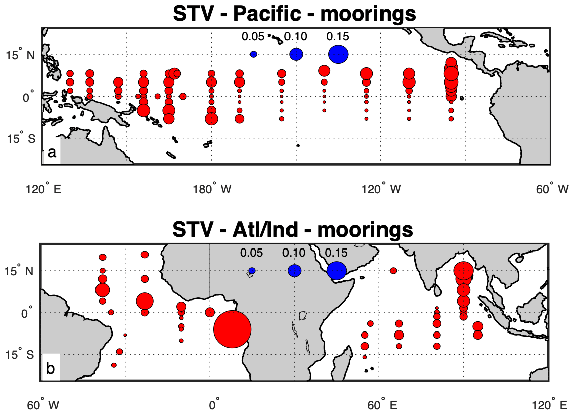
Figure 4 Median STV for each mooring for the (a) Pacific Basin and (a) Atlantic and Indian basins. The sizes of the circles indicate the magnitude of the STV, with the scale shown as blue circles near the middle of each panel.

.

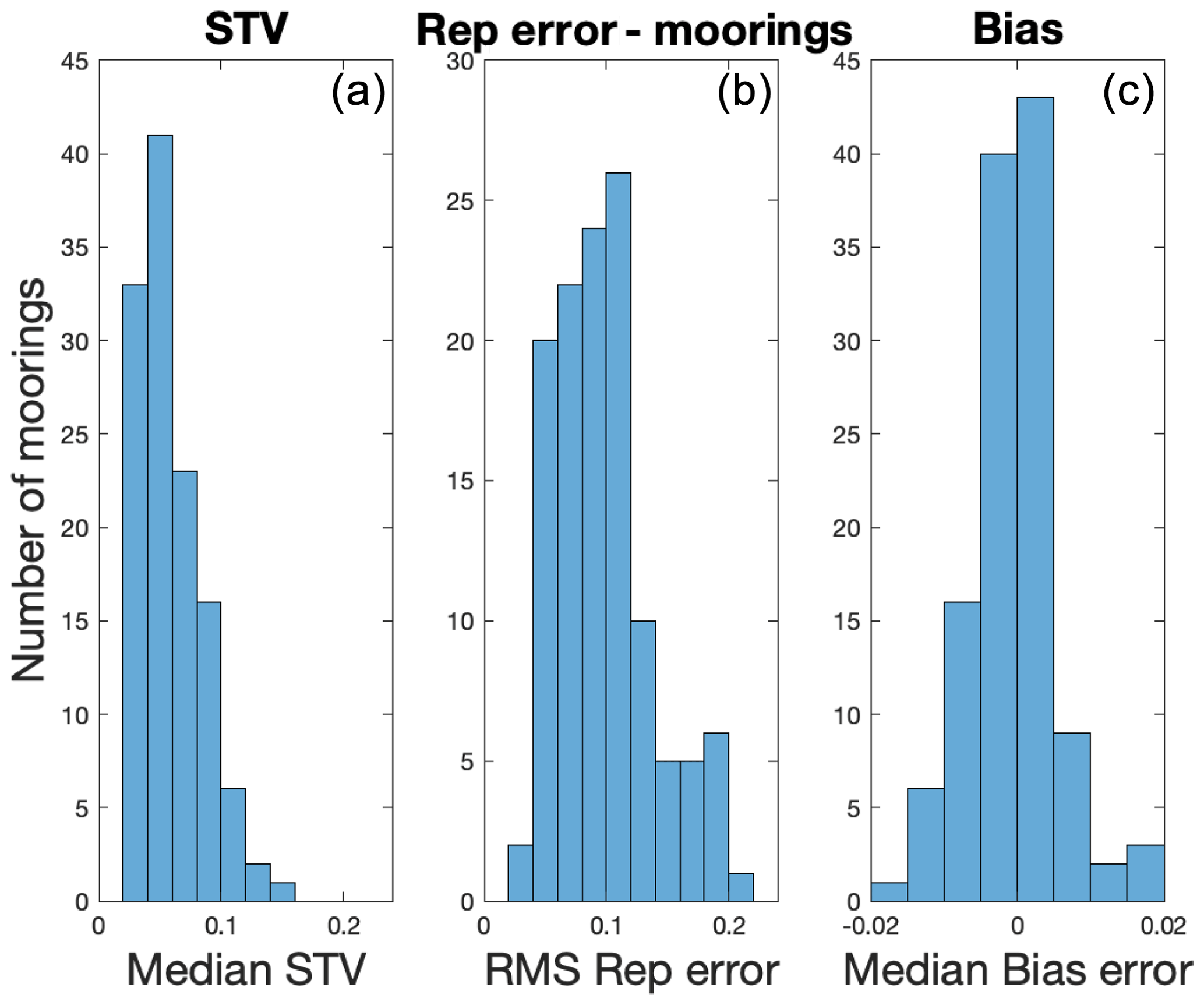
Figure 5 (a) Histogram of the median STV values shown in Fig. 4. One mooring is not included in this figure, an outlier with an STV ≈0.3 – the large symbol near the coast of Africa in Fig. 4b. Panel (b) is the same as panel (a) but for the RMS representation error shown in Fig. 6. Panel (c) is the same as panel (a) but for the bias error. Positive bias error means an instantaneous value greater than the short-term mean. Note that panels (b) and (c) rely on choosing random values from each short-term ensemble. This was done a number of times with different random values with only minor differences in results. Also note that the distributions depicted here included a small number of outliers that are not shown for clarity. Note the different x axis limits in panel (c)

The RE (Figs. 5b, 6) is generally larger than the STV. The difference is especially notable in the southwest Indian Basin. Most values of STV lie between 0.04 and 0.14 (Fig. 5b). This difference between the RE and STV may be due to the presence of outlier values in the SSS distribution (Bingham et al., 2002; Bingham, 2019). If the distribution of the SSS was close to normal, these two quantities would be about the same. This is illustrated in Fig. 3c. The green bars, which represent the RMS difference between random samples and the short-term mean, are larger than one would expect from looking at the distribution shown; this is due to the presence of a large outlier that is not pictured in the histogram. This large RMS difference value, ∼ 0.12, the green bar in Fig. 3c, is larger than the median STV for this mooring, which is about 0.03.

Although one might have expected this due to low outlier values, there is almost no bias error detected. The distribution of the median bias error is centered closely around zero, with most values less than 0.005 (Fig. 3c). There is no sign of a tendency for the bias to be positive or negative. For brevity, we do not show maps of bias error.

The STV computed from mooring data has been shown to be highly seasonal by Bingham (2019) for the two SPURS regions. To understand the degree of seasonality in the variability, we have computed the average STV in each month for the entire record at each mooring location. We display the month where STV is maximum as well as the ratio of the maximum STV to the minimum STV (Fig. 7). The amount of seasonality does depend on location. In the Pacific, it is strong in the eastern basin and along the northern portion of the GTMBA, but it is much weaker elsewhere. The seasonality is notably weak in the western Pacific, in contrast to the strong STV in this region (Fig. 4a). The Atlantic Basin displays stronger seasonality than the other two basins, especially on the eastern and western sides. The Indian Basin has relatively weak seasonality in the eastern part of the basin but stronger seasonality in the southwest. The Bay of Bengal moorings show very little seasonality, in contrast to their RE (Fig. 6b).

Figure 6 The RMS representation error at each mooring – that is, the RMS difference between random samples and short-term mean values. Panel (a) shows the Pacific Basin, and panel (b) shows the Atlantic and Indian basins. The sizes of the circles indicate the magnitude of the RE, with the scale shown as blue circles near the middle of each panel.

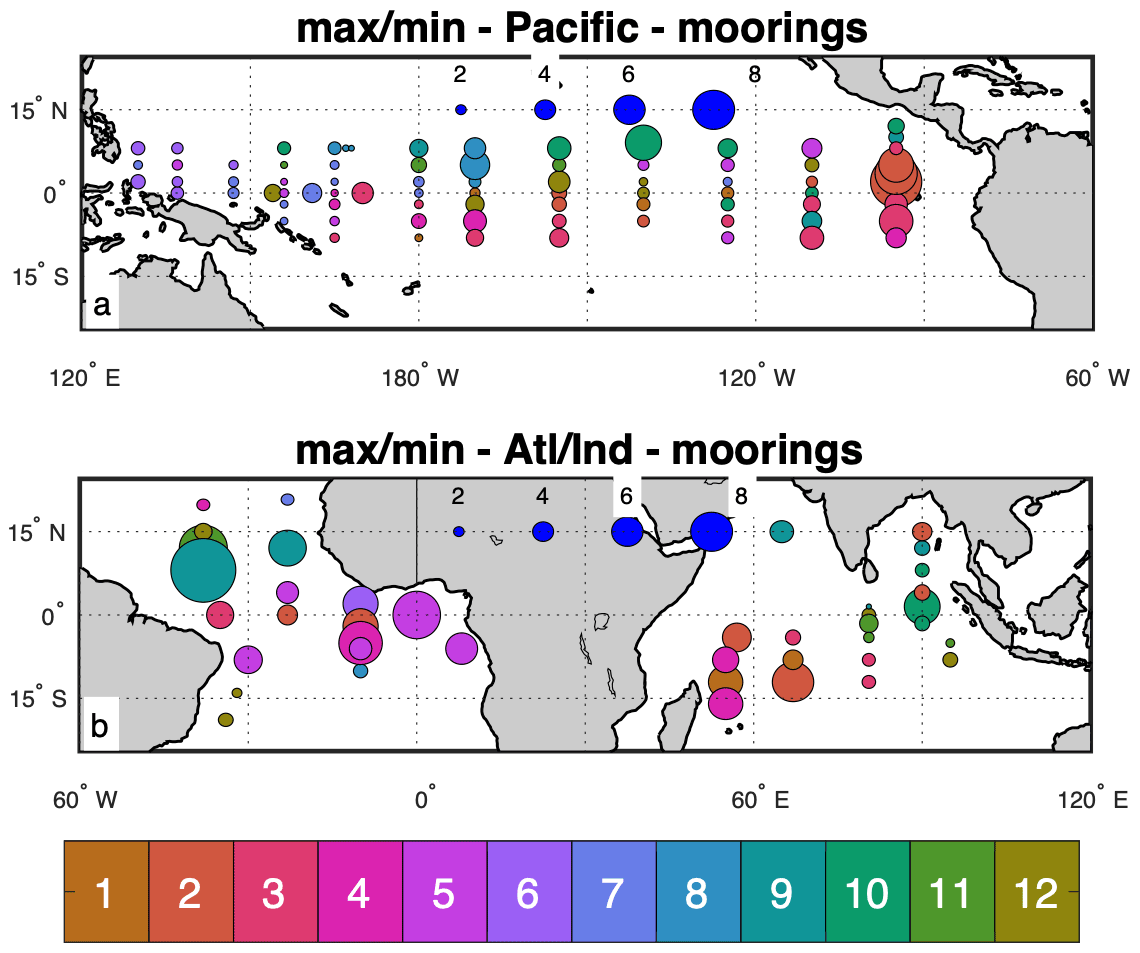
Figure 7 Ratio of the maximum value of STV to the minimum value (sizes of symbols), and the month of the maximum STV (symbol colors with scale at bottom in months, January–December). Panel (a) shows the Pacific Basin, and panel (b) shows the Atlantic and Indian basins. A size scale for the STV ratio is shown as blue circles near the middle of each panel.

The timing of maximum STV varies substantially from one part of the tropical ocean to another (Fig. 7) and is very much dependent on local conditions. STV is maximum in January–February in the eastern Pacific, as the eastern Pacific fresh pool extends to the west (Melnichenko et al., 2019). It is maximum in August–September under the Intertropical Convergence Zone (ITCZ), mixed along the Equator, and maximum in May–June in the western Pacific. In the Atlantic, STV is maximum in April–May in the eastern basin near Africa but reaches a maximum in August–September in the western basin. The western basin values are likely associated with the extension of the Amazon River plume into the central Atlantic along 5–10^∘ N (Grodsky et al., 2014). The eastern basin timing is due to the extension of the Congo River plume, which reaches its maximum extent in boreal spring (Chao et al., 2015). In the southwestern Indian Ocean, the seasonality is large, but the timing is varied from January–February to April–May. In the Bay of Bengal (BoB), the STV maximum is inconsistent, with two moorings giving maximum STV values in September–October and another giving maximum values in January. We suspect that STV variability in the BoB is closely related to river outflow (Akhil et al., 2014).

A set of maps of STV from the MITgcm output (Fig. 8) has many similarities to those derived from the moorings (Fig. 4); however, the values are generally smaller. Larger values are found in the eastern and western tropical Pacific, the Atlantic north of the Equator, and the Bay of Bengal. Notably, the row of locations along 8^∘ N in the North Pacific does not exhibit the large variability seen in the mooring data (Fig. 4a). The STV in the outflow of the Congo River near the coast of Africa is much smaller in the model than in the mooring data, possibly due to the model's use of climatological river outflow (Feng et al., 2021; Fekete et al., 2002). A similar set of maps for the RE was created for the model output but is not included here for brevity. We do include histograms of STV, RE, and bias (Fig. 9) for comparison with the mooring data (Fig. 5). The distributions from the model are again similar to those from the moorings, although somewhat smaller. Table 1 gives median values of the distributions of STV and RE, showing larger values for the observed data. A direct comparison of STV from the moorings vs. the model indicates that the mooring STV is larger in most cases (Fig. 10), but the two have a close relationship. In only about 10 % of the mooring locations is the model STV greater than the mooring STV.

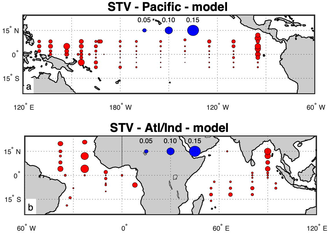
Figure 8 The same as Fig. 4 but for STV computed from the MITgcm. Panel (a) shows the Pacific Basin, and panel (b) shows the Atlantic and Indian basins.

Table 1 Median values for all of the moorings and mooring locations from the distributions of Figs. 5 and 9.

Figure 9 The same as Fig. 5 but for values computed from the MITgcm.

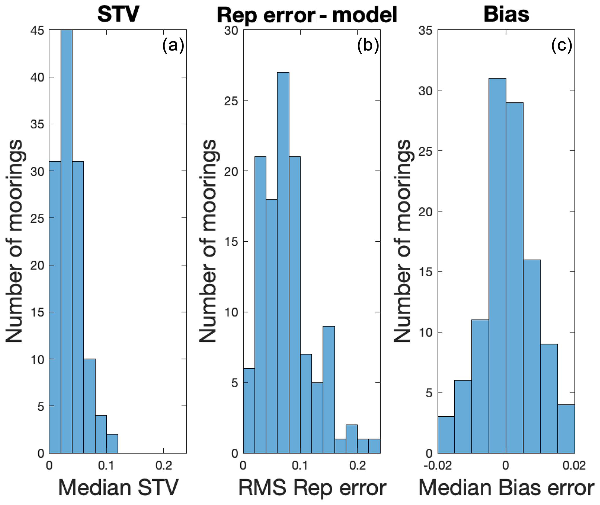
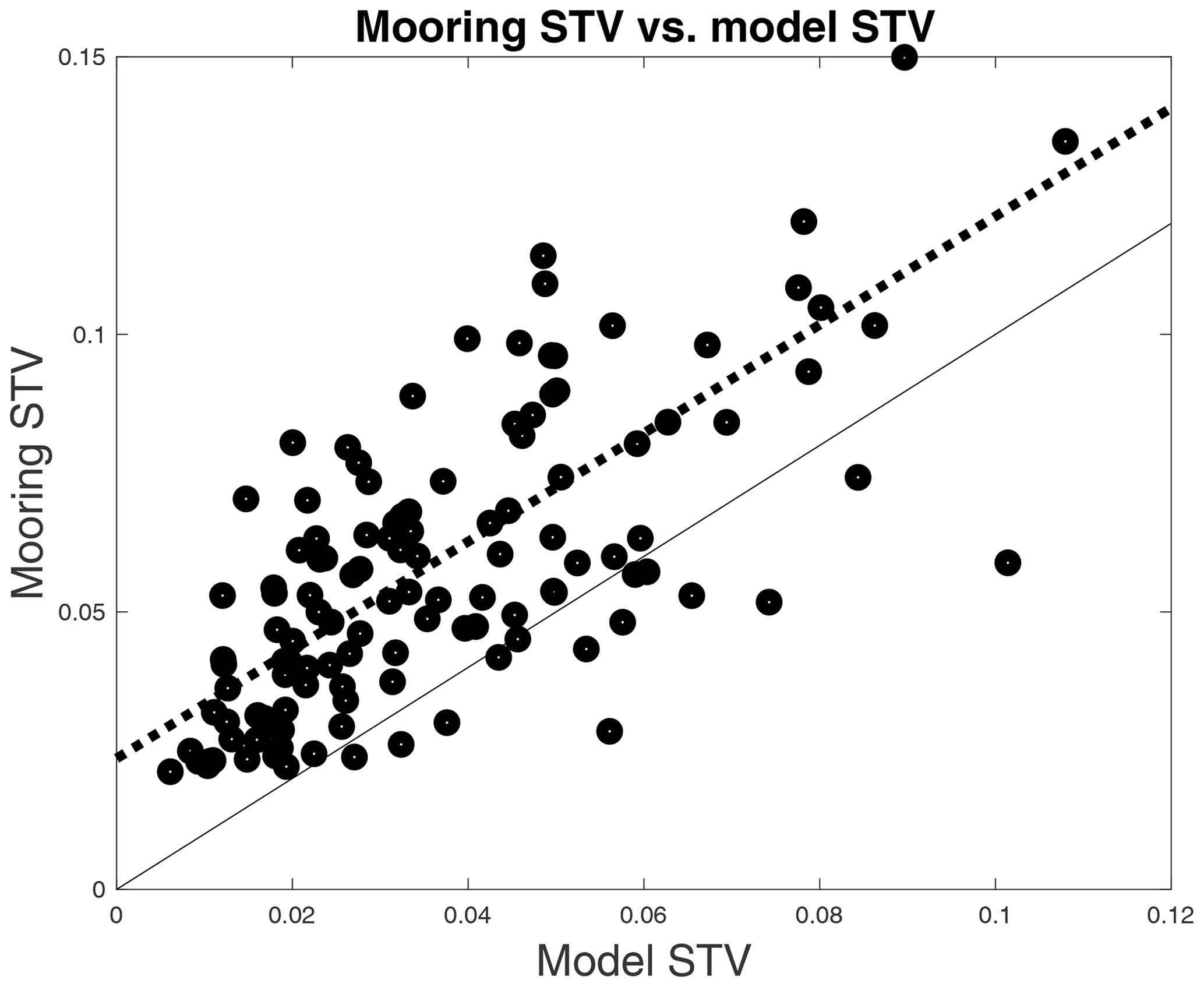
Figure 10 Model STV vs. mooring STV. Each symbol represents the median STV for one mooring. A couple of outlier points have been omitted for clarity. The dashed line is a least-squares fit to the data. It has a slope of about 1 and an intercept of about 0.02. The light black line has a slope of 1. This plot indicates that the mooring STV is generally larger than the model STV.

STV may be mainly caused by rainfall, by internal variability in the mesoscale or submesoscale SSS field of the ocean, or by the motion of large-scale fronts (Drushka et al., 2019). It is difficult to measure these effects separately to disentangle them. One problem with measuring the impact of rainfall on STV is that it has a strange distribution, with hourly values being mostly zero even during rainy periods (e.g., Bingham et al., 2002, their Fig. 11). Many of the GTMBA moorings, 88 out of 123, have precipitation measurements. To measure the impact of rainfall on STV, we used those records to determine the maximum rain rate over each ensemble period. We then found the STV during periods when the maximum rain rate was greater than 1 mm hr⁻¹ and during periods when it was less than 1 mm hr⁻¹. For almost every mooring (78 out of 88) the STV during rainy periods was greater than during non-rainy periods. A typical example of this is presented in Fig. 11. Because of the way rainfall is distributed, it does not make sense to compute correlations between maximum rain rate and STV, which can be easily seen in Fig. 11. Thus, we report the apparent connection here in this simple way, concluding that STV is indeed at least partly driven by rainfall.

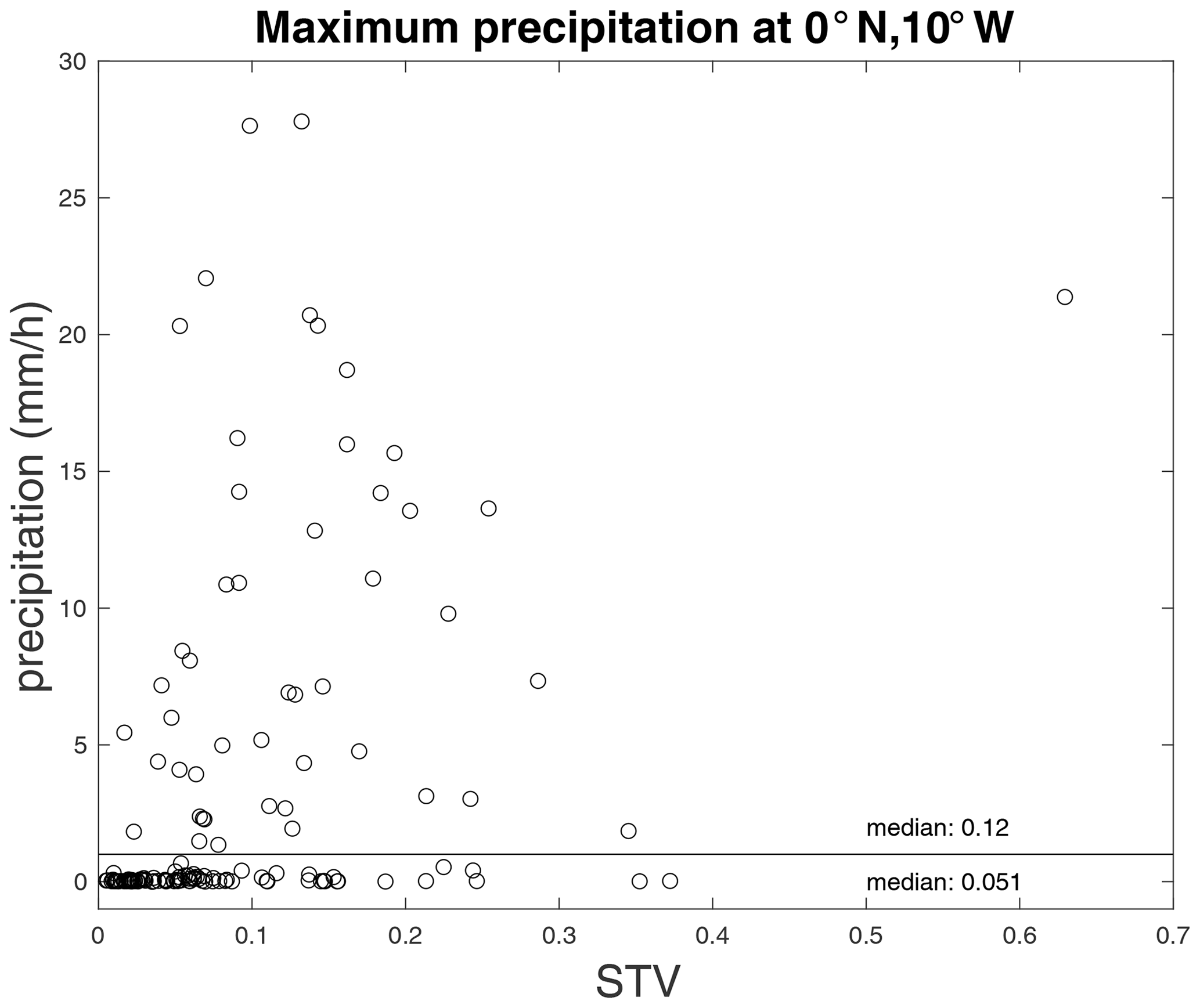
Figure 11 An example of how STV relates to precipitation at one mooring location. Maximum hourly precipitation for each short-term ensemble for the mooring (at 0^∘ N, 10^∘ W) vs. STV for the same set of ensembles. The light line indicates a rain rate of 1 mm hr⁻¹, separating rainy periods from non-rainy ones. Median values for all ensembles with a maximum precipitation of less than 1 mm hr⁻¹ (below the line) and greater than or equal to 1 mm hr⁻¹ (above the line) are shown in the bottom right. These values indicate that STV tends to be greater when there is rainfall. However, there is not a clear correlation between rainfall and STV. This pattern was consistent in most of the GTMBA moorings with precipitation records.

A non-result that is important to report here is the lack of temporal aliasing. One might expect, within the ensemble time periods that we used, that the difference between the short-term mean (e.g., red symbol in Fig. 3a) and the random samples that we took (e.g., blue symbol in Fig. 3a) would increase with the difference in time between the samples and the mean times. We plotted this for each mooring and uniformly found there to be no relationship between the two. The ensemble time periods that we used were too short for there to be changes in the statistics of the SSS field.

4 Discussion

We have computed values for STV and RE that can be factored into error budgets of satellite SSS. The values in Table 1 are typical, but there is a large range (Figs. 4–6). If anything is clear from the analysis done here, it is that STV and RE depend on both time and space. In many areas studied here, especially the equatorial Pacific, STV is small and would be negligible compared with other sources of error in L2 satellite estimates. In other areas, such as the Bay of Bengal, the western North Atlantic, and the eastern and western Pacific, STV is important and could play a larger or even dominant role in the error budget.

As stated in Sect. 2, the STV is used here as a proxy for SFV over a 100 km footprint – that is, it is the variability over a 100 km spatial scale surrounding each mooring. This use depends on the assumption that the velocity field that we used, which is derived from OSCAR, is generally representative of that experienced by the mooring. This is needed to make the jump from our estimate of STV to that of SFV. More subtly, the region sampled is that parallel to the flow at the mooring. The scheme that we have used does not sample across the flow field. Thus, we have assumed that the spatial variability across the direction of flow is similar to that along the direction of flow. Without simultaneous sampling in a spatial region surrounding the moorings (e.g., Bingham, 2019; Reverdin et al., 2015), it is impossible to know how much variation is being missed. We were able to compute SFV at each mooring location from the MITgcm for comparison to STV from the model (Fig. 12). This result shows that STV and SFV have a close relationship and that it makes sense to use one as a proxy for the other. Figure 12 suggests that STV is about half of the true SFV. Thus, the values given in Table 1 as estimates of STV might be multiplied by 2 to get estimates of SFV at the mooring locations.

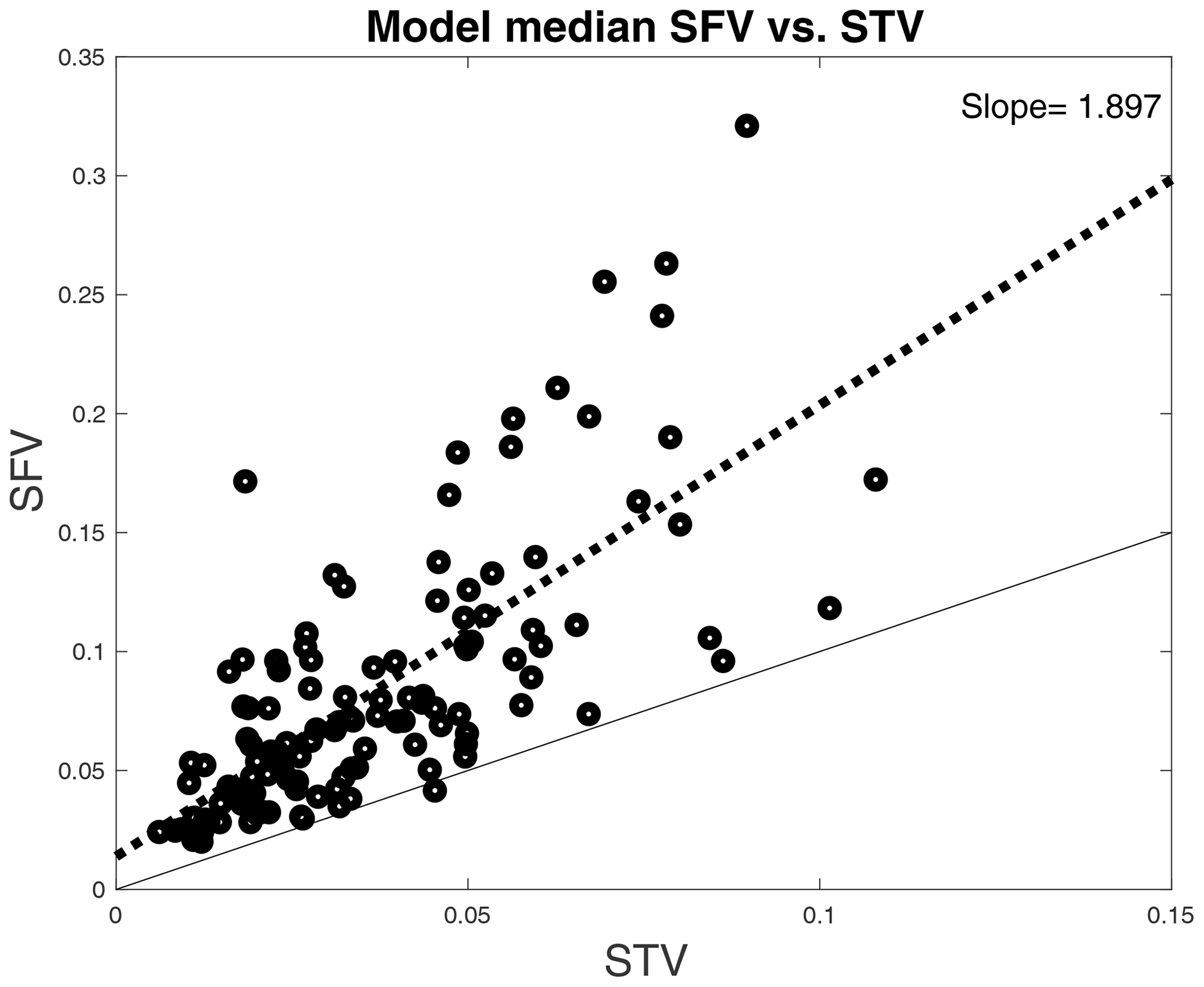
Figure 12 Median model SFV vs. model STV at each mooring location. Each symbol represents one mooring. The light line has a slope of 1. The dashed black line is a least-squares fit to the data shown, with the slope indicated in the top right.

The main purpose of this work is to understand subfootprint variability and representation error and its impact on the satellite measurement of SSS. This type of analysis is a good test for the MITgcm and could be used for other models. The fact that STV is lower in the model than for the moorings suggests that either the model resolution is not quite good enough to match the statistics of the real ocean or (more likely) that the forcing fields used, especially the rainfall, are too coarse compared with the real forcing. It is clear that rainfall occurs on a scale that is smaller than what the typical ocean model is exposed to (Bingham and Li, 2020; Thompson et al., 2019). The atmosphere continually adds small-scale variance to the ocean in the form of freshwater forcing. It would be interesting to see how the scale of the input freshwater forcing variance affects the behavior of forced models like the one that we used.

The numbers in Table 1 can be thought of as an estimate of “snapshot error” (Bingham, 2019) due to representation. This is the error in each L2 estimate captured by a SSS satellite as it passes overhead due to variability within the satellite footprint. Most estimates of SSS error are computed at L3 (e.g., Qin et al., 2020; Olmedo et al., 2021). The production of L3 values entails combining numerous individual L2 snapshots into a gridded product on a quasi-weekly or monthly basis using some form of optimal interpolation (Melnichenko et al., 2014, 2016) or bin-averaging (Vergely and Boutin, 2017). Thus, the numbers in Table 1 and Fig. 4 are a worst case, consisting of errors that can be averaged out in the process of moving from L2 to L3 – assuming they are random. In a sense, this is a hopeful sign. The numbers in Table 1 are much smaller than the total errors associated with satellite retrieval including surface roughness, galactic reflection, etc. (Olmedo et al., 2021; Meissner et al., 2018). However, a more granular analysis, like that in Fig. 6, suggests that it may not be that simple. There are times and places where REs may be significant, such as the eastern Pacific, the Bay of Bengal, and river plume regions. These are all regions where higher-SSS open-ocean waters interact intermittently with much lower-SSS coastal or river plume water. Thus, it may make sense, when computing RMS errors for satellite retrievals, to leave these areas out of the analysis or to somehow account for the larger amounts of RE that may be present in the L2 measurements there.

There is a remarkable similarity between the STV in Fig. 3 and the amplitude of the annual cycle shown by Bingham et al. (2021, their Fig. 3). The relative sizes of the symbols are very similar in most cases. There are a few exceptions. Areas with relatively large STV but small seasonal amplitude include the region of the South Pacific under the South Pacific Convergence Zone, some areas of the central and western south Indian Ocean, the Bay of Bengal, and a couple of the moorings in the western tropical North Atlantic. Most of these areas have small amplitude in seasonal precipitation compared with the rest of the tropics (see Bingham et al., 2012, their Fig. 11e). Thus, regions with large (small) seasonal variability are also ones with large (small) STV. As STV appears to be somewhat driven by rainfall (Fig. 11), this makes sense. Many tropical regions, like the Northern Hemisphere ITCZ, with heavy rainfall are also areas that experience strong seasonality in rainfall.

The vague nature of the relationship between rainfall and STV is highlighted in Fig. 11 and similar single-mooring analyses that we do not show. The original concept for satellite SSS is that it could be used as a rain gauge (Lagerloef et al., 2008). This may be more complicated than originally thought, at least for the short-term relationship. Work into the use of SSS as a rain gauge (Supply et al., 2018), i.e., a way to estimate precipitation over the ocean, is ongoing. Doing this with mooring precipitation and SSS data will require a much more sophisticated approach than we have attempted here. At the very least, perhaps SSS can be used to detect whether rain is happening or not.