Flow separation, dipole formation, and water exchange through tidal straits

We investigate the formation and evolution of dipole vortices and their contribution to water exchange through idealized tidal straits. Self-propagating dipoles are important for transporting and exchanging water properties through straits and inlets in coastal regions. In order to obtain a robust dataset to evaluate flow separation, dipole formation and evolution, and the effect on water exchange, we conduct 164 numerical simulations, varying the width and length of the straits as well as the tidal forcing. We show that dipoles form and start propagating at the time of flow separation, and their vorticity originates in the velocity front formed by the separation. We find that the dipole propagation velocity is proportional to the tidal velocity amplitude and twice as large as the dipole velocity derived for a dipole consisting of two point vortices. We analyze the processes creating a net water exchange through the straits and derive a kinematic model dependent on dimensionless parameters representing strait length, dipole travel distance, and dipole size. The net tracer transport resulting from the kinematic model agrees closely with the numerical simulations and provides an understanding of the processes controlling net water exchange.

1 Introduction

Knowledge of coastal ocean transport processes is vital for predicting human impact on the coastal marine environment. Coastal industry discharges pollutants and nutrients into the ocean. In order to understand the impact on the environment, we need coastal ocean circulation models to calculate concentrations and pathways of spreading. Setting up such models for a complex coastline requires a high level of understanding of nearshore transport processes in order to realistically represent these in the models. In shallow coastal regions with complex topography, tides are often a dominant driver of the ocean circulation and transport. In this study, we investigate the exchange process of tidal pumping through narrow tidal straits.

Tidal pumping is an important mechanism responsible for transport of water properties and particles like fish eggs, nutrients, and pollution between estuaries and the open ocean or in coastal regions with complex geometry in general (Chadwick and Largier, 1999; Fujiwara et al., 1994; Brown et al., 2000; Amoroso and Gagliardini, 2010; Ford et al., 2010; Vouriot et al., 2019). The exchange process results from an asymmetry in the flow field between the ebb and flood phase of the tide (Stommel and Farmer, 1952; Wells and van Heijst, 2003). Flow asymmetry may occur when the tidal current interacts with a topographic constriction like a strait or an inlet. When entering the constriction the flow arrives from all directions and speeds up in order to conserve volume, as illustrated by Fig. 1a. The area covered by the volume that enters the strait is called the sink region (Fig. 1a). The acceleration is associated with a pressure force towards the constriction, which acts to lower the water level in the center of the constriction. In contrast, when the flow reverses and the flow exits the strait, the cross-sectional area increases and the sea surface rises downstream of the constriction. Here, both friction and pressure forces work to decelerate the flow, which is a necessary condition for flow separation (Kundu, 1990). Since friction and pressure now work in the same direction, the flow is likely to come to a halt near the coastline where the friction is strongest. When this happens, the flow separates from the coastline as illustrated by Fig. 1b (Kundu, 1990; Signell and Geyer, 1991). When the flow separates a vortex forms at the point of separation. If the flow separates at both sides of the exit, two vortices of opposite sign will form with a separation distance roughly equal to the width of the strait. The strength of the vortices and the distance between them determine whether they will interact and form a self-propagating dipole. The dipoles capture and transport water ejected from the strait away from the opening and possibly out of the sink region. At flow reversal, the dipole will either be drawn back into the strait or continue moving away and escape. If the dipole escapes the return flow it will contribute to considerable water exchange (Fig. 1b).

Figure 1 A sketch of the processes at play in water exchange by tidal pumping. (a) Southward inflow to the strait. (b) Northward outflow from the strait.

The propagation of dipoles has been studied for more than 100 years (Lamb, 1916; Batchelor and Batchelor, 2020; Kundu, 1990), and the velocity of a self-propagating dipole is typically represented as

$$\begin{array}{}\text{(1)}& U_{\mathrm{dip}}={\displaystyle \frac{\mathrm{\Gamma }}{\mathrm{2}\mathit{\pi }b}}.\end{array}$$

Here b is the distance between the vortex centers, and Γ is the magnitude of the circulation in each of the two vortices, assuming they are of equal strength. Equation (1) is valid as long as the distance between the two vortices is large compared to their core radius (Yehoshua and Seifert, 2013; Delbende and Rossi, 2009; Habibah et al., 2018). Habibah et al. (2018) show that a correction to the velocity given by Eq. (1) occurs in the fifth order of $a/b$, where a is the core radius of the vortices. In cases in which $a/b$ increases, the vortices becomes elliptical and the dipole propagation velocity decreases (Delbende and Rossi, 2009).

Equation (1) describes the propagation velocity of a dipole moving by self-propagation in an otherwise nonmoving ocean. It is unclear whether this is valid for a dipole formed in a tidal strait, where the background flow is clearly nonzero. Also, dipoles propagating away from the strait often remain attached to the strait via a trailing jet (Fig. 1b), which provides a pathway of mass, momentum, and vorticity from the strait into the dipole (Wells and van Heijst, 2003; Afanasyev, 2006). As the dipole accumulates vorticity the circulation in the dipole increases, and the propagation velocity should therefore accelerate according to Eq. (1). However, this is not necessarily true. In a lab experiment investigating dipole formation by a steady channel jet, Afanasyev (2006) found that the dipole propagated with constant speed, even though the dipole continuously accumulated vorticity fed by a trailing jet.

The circulation of the dipole vortices is an important parameter for determining the propagation velocity, and to determine the circulation it is vital to know the source of vorticity. A common assumption is that the vorticity is created in the viscous boundary layer (Wells and van Heijst, 2003; Nicolau del Roure et al., 2009; Bryant et al., 2012). Another possible source is the flow discontinuity resulting when the flow separates from the coastline (Kashiwai, 1984a, b). Kashiwai (1984a, b) and Wells and van Heijst (2003) both assume that all vorticity generated in the strait accumulates in the dipole vortices. The circulation can then be expressed as Γ∝U²T, where T is the tidal period and U is a characteristic velocity scale for the strait (Kashiwai, 1984b; Wells and van Heijst, 2003). However, Afanasyev (2006) showed that the vorticity is divided between the dipole and the trailing jet. In addition, Afanasyev (2006) introduced a new timescale, which he called the “startup time”, t_s. The startup time indicates the moment when the dipole starts translating after an initial period of growth, during which the jet is injected into the dipole.

The net tracer transport through a tidal strait is commonly classified by the nondimensional Strouhal number, S_t, defined as (Kashiwai, 1984a; Wells and van Heijst, 2003; Nicolau del Roure et al., 2009)

$$\begin{array}{}\text{(2)}& S_{\mathrm{t}}={\displaystyle \frac{W}{UT}},\end{array}$$

where W is the strait width, T is the tidal period, and U is the velocity scale characterizing the velocity in the strait. W can also be seen as a characteristic spatial scale of a dipole formed at the strait exit, and in this case S_t is a measure of the ratio between linear and nonlinear acceleration terms. The centers of the dipole vortices are pressure minima, and the nonlinear acceleration associated with the azimuthal velocity of the vortices is balanced by pressure forces. Thus, for a dipole vortex to exist, S_t≪1 is a necessary condition.

Net tracer transport by tidal pumping is associated with S_t<S_tc, where S_tc is a threshold value of S_t (Kashiwai, 1984a; Wells and van Heijst, 2003). The threshold value of the Strouhal number arrives from a kinematic consideration of the dipole movement over one tidal period and separates between dipoles that escape the return flow and the dipoles that return to the strait during the subsequent phase of the tide (Kashiwai, 1984a; Wells and van Heijst, 2003). Dipoles escaping the return flow contribute to net water exchange through the strait. A threshold value of S_tc=0.13 was found by Wells and van Heijst (2003), and this value was later confirmed by Vouriot et al. (2019) in a numerical study of idealized tidal lagoons.

In this study, our aim is to understand how the geometric constraint of a tidal strait influences the effectivity of tidal pumping. We systematically perform 164 numerical simulations in an idealized tidal strait, varying the width and length of the straits as well as the amplitude of the tidal forcing. Although 3D processes may affect vortex flows (van Heijst, 2014; Albagnac et al., 2014), we believe a 2D depth-averaged approach will give valuable new insight into tidal strait flows. A 2D approach is therefore used in this study. The results of the simulations are analyzed with a focus on flow separation, dipole formation and propagation, and net water exchange. Finally, we derive a simple kinematic model for net tracer transport that fits the results from the simulations well and brings understanding to the process of water exchange through a tidal strait.

2 Modeling

2.1 The model

We use the Finite Volume Community Ocean Model (FVCOM) (Chen et al., 2003). FVCOM has been used in numerous studies of coastal and estuarine waters (Lai et al., 2015, 2016; Sun et al., 2016; Li et al., 2018; Chen et al., 2021) and also globally and in the Arctic Ocean (Chen et al., 2016; Zhang et al., 2016). FVCOM uses an unstructured triangular grid in the horizontal and terrain-following σ coordinates in the vertical (Chen et al., 2003). The model solves the equations for momentum and mass conservation as well as the equations for temperature, salinity, and density. In our case, we set temperature, salinity, and density to constant values and FVCOM then solves the following equations.

$$\begin{array}{}\text{(3)}& \begin{array}{rl}{\displaystyle \frac{\partial u}{\partial t}}& +u{\displaystyle \frac{\partial u}{\partial x}}+v{\displaystyle \frac{\partial u}{\partial y}}+w{\displaystyle \frac{\partial u}{\partial z}}-fv\\ & =-{\displaystyle \frac{\mathrm{1}}{{\mathit{\rho }}_{\mathrm{0}}}}{\displaystyle \frac{\partial p}{\partial x}}+{\displaystyle \frac{\partial }{\partial z}}\left(K_m{\displaystyle \frac{\partial u}{\partial z}}\right)+F_u\\ & {\displaystyle \frac{\partial v}{\partial t}}+u{\displaystyle \frac{\partial v}{\partial x}}+v{\displaystyle \frac{\partial v}{\partial y}}+w{\displaystyle \frac{\partial v}{\partial z}}+fu\\ & =-{\displaystyle \frac{\mathrm{1}}{{\mathit{\rho }}_{\mathrm{0}}}}{\displaystyle \frac{\partial p}{\partial y}}+{\displaystyle \frac{\partial }{\partial z}}\left(K_m{\displaystyle \frac{\partial v}{\partial z}}\right)+F_v\\ & {\displaystyle \frac{\partial u}{\partial x}}+{\displaystyle \frac{\partial v}{\partial y}}+{\displaystyle \frac{\partial w}{\partial z}}=\mathrm{0}\\ & {\displaystyle \frac{\partial p}{\partial z}}=-{\mathit{\rho }}_{\mathrm{0}}g\end{array}\end{array}$$

Here, x, y, and z are the Cartesian coordinates in the east, north, and vertical directions, respectively; u, v, and w are the x, y, and z components of velocity, respectively; p is pressure; ρ₀ is the constant density; f is the Coriolis parameter; g is the acceleration of gravity; K_m is the eddy diffusion coefficient; and F_u and F_v are the diffusion terms for horizontal momentum in the x and y directions, respectively. The calculation of K_m is done with the Mellor and Yamada (1982) level 2.5 turbulent closure scheme, modified by Galperin et al. (1988). F_u and F_v are calculated using the eddy parameterization method by Smagorinsky (1963). The diffusion coefficient within F_u and F_v is given by

$$\begin{array}{}\text{(4)}& A_m=\mathrm{0.5}C\mathrm{\Omega }\sqrt{{\left({\displaystyle \frac{\partial u}{\partial x}}\right)}^{\mathrm{2}}+\mathrm{0.5}{\left({\displaystyle \frac{\partial v}{\partial x}}+{\displaystyle \frac{\partial u}{\partial y}}\right)}^{\mathrm{2}}+{\left({\displaystyle \frac{\partial v}{\partial y}}\right)}^{\mathrm{2}}},\end{array}$$

where C is a constant, set to 0.1 in our case, and Ω is the grid cell area.

The surface boundary conditions are

$$\begin{array}{}\text{(5)}& \left.\begin{array}{l}{K}_m\left(\frac{\partial u}{\partial z},\frac{\partial v}{\partial z}\right)=\frac{\mathrm{1}}{{\mathit{\rho }}_{\mathrm{0}}}\left({\mathit{\tau }}_{\mathrm{s}x},{\mathit{\tau }}_{\mathrm{s}y}\right)\\ w=\frac{\partial \mathit{\zeta }}{\partial t}+u\frac{\partial \mathit{\zeta }}{\partial x}+v\frac{\partial \mathit{\zeta }}{\partial y}\end{array}\right|z=\mathit{\zeta }(x,y,t),\end{array}$$

where τ_sx and τ_sy are the surface stress in the x and y directions, respectively, and ζ is the surface elevation. The bottom boundary conditions are

$$\begin{array}{}\text{(6)}& \left.\begin{array}{l}{K}_m\left(\frac{\partial u}{\partial z},\frac{\partial v}{\partial z}\right)=\frac{\mathrm{1}}{{\mathit{\rho }}_{\mathrm{0}}}\left({\mathit{\tau }}_{\mathrm{b}x},{\mathit{\tau }}_{\mathrm{b}y}\right)\\ w=-u\frac{\partial H}{\partial x}-v\frac{\partial H}{\partial y}\end{array}\right|z=-H(x,y),\end{array}$$

where τ_bx and τ_by are the bottom stresses in the x and y direction, respectively, and H is the bottom depth. The bottom stresses are given by

$$\begin{array}{}\text{(7)}& \left({\mathit{\tau }}_{\mathrm{b}x},{\mathit{\tau }}_{\mathrm{b}y}\right)={\mathit{\rho }}_{\mathrm{0}}{C}_{\mathrm{d}}\sqrt{u^{\mathrm{2}}+v^{\mathrm{2}}}(u,v),\end{array}$$

where the drag coefficient is

$$\begin{array}{}\text{(8)}& C_{\mathrm{d}}=\max \left({\displaystyle \frac{{\mathit{\kappa }}^{\mathrm{2}}}{\ln {\left(\frac{z_{\mathrm{b}}}{z_{\mathrm{0}}}\right)}^{\mathrm{2}}}},\mathrm{0.0025}\right).\end{array}$$

Here, κ is the von Karman constant (∼0.4), z₀ is the bottom roughness set to be 0.001 m, and z_b is height above the bottom of the lowest horizontal velocity level.

Figure 2 Left panel: the entire model domain with the peninsula attached to the eastern coast and the island located west of the peninsula. Red marks the area with initial tracer concentration equal to 1 m⁻³. Right panel: the mesh near the strait with 12 km width (top) and 1 km width (bottom).

2.2 Setup of simulations

The model domain is bounded by a semi-circled open ocean and a straight coastline on the eastern side (Fig. 2). The full domain is 500 km in the north–south direction and up to 250 km in the east–west direction. At the center of the eastern boundary, we place a peninsula and an island separated by a strait. The strait is the focus of our study. The idea behind this configuration is that the pressure difference over the length of the strait is set by the tidal wave traveling in the open ocean and not by the flow through the strait. In this way, the flow through different strait geometries will be forced similarly. The setup can be seen as an idealized representation of the Lofoten peninsula in northern Norway.

Surface stress (Eq. 5) is set to zero, and the only forcing of the simulations is a northward-propagating Kelvin wave specified at the semi-circled western boundary:

$$\begin{array}{}\text{(9)}& {\mathit{\zeta }}_{\mathrm{obc}}=A_{\mathrm{t}}{e}^{\frac{\left(x-x_{\mathrm{c}}\right)}{R_{\mathrm{d}}}}\sin (ky-\mathit{\omega }t).\end{array}$$

Here, $\mathit{\omega }=\mathrm{2}\mathit{\pi }/T$, T is the M2 tidal period (12.42 h), $k=\mathit{\omega }/\sqrt{gH}$, x_c is the constant position along the x axis of the straight eastern coast (ignoring the peninsula), and R_d is the Rossby radius of deformation. Equation (9) describes a classical Kelvin wave moving northward with the coast to the right (Gill, 1982). The Coriolis parameter corresponds to 70^∘ N latitude and the depth H=100 m, giving a Rossby radius of R_d≃230 km. The surface elevation given by Eq. (9) is specified at the boundary nodes. The velocities in FVCOM are located in the center of each triangular cell and not directly at the boundary. The velocities in the open boundary cells are calculated based on the assumption of mass conservation (Chen et al., 2003; Chen et al., 2011).

In order to investigate the geometric effects on the tidal pumping, we vary the width of the strait, W, from 1 to 12 km and the length of the strait, L, from 4 to 22 km. The curvature of the coastline at the strait entrance and exit is equal and shaped as a quarter of a circle with a radius of R=2 km. The strait is directed north–south, and the geometry and coordinates used in the study are shown in Fig. 3b. In total we conduct 164 idealized simulations using 82 different strait geometries and two different amplitudes of the tidal forcing (A_t=1 and A_t=0.5; see Eq. 9).

We simulate a homogeneous ocean over a flat bottom of 100 m depth. To avoid unwanted effects of boundary layers near a vertical wall, we use a sloping bottom at the innermost 600 m from the coastline inside the strait (Fig. 3a). The minimum depth is 5 m. Because our tracer model requires vertical layering, we divide the water column into two layers in the vertical. However, the analysis of results is done using vertically averaged velocities, and this work can therefore be regarded as a 2D barotropic study. z_b is roughly equal to a quarter of the total depth, resulting in a slightly increased drag coefficient over the shallow depths near the sides of the strait (Eq. 8). z_b=1 m gives C_d=0.0034, while C_d=0.0025 for z_b>2.8 m.

Inside the strait the resolution is 50 m along the coastline. Inside the focus region surrounding the strait the resolution linearly coarsens to 200 m with distance from the coast. The focus region is, in addition to the strait itself, the semi-circle (radius = $W/\mathrm{2}+\mathrm{2}R$) of high resolution at both sides of the strait entrances (Fig. 2). Outside the focus area, the resolution coarsens further to 2 km both at the western tip of the island and at the coastline to the east. At the western open boundary the resolution is 20 km.

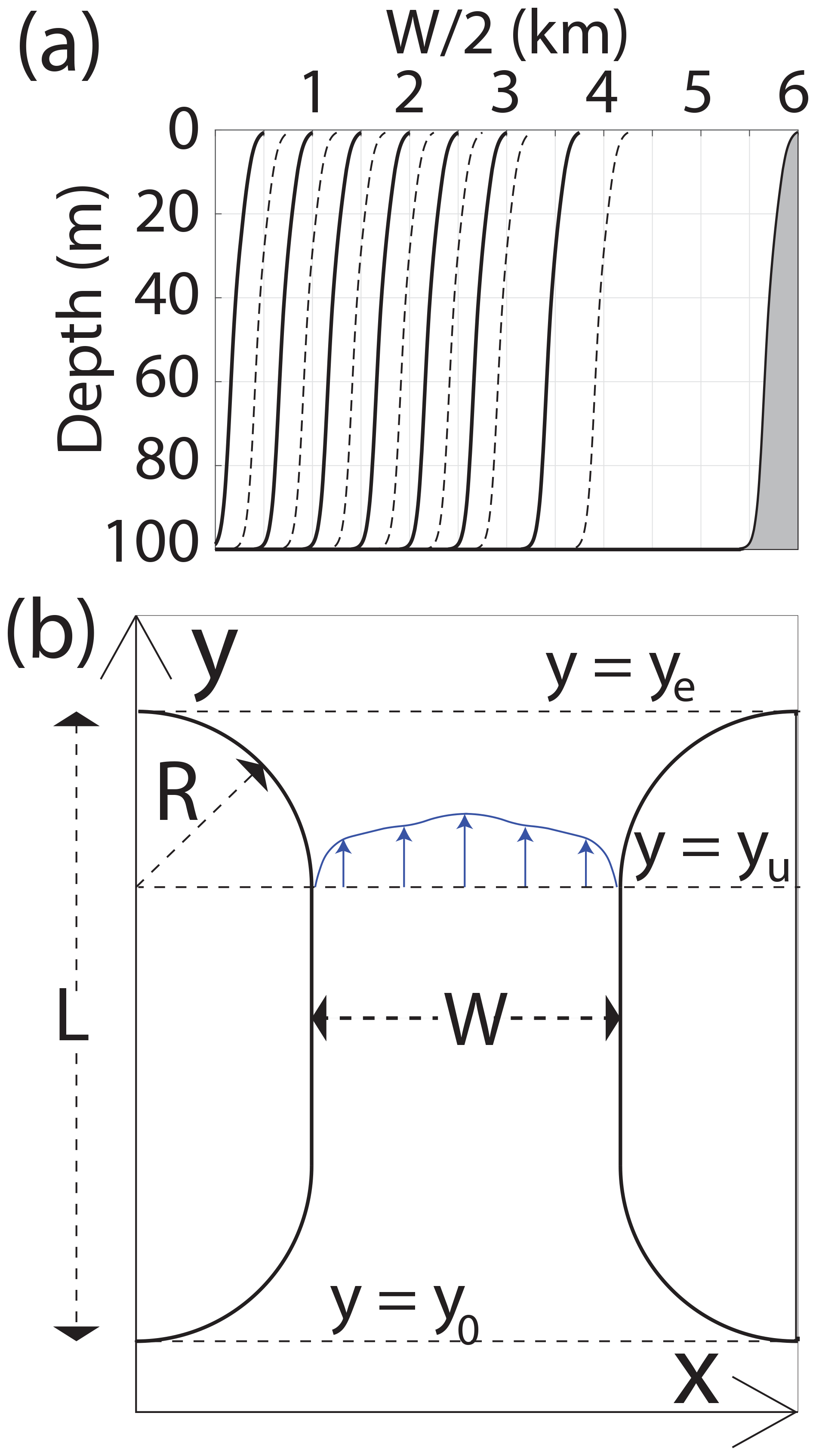
Figure 3 (a) Vertical cross section of bottom topography from the strait center to the eastern coastline for the different strait widths. The solid and dashed lines are used to more easily differentiate between the different strait widths. (b) The coordinate system of the strait configuration.

The simulations are run for a total of 20 d. First, a 10 d spin-up is done before we introduce a passive tracer, which is simulated using the Framework for Aquatic Biogeochemical Models (Bruggeman and Bolding, 2014, FABM) coupled to FVCOM. The initial concentration of the tracer is set to 1 m⁻³ inside a rectangular box south of the strait and 0 m⁻³ elsewhere (left panel in Fig. 2). The northern edge of the initial tracer release is at the center of the strait. This configuration of the initial concentration restricts the tracer exchange in the north–south direction to be through the strait only.

3 Overview of model results

By visual inspection we see that vortices form in all the different strait configurations. However, only a fraction of the straits produces self-propagating dipoles. Figure 4 provides an overview of all the simulations and the straits where self-propagating dipoles are visually observed. The dipole formation clearly depends on the strait geometry, with narrow and short straits favoring dipole formation. Additionally, with stronger tidal forcing (A_t=1.0 m) dipoles form in wider and longer straits compared to when the tidal forcing is weak (A_t=0.5 m). In this section, we present an overview of the results illustrated by the temporal evolution of the tracer and vorticity distribution in three representative simulations.

Figure 4 Overview of all simulations performed in this study. Gray marks simulations in which self-propagating dipoles are formed. Panels (a, b) display simulations forced with a tidal wave height amplitude of A_t=0.5 and A_t=1 m, respectively. The three thick black circles mark the three simulations shown in Figs. 5 to 7.

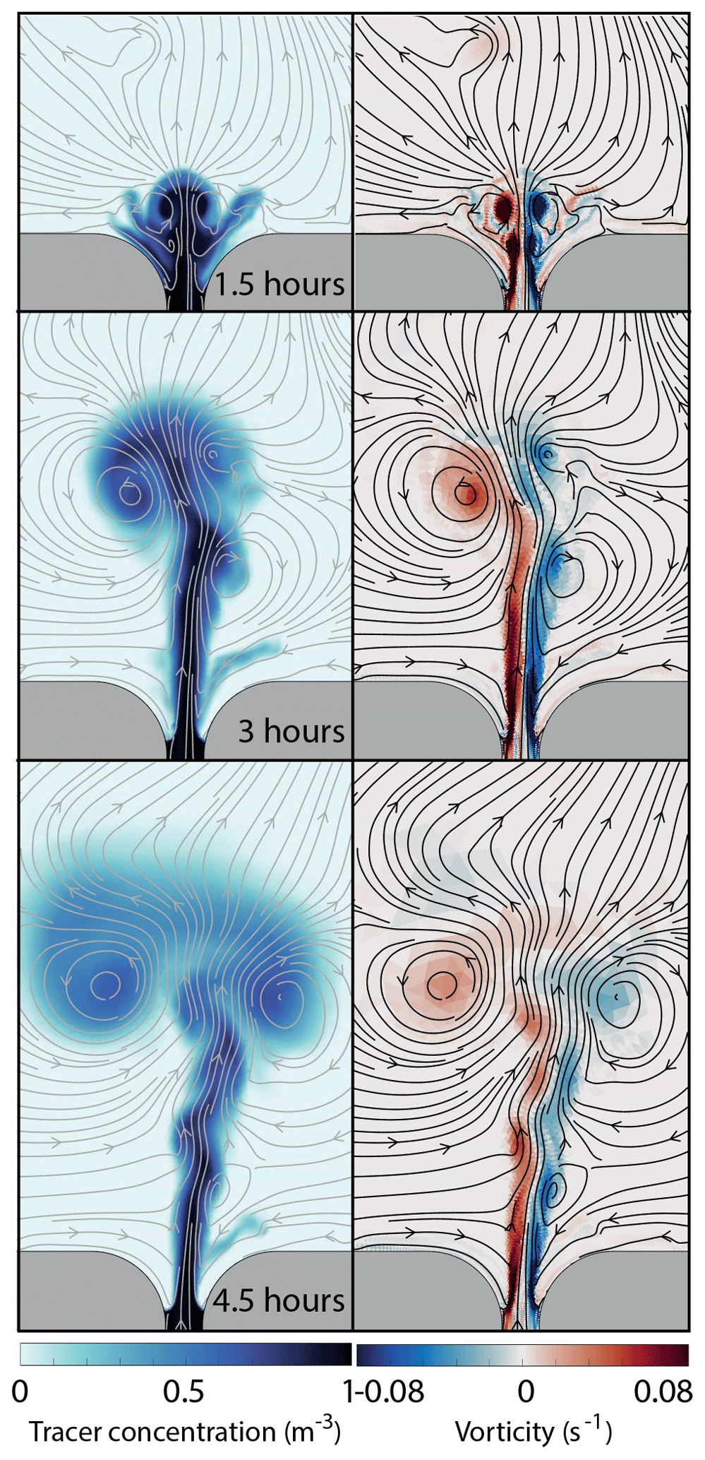
Figure 5 The temporal tracer and vorticity fields, with the corresponding stream function, are displayed for a 1 km wide and 4 km long strait in the left and right panel, respectively. The experiment is forced with a tidal wave of amplitude A_t=1 m. The upper, middle, and lower panels show a snapshot in time of the tracer and the vorticity fields at 1.5, 3, and 4.5 h after slack tide, respectively.

We choose to show three examples in which the tidal forcing and the strait length are equal (A_t=1 m and L=4 km), and the strait widths are W=1, W=4.5, and W=12 km. The difference in strait width results in different temporal evolution of the tracer distribution and the vorticity fields. We show the results from the first half of the tidal cycle, which we define to start at slack tide after ebb. The first 6 h (t=0–6 h) are during flood tide and the tidal current is directed northward. All three examples have flow separation and vortex formation at the strait exit, but only in the two former do the vortices connect into self-propagating dipoles.

In the narrowest strait (W=1 km, Fig. 5), the flow separates and vortices form 1.5 h after slack tide. At this point the flow is dominated by two separated shear layers with negative (right) and positive (left) vorticity. The separated shear layers are connected via a trailing jet to the two initial vortices, which now form a self-propagating dipole. The dipole at this stage consists of two intense vortex cores filled with water having a tracer concentration near 1. After 3 h, the dipole has increased in size and the vortex cores are somewhat less intense. The outer part of the dipole now consists of water with nearly zero vorticity and a nearly zero tracer concentration. The streamlines indicate that this low-concentration water has not come through the strait but is entrained into the dipole at the northern side of the strait. The dipole continues to grow while moving northward, fed by the trailing jet and by entrainment of low-vorticity water. Since the dipole is formed early in the tidal cycle, the dipole has time to propagate far northward before the flow reverses.

In the 4.5 km wide strait (Fig. 6) the time period from slack tide until flow separation and dipole formation is longer than in the 1 km wide strait. At 1.5 h separation has not yet occurred. The vorticity is confined to the narrow viscous boundary layers, while the tracer has started to exit the strait. The width of the two boundary layers is similar to the 1 km strait. However, since the strait is wider, the boundary layers occupy a smaller fraction of the strait. Most of the water flowing through the strait therefore has nearly zero vorticity. At 3 h, a dipole has formed and grows while moving northward during the tidal period. The vorticity is mainly located inside the vortex cores and most of the dipole consists of water with nearly zero vorticity. An obvious difference from the 1 km wide strait (Fig. 5) is that much of the nearly zero-vorticity water in the dipole has come through the strait and contains tracer. This leads to a pattern with the tracer covering a larger area than the vorticity. The dipole barley detaches from the coastline before the flow reverses, and no proper trailing jet is formed. Instead, we observe a continuous vortex shedding from the separated shear layer at the strait exit, which to some degree interacts and merges with the stronger initial vortices.

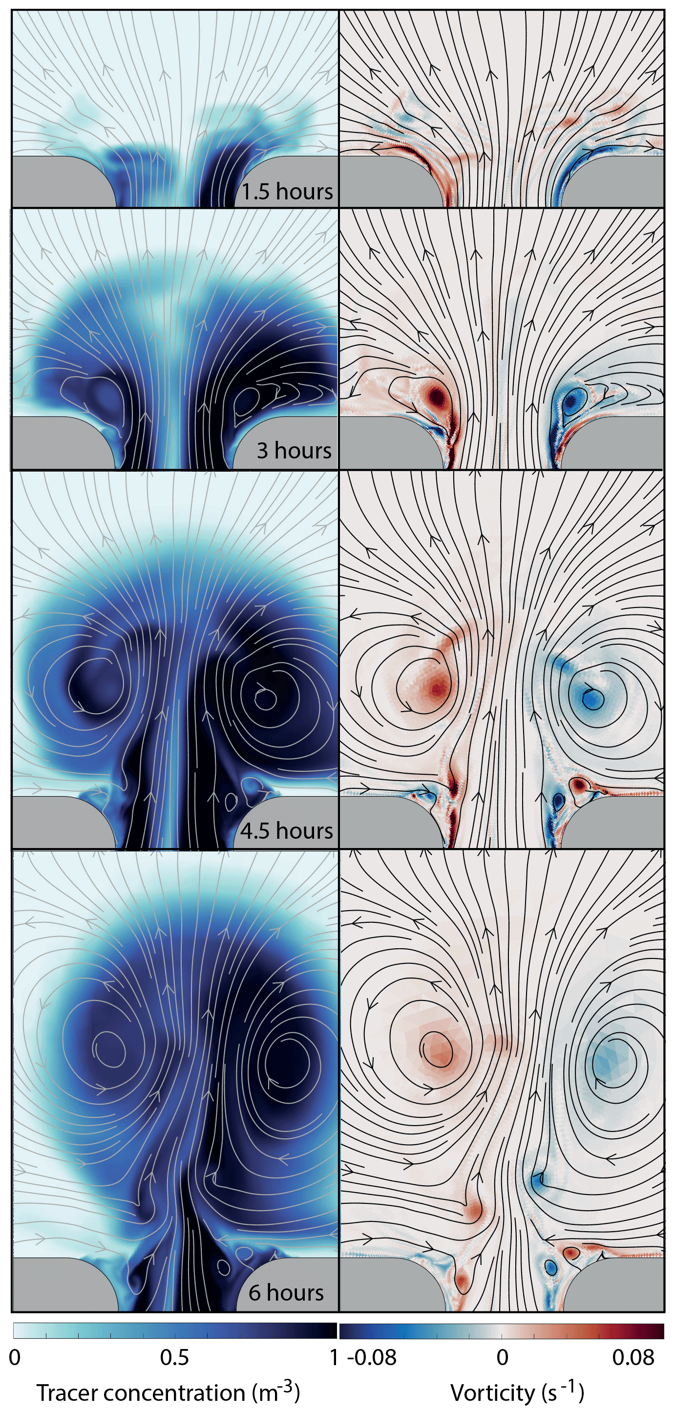
Figure 6 The temporal tracer and vorticity fields, with the corresponding stream function, are displayed for a 4.5 km wide and 4 km long strait in the left and right panel, respectively. The experiment is forced with a tidal wave of amplitude A_t=1 m. The upper, middle, and lower panels show a snapshot in time of the tracer and the vorticity fields at 1.5, 3, and 4.5 h after slack tide, respectively.

In the widest strait (W=12 km) we observe a continuous vortex shedding from the boundary layer, similar to the 4.5 km wide strait (Fig. 7). However, the vortices never interact across the width of the strait to form a dipole. In addition to a larger separation distance between the counter-rotating vortices, the flow also separates later than in the two former examples. The first vortices observed at the exit, 3 h after slack tide, are advected through the strait and not formed at the northern exit during the ongoing tidal phase. After almost 4 h, the first vortices are shed from the separated boundary layer. These vortices do not interact across the strait to form a dipole, but rather seem to interact and merge with other co-rotating vortices at the same side of the strait. Since no self-propagating dipoles are formed, the vortices do not escape the return flow and the net tracer transport through the strait is nearly zero.

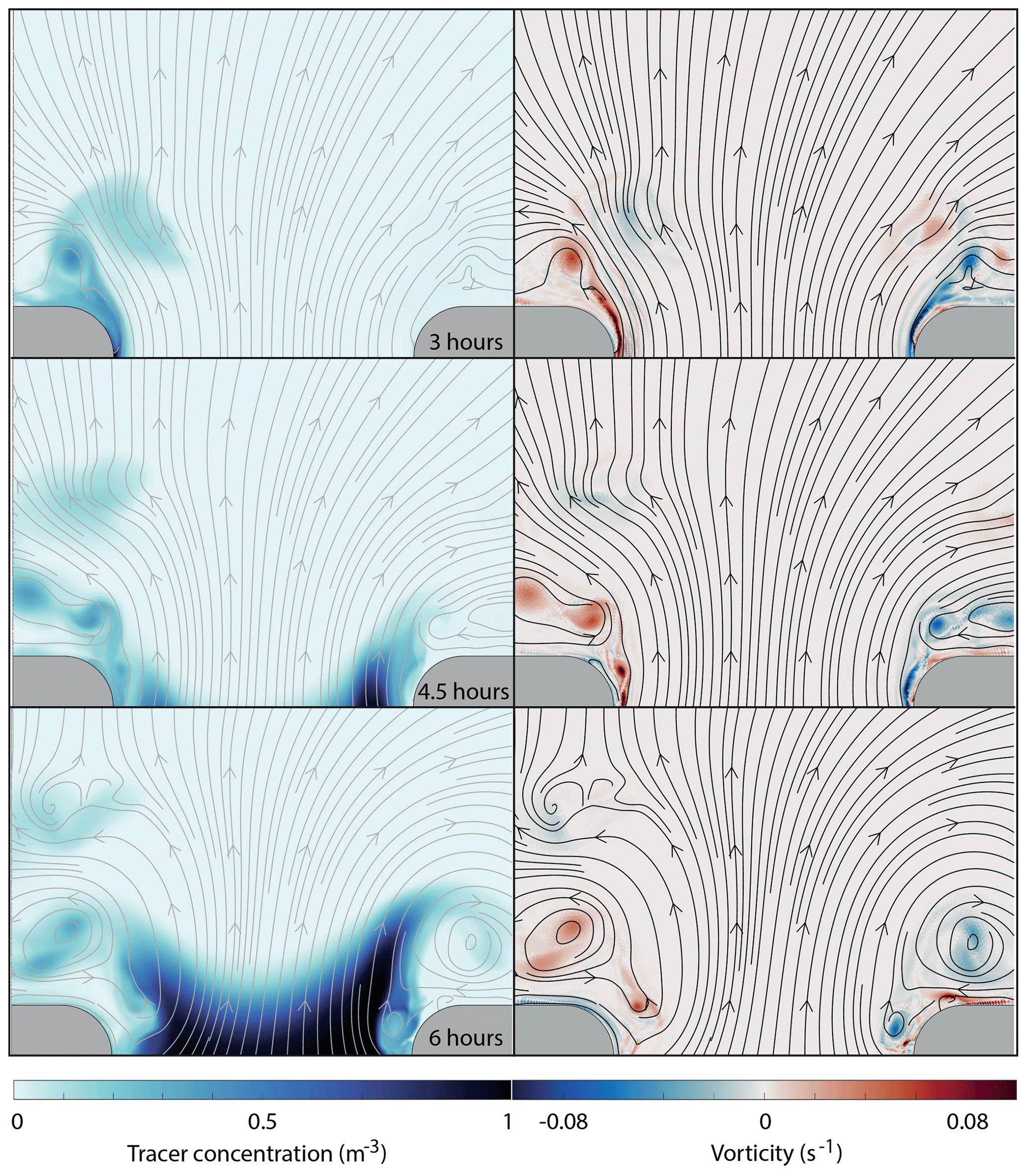
Figure 7 The temporal tracer and vorticity fields, with the corresponding stream function, are displayed for a 12 km wide and 4 km long strait in the left and right panel, respectively. The experiment is forced with a tidal wave of amplitude A_t=1 m. The upper, middle, and lower panels show a snapshot in time of the tracer and the vorticity fields at 1.5, 3, and 4.5 h after slack tide, respectively.

The three examples shown in Figs. 5 to 7 all have the same channel length, but they illustrate the process of dipole formation and dipole transport properties. These processes are similar for all channel lengths, although the channel length influences channel flow and thereby whether dipoles form or not. In general, longer straits require narrower strait widths for dipoles to form (Fig. 4), and flow separation and vortex formation occur later in the tidal cycle.

In the following, we go into the details of flow separation, vortex formation, and dipole properties. These topics are important for the understanding of how strait geometry affects flow dynamics and water exchange through narrow tidal straits.

4 Flow separation and vortex formation

The timing of flow separation depends on the flow dynamics at the strait exit. Here the balance between nonlinear advection and pressure forces leads to an adverse pressure gradient caused by the widening of the strait. The flow separates from the coastline when the adverse pressure gradient acts in the same direction as the friction and brings the velocity in the viscous boundary layer to zero (Signell and Geyer, 1991; Kundu, 1990). Since the adverse pressure gradient results from the nonlinear advection, the separation time can be related to the ratio of local acceleration to nonlinear advection, also called the Keulegan–Carpenter number (K_c) (Signell and Geyer, 1991). Flow separation can occur when

$$\begin{array}{}\text{(10)}& K_{\mathrm{c}}={\displaystyle \frac{U{T}^{*}}{R}}>\mathrm{1},\end{array}$$

where T^* is the timescale over which the flow dynamics become nonlinear and R is the length scale of the strait exit (Fig. 3b). From here and through the rest of the paper, the velocity scale U is given by the tidal velocity amplitude. This is calculated as the maximum in time of the cross-strait average at y=y_u (see Fig. 3 for coordinate definitions). Assuming the time of separation, T_s, can be related to T^* and that K_c must obtain a certain value for separation to occur, then T_s should be proportional to $R/U$. This relation is confirmed when plotting T_s against $R/U$ (see Fig. 8). Here, T_s is the separation time obtained from the model results (details of how T_s is obtained are given below). Corresponding values of K_c lay mainly between 5 and 15.

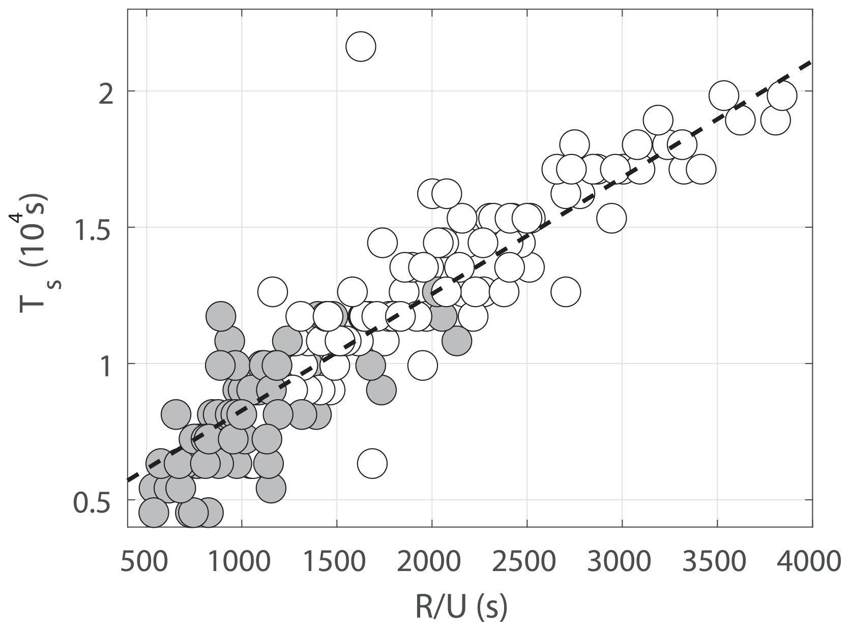
Figure 8 Separation time (T_s) plotted against $R/U$. The dashed line is the best linear fit $T_{\mathrm{s}}=\mathrm{4.3}R/U+\mathrm{3998}$. Straits with self-propagating dipoles are marked in gray.

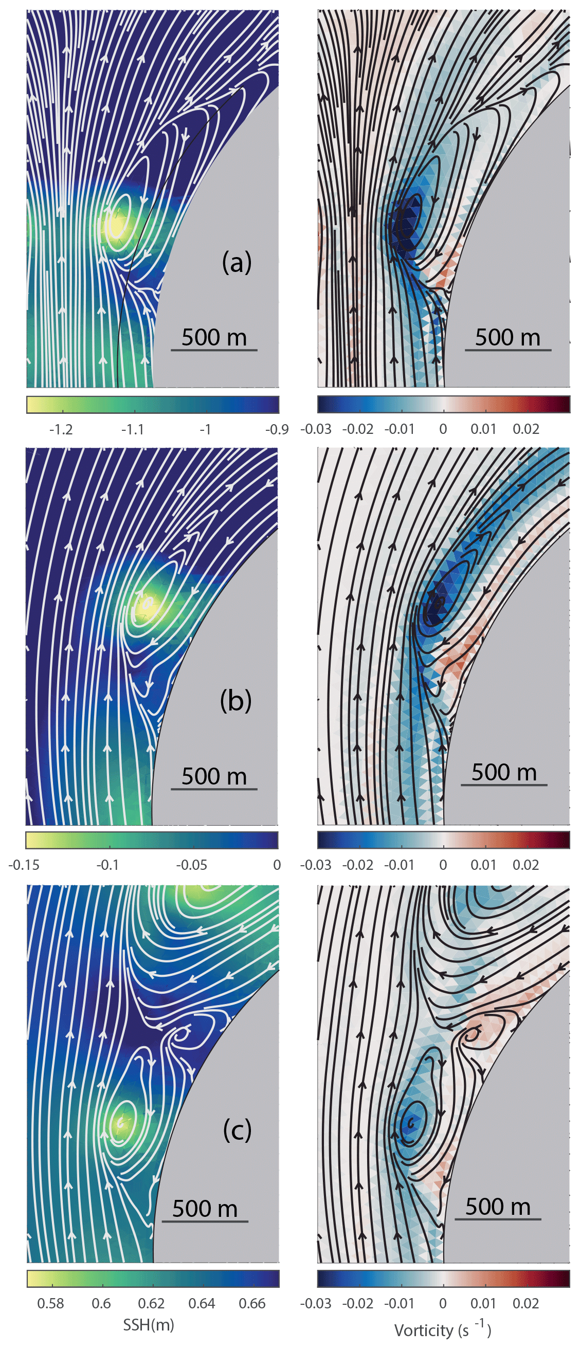
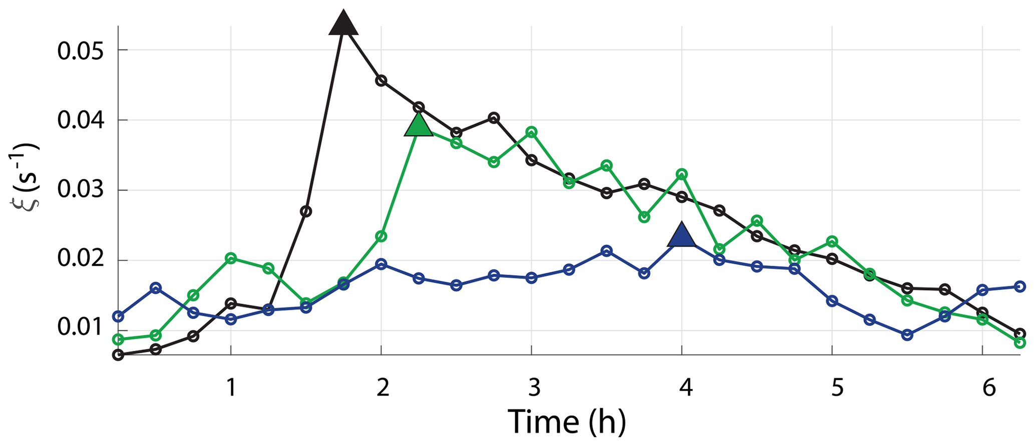
The formation of starting vortices and self-propagating dipoles occurs when the flow separates. The vorticity needed to form these vortices originates from the strong velocity front that is formed at the boundary between the newly separated flow and the reversed flow along the coast. At the time of flow separation, the velocity front immediately rolls up into a vortex. This process is illustrated in Fig. 9, where the flow field near the point of separation is plotted on top of vorticity and surface elevation for the same three simulations shown in Figs. 5 to 7. The vorticity created in the velocity front causes a maximum absolute value of vorticity to occur at separation time. This is shown in Fig. 10 for the same three simulations shown in Fig. 9.

For the simulations with strait widths of 1 and 4.5 km (upper and middle panels of Fig. 9) the two initial vortices interact and form a dipole. In these two straits we see a rapid buildup towards the maximum absolute value in vorticity followed by a decrease (black and green curve in Fig. 10). In the 1 km wide strait the initial vortices remain attached to the strait by a trailing jet, and we observe only one prominent peak in maximum absolute value of vorticity (black curve in Fig. 10). In the 4.5 km wide strait several vortices are shed from the separated velocity front after the initial vortex shedding (see Fig. 6), and several local maximums occur after flow separation (green curve in Fig. 10). In the widest strait the initial vortices never connect into a dipole, and the maximum absolute value of vorticity is much less prominent compared to the narrower straits (blue curve in Fig. 10). However, for the widest strait we also observe by visual inspection that the maximum absolute value of vorticity coincides with the initial vortex formation due to flow separation at about 4 h after slack tide. We find that, for all simulations, the maximum absolute value of vorticity corresponds to the separation time. Therefore, the separation time is estimated from the timing of the absolute value of vorticity within the strait exit ($y_u<y\le y_{\mathrm{e}}$, see Fig. 3b).

Figure 9 Sea surface height (left) and vorticity (right), with contours showing the corresponding streamlines, are shown at separation time. We show the fields in the three straits displayed in (a) Fig. 5 (W=1 km), (b) Fig.6 (W=4.5 km), and (c) Fig. 7 (W=12 km).

Figure 10 Time series of the maximum magnitude of vorticity at the strait exit, defined as the area where $y_u<y\le y_{\mathrm{e}}$. The black, green, and blue curves represents the same three simulations shown in Figs. 5 to 7, respectively. The triangles mark the separation time.

The initial vorticity of the vortices created during flow separation is an important parameter for determining their ability to form a dipole and the propagation velocity of the dipole that forms. Here, the vortices are represented by the radial profiles of Lamb–Oseen (LO) vortices (Lamb, 1916; Leweke et al., 2016):

$$\begin{array}{}\text{(11a)}& {\displaystyle }& {\displaystyle }{v}_{\mathit{\theta }}={\displaystyle \frac{\mathrm{\Gamma }}{\mathrm{2}\mathit{\pi }r}}\left(\mathrm{1}-e^{-\frac{r^{\mathrm{2}}}{a^{\mathrm{2}}}}\right),\text{(11b)}& {\displaystyle }& {\displaystyle }\mathit{\xi }={\displaystyle \frac{\mathrm{\Gamma }}{\mathit{\pi }{a}^{\mathrm{2}}}}{e}^{-\frac{r^{\mathrm{2}}}{a^{\mathrm{2}}}},\end{array}$$

where ξ is the vorticity, Γ is the circulation of the vortex, a is the radius of the vortex core, and r is the distance from the center of the vortex core. Originally, a increases with time and depends on viscosity. Equation (11b) is a particular solution to the Navier–Stokes equations (Habibah et al., 2018) and is known to show good agreement with experimental data (Leweke et al., 2016). The vortex shape described by Eq. (11b) fits our modeled vorticity well (see Fig. 11). We obtain the core radius a by finding the best fit of Eq. (11b) to the modeled vortices using the maximum and minimum vorticity from the model data.

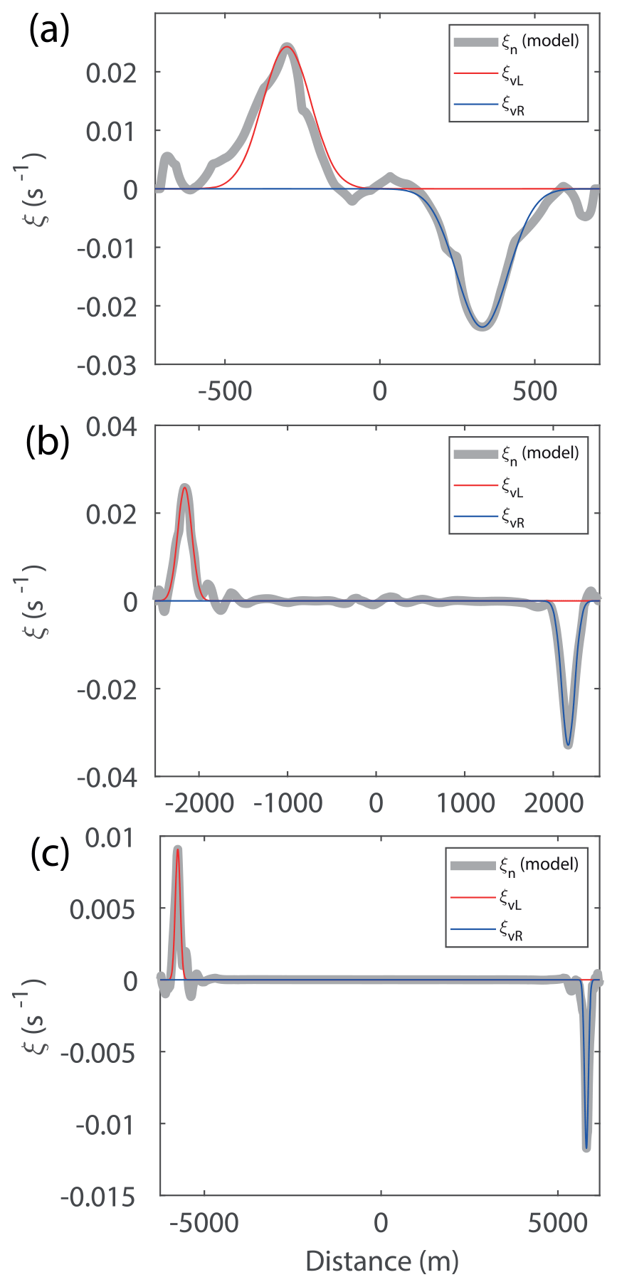
Figure 11 The vorticity distribution along a line intersecting the two vortices at each side of the strait at separation time. Panels (a–c) are from the three simulations shown in Figs. 5 to 7, respectively. The gray line shows the vorticity distribution from the model output, while the red and blue lines are calculated vorticity distribution using Eq. (11b) for the left and right vortex, respectively.

From the results shown in Fig. 9 we see that the newly formed vortices have nearly equal size, even though the three simulations have very different characteristics. The estimation of core radius for all 164 simulations shows that what is indicated by Fig. 9 is a general result. The estimated core radius at separation time is given by $a\left(T_{\mathrm{s}}\right)=\mathrm{110}\pm \mathrm{18}$ m for all simulations and $a\left(T_{\mathrm{s}}\right)=\mathrm{116}\pm \mathrm{14}$ m for the dipoles (mean ± 1 standard deviation; see Fig. 12). This suggests that the vortex core radius is nearly constant across all simulations, which again suggests that the vorticity should be proportional to the strait velocity. Plotting the maximum absolute value of vorticity against the along-strait velocity at separation time v(T_s) (Fig. 13) suggests that the maximum absolute value of vorticity can be represented as

$$\begin{array}{}\text{(12)}& {\left|\mathit{\xi }\left(T_{\mathrm{s}}\right)\right|}_{\max }\simeq {\displaystyle \frac{\left|v\left(T_{\mathrm{s}}\right)\right|}{a\left(T_{\mathrm{s}}\right)}}.\end{array}$$

It must be kept in mind that the simulated values of vorticity are strongly dependent on resolution. However, the important point is that vorticity can be expressed as shown in Eq. (12) and Fig. 13, which is likely to also be true for higher-resolution simulations with higher maximum vorticity. The effect of resolution will be discussed in more detail in Sect. 8.1.

Figure 12 The vortex core radius at separation time plotted against the separation time. The core radius is the mean radius of the two vortex cores formed at each side of the strait. Straits with self-propagating dipoles are marked in gray.

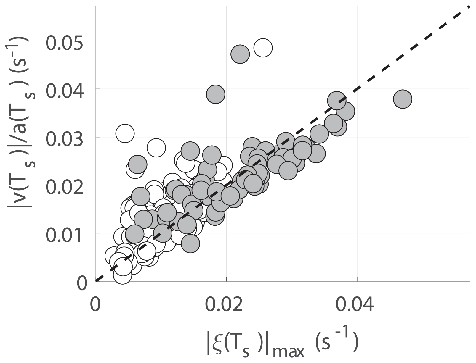
Figure 13 The theoretical velocity shear $v/a$ plotted against the absolute value of the vorticity in the vortices at separation time. Straits with self-propagating dipoles are marked in gray.

We have shown that the flow separation coincides with a maximum in absolute value of vorticity and that the dipole is formed at the time of separation. The vorticity of the initial vortices is given by strait velocity divided by the core radius, and the initial core radius is nearly equal for all simulations. In the following section, we describe how dipole vortices are recognized and the determination of their propagation velocity.

5 Dipole recognition and tracking

To obtain dipole properties we track the initial vortices from the time of flow separation to the end of the tidal phase. The vortex centers are points of minimum surface elevation as seen in Fig. 9. So, when tracking the vortices, we simply track the minima in surface elevation. Typically, vortices form simultaneously on each side of the strait at separation time, and we start tracking the two minima in surface elevation from this moment. We evaluate the propagation velocity and direction of the two vortices to determine whether they have connected into a dipole or not using two criteria illustrated in Fig. 14.

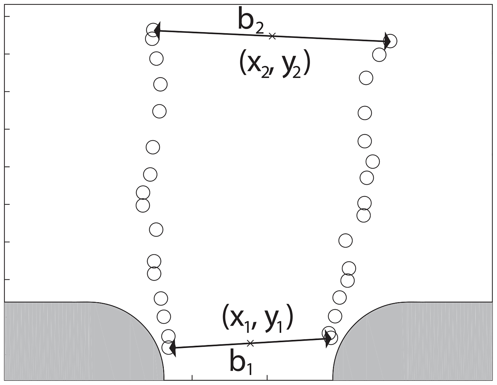
Figure 14 A sketch illustrating the dipole tracking. (x₁, y₁) represents the position of the midpoint between the two vortices, and b₁ is the distance between the two vortices at separation time, t=T_s. Likewise, (x₂, y₂) represents the position on the midpoint between the vortices, and b₂ is the distance between the vortices at $t=T_{\mathrm{s}}+\mathrm{\Delta }t$.

The criteria are based on two simple principles. The first criterion is that a dipole will propagate normal to the line connecting the two vortices and therefore conserve the distance between them (Leweke et al., 2016). We observe that vortices that do not connect into dipoles tend to be advected to each side of the strait opening, increasing the distance between them. The second criterion is based on the fact that a dipole escaping the returning tidal flow needs to have a propagating velocity over a certain limit. Fitting these two criteria to the results of visual inspection leads to the following formulations used to recognize dipoles in the simulation results (see Fig. 14 for notations):

$$\begin{array}{}\text{(13)}& {\displaystyle \frac{b_{\mathrm{2}}-b_{\mathrm{1}}}{\mathrm{2}\left(y_{\mathrm{2}}-y_{\mathrm{1}}\right)}}<\mathrm{2.9}\end{array}$$

and

$$\begin{array}{}\text{(14)}& U_{\mathrm{dip}}={\displaystyle \frac{y_{\mathrm{2}}-y_{\mathrm{1}}}{\mathrm{\Delta }t}}>\mathrm{0.2}\mathrm{m}{\mathrm{s}}^{-\mathrm{1}}.\end{array}$$

The first of these criteria sets a limit to the increase in distance between the vortices compared to northward propagation of the dipole, while the second criterion requires that the dipole have a mean propagation speed larger than 0.2 m s⁻¹. Δt is the time between the two dipole positions given by y₁ and y₂. The last criterion is important to rule out dipoles that form late in the tidal cycle and will not escape the strait before the tidal current reverses. These dipoles often are too slow to move out of the strait, and their separation distance is therefore nearly constant because it is restricted by the coastline. To recognize escaping dipoles, we find that it is necessary to set a lower limit to their propagation velocity, and therefore we have introduced the second criterion defined by Eq. (14).

When tracking the vortices we obtain the dipole propagation velocities, which, together with the tidal velocity and vorticity distributions, enable us to investigate the vortex properties.

6 Representation of the dipole propagation velocity

Dipole properties, such as core radius (a) and propagation velocity (U_dip), determine the net water exchange through the strait (Kashiwai, 1984a; Wells and van Heijst, 2003). Another important parameter is the sink radius (R_s). The water volume within the semi-circle (sink region, Fig. 1a) with radius R_s will be drawn into the strait when the flow reverses at $t=T/\mathrm{2}$. If the dipole has traveled a distance larger than R_s it will escape the return flow. Here, we choose to investigate dipole properties inside the sink region.

Comparing the tracked dipole velocities to the theoretical velocities obtained from Eq. (1), we find that the dipole propagation velocity given by Eq. (1) is too low. Instead, we get a much better fit when using the sum of the contributions from the two vortices,

$$\begin{array}{}\text{(15)}& U_{\mathrm{dip}}\simeq {\displaystyle \frac{\left|{\mathrm{\Gamma }}_{\mathrm{1}}\right|+\left|{\mathrm{\Gamma }}_{\mathrm{2}}\right|}{\mathrm{2}\mathit{\pi }b}},\end{array}$$

where Γ₁ and Γ₂ are the circulations of the two vortices. We calculate Γ₁ and Γ₂ from Eq. (11b) using the value of maximum vorticity,

$$\begin{array}{}\text{(16)}& \mathrm{\Gamma }=\mathit{\pi }{a}^{\mathrm{2}}{\mathit{\xi }}_{\max },\end{array}$$

and compare the dipole propagation velocity estimated using Eq. (15) to the tracked velocities. Figure 15 shows the comparison for each time step in the same two simulations shown in Figs. 5 and 6, and Fig. 16a shows the comparison for dipole velocities averaged within the sink region.

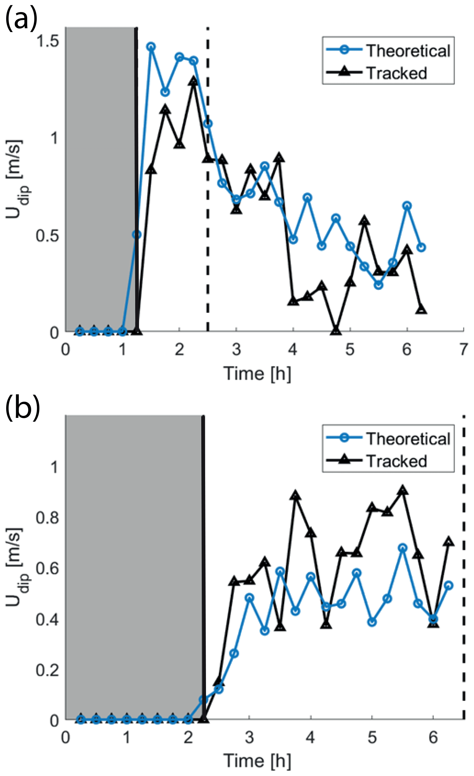
Figure 15 Dipole propagation velocity for a dipole formed in (a) the 1 km wide and 4 km long strait shown in Fig. 5, as well as (b) the 4.5 km wide and 4 km long strait shown in Fig. 6. The black curves are velocities obtained from dipole tracking, while the blue curves are velocities calculated using Eq. (15). The gray patch indicates the time before flow separation. The dashed black line indicates when the dipole escapes the sink region.

Figure 16 The dipole velocities obtained from tracking (on the x axis) plotted against (a) the theoretical dipole velocities (Eq. 15) and against Uα (Eq. 18) in the lower panel. The tracked velocities, theoretical velocities, and α are averaged over the time period when the dipole is located inside the sink region.

Assuming the two vortices are of equal strength gives

$$\begin{array}{}\text{(17)}& U_{\mathrm{dip}}\simeq {\displaystyle \frac{\mathrm{\Gamma }}{\mathit{\pi }b}}.\end{array}$$

Since the majority of the vorticity is contained within the core radius, scale analysis gives Γ≃πaU, which is obtained by assuming $\mathit{\xi }\simeq U/a$. This suggests that the dipole propagation velocity can be represented as

$$\begin{array}{}\text{(18)}& U_{\mathrm{dip}}\simeq \mathit{\alpha }U,\end{array}$$

where $\mathit{\alpha }=a/b$ is the aspect ratio of the vortices. The comparison to tracked velocities (Fig. 16b) shows that Eq. (18) is a good representation of the dipole propagation velocity.

The dipole propagation velocity is crucial when determining the transport properties of the dipole in relation to tidal pumping (Kashiwai, 1984a; Wells and van Heijst, 2003). In the next section we will use the simple relations found here in the search for a parameter describing the net water exchange through the strait.

7 Water exchange through the strait

7.1 Effective tracer transport

To investigate the role of dipole vortices in generating net water exchange, we first quantify the effective tracer transport Q_e:

$$\begin{array}{}\text{(19)}& Q_{\mathrm{e}}={\displaystyle \frac{Q_{\mathrm{n}}}{Q_{\mathrm{m}}}}.\end{array}$$

Q_e is the ratio between the net tracer transport Q_n and the maximum potential for net tracer transport through the strait Q_m over the course of one tidal cycle. Q_n is calculated through a cross section in the center of the strait ($y=y_{\mathrm{e}}-L/\mathrm{2}$) as

$$\begin{array}{}\text{(20)}& Q_{\mathrm{n}}=\sum _{t=\mathrm{0}}^T\sum _{n=\mathrm{1}}^N{c}_{\mathrm{n}}{v}_{\mathrm{n}}\mathrm{d}{A}_{\mathrm{n}}\mathrm{d}t.\end{array}$$

Here v_n is the normal velocity through an area element dA_n, and c_n is the tracer concentration in grid cell n. Q_m is given by

$$\begin{array}{}\text{(21)}& Q_{\mathrm{m}}=\sum _{t=\mathrm{0}}^{T/\mathrm{2}}\sum _{n=\mathrm{1}}^N{c}_{\max }{v}_{\mathrm{n}}\mathrm{d}{A}_{\mathrm{n}}\mathrm{d}t+\sum _{t=T/\mathrm{2}}^T\sum _{n=\mathrm{1}}^N{c}_{\min }{v}_{\mathrm{n}}\mathrm{d}{A}_{\mathrm{n}}\mathrm{d}t.\end{array}$$

The maximum possible tracer transport occurs when the northward transport consists entirely of water containing tracer concentration c=c_max, and the southward transport consists entirely of water containing tracer concentration c=c_min. In our case c_max=1 m⁻³ and c_min=0 m⁻³. The effective tracer transport is independent of the volume transport and is a measure of how efficiently water is exchanged through the strait.

7.2 Water exchange by self-propagating dipoles

The ability of the dipole to escape the return flow determines its contribution to water exchange through a strait (Kashiwai, 1984a; Wells and van Heijst, 2003). Both Kashiwai (1984a) and Wells and van Heijst (2003) investigated the dipole position relative to the sink region at flow reversal to evaluate the ability of the dipole to escape. While Kashiwai (1984a) only considered the position of the dipole relative to the sink region, Wells and van Heijst (2003) evaluated the strength of the return flow relative to the dipole velocity at its position. Both approaches resulted in a threshold value of the Strouhal number (St_c) between 0.8 and 0.13, separating the dipoles escaping (St<St_c) and dipoles not escaping (St>St_c) the return flow.

We follow the approach of Kashiwai (1984a) and investigate the dipole transport potential by evaluating the dipole propagation distance, L_d, relative to the sink radius, R_s, at $t=T/\mathrm{2}$.

$$\begin{array}{}\text{(22)}& L_{\mathrm{d}}=U_{\mathrm{dip}}\left({\displaystyle \frac{T}{\mathrm{2}}}-T_{\mathrm{s}}\right),\end{array}$$

and R_s is given by

$$\begin{array}{}\text{(23)}& R_{\mathrm{s}}=\sqrt{{\displaystyle \frac{\mathrm{2}Q}{\mathit{\pi }H}}}={\displaystyle \frac{\sqrt{\mathrm{2}WUT}}{\mathit{\pi }}},\end{array}$$

where W is channel width, $Q\simeq WH\underset{\mathrm{0}}{\overset{T/\mathrm{2}}{\int }}v\mathrm{d}t=WHUT/\mathit{\pi }$ is the tidal prism, and v=Usin (ωt) is the along-strait velocity. Here we assume the sink region is formed as a semi-circle with a radius R_s, and the water depth H is constant inside the domain.

The position of the dipole relative to the sink radius at $t=T/\mathrm{2}$ is evaluated by the nondimensional parameter S_d:

$$\begin{array}{}\text{(24)}& S_{\mathrm{d}}={\displaystyle \frac{R_{\mathrm{s}}}{L_{\mathrm{d}}}}={\displaystyle \frac{\sqrt{\mathrm{2}WUT}}{\mathit{\pi }{U}_{\mathrm{dip}}\left(\frac{T}{\mathrm{2}}-T_{\mathrm{s}}\right)}}.\end{array}$$

This expression is formulated in the same fashion as the Strouhal number by Kashiwai (1984a) and Wells and van Heijst (2003), meaning that low numbers favor escaping dipoles and effective water exchange. If S_d>1 the dipole is inside the sink region when the flow reverses, and conversely, if S_d<1 the dipole is outside the sink region and will escape the return flow. S_d considers dipole transport properties only and shows different behavior for the different strait lengths when plotted against effective tracer transport (Fig. 17a). Values of S_d well below 1 do not guarantee net tracer transport, as can be seen for some of the longest straits (Fig. 17a). This indicates that we need to consider the strait length in order to describe the effective tracer transport through the strait.

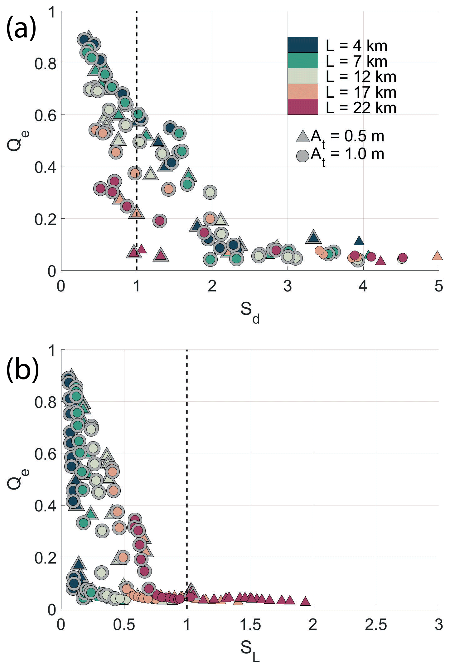
Figure 17 The effective transport, Q_e, plotted against the nondimensional parameters (a) S_d and (b) S_L. Dipoles, recognized from the criteria given in Sect. 5, are marked with a gray halo.

The dipole can only be an important contributor for water exchange if the strait is shorter than the tidal excursion. If the strait is longer than the tidal excursion, the water mass on one side of the strait will not be able to travel through the strait, with zero net tracer exchange as a result. In order to evaluate the effect of strait length we introduce the nondimensional length scale as

$$\begin{array}{}\text{(25)}& S_{\mathrm{L}}={\displaystyle \frac{L}{L_{\mathrm{t}}}}={\displaystyle \frac{\mathit{\pi }L}{U_{\mathrm{m}}T}}.\end{array}$$

Here, $L_{\mathrm{t}}=\underset{\mathrm{0}}{\overset{T/\mathrm{2}}{\int }}{v}_{\mathrm{m}}\mathrm{d}t$ is the tidal excursion and L is the strait length. v_m=U_msin (ωt) is the cross-strait maximum tidal current, and U_m is the amplitude of v_m. We choose to use the maximum current in the estimation of L_t because this ensures that the net tracer transport is zero for S_L>1. In this case the tracer front will not propagate through the strait during one-half tidal cycle and no tracer will be available for the dipole to capture and transport away from the strait. This is the case for many of the long straits, with zero tracer transport as a result (Fig. 17b). However, similarly as for S_d, S_L<1 does not guarantee a net tracer transport.

S_L and S_d can be combined to give the effective tracer transport through the strait. To show this we consider the situation in which S_L<1, which ensures that tracer will flow through the channel. We apply a simple kinematic model illustrated by Fig. 18. This figure shows the tracer distribution at $t=T/\mathrm{2}$; the dark gray represents the tracer in the dipole, the medium gray represents the tracer in the jet following the dipole, and the light gray is the tracer inside the channel. All the tracer inside the channel and an unknown fraction of the tracer in the jet and dipole will be drawn back into the channel when the flow turns at $t=T/\mathrm{2}$. We assume that the fraction inside the sink region will be drawn back, but this fraction depends on the shape of the dipole and jet, which is not easily estimated. However, to simplify the problem we assume that the dipole or jet is shaped like a rectangle, as illustrated by the green box in Fig. 18. The fraction inside R_s is now given by the lengths L_d, R_s, and r_d only. We have introduced the distance r_d to include the fact that parts of the dipole can escape even if L_d<R_s.

Figure 18 Idealized distribution of a tracer at $t=T/\mathrm{2}$ between the dipole (dark gray), jet (medium gray), and strait (light gray).

At t=0 we assume that the tracer front is located on one side of the strait at y=y₀ and that the water transported into the strait at y=y₀ always has a tracer concentration equal to c_max. The tracer transported through the cross section at y=y₀ between t=0 and $t=T/\mathrm{2}$ is given by c_maxWHL_t. The tracer distribution at $t=T/\mathrm{2}$ is divided between the strait, jet, and dipole as illustrated in Fig. 18. This can be expressed as

$$\begin{array}{}\text{(26)}& W{L}_{\mathrm{t}}=WL+W{L}_{\mathrm{d}}+V_{\mathrm{dip}},\end{array}$$

where V_dip represents the volume with tracer concentrations equal to c_max in the dipole. H and c_max cancel since they appear on both sides of the equation. If the water that is drawn back maintains its tracer concentration c_max and the water that originates on the other side of the strait has a tracer concentration of c_min, the net tracer transport can be expressed as

$$\begin{array}{}\text{(27)}& \begin{array}{rl}{q}_{\mathrm{n}}& =\left(W\left(L_{\mathrm{t}}-L\right)-{\displaystyle \frac{R_{\mathrm{s}}}{L_{\mathrm{d}}+r_{\mathrm{d}}}}\left(W{L}_{\mathrm{d}}{V}_{\mathrm{dip}}\right)\right)c_{\max }\\ & -{\displaystyle \frac{L_{\mathrm{d}}+r_{\mathrm{d}}-R_{\mathrm{s}}}{L_{\mathrm{d}}+r}}\left(W{L}_{\mathrm{d}}+V_{\mathrm{dip}}\right)c_{\min }.\end{array}\end{array}$$

Here, we assume that the net volume flux during one tidal cycle is zero. Combining Eqs. (26) and (27) gives

$$\begin{array}{}\text{(28)}& q_{\mathrm{n}}=W\left(L_{\mathrm{t}}-L\right)\left(\mathrm{1}-{\displaystyle \frac{R_{\mathrm{s}}}{L_{\mathrm{d}}+r_{\mathrm{d}}}}\right)\left(c_{\max }-c_{\min }\right).\end{array}$$

The maximum potential for tracer transport (see Eq. 21) is

$$\begin{array}{}\text{(29)}& q_{\mathrm{m}}=W{L}_{\mathrm{t}}\left(c_{\max }-c_{\min }\right).\end{array}$$

Dividing Eq. (28) by q_m gives the effective tracer transport as

$$\begin{array}{}\text{(30)}& q_{\mathrm{e}}=\left(\mathrm{1}-S_{\mathrm{L}}\right)\left(\mathrm{1}-{\displaystyle \frac{S_{\mathrm{d}}}{X_{\mathrm{d}}}}\right),\end{array}$$

where X_d is given by

$$\begin{array}{}\text{(31)}& X_{\mathrm{d}}=\mathrm{1}+{\displaystyle \frac{r_{\mathrm{d}}}{L_{\mathrm{d}}}}.\end{array}$$

Thus, using the simple kinematic model (Fig. 18), we can express the effective tracer transport in a simple combination of S_d and S_L, as well as the new parameter X_d. The result is shown in Fig. 19, where we plot q_e against Q_e for two different values of X_d. It is clear that X_d, which represents the size of the dipole, is vital to get a good fit between the kinematic model (Fig. 18) and the simulation results. For X_d=1 (Fig. 19a), corresponding to r_d=0, the fit between simulation results and the kinematic model is not very good, although the kinematic model captures the main physics. However, using X_d=1.67 collects the simulation results tightly around the line Q_e=q_e (Fig. 19b).

Figure 19 The effective transport Q_e from the simulations (Eq. 19) plotted against the effective transport resulting from the simple kinematic model (Eq. 30) for (a) X_d=1 and (b) X_d=1.67. The dashed line indicates Q_e=q_e. Dipoles, recognized from the criteria given in Sect. 5, are marked with a gray halo.

8 Discussion

8.1 Sensitivity to mesh discretization

The resolution of our mesh varies from 50 m in the center of the strait to 20 km at the outer boundary. The Rossby radius is ∼230 km, and the northward-propagating Kelvin wave should therefore be well represented in the model. The mesh resolution is more critical in the center of the strait where vorticity and circulation are important parameters for vortex formation and dipole propagation. Vorticity is extremely sensitive to mesh resolution, and it is possible that the processes of separation and vortex formation are affected by the model resolution. In our case, the spatial scale of the initial vortices is close to the smallest scale the model can resolve. It is therefore important to investigate whether our conclusions regarding tracer transport, dipole propagation velocity, and separation time are affected by the model resolution.

Vorticity is created in the velocity front formed by flow separation. The simulated vorticity in the velocity front depends strongly on model resolution. However, the total production of vorticity with time is less dependent on resolution. This can be shown by integrating the vorticity over an area containing a segment of the velocity front. During a time t, a velocity front with length Ut is formed, where U is the tidal velocity in the strait. Assuming that the velocity equals U on one side of the front and zero on the other and that U is directed along the front gives (Kashiwai, 1984b)

$$\begin{array}{}\text{(32)}& \underset{A_{\mathrm{v}}}{\iint }\mathrm{\nabla }\times \mathit{v}\mathrm{d}A=\underset{C}{\oint }\mathit{v}\cdot \mathit{d}\mathit{l}\simeq U^{\mathrm{2}}t.\end{array}$$

Here A_v is the area enclosing a segment of the front, C is the closed contour encircling A_v, v is the velocity vector, and dl is an incremental length segment directed tangential to C. This result suggests that if the model resolution is sufficient to correctly represent the strait velocity and a flow separation, the total vorticity in a segment of the front is likely to be correct and independent of resolution. Since the vortices are formed from segments of the front, the total vorticity in the vortices and the circulation are likely to be similar between models of different resolution. Based on this analysis, we will argue that local vorticity is sensitive to mesh resolution, but the circulation is less sensitive to resolution as long as the model properly represents the strait velocity and a flow separation. Since dipole propagation velocity depends on the circulation of the vortices (Eq. 15), it is probably not very sensitive to mesh resolution.

To study the effect of resolution, we have repeated a number of the simulations using finer mesh resolution. In the new simulations, the resolution at the coast is set to 10 m inside the strait. The other simulations presented in this paper have 50 m resolution at the coastline (see Sect. 2.2). We have selected seven strait configurations which are simulated with higher resolution. These are the three simulations shown in Figs. 5 to 7 plus four others of different width and length. A comparison with the coarser simulations and final results for the simulations with 10 m resolution are shown in Fig. 20.

Figure 20 Comparison between 10 and 50 m resolution simulations. Panels (a–c) show the comparison in velocity scale U, dipole propagation velocity U_dip, and effective transport Q_e. Panels (d, e) show the effective transport Q_e (Eq. 19) from the finer-resolution simulations plotted against the effective transport resulting from the simple kinematic model (Eq. 30) for (d) X_d=1 and (e) X_d=1.67. The dashed line indicates Q_e=q_e. Dipoles, recognized from the criteria given in Sect. 5, are marked with a gray halo.

The strait velocities, dipole propagation velocities, and the effective transport resulting from the high-resolution simulations are all similar to the results from the coarser simulations (Fig. 20a–c), although dipole propagation velocities are slightly higher and effective transport is slightly lower for the new simulations. The effective transport shows similar agreement with results from the kinematic model (Fig. 20d and e) as the results from the 50 m resolution simulations (Fig. 19). The simulated effective transport fits the kinematic model results closely for X_d=1.67. This shows that mesh discretization has little influence on the main conclusions of this paper.

Even if the velocity, dipole propagation, and tracer transport are not very sensitive to mesh resolution, we clearly see that vorticity in the high-resolution simulations reaches larger values. Determining the separation time from the time of maximum vorticity is not a reliable method in the high-resolution simulations. There is still a significant vorticity increase at the time of separation, but the maximum vorticity now typically occurs at the time of maximum strait velocity. The separation times are therefore determined by visual inspection, and they are similar to the ones in the 50 m resolution simulations. Another interesting observation is that one side of the dipole may consist of two co-rotating vortices in the high-resolution simulations, while it is a single vortex in the coarser simulations. The theoretical dipole propagation velocity (Eq. 15) still fits the tracked velocity well if the circulation around both of the co-rotating vortices is considered.

8.2 Effect of strait length on flow dynamics

To understand why strait length is a restriction factor for dipole formation (Fig. 4), it is instructive to use the simplified model of Garrett and Cummins (2005). They consider the along-strait velocity v as a function of time and position y along the strait. The equation governing the flow is

$$\begin{array}{}\text{(33)}& {\displaystyle \frac{\partial v}{\partial t}}+v{\displaystyle \frac{\partial v}{\partial y}}=-g{\displaystyle \frac{\partial \mathit{\eta }}{\partial y}}-{\displaystyle \frac{C_{\mathrm{d}}}{H}}\left|v\right|v,\end{array}$$

where η is the surface elevation, C_d is the drag coefficient (Eq. 8), and H is depth. Scaling this equation using the velocity amplitude U as velocity scale, $T/\mathrm{2}$ as timescale, and the strait length L as length scale gives

$$\begin{array}{}\text{(34)}& \mathrm{2}{\displaystyle \frac{U}{T}}+{\displaystyle \frac{U^{\mathrm{2}}}{L}}\sim g{\displaystyle \frac{\mathit{\delta }\mathit{\eta }}{L}}-{\displaystyle \frac{C_{\mathrm{d}}}{H}}{U}^{\mathrm{2}},\end{array}$$

where δη is the surface elevation difference between the exit and entrance of the strait. Our model setup is designed such that the difference in surface elevation across the strait is set by the tidal wave propagating around the peninsula and not by the strait flow. Due to this, δη is treated as constant. From Eq. (34) it is clear that the pressure force and nonlinear acceleration terms decrease with strait length, while the linear acceleration and friction are both independent of length. For L<10 km, the nonlinear acceleration dominates the linear and frictional terms. When nonlinear acceleration dominates, this will balance the pressure term, which gives a velocity scale, $U\sim \sqrt{g\mathit{\delta }\mathit{\eta }}$. However, if either linear acceleration or friction balances the pressure force, the result is a velocity scale that decreases with length. Whether it is friction or linear acceleration that determines the length effect seen in Fig. 4 depends on the relation between these two terms. In our case, in which H=100 m, C_d∼0.001, and T∼45 000, the acceleration is about 4 times larger than the friction term for U=1 m s⁻¹. Therefore, it is mainly the linear acceleration that leads to the length effect seen in Fig. 4. For shallower depths it is likely that friction will cause a significant reduction in strait velocity. Smaller U requires narrower straits to obtain dipole formation, which explains the results shown in Fig. 4.

8.3 Dipole formation and flow separation

The dipole propagation velocity depends on the strength of the vortices set by their vorticity, and it is important to understand how the vorticity is generated. Wells and van Heijst (2003) assume that the vorticity is generated in the viscous boundary layer and injected into the vortices formed at the point of flow separation. Afanasyev (2006) introduces the “startup time”, which is the time when the dipole starts propagating after an initial growth period being fed by the jet. Our simulations show a somewhat different picture. The dipole starts moving as soon as it is formed, and we see no initial period of growth (Fig. 15). The dipole is formed at separation time (Fig. 9), and before this we see no sign of vortices in the vorticity field (e.g., upper panel in Fig. 6).

The dipole formation is associated with a maximum in time of the absolute value of vorticity (Fig. 10). In the high-resolution simulations presented in Sect. 8.1, flow separation does not occur at maximum vorticity but is still associated with a sharp increase in vorticity. This is an interesting phenomenon, and the question is whether the vorticity is a consequence of separation or if it plays an active role in causing the separation. Our results suggest that there is a buildup of vorticity before separation (Fig. 10), which indicates that the vorticity plays an active role in the separation process. The decrease in vorticity after separation might be connected to the roll-up of the velocity front creating the initial vortices. We see from our simulations that the core radius of the vortices increases and the maximum vorticity decreases with time. Assuming it would take time to build up the vorticity before another vortex is formed fits the picture of maximum absolute value of vorticity occurring at separation time. Buildup and shedding of vorticity are also observed to be important in controlling the separation point location of the flow around a wind turbine blade (Melius et al., 2018).

The velocity front rolls-up immediately after separation and creates the dipole vortices (Fig. 9). That the separated velocity front rolls up into a vortex is commonly observed in studies of flow separation (Délery, 2013), and that the velocity front is the origin of the vorticity was also proposed by Kashiwai (1984a, b). During a time T_* flow separation creates a velocity front of length UT_* and the velocity difference across the front is U. Using the same approach as in Eq. (32), we find that the circulation of the front is $\mathrm{\Gamma }\simeq U^{\mathrm{2}}{T}_{*}$ (Kashiwai, 1984b). Using this together with Eqs. (17) and (18), the timescale T_* can be expressed as

$$\begin{array}{}\text{(35)}& T_{*}={\displaystyle \frac{a\mathit{\pi }}{U}}.\end{array}$$

In our simulations, U varies between 1 and 4 m s⁻¹, and the initial core radius a is about 100 m for all simulations (Fig. 12). This gives a timescale T_* between 1 and 5 min. Thus, the initial vortices are created within 1 to 5 min after flow separation. Vorticity is also injected into the dipole after separation and the circulation in the dipole increases. However, the order of magnitude of the total increase in the circulation is roughly similar to the circulation in the initial vortices. Therefore, the circulation of the dipole is well below the maximum possible given by ${\mathrm{\Gamma }}_{\max }\approx U^{\mathrm{2}}\left(\frac{T}{\mathrm{2}}-T_{\mathrm{s}}\right)$, which occurs if all vorticity created in the separated velocity front is injected into the dipole.

8.4 Dipole propagation velocity

As shown by Figs. 15 and 16, Eq. (15) is a good representation of the dipole propagation velocity. However, Eq. (15) gives a velocity that is twice as large as estimates obtained using Eq. (1). The aspect ratio of our simulated dipoles is mostly small (α≪1) and the absolute maximum is about 0.5. For these aspect ratios Eq. (1) should be in good agreement with the simulated dipole velocities (Delbende and Rossi, 2009; Habibah et al., 2018), but instead the dipole propagation velocities are consistently twice as large. Recent work (Habibah et al., 2018) expresses the solution to the Navier–Stokes equation in the form of a power series in the aspect ratio. To first order the propagation velocity is given by our Eq. (1), and a correction to this only appears in the fifth order of the aspect ratio. In our case this correction should be small. Also, from Delbende and Rossi (2009) it appears that the propagation velocity actually decreases for increasing aspect ratio. Equation (1) gives the propagation velocity of a dipole moving in a nonmoving ocean with no external forces acting on the dipole. These approximations are probably not valid in a tidal strait, where a strong background flow is present and vorticity and momentum are injected into the dipole by the trailing jet. We suspect that this is the reason for the discrepancy between Eq. (1) and the tracked dipole velocities.

A derivation of propagation velocity for a dipole connected to a jet is presented by Afanasyev (2006). The budget of volume and momentum in the dipole leads to a propagation velocity equal to half the channel or jet velocity, in good agreement with observations. Afanasyev (2006) investigated a steady jet, but the mechanisms of momentum input from the jet to the dipole will apply also in our case of an oscillating tidal jet. We do not know the aspect ratio of the dipole studied by Afanasyev (2006), but it is not unlikely that it is around 0.5 and that his result is therefore in agreement with our result (Eq. 18). Equations (15) and (18) do not have a clear theoretical basis but show a good fit to our large ensemble of numerical simulations. Further studies of dipoles formed in tidal straits are needed to fully understand the propagation of these dipoles.

9 Summary and conclusion

In this study, we have performed a total of 164 numerical simulations of an ideal tidal strait, investigating flow separation, dipole formation, and water exchange for different widths and lengths of the strait. We show that dipoles form and start propagating at the time of flow separation. The vorticity of the dipole vortices originates from the velocity front created by flow separation. The simulated dipole propagation velocity is twice as large as the propagation velocity derived for vortex pairs with no background flow (Lamb, 1916; Delbende and Rossi, 2009; Habibah et al., 2018) (Eq. 1). This is probably caused by injection of momentum into the dipole by the tidal jet (Afanasyev, 2006).

We derive two parameters S_d and S_L. S_d (Eq. 24) is given by the ratio between sink radius and distance traveled by the dipole, while S_L (Eq. 25) is given by the ratio between strait length and tidal excursion. For S_L>1, the tracer will be contained within the strait through the whole tidal cycle and net transport is zero. For S_d>1, the center of the dipole will be inside the sink region when the flow turns at $t=T/\mathrm{2}$. However, since the dipole is of finite size a fraction of the dipole may still escape the return flow, causing net tracer transport. From a simple kinematic model we show that the effective tracer transport can be expressed by S_d, S_L, and a parameter X_d representing the dipole size relative to the sink region (Eqs. 30 and 31). $\mathrm{1}/X_{\mathrm{d}}$ acts as a weight to S_d. Setting the value of X_d such that effective transport is zero for values of the weighted S_d larger than 1 gives a remarkably good fit between the simple kinematic model and the numerical simulations (Fig. 19).

The kinematic model (Eq. 19) provides an understanding of the processes creating a net tracer transport through a tidal strait. In our idealized straits, the sink region is described by a half-circle, the coastline curvature at the strait exit is kept constant, and the strait is of uniform width. Along an irregular coast in the real world this will be different, but the physical processes will still be valid. An interesting continuation of this study will be to derive S_d, S_L, and X_d for a real coastline and investigate how well we can describe net tidal transport through straits.