the Creative Commons Attribution 4.0 License.
the Creative Commons Attribution 4.0 License.
 | 19 Jan 2021
A clustering-based approach to ocean model–data comparison around Antarctica
Christopher M. Little
Alice M. Barthel
Laurie Padman
The Antarctic Continental Shelf seas (ACSS) are a critical, rapidly changing element of the Earth system. Analyses of global-scale general circulation model (GCM) simulations, including those available through the Coupled Model Intercomparison Project, Phase 6 (CMIP6), can help reveal the origins of observed changes and predict the future evolution of the ACSS. However, an evaluation of ACSS hydrography in GCMs is vital: previous CMIP ensembles exhibit substantial mean-state biases (reflecting, for example, misplaced water masses) with a wide inter-model spread. Because the ACSS are also a sparely sampled region, grid-point-based model assessments are of limited value. Our goal is to demonstrate the utility of clustering tools for identifying hydrographic regimes that are common to different source fields (model or data), while allowing for biases in other metrics (e.g., water mass core properties) and shifts in region boundaries. We apply K-means clustering to hydrographic metrics based on the stratification from one GCM (Community Earth System Model version 2; CESM2) and one observation-based product (World Ocean Atlas 2018; WOA), focusing on the Amundsen, Bellingshausen and Ross seas. When applied to WOA temperature and salinity profiles, clustering identifies “primary” and “mixed” regimes that have physically interpretable bases. For example, meltwater-freshened coastal currents in the Amundsen Sea and a region of high-salinity shelf water formation in the southwestern Ross Sea emerge naturally from the algorithm. Both regions also exhibit clearly differentiated inner- and outer-shelf regimes. The same analysis applied to CESM2 demonstrates that, although mean-state model biases in water mass T–S characteristics can be substantial, using a clustering approach highlights that the relative differences between regimes and the locations where each regime dominates are well represented in the model. CESM2 is generally fresher and warmer than WOA and has a limited fresh-water-enriched coastal regimes. Given the sparsity of observations of the ACSS, this technique is a promising tool for the evaluation of a larger model ensemble (e.g., CMIP6) on a circum-Antarctic basis.
- Article
(9988 KB) - Full-text XML
- BibTeX
- EndNote


The Antarctic Continental Shelf seas (ACSS, defined here as the ocean regions adjacent to Antarctica with water depth shallower than 2500 m) are critical components of the climate system, playing an essential role in ice sheet mass balance, sea ice formation and ocean circulation (Rignot et al., 2008; Hobbs et al., 2016; Bindoff et al., 2000). ACSS ocean state and the climate system components that are coupled to it are changing rapidly. In the Amundsen–Bellingshausen seas sectors, the atmosphere (Bromwich et al., 2013) and subsurface ocean (Schmidtko et al., 2014) are warming, the sea-ice-free period is rapidly increasing (Stammerjohn et al., 2012), ice shelves are thinning (Rignot et al., 2013; Paolo et al., 2015; Adusumilli et al., 2020) and the grounded portion of the ice sheet is losing mass at an accelerating rate (Shepherd et al., 2018; Sutterley et al., 2014; Gardner et al., 2018). The Ross Sea has also experienced long-term changes in freshwater content (Jacobs and Giulivi, 2010; Castagno et al., 2019) and an increase in sea ice production and extent (Parkinson, 2019; Holland et al., 2017).
Assessing the causes of observed changes in climate and the coastal cryosphere and their future evolution requires coupled, global atmosphere–ocean general circulation models (GCMs). However, recent GCMs exhibit large biases relative to modern observations and a wide inter-model spread (Agosta et al., 2015; Sallée et al., 2013; Rickard and Behrens, 2016; Hosking et al., 2016; Little and Urban, 2016; Barthel et al., 2020). These modern-state biases suggest the potential for large uncertainties in the projected ocean state, including the vertical and horizontal distribution of ocean heat, with significant consequences for the accuracy of projections of the effect of the ACSS on other climate components (e.g., Sallée et al., 2013; Agosta et al., 2015). For example, DeConto and Pollard (2016) projected extreme rates of 21st-century ice sheet mass loss from the Pacific sector for a high-emission scenario. However, their projections were forced using a single GCM (CCSM4) that required a +3 ∘C correction to subsurface water temperatures in the Amundsen Sea to match observed hydrography and modern ice shelf melt rates. This significant bias correction indicates an underlying mean-state error (e.g., a misplaced water mass) that casts substantial doubt on the projected future ocean state in that specific model.
The first step toward identifying the physical processes underlying GCM representation errors is assessing the magnitude and spatial distribution of biases. However, such a strategy must account for strong horizontal and vertical gradients in ACSS hydrographic properties (see, e.g., Orsi and Wiederwohl, 2009; Thompson et al., 2018) and the sparseness and variable quality of available observations (e.g., Schmidtko et al., 2014). Strong gradients are evident in the Amundsen, Bellingshausen and Ross seas (ABRS) sector of the ACSS. There, the time-mean ocean state of the objectively analyzed temperature and salinity field, as represented in the 0.25∘ World Ocean Atlas version 2018 (WOA hereafter), suggests that the ABRS can be roughly separated into two geographical regions, the Amundsen–Bellingshausen seas and the Ross Sea (Fig. 1a). In the Ross Sea, dense water formation occurs locally, through brine rejection from winter sea ice formation in coastal polynyas, resulting in regionally averaged water well below 0 ∘C at water depths of 100 to 700 m (Fig. 1c). At the same depth range in the Amundsen–Bellingshausen seas, water temperatures can reach +1.2 ∘C due to the presence of Circumpolar Deep Water (CDW).
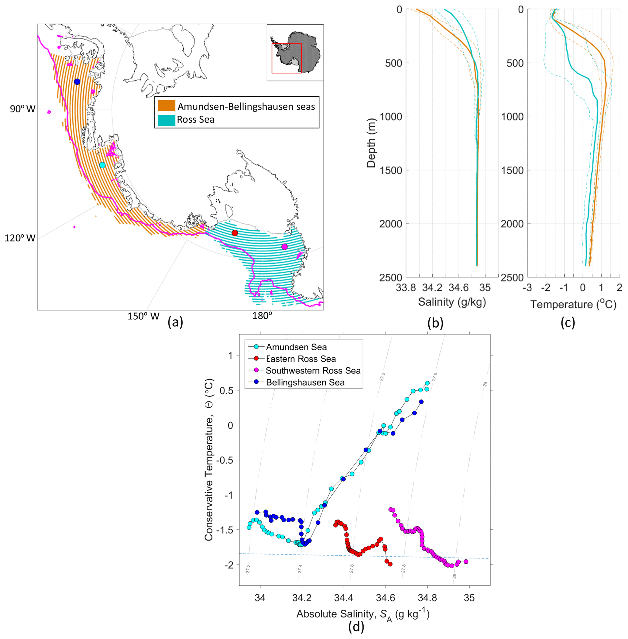
Figure 1(a) The study domain of Amundsen–Bellingshausen seas and Ross Sea with bathymetry above 2500 m. The magenta line indicates the 1000 m IBCSO depth contour. Panels (b) and (c) show geographically averaged decadal (1995–2004) WOA salinity and temperature profiles in the Amundsen–Bellingshausen seas (orange; corresponding to the orange stippled region in a) and the Ross Sea (cyan; corresponding to the cyan stippled region in a). Dashed lines indicate ±1 SD of values at each depth in each region. (d) T–S properties of selected water columns (corresponding to colored circles in a).
In addition to these stark contrasts in regional mean temperature (and salinity), there is also significant spatial variability within each region of the ABRS and across the continental shelf break. For example, Fig. 1 indicates a high standard deviation (SD) in ocean temperature on the continental shelf with water depth shallower than 700 m (0.5 ∘C in the Amundsen–Bellingshausen seas and 1.4 ∘C in the Ross Sea). Much of this variability is attributable to the lateral temperature gradient from the subsurface layer of CDW over the continental slope to the modified (cooled) water masses inshore. In the alongshore direction, vertical profiles of water properties in the Amundsen–Bellingshausen seas are similar, with cold and fresh water overlying relatively warm and salty water. In the Ross Sea, water properties are different on its southwestern and eastern sides, mainly distinguished by their salinity (Fig. 1d).
The sparseness of measurements in the ACSS also aggravates errors associated with gridded observational products. Coastal regions, in particular, are subject to substantial errors. Sun et al. (2019) showed that salinity biases between WOA objective analysis and the World Ocean Database increase toward coastlines. The gridded objective analysis field neglects the dynamical processes governing water mass modifications and circulations induced by complex continental shelf bathymetry (Dunn and Ridgway, 2002; Schmidtko et al., 2013). In sparsely sampled regions, grid-point-based comparisons (e.g., Little and Urban, 2016) are thus of limited utility and may underestimate uncertainty in the reference (observational) product. We suggest that it is often more meaningful to assess GCMs using a regionally averaged approach.
Previous model–data comparisons in the ACSS have employed strategies such as averaging over a priori defined regions (e.g., Barthel et al., 2020). Such methods are ill-equipped to assess model biases resulting from misplaced water masses. An alternative method is objective clustering, which can be used to identify regions of similar hydrographic metrics. For example, Hjelmervik and Hjelmervik (2013) demonstrated the application of a clustering-based approach using Argo profiles to segregate the North Atlantic into groups with similar vertical T and S profiles separated by fronts.
The results of clustering analyses are dependent on the metrics chosen for the analysis. For example, metrics could be chosen as the layer thicknesses of water masses defined by T, S and neutral density. Schmidtko et al. (2014) partitioned water masses in the Southern Ocean into Winter Water (WW), CDW, and Antarctic Shelf Bottom Water (ASBW) using only temperature. However, their metrics of subsurface water temperature maxima and minima are ineffective on the continental shelf, where temperature profiles are often complex and show strong lateral variability in water properties (Fig. 1d). Sallée et al. (2013) proposed a method to use potential vorticity evaluated from density profiles and the local salinity minimum at 30∘ S to distinguish vertical water masses in the Southern Ocean.
In the ACSS, however, the hydrographic structure is complicated not only by the variability of primary water masses but also by transport, mixing, and strong and highly localized interactions between the atmosphere, ocean, sea ice, and ice shelves. Each of these processes is sensitive to vertical and horizontal density gradients and gradients in bathymetry. Metrics that capture the importance of stratification concurrently with dominant water mass characteristics provide the best test of whether a model is representing the principal dynamical processes governing hydrographic variability in the ACSS. Here, we develop new metrics targeted at ACSS hydrography and assess the utility of a clustering-based approach for model–data comparison.
In this paper, we identify hydrographic regimes and their T–S properties using metrics derived from three-dimensional grids of measured and modeled temperature and salinity (Sect. 2.1) using a K-means clustering method (Sect. 2.2). We then apply a clustering algorithm based on data density to exclude outliers (Sect. 2.3) from the resulting “groups”.
2.1 Data and processing
We use decadal-mean, objectively analyzed T and S fields from WOA for 1995–2004, with 0.25∘ resolution in both latitude and longitude. The data sources, quality controls and processing procedures of the WOA are detailed in Locarnini et al. (2019) for temperature and Zweng et al. (2019) for salinity. This study focuses on the domain from the west of Cape Adare (163∘ E) on the western side of the Ross Sea to the southern end of Alexander Island (76∘ W), at depths between 0 and 2500 m. The landward limit of the study domain is the Antarctic coast and the ice shelf edges as identified in Fig. 1a.
We compare the Community Earth System Model version 2 (CESM2; Danabasoglu et al., 2020) to WOA for the same period and domain. The time-mean model salinity and temperature fields over the 1995–2004 period are calculated from the monthly output of the Coupled Model Intercomparison Project Phase 6 (CMIP6) historical simulation (experiment tag r1i1p1f1) (Eyring et al., 2016) at the native ocean model resolution (roughly 1∘ in longitude and 0.5∘ in latitude). CESM2 uses the CICE5 (Hunke et al., 2015) sea ice model; however, dynamic and thermodynamic interactions with land ice are not represented (Danabasoglu et al., 2020). The CMIP6 forcing data are described in Eyring et al. (2016) and can be download from input4MIPs (https://esgf-node.llnl.gov/search/input4MIPs, last access: 15 October 2020).
We used the Gibbs SeaWater (GSW) Oceanographic Toolbox of TEOS–10 (McDougall and Barker, 2011) to calculate seawater properties. The absolute salinity (SA) is given in units of g kg−1, and conservative temperature (Θ) is given in ∘C. All seawater temperatures are referenced to the sea surface.
2.2 Prototype-based clustering technique (K-means)
The K-means clustering analysis used in this study is an unsupervised learning technique that classifies data into meaningful groups based on their similarity. In this study, the similarity is defined by two metrics of the water column: (1) salinity at the temperature minimum and (2) salinity at the temperature maximum. The rationale for these choices is discussed in Sect. 3.1.
The K-means algorithm is initialized by randomly selecting data in N dimensions (here, N=2, for the two specified metrics) for a specified number of groups (K). For each group (ki), the sum of squared distance (SSD) of each data point (ξ) to the group's centroid (ci) is calculated as follows:
where dist is the standard distance between data and centroid in N-dimensional Euclidean data space and mi is the total number of data points in group ki. The algorithm iterates to minimize SSD by adjusting the centroids, recalculating the distances and redistributing data points among the groups. The K-means algorithm will have multiple solutions because it is initialized with randomly selected data. We apply the K-means 1000 times and choose the solution with the lowest SSD for analysis.
The K-means algorithm requires specification of the number of groups (K). We use silhouette scores si(n) (Eq. 2) to assess the appropriate values of K.
In Eq. (2), n represents the number of data points in group ki, a(ξ) is the mean dist from a data point ξ to all other data points within the group ki and b(ξ) is mean dist from ξ to all other data points outside the group ki. Silhouette scores are evaluated for each data point ξ in the group ki and range between −1 and 1. If ξ lies perfectly at the centroid of group ki, then si(n)=1.
A rigid interpretation of the silhouette algorithm would choose the value of K that corresponds to the highest mean value of si(n). However, the optimal K value can vary with different clustering evaluation methods (e.g., the elbow method; Thorndike, 1953) and different domains. The selection of K is thus based not only on the results of silhouette assessment but also on the ability to interpret the groups as representative of different underlying physical processes (see Sect. 3).
2.3 Density-based clustering technique
In subsequent sections, we use a T–S diagram to compare the properties of groups given by the K-means algorithm. We applied a data-density-based clustering technique (DBSCAN) (Ester et al., 1996) to define the “core” of a group and to exclude outliers on the T–S diagram. Note that DBSCAN is only used to highlight the core of a given group and facilitate comparisons of water properties between WOA and CESM2.
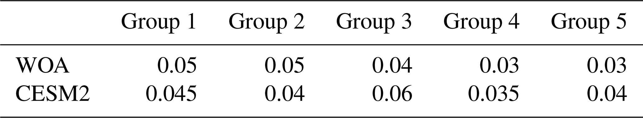
Table 2The coverage (%) of the majority group of DBSCAN in the total non-outlier data.

The T–S core of each hydrographic regime identified by the K-means clustering is determined by the DBSCAN algorithm using two parameters: a radius (ε) and a minimum number of neighboring points (MinPts). The DBSCAN algorithm builds up pools of data by initially choosing a random data point. If the initially chosen data point has less than MinPts within ε, then it is defined as an outlier. If this data point has more than MinPts within ε, then a pool of data is initialized consisting of the initial point and the points within ε (neighbors). The pool grows by continually clustering neighboring points until these points have fewer than MinPts within ε. The algorithm continues until all data points are either clustered into pools of data or labeled as outliers. In the current study, we choose MinPts = 10 and . The value of ε is then selected (Table 1) so that the largest pool of data contains at least 97 % of non-outlier points (Table 2). This pool of data constitutes the core of each group.
3.1 Defining water column metrics
Our goal in this analysis is to utilize key features of local water columns to identify regions with similar hydrographic properties. Such metrics must be able to capture stratification, and the changes in T and S in both along- and cross-shelf directions. For the ACSS, the metrics must include salinity because it is the dominant factor influencing water column stability and reflects critical processes such as brine input during sea ice formation, and freshwater inputs from melting sea ice and ice shelves. By itself, however, salinity poorly represents the vertical composition of water masses since it increases monotonically with water depth over most of the ACSS (Fig. 1); salinity alone is insufficient to identify regimes with sub-surface heat reservoirs that are characteristic of regions with high ice shelf basal melt rates (Rignot et al., 2013; Dinniman et al., 2016; Adusumilli et al., 2020). The metrics we use in this study – salinity at the vertical temperature minimum and salinity at the vertical temperature maximum – are similar to those used by Timmermans et al. (2014) to segregate surface water from Alaskan coastal water in the Central Canada Basin of the Arctic Ocean.
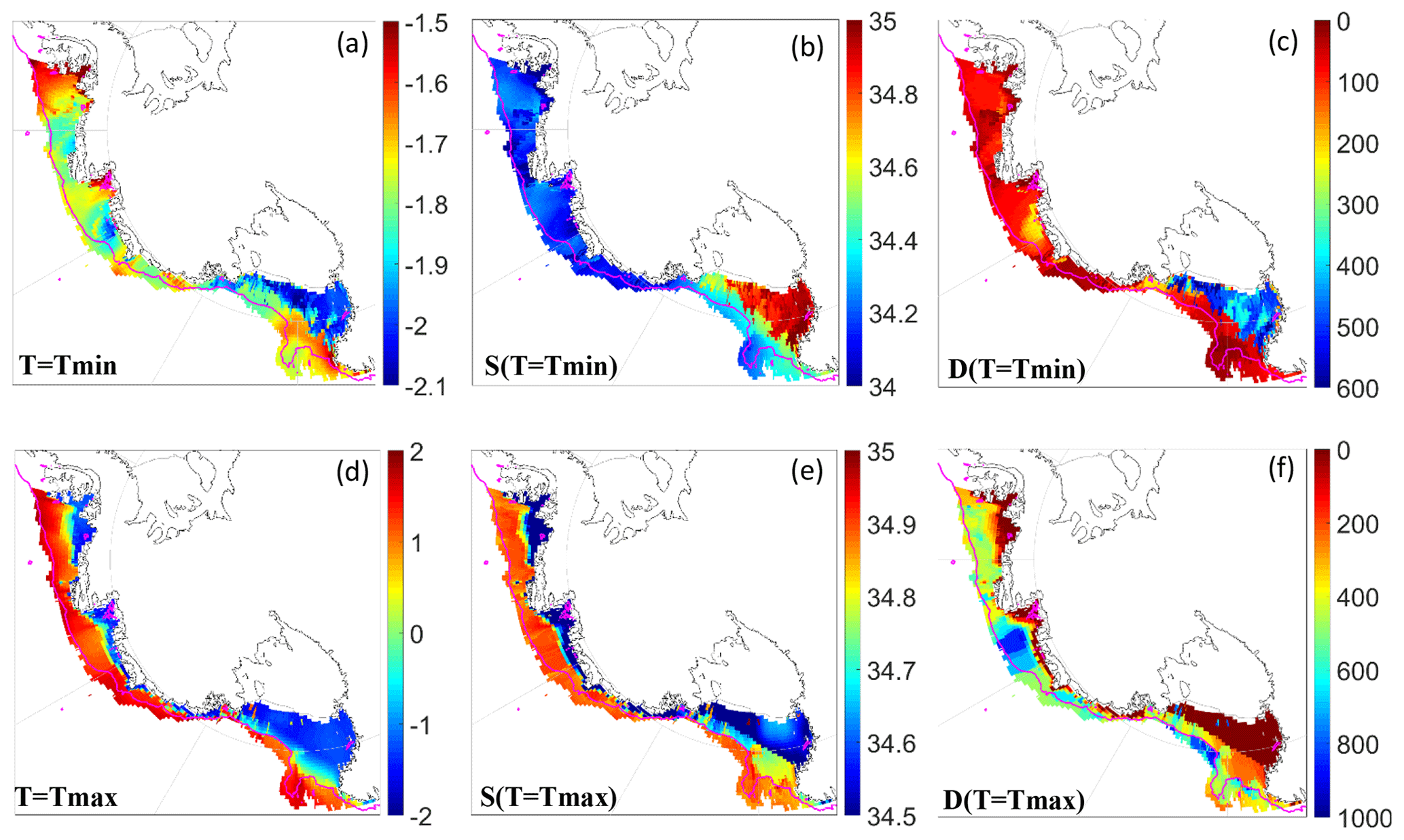
Figure 2Clustering metrics in WOA. Minimum temperature at each grid point (a) and the salinity (b) and water depth at the minimum temperature. Panels (d)–(f) are the same as (a)–(c) but for quantities at the temperature maximum.
Along-shelf variations of water properties are evident in salinity at the vertical temperature minimum (Fig. 2b). In the Amundsen–Bellingshausen seas, the depth of minimum temperature (Fig. 2c) is commonly above 200 m, where salinity is often less than 34.2 g kg−1. In contrast, in the southwestern Ross Sea, the minimum temperature is usually located below 350 m and coincides with much higher salinity (>34.8 g kg−1). The northwestern Ross Sea contains a regime with a local temperature minimum at shallower depths approaching the shelf break, but its salinity (between 34.2 to 34.6 g kg−1) is higher than near-surface water in the Amundsen–Bellingshausen seas.
The salinity at the vertical temperature maximum shows pronounced variations in the cross-shelf direction (Fig. 2d–f). The maximum water temperature (Fig. 2d) is commonly found at depths above 200 m close to the coast and ice shelves (Fig. 2f) and deeper toward the shelf break and over the continental slope where the water depth increases. The salinity at the vertical maximal temperature (Fig. 2e) shows similar variations in the cross-shelf direction, with lower salinity (<34.7 g kg−1) near the coast and ice shelves and higher salinity (>34.8 g kg−1) on the continental shelves and near the shelf break.
3.2 Evaluating the optimum number of groups
We used the mean value of the silhouette score si(n) in Eq. (2) to evaluate an appropriate number of groups (K) for WOA and CESM2, testing (Fig. 3). For WOA, the highest value of si occurs when K=3; for CESM2, K=6 has the highest silhouette score (Fig. 3a and b). The spatial distributions of groups 3, 5 and 6 in the ABRS are shown in Fig. 3c–h.
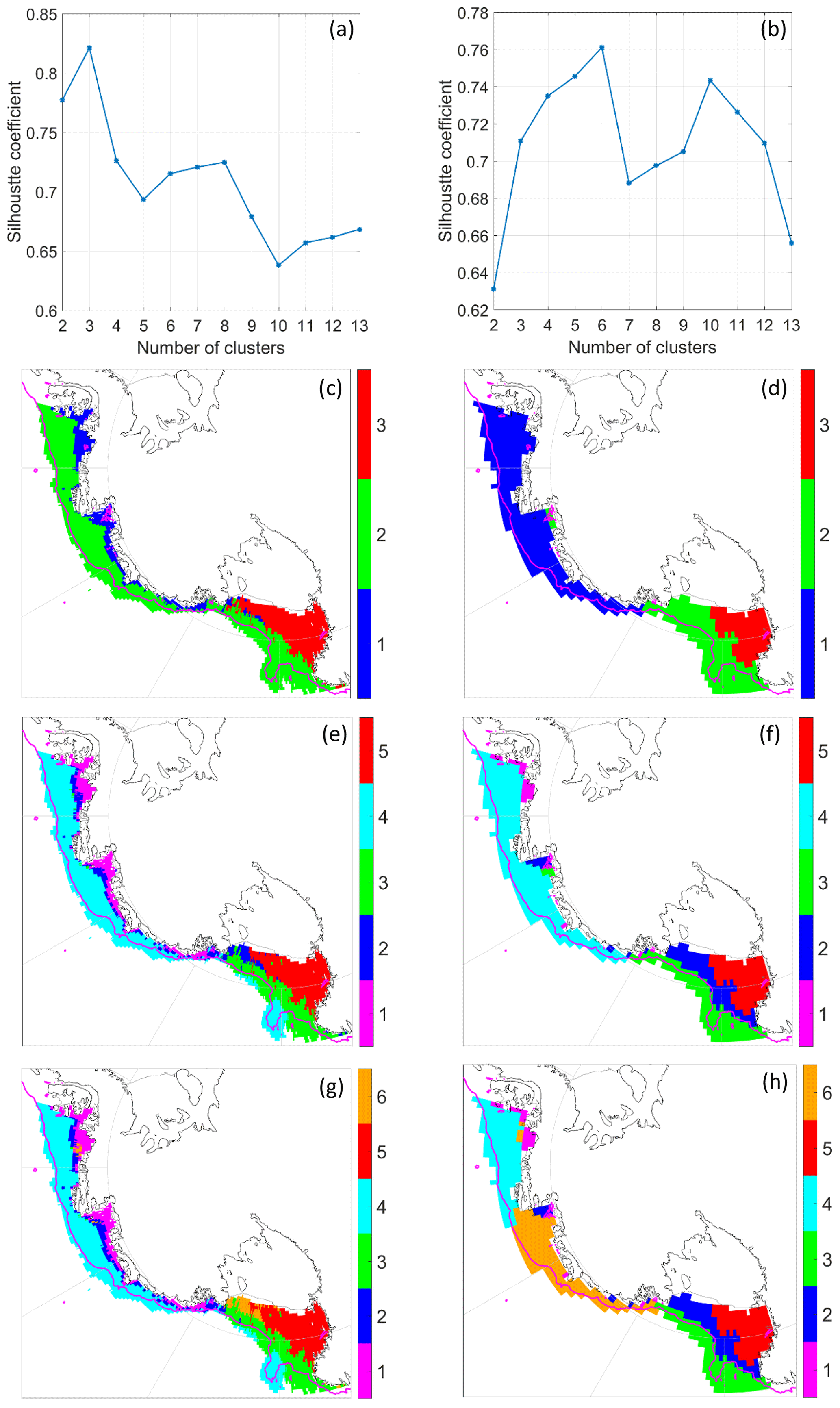
Figure 3K-means clustering evaluation for WOA and CESM. Silhouette analysis is shown in (a) and (b) for WOA and CESM, respectively. The geographic regions corresponding to 3, 5 and 6 groups for WOA, (shown in c, e and g) and for CESM (shown in d, f and h) are shown.
When WOA data are clustered into three groups (Fig. 3c), the K-means algorithm segregates the water close to the Antarctic coast from the water on the shelf and continental slope. The coastal domains are further distinguished into Amundsen–Bellingshausen coastal waters and Ross coastal waters. By increasing the number of groups to five (Fig. 3e), a narrow domain between coastal and shelf waters emerges. In the Ross Sea, waters on the shelf and across the shelf break are segregated into two groups. For K=6 (Fig. 3g), the southeastern coastal domain of the Ross Sea (orange) is further separated from the narrow domain between coastal and shelf waters in the Amundsen–Bellingshausen seas, while the locations of the other groups are generally unchanged.

Figure 4ABRS groups in metric space. Each point corresponds to a grid point, with a color corresponding to its group number, for K=3, 5 and 6, for WOA (shown in a, c and e) and for CESM2 (shown in b, d and f).
Examining the groups with respect to the two metrics used in the K-means clustering (Fig. 4) shows that, when K=3, the groups are separated by the perpendicular lines from the incenter of the triangular T–S distributions (Fig. 4a). As the total number of groups increases, data points are progressively divided into smaller subsets, with an asymmetry that is influenced by their original distribution in our two-metric parameter space, as well as gaps and discontinuities (Fig. 4c and e).
In CESM2, the clusters in the ABRS differ from those for WOA, particularly for K=3 and K=6. For K=3 (Fig. 3d), the entire Amundsen–Bellingshausen seas region is segregated from the Ross Sea, while the southwestern Ross Sea is still recognized as an independent group. For K=6, the Amundsen Sea is segregated from the Bellingshausen Sea. With K=5 (Fig. 3f), CESM2 clustering is qualitatively similar to WOA, with a coastal group emerges in the Amundsen–Bellingshausen seas; however, its areal extent is much smaller than in WOA. In the Ross Sea, the water on the continental shelf is separated from the water on the continental slope, similar to WOA. CESM2 shows a similar range to WOA in metric space (Fig. 4), although with much larger gaps. In particular, CESM2 has substantially fewer data points with intermediate and low salinity (Fig. 4b). Increasing K for clustering analysis of CESM2 output subdivides high-salinity regimes at Tmax based on the distribution of salinity at Tmin (Fig. 4d and f).
Based on the silhouette scores, the optimum clustering for CESM2 is six groups; however, the WOA data have a maximum silhouette score for K=3. Segregating the WOA into five or six groups is reasonable, as the clustering algorithm continually distinguishes finer differences in the coastal regimes (Fig. 3e and g). However, the segregation of CESM2 into six groups (Fig. 3h) is physically unfair since the water properties below the surface layers are nearly indistinguishable between the Amundsen and Bellingshausen seas (Fig. 1d). Figure 4 also indicates that the segregation of Amundsen–Bellingshausen seas regions in CESM2 is a result of discontinuities between groups 1 and 5 (Fig. 4f). We thus choose to use five groups for the rest of the study. Our findings from analyzing the temperature and salinity properties in the following sections further support this decision.
3.3 Physical interpretation of WOA groups
Vertical profiles of temperature and salinity are shown for each WOA group in Fig. 5. The mean vertical structure of each group is clearly different; furthermore, the standard deviations at each depth within groups are much smaller than those of regional mean profiles (Table 3). With these vertical structures as context, we examine T–S properties at all depths from each WOA group in Fig. 6. The DBSCAN algorithm is used to identify the “core” of non-outlier data in each group, shown with dark shading in Fig. 6.
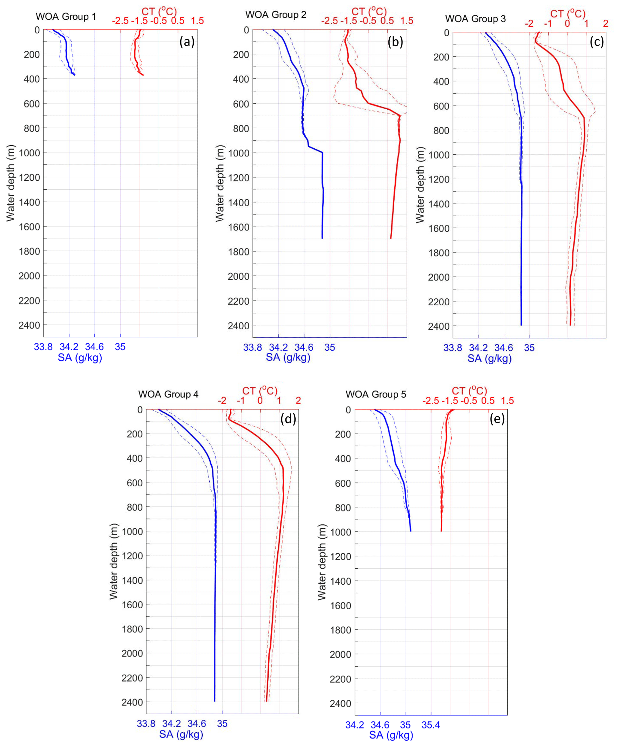
Figure 5Mean (solid lines) WOA salinity (in blue) and temperature (in red) profiles for five groups (from a to e) shown in Fig. 3e; ±1 SD at each depth is shown with dashed lines.
Table 3The salinity and temperature standard deviation of WOA (at depth of 500 m if not specified).
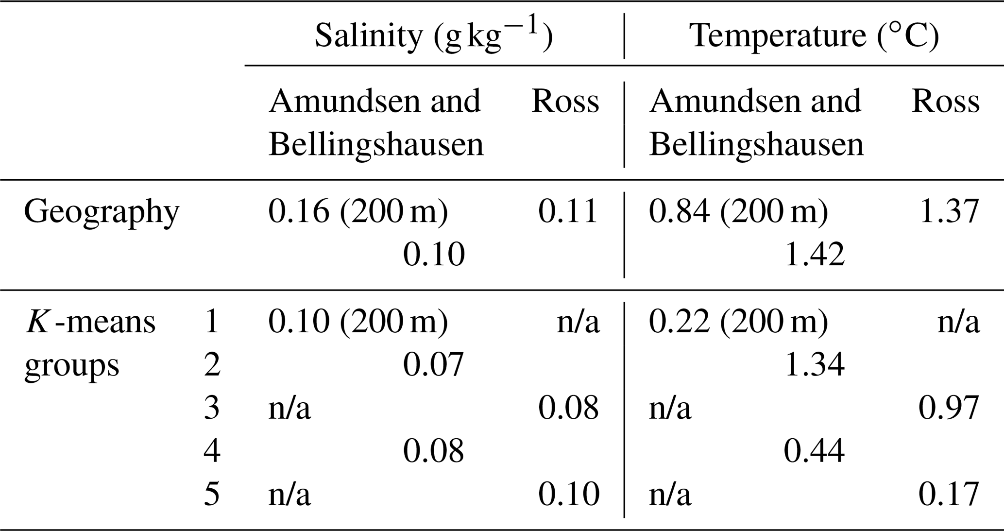
n/a – not applicable.
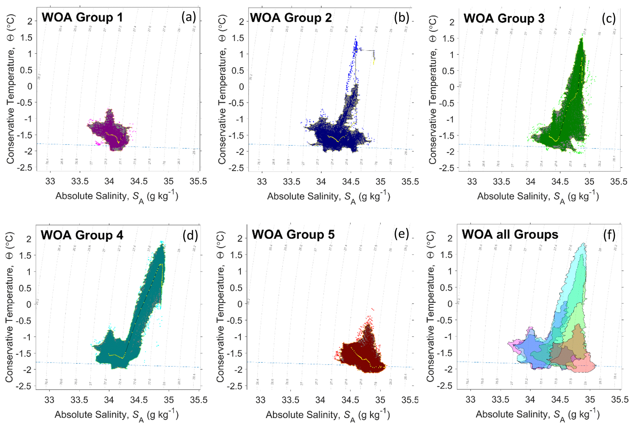
Figure 6T–S properties for the five WOA groups (from a to e) shown in Fig. 3e. The dotted yellow lines show the profile of mean temperature and salinity in each group, and the dark shaded areas are the cores of water property from the density-based clustering results. The cores of all five groups are overlaid on the same plot in (f).
Group 1, which occupies the inshore regions of the Amundsen–Bellingshausen seas (Fig. 3e), is characterized by weak vertical gradients in both T and S over the ∼400 m water column (Fig. 5a). The water in this group has relatively low salinity (33.8 to 34.5 g kg−1), temperature close to the freezing point (generally lower than −1 ∘C) and low density (26.9 and 27.5 kg m−3) (Fig. 6a), which suggests that the water in this regime is strongly influenced by coastal freshwater input (Moffat et al., 2008; Jacobs and Giulivi, 2010; Jourdain et al., 2017).
Group 2, which is spatially located between the coastal waters (groups 1 and 5) and outer continental shelf waters (groups 3 and 4), represents a narrow domain of mixing (Fig. 3e). This regime is characterized by relatively high standard deviations in salinity and temperature at depths between 100 and 700 m, indicating that the location and shape of the thermocline and halocline above the typical depth of the shelf break vary within this group (Fig. 5b). Below 700 m, the range of salinity and temperature are relatively small, due to reduced the limited amount of data at these depths over the relatively narrow continental slope. In the upper ocean, group 2 has a salinity from 33.8 to 34.7 g kg−1, temperature from −2 to −0.5 ∘C and density from 27.1 to 27.8 kg m−3 (Figs. 5b and 6b), lying between the properties of surface waters in groups 1 and 5. In the subsurface, group 2 has a temperature above −0.5 ∘C and salinity above 34.5 g kg−1, which represents modified CDW on the shelf (Carmack, 1977; Orsi and Wiederwohl, 2009; Emery, 2011).
Group 3, which is found on the outer continental shelf and the continental slope of the Ross Sea (Fig. 3e), shows high standard deviations in temperature above 700 m (Fig. 5c), similar to group 2. However, the water in this regime is generally denser than group 2. The surface water in group 3 is fresher than that of group 5 (Figs. 5c and 6c, f), which may result from sea ice melt and/or lateral mixing with fresher shelf water originating in the Amundsen–Bellingshausen seas (Assmann et al., 2005; Porter et al., 2019). The subsurface water (between 100 and 600 m) of group 3 (Figs. 5c and 6c) does not have a clear vertical water mass transition, and denser water exhibits a wide temperature range (−1.5 to +1.5 ∘C) with relatively high salinity (34.6 to 35 g kg−1), suggestive of mixing between High-Salinity Shelf Water (HSSW) and CDW.
Group 4, on the continental shelf of the Amundsen–Bellingshausen seas and along most of the continental slope of the ABRS (Fig. 3e), exhibits properties consistent with off-shelf Southern Ocean water, as noted by Schmidtko et al. (2014). It has a well-defined vertical temperature structure with limited spatial variability (Fig. 5d). In this region, Winter Water (WW) with salinity of 33.8 to 34.5 g kg−1, temperature of −2 to −0.5 ∘C and density of 27 to 27.5 g m−3 overlies CDW (salinity 34.6 to 36.8 g kg−1, temperature 0 to +2 ∘C and density 27.8 to 27.9 g m−3), with a mean profile showing a clear transition between them (Fig. 6d).
Group 5, in the southwestern Ross Sea with some extensions to the southeast (Fig. 3e), has higher salinity than other groups (Fig. 6). The almost uniform vertical temperature profile (Fig. 5e) is identified as HSSW. It is characterized by salinity 34.3 to 35.1 g kg−1, temperature close to the freezing point, and density of 27.5 to 28.1 kg m−3 (Fig. 6e), resulting from brine rejection in the polynyas along the coast and Ross Ice Shelf front (Foster and Carmack, 1976). The surface portion of the waters in group 5 with salinity lower than 34.62 g kg−1 is often defined as Low-Salinity Shelf Water (LSSW) in the Ross Sea shelf, but we generally refer to group 5 as HSSW because its volume is much higher than the LSSW (Orsi and Wiederwohl, 2009).
Overall, groups 1 and 5 (Fig. 6a and e) show relatively homogeneous salinity and temperature, while group 4 has a pronounced thermocline and halocline at shallow depth. These three groups (1, 4 and 5) represent the three “primary” ABRS hydrographic regimes. In contrast to these primary regimes, groups 2 and 3 have more complex vertical structures, more spatial variability in thermocline at depths above about 600 m (roughly the shelf break) and can be considered “mixed” regimes.
3.4 Assessing groups in CESM2
To identify hydrographic regimes in CESM2, we conduct the same analyses as described for WOA in the previous section, focusing on results for K=5 (Fig. 3f). The T–S properties of each group in CESM2 are shown in Fig. 7. CESM2 results are similar to WOA's in that three primary regimes are present (group 1, coastal fresh-water-enriched; group 4, off-shelf; and group 5, HSSW), but they show differences in their spatial extent (Fig. 3e vs. f), volume (Table 4) and T–S properties (Fig. 8).
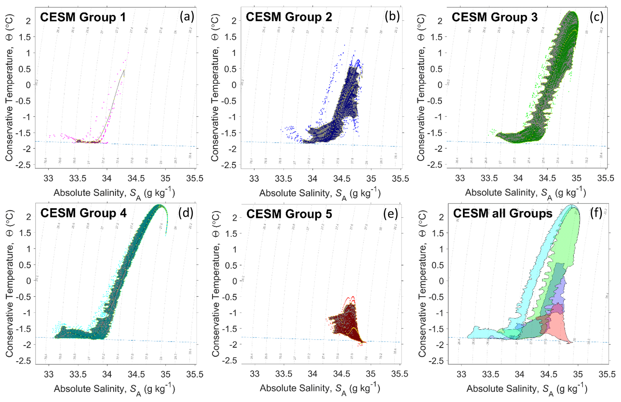
Figure 7As in Fig. 6 but for the five groups identified in CESM2 (from a to e) shown in Fig. 3f.
Table 4The percentage of clustered water in the total ocean volume in the ABRS.

As in WOA, HSSW (group 5) of CESM2 is localized in the southwestern Ross Sea, but its eastward extension into the southeastern Ross Sea is missing in CESM2 (Fig. 3e and f), resulting in a reduced HSSW volume (Table 4). The coastal fresh-water-enriched regime (group 1) is mostly absent in CESM2 and is replaced by the off-shelf regime in the Amundsen Sea.

Figure 8The core of water properties in WOA (red) and CESM2 (blue). Note that groups 2 and 3 have been combined for CESM2.
Mismatches between CESM2 and WOA are also evident in the T–S properties of these primary regimes. In general, HSSW in CESM2 has a fresh and warm bias relative to WOA (Fig. 8d). Combined with its reduced volume relative to WOA, this bias in CESM2 HSSW properties suggests that weak modeled katabatic winds in the southwestern Ross Sea may limit sea ice production and export. Group 4 (the off-shelf regime) exhibits a fresh bias in WW in the upper water column, but the densest off-shelf water in group 4, i.e., CDW, is saltier and warmer (Fig. 8c). Sea ice concentrations are biased low in CESM due to positive zonal wind stress biases in the Southern Ocean (Singh et al., 2020). This wind stress bias may, in turn, lead to an overestimate of the upwelling of warm and salty CDW onto the ACSS. The limited extent of the coastal fresh-water-enriched regime (group 1) in CESM2 may result from the absence of basal melt from ice shelves.
The mixed regimes shift geographic location in CESM2. The narrow mixing zone (group 2) between coastal fresh-water-enriched and off-shelf regimes in the Amundsen–Bellingshausen seas is not evident in CESM2 (Fig. 3e and f); the CESM2 is likely too coarse to resolve these mixing fronts. In the Ross Sea, groups are separated into on-shelf (group 2) and off-shelf (group 3) approximately along the 1000 m isobath (Fig. 3f). CESM2 fails to show the path of export of Ross on-shelf water (group 2, Fig. 3f) along the northwestern continental slope (Orsi et al., 1999) as it is seen in the WOA (group 3, Fig. 3e). The core of on-shelf water (group 2) also has less overlap with HSSW (group 5) in the T–S diagram in CESM2 (Fig. 7f) compared to WOA (Fig. 6f). It is possible that these differences result from the overflow parameterization in CESM2 (Briegleb et al., 2010). In this parameterization, locations of the on-shore source water at its formation regions and off-shore entrainment, which mixes with the source water to produce the final water mass, are defined, and overflow water is routed to fixed locations. While this parameterization allows transport of HSSW to the Southern Ocean, it is entirely artificial and does not represent on-shelf mixing processes.
3.5 Assessing clustering over the ACSS
As the K-means algorithm is based on purely statistical criteria (centroid and minimized SSD in Eq. 1) applied to specific metrics, it is valuable to assess whether clustering results are sensitive to different study domains. As a test case, we apply the same algorithm to WOA over the entire circumpolar ACSS where total water depth is less than 2500 m. The metrics used as input for the K-means analysis, as well as the total number of groups (K=5), are unchanged. The use of the uniformly gridded WOA product, rather than observational data, avoids the possibility that the comparison is biased by regional variations in data density.
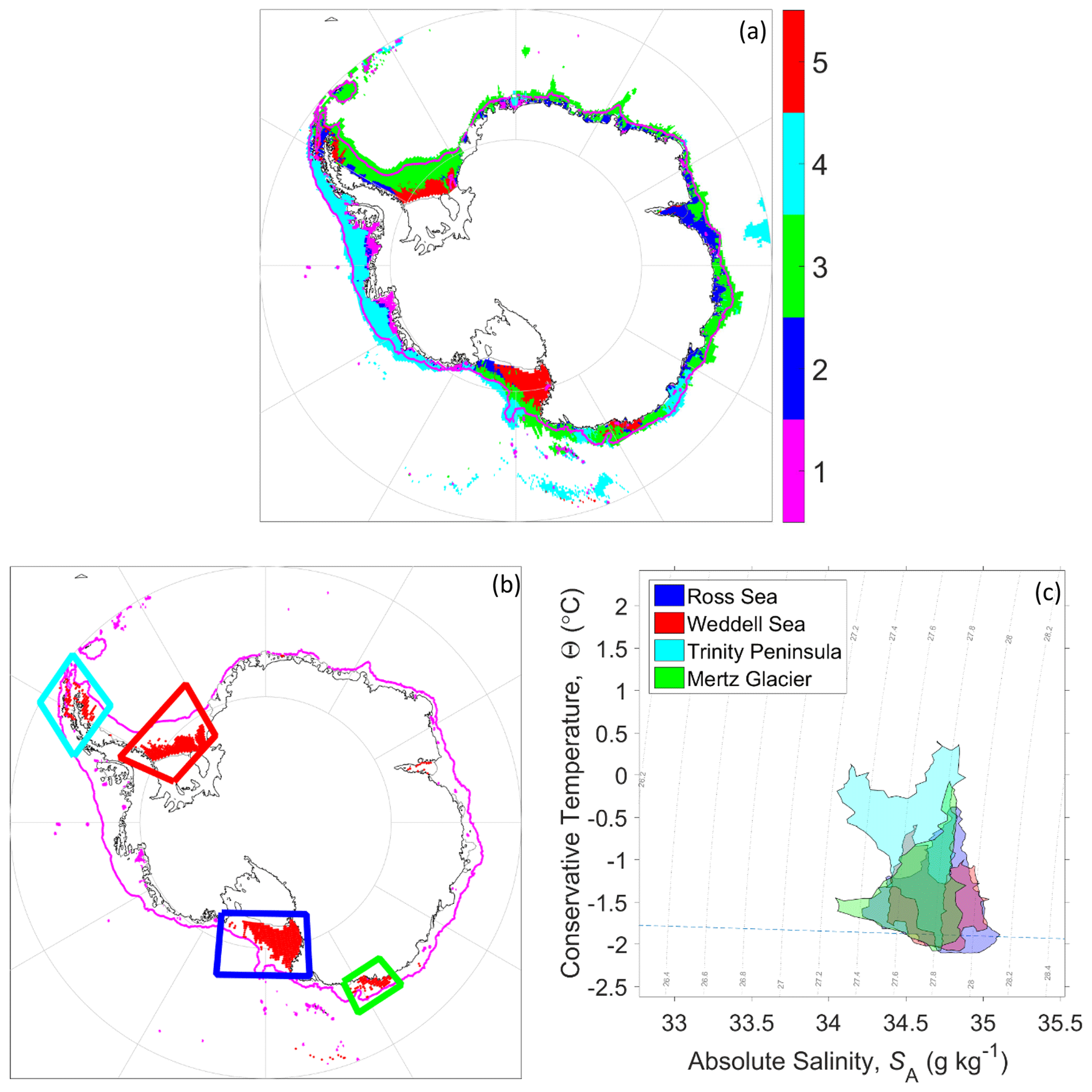
Figure 9(a) WOA-based groups on the entire ACSS (same color code as Fig. 3e). (b) Four places are identified as HSSW regimes with the following color coding: blue is the southwestern Ross Sea, red is the Weddell Sea near the Filchner–Ronne Ice Shelf and the George V Coast, cyan is the Bransfield Strait and south of Trinity Peninsula, and green is the Mertz Glacier tongue. (c) T–S properties of group 5 (HSSW) regions, with their geographic location and color code matched in (b).
The location of five clustered water groups over the entire ACSS is shown in Fig. 9a. Within the ABRS domain, the geographic locations of all groups are almost unchanged, indicating the clustering results in the ABRS are insensitive to substantial enlargement of the domain. The region identified as group 5 in the southwestern Ross Sea, which is associated with HSSW formation, remains. Outside the ABRS, the clustering approach identifies water of similar properties to group 5 in the Weddell Sea near the Filchner–Ronne Ice Shelf, the George V Coast near the Mertz Glacier tongue, and Bransfield Strait and south of Trinity Peninsula (regions marked on Fig. 9b). The southern Weddell Sea experiences similar conditions to the southwestern Ross Sea, with HSSW formation in winter due to brine rejection from sea ice formation enhanced by katabatic winds and tides driving a narrow but persistent along-ice-front polynya (Nicholls et al., 2009). Along the George V Coast, HSSW is also generated by similar processes acting near the Mertz Glacier ice tongue (Bindoff et al., 2000; Post et al., 2011).
The waters in the subsurface of Bransfield Strait and south of the Trinity Peninsula are also grouped with the HSSW regions, although their surface water is warmer and fresher than that of other HSSW regions around Antarctica. Cook et al. (2016) showed that the regional water properties around the tip of the Antarctica Peninsula, based on the World Ocean Database, are very similar to HSSW. Gordon et al. (2000) also noted that the water properties in the center of Bransfield Strait are similar to HSSW in the Weddell Sea; they inferred that these waters are formed in western Weddell Sea coastal polynyas and flow into Bransfield Strait.
We have shown that the ABRS can be clustered into different regions based on salinity at the vertical water temperature minimum and maximum. This technique can help identify regions in model and observational datasets in which water properties are controlled by similar physical processes. This is in contrast to traditional grid-point-based comparisons, which do not adequately account for misplaced water masses.
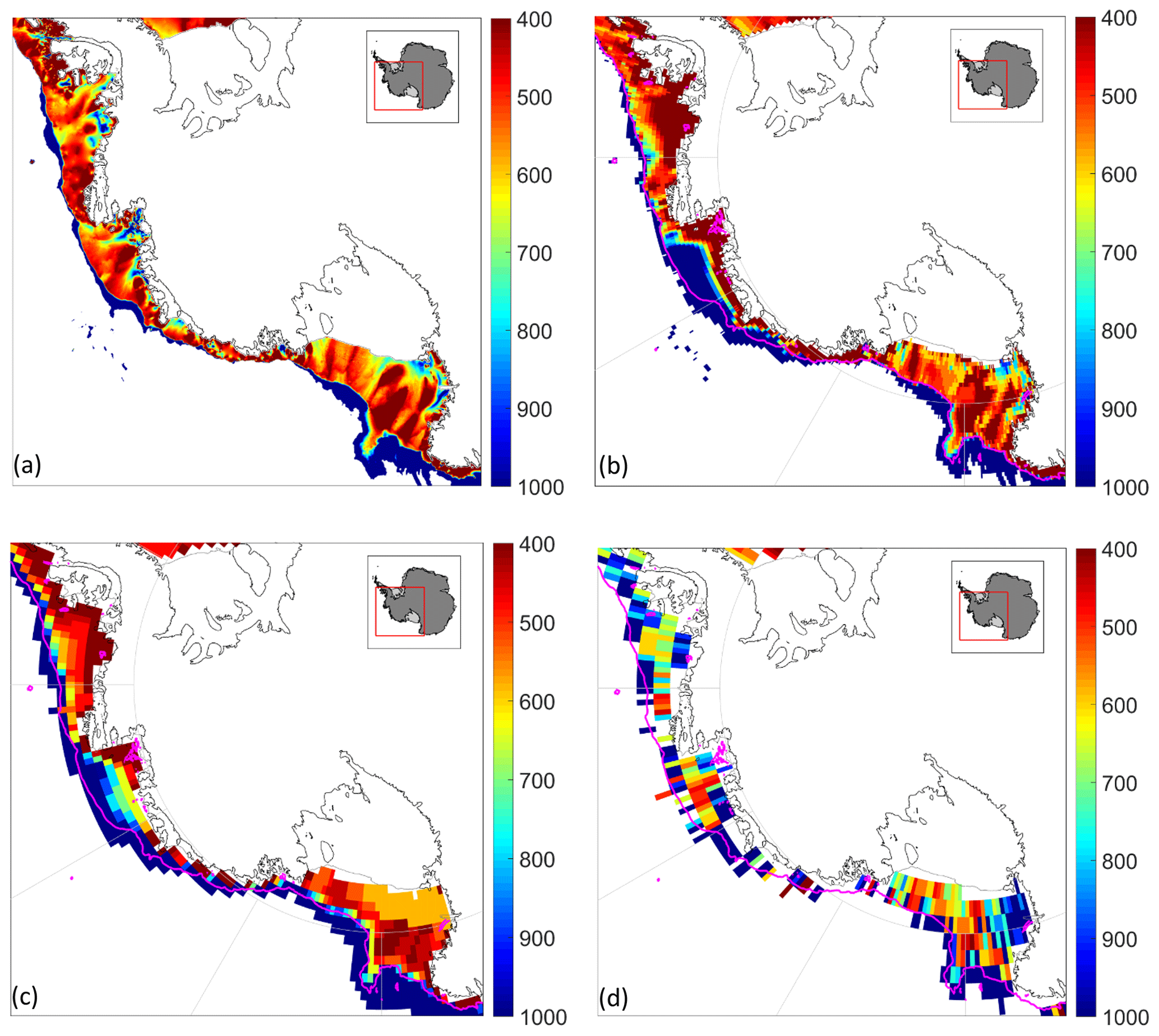
Figure 10Bathymetry between 400 and 1000 m of (a) IBCSO (500 m horizontal resolution), (b) WOA (0.25∘ horizontal resolution), (c) CESM2 (1×0.5∘ long/lat resolution) and (d) the WOD bin-averaged into 1∘ horizontal resolution with all types of instrument with temperature measurements. The magenta line indicates the 1000 m IBCSO depth contour.
In this study, WOA has been employed to assess CESM2 results. However, the hydrographic regimes identified in WOA may be misleading if they result from interpolation and extrapolation artifacts associated with non-uniform sampling of data in time and space or if the water column structures are not adequately represented in WOA. One source of uncertainty in WOA arises from differences between true and gridded bathymetry, complicating interpolation and extrapolation of sparely sampled data into deeper portions of the water column. In Fig. 10, we compare the depths of the deepest available data in WOA and CESM2 with water depths in the International Bathymetric Chart of the Southern Ocean (IBCSO, Arndt, et al., 2013). WOA has a clear misrepresentation of the Amundsen–Bellingshausen seas continental shelf bathymetry (Fig. 10b). First, the 1000 m isobath is shifted substantially landward in the Amundsen Sea. Second, deep across-shelf troughs (e.g., in Fig. 10a) are not represented in the inner shelf of WOA, which possibly affects the value of salinity at the temperature maximum because the CDW is missing in these regions of the Amundsen–Bellingshausen seas.
It is, therefore, unclear whether groups 1 and 2 are separated from the shelf and continental slope waters of group 4 in WOA (Fig. 3e) due to their upper-ocean freshwater enrichment relative to other groups or if the groups are influenced by under-sampling of hydrography in deep troughs of the Amundsen–Bellingshausen seas. We note that the bathymetry of CESM2 has similar issues to WOA in the Amundsen–Bellingshausen seas (Fig. 10c). Neither WOA nor CESM2 represents the water in deep troughs below about 300 m in these regions, and thus the differences in the groups between WOA and CESM2, i.e., the missing group 1 in the Amundsen coast and narrow group 2 in the Bellingshausen Sea, are unlikely to be due to the bathymetric misrepresentation (Fig. 3e and f). We suggest, instead, that the mismatch of water properties is likely to be induced by the misrepresentation of freshwater input or unresolved coastal currents in CESM2 (Tseng et al., 2016; Sun et al., 2017).
We have highlighted a key advantage to assessing models with clustering-based approaches compared to traditional grid-point-based methods: the ability to identify geographic displacements of hydrographic regimes and to distinguish these displacements from biases in water mass T–S properties. In addition, this approach minimizes potential biases introduced during gridding or re-gridding of data and models to a common grid for comparison studies. For example, it is possible to circumvent interpolation-related issues associated with using scattered and/or sparse data. Such datasets might include individual observations or model output on a native grid. For example, the deepest observational temperature measurements in the World Ocean Database 2018 (WOD), even at a 1∘ resolution, show that observations are available in coastal Amundsen–Bellingshausen seas troughs that are not present in IBCSO (compare Fig. 10d with a); see also Padman et al. (2010). More broadly, the WOD-based salinity and temperature climatology of Sun et al. (2019) reveals that its use can avoid biases created by spatial interpolation of shelf water with off-shelf water.
The success of this technique at identifying locations and properties of HSSW regimes at other locations on the Antarctic continental shelf suggests that it might be used to evaluate other global and/or regional models on a circum-Antarctic basis. Other metrics might be employed depending on specific research goals. For example, the pycnocline depth or the mean or maximum temperature below a fixed depth may be better metrics of subsurface water masses. It will also be interesting to track water masses and their pathways with metrics based on their characteristic properties. However, we note that comparisons of the locations of groups could become complex if the approach is applied to multiple models with substantial biases between their representations of specific water masses.
We have demonstrated the utility and sensitivity of a clustering-based approach for assessing hydrographic regimes and their water properties on the Antarctic continental shelf, using the World Ocean Atlas objective analysis product (WOA) and numerical model output from the Community Earth System Model version2 (CESM2). We segregated the waters in the ABRS into five physically interpretable groups using the salinity at the minimum and maximum temperature of each water column in the domain. The method identifies High-Salinity Shelf Water (HSSW), coastal fresh-water-enriched, and off-shelf hydrographic regimes in observations and the model. Water on the continental shelf and upper continental slope in the ABRS generally shows a warm bias in CESM2 compared to WOA. The near-surface ocean in CESM2 is generally fresher than in WOA but lacks a well-defined fresh-water-enriched coastal current. In the subsurface, CESM2 is saltier in regions of Circumpolar Deep Water but fresher than WOA in HSSW formation regions. Our comparison suggests that mean-state biases of CESM2 in the ACSS result from both local and remote processes, including overestimated zonal winds in the Southern Ocean, unrepresented thermodynamic interactions with ice shelves, and the inadequate representation of overflows in the Ross Sea. A more specific investigation of coastal processes, Southern Ocean dynamics and atmospheric forcing will help further identify the cause of these biases.
The clustered hydrographic regimes in the ABRS are largely unchanged when our method is applied to the entire circum-Antarctic Continental Shelf sea area. HSSW-characterized regimes emerge in WOA in the southern Weddell Sea, near Mertz Glacier tongue and in Bransfield Strait. Future work will focus on applying this approach to a wider range of models (e.g., CMIP6 output and circum-Antarctic simulations) and establishing techniques to work with scattered observational data. Finally, we note that the clustering results for the ACSS based on the WOA decadal data (1995–2004) are consistent with the results based on the most modern WOA decadal data (2005–2017). However, clustering, applied to a variety of metrics, provides the potential to identify more subtle temporal changes in hydrographic fields such as changes in regime extent in the absence of significant changes in water mass characteristics in the ACSS.
The data used in this study are publicly available via the links below: World Ocean Atlas 2018 at https://www.nodc.noaa.gov/OC5/woa18/woa18data.html (NOAA, 2021a); World Ocean Database 2018 at https://www.nodc.noaa.gov/OC5/WOD/pr_wod.html (NOAA, 2021b); and CESM2 data at https://esgf-node.llnl.gov/search/cmip6/ (WCRP, 2021).
QS performed the analyses and wrote the article. CML, AMB, and LP conceived the research idea, directed the project, and supported the article revision.
The authors declare that they have no conflict of interest.
The authors thank the NCAR climate modeling groups for producing and distributing the CESM2 output.
This research has been supported by the NSF (grant no. 1744789), NASA (grant no. NNX17AG63G), and the DOE (HiLAT-RASM project).
This paper was edited by Trevor McDougall and reviewed by two anonymous referees.
Adusumilli, S., Fricker, H. A., Medley, B., Padman, L., and Siegfried, M. R.: Interannual variations in meltwater input to the Southern Ocean from Antarctic ice shelves, Nat. Geosci., 13, 616–620, 2020.
Agosta, C., Fettweis, X., and Datta, R.: Evaluation of the CMIP5 models in the aim of regional modelling of the Antarctic surface mass balance, The Cryosphere, 9, 2311–2321, https://doi.org/10.5194/tc-9-2311-2015, 2015.
Arndt, J. E., Schenke, H. W., Jakobsson, M., Nitsche, F. O., Buys, G., Goleby, B., Rebesco, M., Bohoyo, F., Hong, J., Black, J., Greku, R., Udintsev, G., Barrios, F., Reynoso-Peralta, W., Taisei, M., and Wigley, R.: The International Bathymetric Chart of the Southern Ocean (IBCSO) Version 1.0 – A new bathymetric compilation covering circum-Antarctic waters, Geophys. Res. Lett., 40, 3111–3117, 2013.
Assmann, K. M., Hellmer, H. H., and Jacobs, S. S.: Amundsen Sea ice production and transport, J. Geophys. Res.-Oceans, 110, C12013, https://doi.org/10.1029/2004JC002797, 2005.
Barthel, A., Agosta, C., Little, C. M., Hattermann, T., Jourdain, N. C., Goelzer, H., Nowicki, S., Seroussi, H., Straneo, F., and Bracegirdle, T. J.: CMIP5 model selection for ISMIP6 ice sheet model forcing: Greenland and Antarctica, The Cryosphere, 14, 855–879, https://doi.org/10.5194/tc-14-855-2020, 2020.
Bindoff, N. L., Rosenberg, M. A., and Warner, M. J.: On the circulation and water masses over the Antarctic continental slope and rise between 80 and 150 E, Deep-Sea Res. Pt. II, 47, 2299–2326, 2000.
Briegleb, B. P., Danabasoglu, G., and Large, W. G.: An Overflow parameterization for the ocean component of the Community Climate System Model, University Corporation for Atmospheric Research, No. NCAR/TN-481+STR, https://doi.org/10.5065/D69K4863, 2010.
Bromwich, D. H., Nicolas, J. P., Monaghan, A. J., Lazzara, M. A., Keller, L. M., Weidner, G. A., and Wilson, A. B.: Central West Antarctica among the most rapidly warming regions on Earth, Nat. Geosci., 6, 139–145, https://doi.org/10.1038/ngeo1671, 2013.
Carmack, E. C.: Water characteristics of the Southern Ocean south of the Polar Front, in: Voyage of Discovery: George Deacon 70th Anniversary, edited by: Angel, M., Pergamon, Oxford, 1977.
Castagno, P., Capozzi, V., DiTullio, G. R., Falco, P., Fusco, G., Rintoul, S. R., Spezie, G., and Budillon, G.: Rebound of shelf water salinity in the Ross Sea, Nat. Commun., 10, 1–6, 2019.
Cook, A. J., Holland, P. R., Meredith, M. P., Murray, T., Luckman, A., and Vaughan, D. G.: Ocean forcing of glacier retreat in the western Antarctic Peninsula, Science, 353, 283–286, 2016.
Danabasoglu, G., Lamarque, J. F., Bachmeister, J., Bailey, D. A., DuVivier, A. K., Edwards, J., Emmons, L. K., Fasullo, J., Garcia, R., Gettelman, A., Hannay, C., Holland, M. M., Large, W. G., Lawrence, D. M., Lenaerts, J. T. M., Lindsay, K., Lipscomb, W. H., Mills, M. J., Neale, R., Oleson, K. W., Otto-Bliesner, B., Phillips, A. S., Sacks, W., Tilmes, S., van Kampenhout, L., Vertenstein, M., Bertini, A., Dennis, J., Deser, C., Fischer, C., Fox-Kember, B., Kay, J. E., Kinnison, D., Kushner, P. J., Long, M. C., Mickelson, S., Moore, J. K., Nienhouse, E., Polvani, L., Rasch, P. J., and Strand, W. G.: The Community Earth System Model version 2 (CESM2), J. Adv. Model. Earth Sy., 12, e2019MS001916, https://doi.org/10.1029/2019MS001916, 2020.
DeConto, R. M. and Pollard, D.: Contribution of Antarctica to past and future sea-level rise, Nature, 531, 591–597, 2016.
Dinniman, M. S., Asay-Davis, X. S., Galton-Fenzi, B. K., Holland, P. R., Jenkins, A., and Timmermann, R.: Modeling ice shelf/ocean interaction in Antarctica: A review, Oceanography, 29, 144–153, 2016.
Dunn, J. R. and Ridgway, K. R.: Mapping ocean properties in regions of complex topography, Deep-Sea Res. Pt. I, 49, 591–604, 2002.
Emery, W. J.: Water types and water masses, Encyclopedia of Ocean Sciences, 6, 3179–3187, 2011.
Ester, M., Kriegel, H. P., Sander, J., and Xu, X.: A density-based algorithm for discovering clusters in large spatial databases with noise, KDD, 96, 226–231, 1996.
Eyring, V., Bony, S., Meehl, G. A., Senior, C. A., Stevens, B., Stouffer, R. J., and Taylor, K. E.: Overview of the Coupled Model Intercomparison Project Phase 6 (CMIP6) experimental design and organization, Geosci. Model Dev., 9, 1937–1958, https://doi.org/10.5194/gmd-9-1937-2016, 2016.
Foster, T. D. and Carmack, E. C.: Frontal zone mixing and Antarctic Bottom Water formation in the southern Weddell Sea, Deep Sea Research and Oceanographic Abstracts, 23, 301–317, 1976.
Gardner, A. S., Moholdt, G., Scambos, T., Fahnstock, M., Ligtenberg, S., van den Broeke, M., and Nilsson, J.: Increased West Antarctic and unchanged East Antarctic ice discharge over the last 7 years, The Cryosphere, 12, 521–547, https://doi.org/10.5194/tc-12-521-2018, 2018.
Gordon, A. L., Mensch, M., Zhaoqian, D., Smethie Jr., W. M., and De Bettencourt, J.: Deep and bottom water of the Bransfield Strait eastern and central basins, J. Geophys. Res.-Oceans, 105, 11337–11346, 2000.
Hjelmervik, K. T. and Hjelmervik, K.: Improved estimation of oceanographic climatology using empirical orthogonal functions and clustering, in: 2013 MTS/IEEE OCEANS-Bergen, 1–5, IEEE, Bergen, Norway, https://doi.org/10.1109/OCEANS-Bergen.2013.6607987, 2013.
Hobbs, W. R., Massom, R., Stammerjohn, S., Reid, P., Williams, G., and Meier, W.: A review of recent changes in Southern Ocean sea ice, their drivers and forcings, Global Planet. Change, 143, 228–250, 2016.
Holland, M. M., Landrum, L., Raphael, M., and Stammerjohn, S.: Springtime winds drive Ross Sea ice variability and change in the following autumn, Nat. Commun., 8, 1–8, 2017.
Hosking, J. S., Orr, A., Bracegirdle, T. J., and Turner, J.: Future circulation changes off West Antarctica: Sensitivity of the Amundsen Sea Low to projected anthropogenic forcing, Geophys. Res. Lett., 43, 367–376, 2016.
Hunke, E. C., Lipscomb, W. H., Turner, A. K., Jeffery, N., and Elliott, S.: CICE: The Los Alamos Sea Ice Model, Documentation and Software User's Manual, Version 5.1, T-3 Fluid Dynamics Group, Los Alamos National Laboratory, Tech. Rep. LA-CC-06-012, 2015.
Jacobs, S. S. and Giulivi, C. F.: Large multidecadal salinity trends near the Pacific–Antarctic continental margin, J. Climate, 23, 4508–4524, 2010.
Jourdain, N. C., Mathiot, P., Merino, N., Durand, G., Le Sommer, J., Spence, P., Dutrieux, P., and Madec, G.: Ocean circulation and sea-ice thinning induced by melting ice shelves in the Amundsen Sea, J. Geophys. Res.-Oceans, 122, 2550–2573, 2017.
Little, C. M. and Urban, N. M.: CMIP5 temperature biases and 21st century warming around the Antarctic coast, Ann. Glaciol., 57, 69–78, 2016.
Locarnini, R. A., Mishonov, A. V., Baranova, O. K., Boyer, T. P., Zweng, M. M., Garcia, H. E., Reagan, J. R., Seidov, D., Weathers, K. W., Paver, C. R., and Smolyar, I. V.: World Ocean Atlas 2018, Volume 1: Temperature, in: NOAA Atlas NESDIS 81, edited by: Mishonov, A., available at: https://archimer.ifremer.fr/doc/00651/76338/ (last access: 16 January 2021), 2019.
McDougall, T. J. and Barker, P. M.: Getting started with TEOS-10 and the Gibbs Seawater (GSW) oceanographic toolbox, SCOR/IAPSO WG, 127, 1–28, ISBN: 978-0-6465-5621-5, 2011.
Moffat, C., Beardsley, R. C., Owens, B., and Van Lipzig, N.: A first description of the Antarctic Peninsula Coastal Current, Deep-Sea Res. Pt. II, 55, 277–293, 2008.
Nicholls, K. W., Østerhus, S., Makinson, K., Gammelsrød, T., and Fahrbach, E.: Ice-ocean processes over the continental shelf of the southern Weddell Sea Antarctica: A review, Rev. Geophys., 47, RG3003, https://doi.org/10.1029/2007RG000250, 2009.
NOAA: World Ocean Atlas 2018, available at: https://www.nodc.noaa.gov/OC5/woa18/woa18data.html, last access: 16 January 2021a.
NOAA: World Ocean Database 2018, available at: https://www.nodc.noaa.gov/OC5/WOD/pr_wod.html, last access: 16 January 2021b.
Orsi, A. H. and Wiederwohl, C. L.: A recount of Ross Sea waters, Deep-Sea Res. Pt. II, 56, 778–795, 2009.
Orsi, A. H., Johnson, G. C., and Bullister, J. L.: Circulation, mixing, and production of Antarctic Bottom Water, Prog. Oceanogr., 43, 55–109, 1999.
Padman, L., Costa, D. P., Bolmer, S. T., Goebel, M. E., Huckstadt, L. A., Jenkins, A., McDonald, B. I., and Shoosmith, D. R.: Seals map bathymetry of the Antarctic continental shelf, Geophys. Res. Lett., 37, L21601, https://doi.org/10.1029/2010GL044921, 2010.
Paolo, F. S., Fricker, H. A., and Padman, L.: Volume loss from Antarctic ice shelves is accelerating, Science, 348, 327–331, 2015.
Parkinsona, C. L.: A 40-y record reveals gradual Antarctic sea ice increases followed by decreases at rates far exceeding the rates seen in the Arctic, P. Natl. Acad. Sci. USA, 116, 14414–14423, 2019.
Porter, F. D., Springer, S. R., Padman, Laurie, Fricker, Helen A., Tinto, K. J., Riser, S. C., Bell, R. E., the ROSETTA-Ice Team: volution of the Seasonal Surface Mixed Layerof the Ross Sea, Antarctica, ObservedWith Autonomous Profiling Floats, J. Geophys. Res.-Oceans, 124, 4934–4953, 2019.
Post, A. L., Beaman, R. J., O'Brien, P. E., Eléaume, M., and Riddle, M. J.: Community structure and benthic habitats across the George V Shelf, East Antarctica: trends through space and time, Deep-Sea Res. Pt. II, 58, 105–118, 2011.
Rickard, G. and Behrens, E.: CMIP5 Earth system models with biogeochemistry: A Ross Sea assessment, Antarct. Sci., 28, 327–346, 2016.
Rignot, E., Bamber, J. L., Van Den Broeke, M. R., Davis, C., Li, Y., Van De Berg, W. J., and Van Meijgaard, E.: Recent Antarctic ice mass loss from radar interferometry and regional climate modelling, Nat. Geosci., 1, 106–110, 2008.
Rignot, E., Jacobs, S., Mouginot, E., and Scheuchl, B.: Ice-shelf melting around Antarctica, Science, 341, 266–270, 2013.
Sallée, J. B., Shuckburgh, E., Bruneau, N., Meijers, A. J., Bracegirdle, T. J., Wang, Z., and Roy, T.: Assessment of Southern Ocean water mass circulation and characteristics in CMIP5 models: Historical bias and forcing response, J. Geophys. Res.-Oceans, 118, 1830–1844, 2013.
Schmidtko, S., Johnson, G. C., and Lyman, J. M.: MIMOC: A global monthly isopycnal upper-ocean climatology, J. Geophys. Res.-Oceans, 118, 1658–1672, 2013.
Schmidtko, S., Heywood, K. J., Thompson, A. F., and Aoki, S.: Multidecadal warming of Antarctic waters, Science, 346, 1227–1231, 2014.
Shepherd, A., Ivins, E., Rignot, E., Smith, B., van den Broeke, M., Velicogna, Is., Whitehouse, P., Briggs, K., Joughin, I., Krinner, G., Nowicki, S., Payne, T., Scambos, T., Schlegel, N., Geruo, A., Agosta, C., Ahlstrøm, A., Babonis, G., Barletta, V., Blazquez, A., Bonin, J., Csatho, B., Cullather, R., Felikson, D., Fettweis, X., Forsberg, R., Gallee, H., Gardner, A., Gilbert, L., Groh, A., Gunter, B., Hanna, E., Harig, C., Helm, V., Horvath, A., Horwath, M., Khan, S., Kjeldsen, K. K., Konrad, H., Langen, P., Lecavalier, B., Loomis, B., Luthcke, S., McMillan, M., Melini, D., Mernild, S., Mohajerani, Y., Moore, P., Mouginot, J., Moyano, G., Muir, A., Nagler, T., Nield, G., Nilsson, J., Noel, B., Otosaka, I., Pattle, M. E., Peltier, W. R., Pie, N., Rietbroek, R., Rott, H., Sandberg-Sørensen, L., Sasgen, I., Save, H., Scheuchl, B., Schrama, E., Schröder, L., Seo, K.-W., Simonsen, S., Slater, T., Spada, G., Sutterley, T., Talpe, M., Tarasov, L., van de Berg, W. J., van der Wal, W., van Wessem, M., Vishwakarma, B. D., Wiese, D., and Wouters, B.: Mass balance of the Antarctic Ice Sheet from 1992 to 2017, Nature, 558, 219–222, 2018.
Singh, H. K., Landrum, L., Holland, M. M., Bailey, D. A., and DuVivier, A. K.: An Overview of Antarctic Sea Ice in the Community Earth System Model version 2, Part I: Analysis of the Seasonal Cycle in the Context of Sea Ice Thermodynamics and Coupled Atmosphere-Ocean-Ice Processes, J. Adv. Model. Earth Sy., https://doi.org/10.1029/2020MS002143, online first, 2020.
Stammerjohn, S., Massom, R., Rind, D., and Martinson, D.: Regions of rapid sea ice change: An inter-hemispheric seasonal comparison, Geophys. Res. Lett., 39, L06501, https://doi.org/10.1029/2012GL050874, 2012.
Sun, Q., Whitney, M. M., Bryan, F. O., and Tseng, Y.-h.: A box model for representing estuarine physical processes in Earth system models, Ocean Model., 112, 139–153, 2017.
Sun, Q., Whitney, M. M., Bryan, F. O., and Tseng, Y.-h.: Assessing the skill of the improved treatment of riverine freshwater in the Community Earth System Model relative to a new salinity climatology, J. Adv. Model. Earth Sy., 11, 1189–1206, https://doi.org/10.1029/2018MS001349, 2019.
Sutterley, T. C., Velicogna, I., Rignot, E., Mouginot, J., Flament, T., Van Den Broeke, J. M., Van Wessem, J. M., and Reijmer, C. H.: Mass loss of the Amundsen Sea Embayment of West Antarctica from four independent techniques, Geophys. Res. Lett., 41, 8421–8428, 2014.
Thompson, A. F., Stewart, A. L., Spence, P., and Heywood, K. J.: The Antarctic Slope Current in a changing climate, Rev. Geophys., 56, 741–770, 2018.
Thorndike, R. L.: Who Belongs in the Family? Psychometrika, 18, 267–276, 1953.
Timmermans, M. L., Proshutinsky, A., Golubeva, E., Jackson, J. M., Krishfield, R., McCall, M., Platov, G., Toole, J., Williams, W., Kikuchi, T., and Nishino, S.: Mechanisms of Pacific summer water variability in the Arctic's Central Canada Basin, J. Geophys. Res.-Oceans, 119, 7523–7548, 2014.
Tseng, Y.-H., Bryan, F. O., and Whitney, M. M.: Impacts of the representation of riverine freshwater input in the community earth system model, Ocean Model., 105, 71–86, 2016.
WCRP: CMIP6, CESM2 data, available at: https://esgf-node.llnl.gov/search/cmip6/, last access: 16 January 2021.
Zweng, M. M., Reagan, J. R., Seidov, D., Boyer, T. P., Locarnini, R. A., Garcia, H. E., Mishonov, A. V., Baranova, O. K., Weathers, K. W., Paver, C. R., and Smolyar, I. V.: World Ocean Atlas 2018, Volume 2: Salinity, in: NOAA Atlas NESDIS 82, edited by: Mishonov, A., available at: https://archimer.ifremer.fr/doc/00651/76339/ (last access: 16 January 2021), 2019.