the Creative Commons Attribution 4.0 License.
the Creative Commons Attribution 4.0 License.
 | 28 Sep 2021
Causes of uncertainties in the representation of the Arabian Sea oxygen minimum zone in CMIP5 models
Henrike Schmidt
Julia Getzlaff
Ulrike Löptien
Andreas Oschlies
Open-ocean oxygen minimum zones (OMZs) occur in regions with high biological productivity and weak ventilation. They restrict marine habitats and alter biogeochemical cycles. Global models generally show a large model–data misfit with regard to oxygen. Reliable statements about the future development of OMZs and the quantification of their interaction with climate change are currently not possible. One of the most intense OMZs worldwide is located in the Arabian Sea (AS). We give an overview of the main model deficiencies with a detailed comparison of the historical state of 10 climate models from the 5th Coupled Model Intercomparison Project (CMIP5) that present our present-day understanding of physical and biogeochemical processes. Most of the models show a general underestimation of the OMZ volume in the AS compared to observations that is caused by an overly shallow layer of oxygen-poor water in the models. The deviation of oxygen values in the deep AS is the result of oxygen levels that are too high simulated in the Southern Ocean formation regions of Indian Ocean Deep Water in the models compared to observations and uncertainties in the deepwater mass transport from the Southern Ocean northward into the AS. Differences in simulated water mass properties and ventilation rates of Red Sea Water and Persian Gulf Water cause different mixing in the AS and thus influence the intensity of the OMZ. These differences in ventilation rates also point towards variations in the parameterizations of the overflow from the marginal seas among the models. The results of this study are intended to foster future model improvements regarding the OMZ in the AS.
- Article
(2635 KB) - Full-text XML
-
Supplement
(2458 KB) - BibTeX
- EndNote


Just like on land, marine animals also need oxygen to breathe, and they suffer if the oxygen concentration in the ocean falls below certain thresholds. Oxygen concentrations below the oceanic permanent thermocline depend on two mechanisms: (i) atmospheric oxygen that enters the ocean at the surface mixed layer and is transported into the ocean interior by subduction and mixing and (ii) biological consumption by microbial respiration of sinking organic matter and respiration by higher trophic organisms. Main ventilation regions of the ocean are found at higher latitudes, where mode water and deepwater masses are formed (McCartney and Woodgate-Jones, 1991; Sverdrup, 1938). There is a close connection between the age and oxygen concentration of a water mass (Jenkins, 1977). The water mass age is defined by the time passed since the last surface contact, where its properties can be changed by gas exchange with the atmosphere. Older water masses typically feature lower oxygen concentrations because oxygen consumption has accumulated over longer time periods.
Worldwide there are three major regions with very low oxygen levels in the open ocean, so-called oxygen minimum zones (OMZs; e.g. Stramma et al., 2008). Those are located in the eastern tropical Pacific, eastern tropical Atlantic, and the tropical Indian Ocean (IO). Typically, OMZs occur at intermediate depths between 100 and 1000 m where the respiration of exported organic matter is highest (Suess, 1980; Sverdrup, 1938). In the eastern tropical Atlantic and Pacific Ocean sluggish ventilation (Karstensen et al., 2008) and high biological consumption are drivers for the OMZs. The tropical IO differs from those ocean basins because it is bounded by the continent in the north and split into two basins by the Indian subcontinent. East of India, the Bay of Bengal shows a shallow OMZ (∼ 200 to 600 m; Rao et al., 1994), whereas west of India, the Arabian Sea (AS) hosts one of the thickest OMZs in the global open ocean (∼ 200 to 1200 m). Compared to the other open-ocean OMZs, the horizontal extent of the Arabian Sea oxygen minimum zone (ASOMZ) is relatively small. Nevertheless, it is considered to be one of the most intense OMZs due to its large vertical extent of oxygen-depleted water with very low oxygen concentrations typically around 3 µmol kg−1 (Rao et al., 1994; Kamykowski and Zentara, 1990).
Various processes that determine the formation, maintenance, and shape of the ASOMZ are already known from observations. The strong influence of the semi-annually changing monsoon winds on the circulation and resulting upwelling and subduction in the AS shapes the ASOMZ (Schott and McCreary, 2001; Schmidt et al., 2020). A strong upwelling area is located off the Arabian peninsula and Somalia, which is associated with pronounced biogeochemical activity. A second upwelling region emerges along the southwest coast of India during summer monsoon (Sharma, 1978; Shetye et al., 1990). During the winter monsoon downwelling occurs in the northern and northwestern AS (Schott and McCreary, 2001; Hood et al., 2017). Also, the surface circulation of the northern IO, which is well known from drifter data (Shenoi et al., 1999) and satellite altimetry (Beal et al., 2013), changes direction in response to the monsoon forcing (Schott and McCreary, 2001). The underlying subsurface ventilation pathways of water masses entering the AS are not that well known due to a lack of observational data (McCreary et al., 2013; Schmidt et al., 2020).
The water of the ASOMZ comprises a variety of water masses with very different origins that are advected by the seasonally changing current system (e.g. Hupe and Karstensen, 2000; You, 1997; Schmidt et al., 2020). Mixing analyses show that the bottom of the ASOMZ (below 1700 m) is predominantly ventilated by oxygen-rich Indian Ocean Deep Water (IODW; Acharya and Panigrahi, 2016). In the literature there are various definitions of IODW, also referred to as Indian Deep Water. According to Schott and McCreary (2001) it is generated by deep upwelling of Circumpolar Deep Water and is a water mass that is specified for the northern IO. The Circumpolar Deep Water enters the Madagascar basin (Schott and McCreary, 2001), and according to Tomczak and Godfrey (1994) IODW is transported northward along the western boundary, where it has water mass properties similar to North Atlantic Deep Water. Along the same route, just beneath IODW, Antarctic Bottom Water flows northward. In the Northern Hemisphere, IODW spreads eastward into the AS.
The dominant ventilating water masses influencing the upper ASOMZ are Red Sea Water (RSW), Persian Gulf Water (PGW), and Indian Central Water (ICW). The former two are formed in the marginal seas and enter the AS below the permanent thermocline (Prasad et al., 2001; Beal et al., 2000; Shankar et al., 2005). They are easily defined by their respective salinity maxima. ICW is subducted in the subtropics of the southern IO, spreads westward with the South Equatorial Current, and is transported northward across the Equator with the Somali Current along the western boundary (Schott and McCreary, 2001) but also enters the AS from the east along the coast of India (Acharya and Panigrahi, 2016; Shenoy et al., 2020; Schmidt et al., 2020; Rixen and Ittekkot, 2005).
In addition to the physical variables, the biogeochemistry is also subject to seasonality (e.g. primary production; Acharya and Panigrahi, 2016). Although many individual processes influencing the ASOMZ are already known, the interplay of these processes is still under discussion. What we do know, however, is that OMZs affect the ecosystem structure and reduce the habitat of higher trophic marine life (Levin et al., 2009; Stramma et al., 2012; Resplandy et al., 2012).
It is expected that global warming will intensify deoxygenation (Keeling et al., 2010; Bopp et al., 2013) and might also induce changes in ventilation, stratification, and oxygen solubility. Furthermore, eutrophication may drive enhanced microbial respiration, which in turn enhances deoxygenation (Breitburg et al., 2018; Keeling et al., 2010; Diaz and Rosenberg, 2008). The insufficient quantitative understanding of these processes results in uncertainties in the projections of the extent and intensity of the OMZs.
For projections of future OMZ changes and for the exploration of the interplay of different physical and biogeochemical mechanisms we rely on coupled biogeochemical ocean models. However, such models contain a considerable degree of uncertainty when simulating dissolved oxygen concentrations and changes in oxygen content in the ocean (Stramma et al., 2012; Séférian et al., 2020). The global deoxygenation trend, which is clearly visible in observations, as well as intensification and extension of OMZs with regional variations (Stramma et al., 2008, 2010; Keeling et al., 2010; Diaz and Rosenberg, 2008), is typically underestimated by Earth system models (ESMs). In comparison to the observational trend between 1960 and 2010 the oxygen loss suggested by ESMs of the IPCC type is too weak and the simulated OMZ volumes differ substantially among models (Bopp et al., 2013; Cabré et al., 2015; Oschlies et al., 2018, 2008). Especially for the IO there is no clearly visible trend among a variety of models from the Coupled Model Intercomparison Project (CMIP; Oschlies et al., 2017), while global syntheses of observational data reveal a weak decrease in dissolved oxygen concentrations in the ASOMZ over the past decades (Ito et al., 2017; Schmidtko et al., 2017). If we look towards the future, the predictions regarding oxygen concentrations in the ocean differ considerably. Keeling et al. (2010) expect the global OMZ volume to expand, while, for example, Cocco et al. (2013) and Bopp et al. (2013) show that in many models, the volume of OMZs shrinks over the 21st century. With such large uncertainties, we cannot rely on future projections.
There is some evidence that modelled thermocline OMZs are particularly sensitive to applied wind forcing (Oschlies et al., 2017) and that these model flaws are related to a deficient representation of ventilation pathways in models. As the underlying physics influence the biogeochemical model components, there is some risk that errors in the physics may be compensated for by errors in the biogeochemical model components (Löptien and Dietze, 2019). Therefore, we consider it important and prudent to evaluate the model physics first before addressing possible errors in the model biogeochemistry. Without a proper evaluation of the model physics, it is hardly possible to say whether the models' biogeochemistry has deficiencies that are associated with the oxygen representation (Oschlies et al., 2018; Segschneider and Bendtsen, 2013). A first step to check the reliability of numerical models is to look at how the models reproduce the current status with a focus on the ocean physics in the IO. We assess the representation of the ASOMZ in the 10 CMIP5 (Coupled Model Intercomparison Project Phase 5) models that include a biogeochemical model component including oxygen. These models summarize our present-day process understanding of the Earth system and produce a fairly realistic large-scale picture of the global climate features. We classify the models systematically and identify similarities and differences in water mass representation and mixing among the models and observations. We specifically target physical processes that are responsible for a deficient representation of simulated oxygen. We anticipate that our study will help to improve future model development and future projections, not only of the change in ocean oxygen concentrations.
The paper is organized as follows: in Sect. 2 we provide a detailed description of the observational and model data considered, followed by the methods in Sect. 3. In Sect. 4 we compare the representation of the simulated ASOMZs in the CMIP5 models. Subsequently, we show the results and uncertainties of a water mass analysis in the core of the ASOMZ based on the observations. This analysis is then used to rate the model results, which were clustered to identify commonalities between the models. The discussion in Sect. 5 puts these results into perspective with foregoing studies, more recent CMIP6 model results, and possibilities for further model improvements. We finish with a summary and conclusions in Sect. 6.
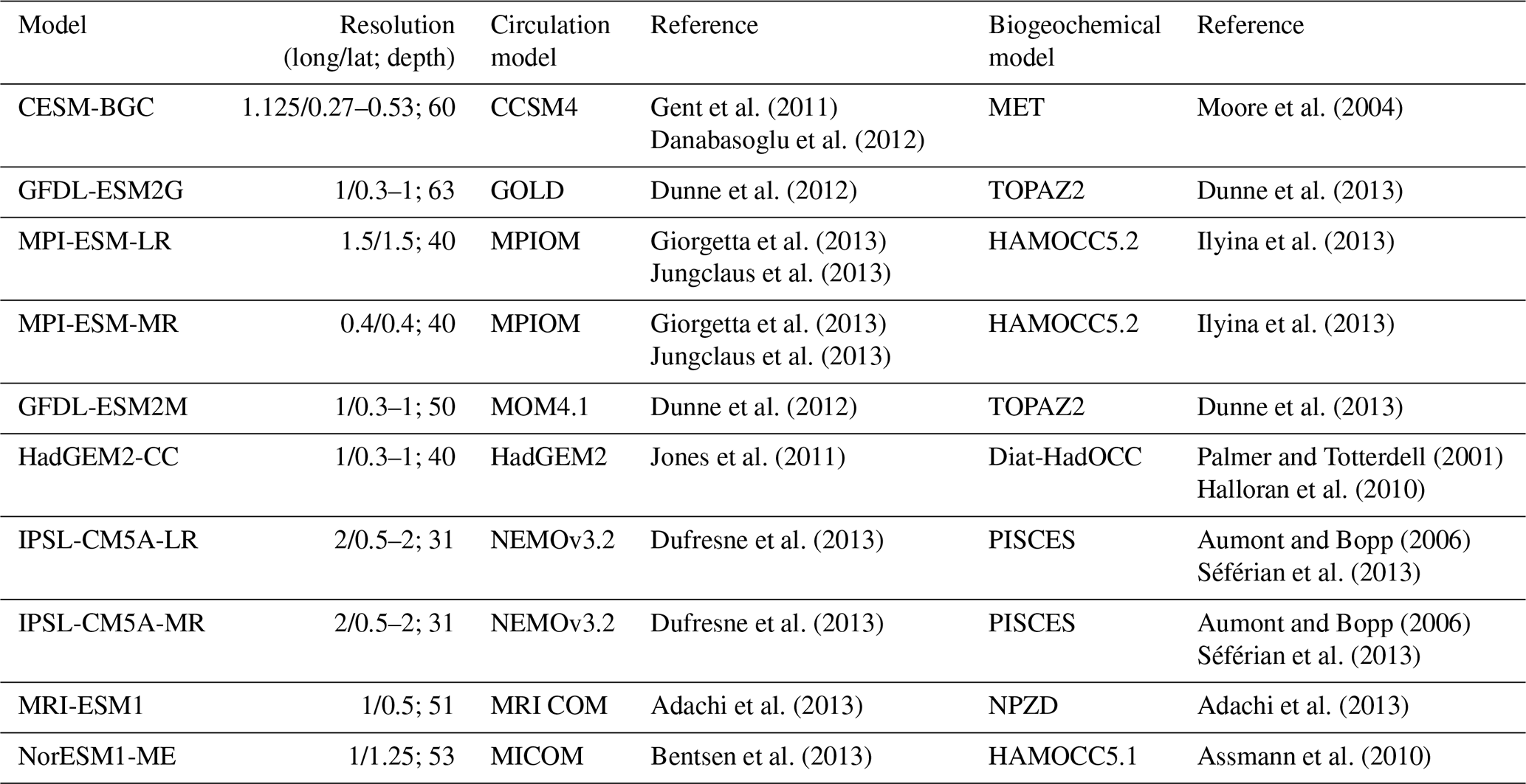
Gent et al. (2011)Danabasoglu et al. (2012)Moore et al. (2004)Dunne et al. (2012)Dunne et al. (2013)Giorgetta et al. (2013)Jungclaus et al. (2013)Ilyina et al. (2013)Giorgetta et al. (2013)Jungclaus et al. (2013)Ilyina et al. (2013)Dunne et al. (2012)Dunne et al. (2013)Jones et al. (2011)Palmer and Totterdell (2001)Halloran et al. (2010)Dufresne et al. (2013)Aumont and Bopp (2006)Séférian et al. (2013)Dufresne et al. (2013)Aumont and Bopp (2006)Séférian et al. (2013)Adachi et al. (2013)Adachi et al. (2013)Bentsen et al. (2013)Assmann et al. (2010)Table 1Summarized information on CMIP5 ocean model components and respective references. IPSL-CM5A-LR and IPSL-CM5A-MR differ only in the atmospheric horizontal resolution, with similar ocean modules in both model setups.
2.1 CMIP5 simulations
The Coupled Model Intercomparison Project (CMIP5; Taylor et al., 2012) framework was designed to identify strengths and weaknesses of Earth system models (ESMs) and thus improve climate predictions and identify uncertainties. In this study we included all ESMs from the CMIP5 project (Taylor et al., 2012) from which output of dissolved oxygen was available. The suite of these 10 model simulations includes results from the Community ESM (CESM-BGC), two versions of the Geophysical Fluid Dynamics Laboratory ESM (GFDL-ESM2G/M), the Hadley Centre Global Environment Model (HadGEM2-ES), two versions of the Institute Pierre Simon Laplace ESM (IPSL-CM5A-LR/MR), two versions of the Max Planck Institute ESM (MPI-ESM-LR/MR), the Meteorological Research Institute ESM (MRI-ESM1), and the Norwegian ESM (NorESM1-ME). For references and further details, see Table 1.
We focused on the so-called “historical” experiments that were conducted for the years 1850 to 2005. From this time period we extracted the years 1900 to 1999 and consider the averaged model results for further analyses. This period is long enough for a robust calculation of the climatological mean state. Averaging also ignores the seasonal cycle. The seasonal oxygen cycle is weak in the upper layers of the AS and not noticeable at greater depth (Schmidt et al., 2020). Thus, averaging is a reasonable approach for a uniform process analysis over large parts of the water column. Next to dissolved oxygen, temperature and salinity output from the same models was used in our analysis.
The CMIP5 ESMs differ in terms of the ocean circulation and biogeochemical modules. The horizontal resolution ranges from to , and the vertical resolution varies between 31 and 63 resolved depth levels. Table 1 gives an overview of the circulation and biogeochemical model components and their resolution. In order to compare the model outputs with the observations, all model outputs were re-gridded to the same grid on which the observational data are interpolated (see below).
2.2 Observations
For comparison with the model results we use the global dissolved oxygen, temperature, and salinity climatologies provided by the World Ocean Atlas 2013 (WOA13). The climatological annual mean data cover a period from 1955–2012 and are available with a spatial resolution of interpolated on 102 depth levels (Garcia et al., 2013; Locarnini et al., 2013; Zweng et al., 2013).
3.1 OMZ characteristics
As a first step, we compare the models and observations with respect to oxygen in the AS. Depending on the process of interest, it is likely that different oxygen thresholds and the corresponding water volume need to be investigated. We thus compare the volume of the ASOMZ for a range of thresholds from 0 to 100 µmol L−1. For a first spatial comparison, we chose our threshold to be 50 µmol L−1 to make it comparable to previous studies on CMIP5 oxygen distribution (e.g. Cabré et al., 2015; Cocco et al., 2013) and look at the horizontal extent of the ASOMZ as a function of depth and the actual location of these areas on a map.
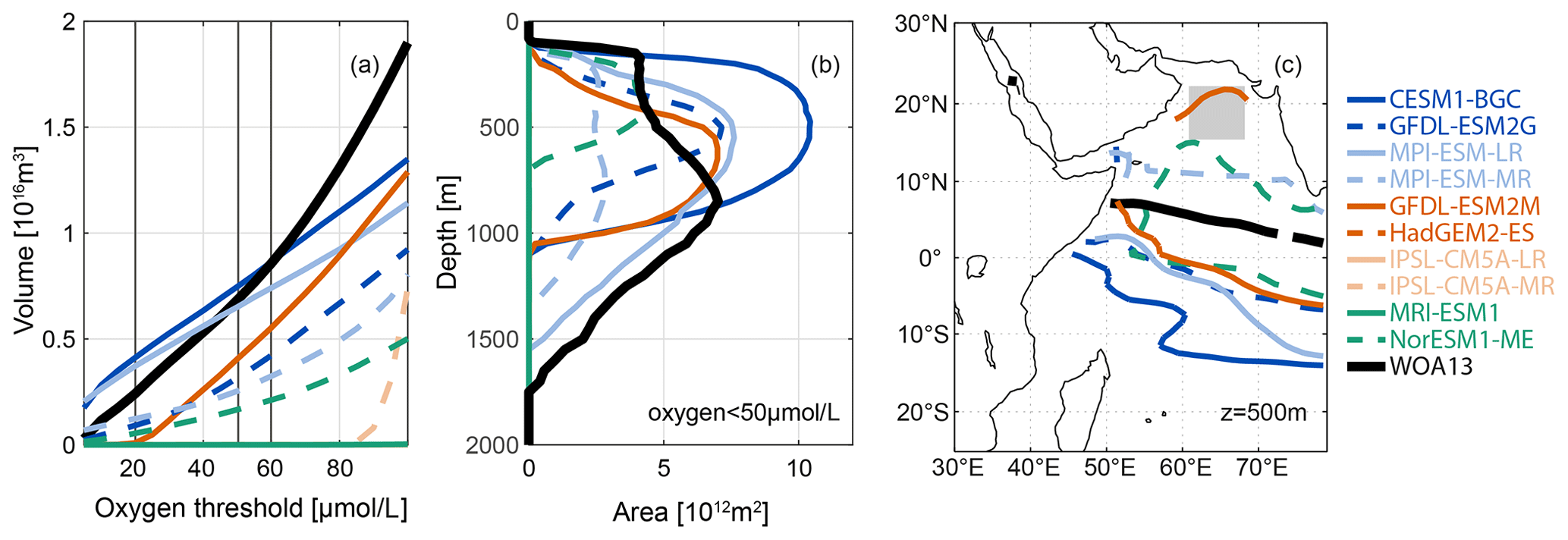
Figure 1Comparison of the Arabian Sea OMZ in observations (WOA13, black) and the CMIP5 models (coloured): (a) OMZ volume for different oxygen thresholds. The vertical grey lines mark the 50 µmol L−1 threshold for (b) and (c), as well as the 20 and 60 µmol L−1 thresholds that are discussed in the text. (b) Area of the OMZ for a threshold of 50 µmol L−1 at each depth. (c) Map of the OMZ area as defined in (b) at 500 m of depth. The grey box marks the area of the averaged vertical profiles shown in Fig. 5. Different colours refer to the different model clusters (see text).
3.2 Cluster analysis
To reduce the large amount of model output data and detect similarities between the models and observations we grouped them with hierarchical agglomerative cluster analysis (Johnson, 1967). Here, the correlation between the vertical oxygen profiles was used as the distance measure for the clusters. This means that profiles that are more similar to each other than to others are grouped together in a cluster. We are referring primarily to the curvature of the profiles and less to a systematic bias, e.g. an offset between profiles. For this purpose, the profiles are superimposed in such a way that the oxygen difference between the curves is minimal over the entire depth. This choice is motivated by the implicit assumption that the shape of the depth profiles contains more information on the underlying processes than the offset.
To determine the optimal number of clusters we used the silhouette criterion (e.g. De Amorim and Hennig, 2015). The silhouette is a common measure of how closely a certain data point (here a profile) matches the data within its cluster and how loosely it matches the data in the other clusters. A large value close to 1 implies that a data point is in the appropriate cluster, while negative values indicate a wrong cluster choice. We calculated the averaged silhouettes for three to six clusters and selected the number of clusters with the highest average silhouette value. The resulting best choice of four clusters meets our visual rating. We performed the cluster analysis for oxygen profiles in the AS for all 10 models considered in this study and the observations. Furthermore, we used the same clustering method for the salinity profiles. Salinity is a conservative tracer that is useful when investigating mixing of water masses. Clustering of the models with respect to the modelled oxygen and salinity profiles helped to find similarities between the models and gave hints for typical model problems in this dynamically complicated region.
For this analysis we chose to exclude coastal areas because the model bias in these areas is expected to be large due to the coarse resolution of the ESMs. We focus on the open-ocean core of the ASOMZ in the central AS between 16 and 22∘ N, 61 and 67∘ E, and from 10 to 1800 m of depth and analysed averaged profiles in this region, which is marked in Fig. 1c. To explain the differences between the models, these analyses were complemented by water mass mixing analyses and an analysis of the water mass properties in their formation region with respect to temperature, salinity, and oxygen.
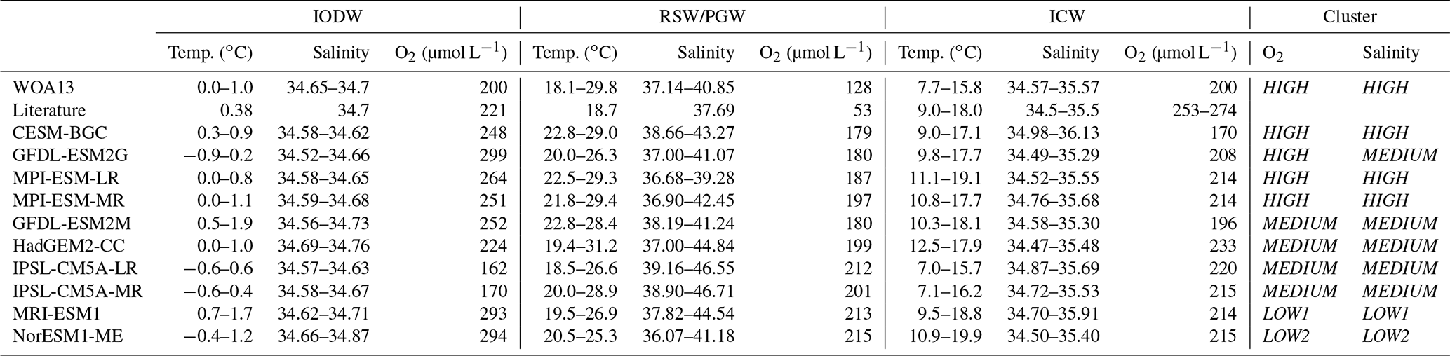
Table 2Overview of water mass characteristics in observations, the literature, and the CMIP5 models. Temperature and salinity values are given as upper and lower limits of the water masses. Oxygen is given as mean values. Literature values are taken from Hupe and Karstensen (2000; IODW, RSW/PGW) and Acharya and Panigrahi (2016; ICW).
3.3 Determination of water masses in models
Knowing the dominant water masses that mix in the ASOMZ, we analyse the representation of the respective water masses in the individual models. Therefore, we localized the formation regions of the water masses in observations (Figs. 2 and S1–S3). Red Sea Water and Persian Gulf Water (RSW/PGW) are geographically restricted in their formation regions. Figure 2a shows the formation region for RSW/PGW for which temperature and salinity ranges and mean values are determined (Table 2 and Fig. S4). In contrast, Indian Central Water (ICW) is not geographically restricted in its formation regions. ICW is a mixed water mass and is characterized by a nearly linear temperature–salinity relation that is density-compensated (Tomczak, 1984) and can be identified in T–S diagrams. With this relation, we were able to define upper and lower temperature and salinity limits of ICW in observations and compared those to respective values from the literature (see Table 2; Acharya and Panigrahi, 2016). ICW is formed along zonally oriented fronts in the tropical ocean subsurface layers (Tomczak, 1984). Sprintall and Tomczak (1993) and Schott and McCreary (2001) described the geographical location of the formation region of ICW. Figure 2b shows the grid boxes wherein these T–S properties are found in the IO in WOA13 observations. These are in line with the description of the formation region as shown by Sprintall and Tomczak (1993) and Schott and McCreary (2001). To investigate the formation region of ICW in the models, we followed the same procedure as previously described for the observations. The linear temperature–salinity relation as given by the T–S diagrams of the individual models (Fig. S5) sets the upper and lower temperature and salinity limits (see also Table 2 and Fig. S4c). In contrast to the observations and the literature, the resulting locations that determine the formation region of the simulated ICW are not restricted to the subduction area of ICW. For consistency we limit the formation region of ICW in the models to the subduction area of ICW as prescribed according to Sprintall and Tomczak (1993) andSchott and McCreary (2001): we exclude grid boxes with similar T–S properties that are found outside the subduction region. We also exclude grid boxes within the upper 200 m to analyse the oxygen content of permanently subducted ICW below the mixed layer depth that is transported to the AS and not re-ventilated into the seasonally varying well-ventilated mixed layer. Figure S2 shows the respective area for each model and the deepest depth at each location, where the T–S properties are found. Indian Ocean Deep Water (IODW) originates in the Southern Ocean, where it is often referred to as Circumpolar Deep Water and Antarctic Bottom Water, before it travels northward into the deep IO and mixes along its way with the surrounding water masses. IODW is thus defined as the densest water mass in the IO north of 60∘ S that is found below 1500 m of depth (Talley et al., 2011a, b). Figure 2c shows the formation region of IODW derived from observations. For this region temperature and salinity limits are determined. IODW in the models is defined in a similar way as in observations. In the models the derived formation regions of IODW in the Southern Ocean differ from those we find in observations (Fig. S3). The oxygen content of the water masses as listed in Table 2 and shown in Fig. S4 is calculated for each model and the observations by the arithmetic mean of all grid boxes of the corresponding source waters.
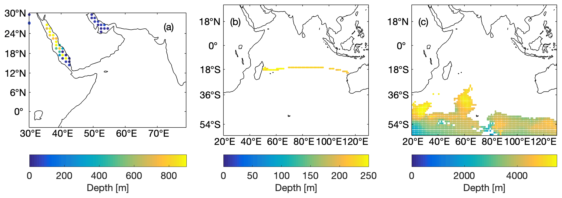
Figure 2Origins of the water mass formation regions from observations (WOA13) for (a) Red Sea and Persian Gulf Water, (b) Indian Central Water, and (c) Indian Ocean Deep Water. The colours indicate the deepest depth at each grid point wherein the respective water mass properties are found.
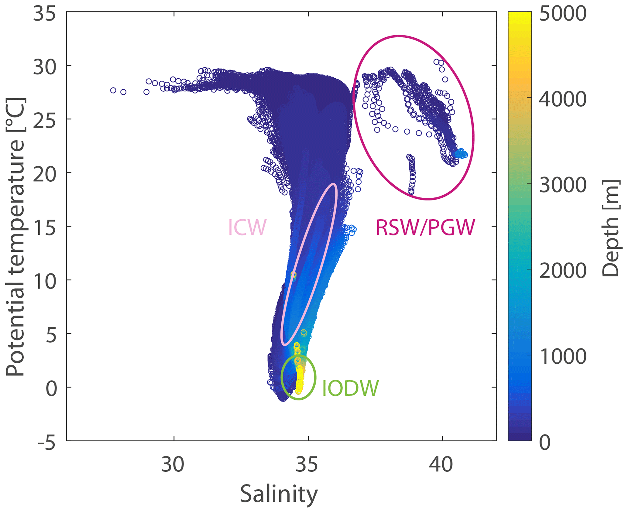
Figure 3T–S diagram of the Indian Ocean from observational data (WOA13) colour-coded by depth. The source water masses for the water mass mixing analysis are Indian Ocean Deep Water (IODW), Indian Central Water (ICW), and Red Sea and Persian Gulf Water (RSW/PGW). The ovals indicate the approximate T–S ranges of the respective water masses. Exact values of the water mass properties used in this study can be taken from Fig. 4 and Table 2.
3.4 Analysing uncertainties of water mass mixing ratios
As we want to understand the physical mechanisms controlling the oxygen distribution in the different clusters, we investigated the ventilation of the ASOMZ at different depths. Therefore, we carried out a water mass mixing analysis with the observations. This serves to identify the ventilation depth of the individual water masses and their contribution. The three main source water masses in the AS are IODW, RSW/PGW, and ICW (Fig. 3). We used a linear mixing approach and restricted the input to physical water mass properties from observational data. By considering potential temperature (θ), salinity (S), and mass conservation this yielded the possibility to resolve the mixing ratio of the three main source water masses in the AS. The set of linear equations is
where α, β, and γ are the mixing ratio coefficients for IODW, ICW, and RSW/PGW, respectively. The equations were solved at each data grid point.
We first solved the equations for each observational WOA13 data grid point in the box in the ASOMZ (Fig. 4b) by using observation-based temperature and salinity values of the source water masses from the literature (Table 2, Fig. 4a). Temperature and salinity values of the source water masses from the literature differ from those derived from the WOA13 observations. The same applies for the model temperature and salinity values. In addition, the properties of the water in the ASOMZ in the models differ from each other and from those of the observations. To obtain an uncertainty range of the water mass analysis that can be related to a change in the source water mass input, we solved the equations again for each observational WOA13 data grid point in the box in the ASOMZ, but this time we used arithmetic temperature and salinity mean values of the WOA13 data in the IO, following the calculations described in Sect. 3.3 for oxygen (Fig. 4c, d). This information about the sensitivity of mixing ratios to the definition of water mass properties allows us to draw conclusions on the significance of differences between modelled and observed mixing ratios. Note that the prescribed temperature and salinity values from the source water masses determine the vertical extent of the mixing results and limit our analysis to the central AS and thus the core region of the ASOMZ, which is the main interest of this study (Fig. 4b, d).
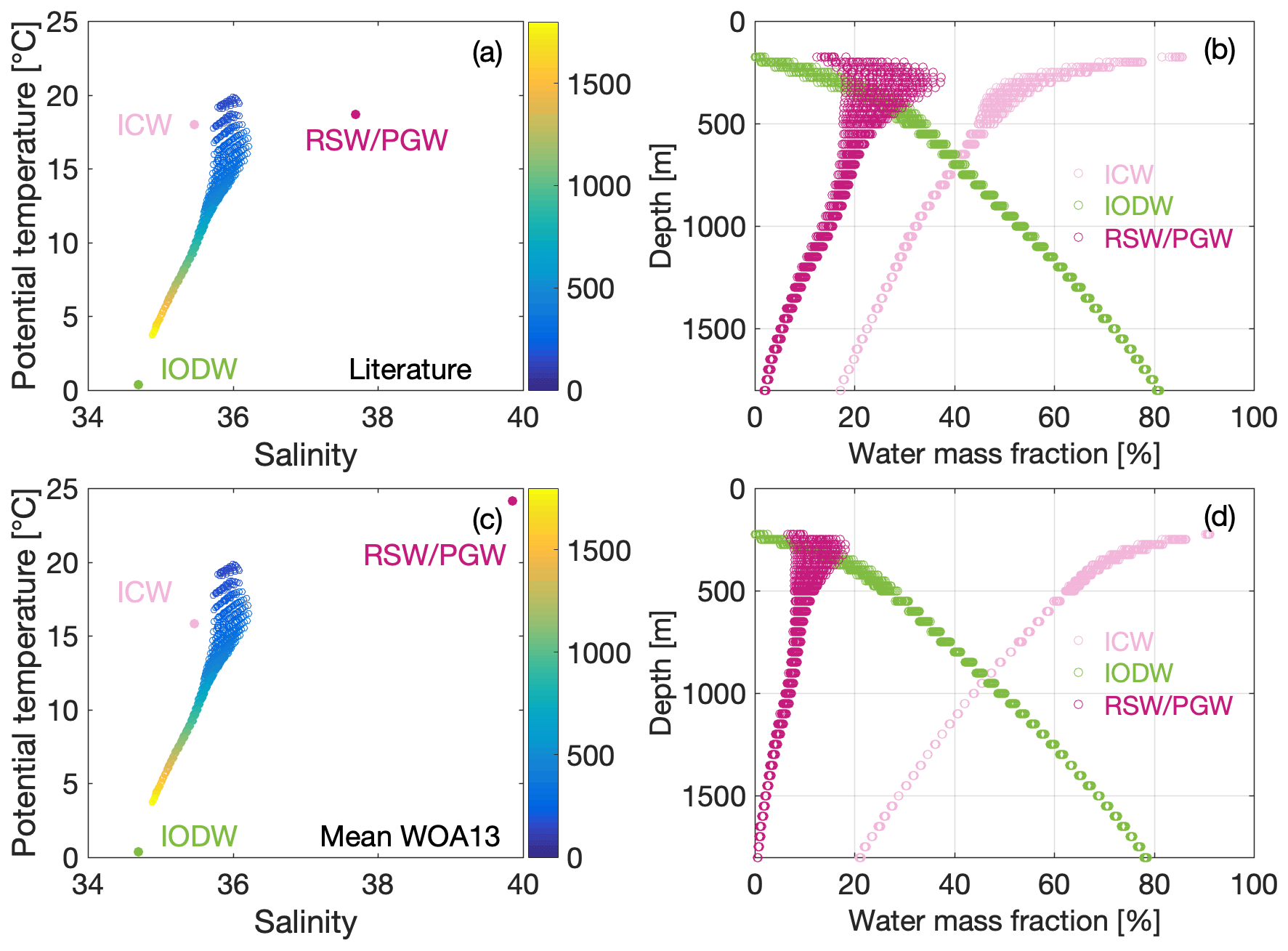
Figure 4T–S diagram of the Arabian Sea OMZ with the source water mass properties for the water mass mixing analysis (Indian Ocean Deep Water – IODW, Indian Central Water – ICW, and Red Sea and Persian Gulf Water – RSW/PGW) defined from (a) literature values and (c) the averaged observational data (WOA13) as well as the resulting water mass mixing fractures (b, d).
4.1 Comparison of observed and predicted OMZs in the CMIP5 models
For an overview of the differences in the oxygen distribution between models and observations, we calculated water volumes characterized by different oxygen thresholds in the AS westward of 79∘ E (Fig. 1a). Eight out of 10 models underestimate the volume of the ASOMZ for all thresholds and thus overestimate the oxygen content of the water.
Figure 1b shows the area integral for oxygen values below 50 µmol L−1 by depth. For the observations these areas can only be found between 200 and 1800 m of depth. The maximum horizontal extent of the ASOMZ amounts to around 900 m. Below 900 m all models underestimate the area, and thus oxygen concentrations themselves are overestimated compared to the observations. Above 900 m the models split into two groups; one group overestimates the horizontal extent of the ASOMZ and the other one underestimates it. To investigate this model–data misfit further we focus on the horizon at 500 m of depth, which is within the core of the OMZ in the models (Fig. 1c) and shows the largest model–data misfit. Four out of 10 models (IPSL-CM5A-MR,IPSL-CM5A-LR, HadGEM2-CC, MRI-ESM1) generally largely overestimate oxygen concentrations in that there is no water with oxygen concentrations less than 50 µmol L−1 at 500 m of depth (Fig. 1c). The models that overestimate the ASOMZ area of less than 50 µmol L−1 show oxygen values that are too low compared to observations in the whole AS and a southward expansion of the ASOMZ with one exception: in the NorESM1-ME model the ASOMZ is shifted to the southeastern boundary of the AS and is located between 15∘ N and the Equator (Fig. 1c). All in all this wider horizontal expansion of the oxygen-poor areas (oxygen < 50 µmol L−1) in the models compared to the observations (Fig. 1c) cannot compensate for the reduced thickness of the low-oxygen layers, which is responsible for the general underestimation of the ASOMZ volume in the CMIP5 models (Fig. 1a).
Thus, the oxygen distribution differs considerably among the CMIP5 models in the AS. None of the CMIP5 models reproduce the observed oxygen distribution. Also, the volume of the ASOMZ depends highly on the threshold (Fig. 1a). For a more general comparison of the models with each other and with the observations, we therefore decided to use averaged oxygen profiles in the AS for the cluster analysis.
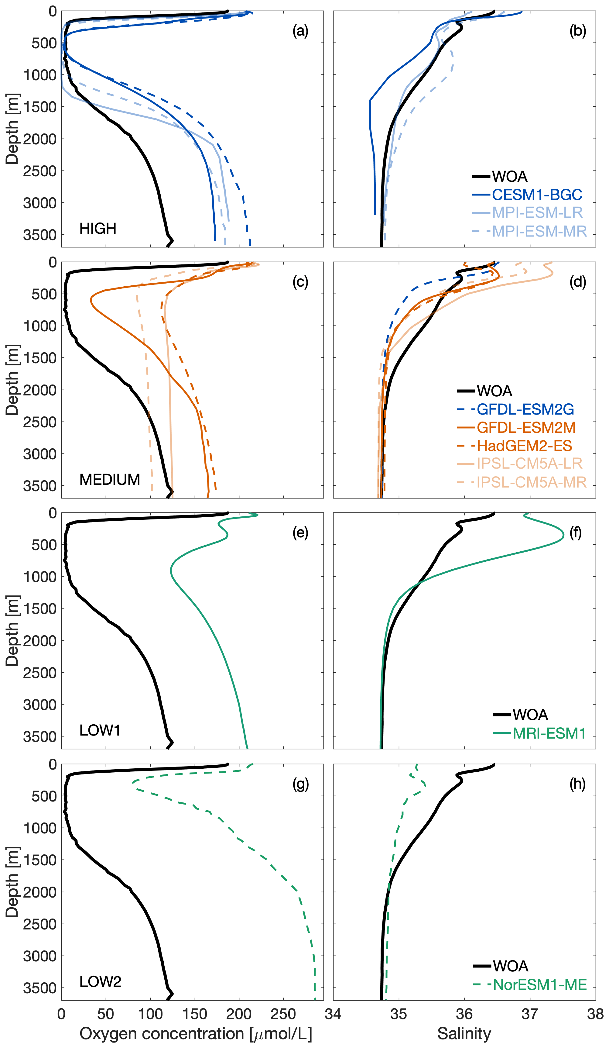
Figure 5Averaged vertical oxygen (left) and salinity (right) profiles in the box between 16–22∘ N and 61–67∘ E (see Fig. 1) in the Arabian Sea for CMIP5 models (coloured) and observational data (black). Blue-coloured models belong to oxygen cluster HIGH (a–b), red to cluster MEDIUM (c–d), and green to clusters LOW1 (e–f) and LOW2 (g–h).
4.2 Cluster analysis
We performed a cluster analysis to identify commonalities between the models. Figure 5 shows these profiles averaged over the box in the core region of the ASOMZ as shown in Fig. 1c. Based on the silhouette criterion (see Sect. 3.2) we obtain the first four oxygen clusters. The naming of the clusters is based on their agreement with the observations. Cluster HIGH groups with the observations and contains the CESM1-BGC, GFDL-ESM2G, and MPI-ESM-MR/LR. Cluster MEDIUM contains the HadGEM2-CC, GFDL-ESM2M, and IPSL-CM5A-MR/LR. In addition, two outliers were identified that each form their own cluster: MRI-ESM1 (cluster LOW1) and NorESM1-ME (cluster LOW2).
At the surface in the AS all models show an oxygen concentration that is about 25 µmol L−1 higher than in observations (Fig. 5a, d, e, g), and also below 1800 m all models (except IPSL-CM5A-MR) overestimate oxygen concentrations (Fig. 5a, d, e, g). The main difference between the clusters is noticeable between 250 and 1300 m of depth in the core of the ASOMZ, where observed oxygen concentrations are close to zero. Although cluster HIGH models show averaged oxygen concentrations close to zero, not all cover the full depth range of the observed ASOMZ core (Fig. 5a). Cluster MEDIUM models generally show higher averaged oxygen concentrations above 80 µmol L−1 (Fig. 5c) in comparison to cluster HIGH. The model of cluster LOW1 has even higher oxygen concentrations (Fig. 5e), and the model of cluster LOW2 has an averaged oxygen minimum that is found at shallow depths around 400 m (Fig. 5g).
To differentiate between physical and biogeochemical processes responsible for the model–data misfit, we also performed the cluster analysis for the averaged salinity profiles. The results show that only the GFDL-ESM2G changes from oxygen cluster HIGH to salinity cluster MEDIUM; all other models are grouped in the same clusters compared to the oxygen cluster analysis (Fig. 5b, d, f, h). Below 1800 m the simulated averaged salinity profiles (Fig. 5b, d, f, h) are close to observations. Between 800 and 1800 m 9 out of 10 models underestimate the salinity. Differences in overestimation and underestimation of salinity in the upper 800 m characterize the individual clusters. Three out of four cluster HIGH models overestimate the salinity up to the upper boundary of the ASOMZ (Fig. 5b). In contrast to that all cluster MEDIUM models overestimate the averaged salinity at depths around 400 m (Fig. 5d). Cluster LOW1 has even higher salinity values than the models from cluster MEDIUM. The model of cluster LOW2 underestimates the salinity all the way up to the surface (Fig. 5h).
The clustering reveals a connection between the representation of oxygen and salinity in the CMIP5 models with one exception (GFDL-ESM2G). The grouping of the models of cluster HIGH with the observations indicates that the circulation in this group is similar to the real circulation, or at least that we could not identify any fundamental problems in the modelled circulation. Still, the ASOMZs of the models of cluster HIGH differ in shape and extent compared to the observed ASOMZ. The results further indicate that in clusters MEDIUM, LOW1, and LOW2 model deficiencies in the circulation models are responsible for deficiencies in the oxygen representation. In addition to the uncertainties in the physical model component these models can also have deficiencies in the biogeochemical model components. These are just not clearly identifiable due to the underlying uncertainties in the physical model components.
4.3 Water mass representation in models
Differences in the physical model component, e.g. the representation of water masses (including mixing), seem to be the key process that determines the affiliation of a model with a certain cluster. In the following, we concentrate on the three main water masses that mix in the ASOMZ, which are IODW, ICW, and RSW/PGW. The water mass mixing analysis (Fig. 4) shows that IODW is the dominating water mass in the deep AS. Above ∼ 900 m, the impact of ICW and RSW/PGW on the ASOMZ dominates. The underlying uncertainties, which include the percentages of the individual water masses with depth, are explained in detail in Sect. 4.4.
IODW forms in the Southern Ocean, where it is often referred to as Circumpolar Deep Water. Its temperature varies from 0 to 1 ∘C and its salinity from 34.65 to 34.7 (Table 2 and Fig. S4a). All models reproduce these characteristics fairly well. Also, the formation region (Figs. 2c and S3) is correctly simulated by all models. The only exception is NorESM1-ME. In this model the properties of IODW do not reach deep enough in the southern IO and a large amount can be found in the eastern equatorial IO.
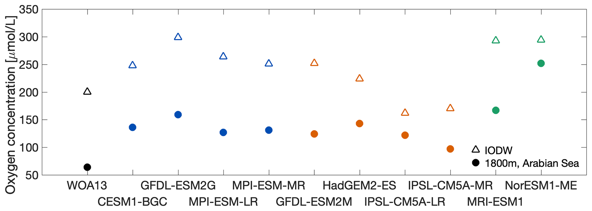
The simulated oxygen concentrations of IODW vary between 181 (IPSL-CM5A-MR) and 301 µmol L−1 (NorESM1-ME; Table 2 and Fig. 6). The observational mean oxygen concentration is 200 µmol L−1 (Table 2, Fig. 6). Figure 6 shows a comparison of the oxygen concentrations at the bottom of the ASOMZ at 1800 m of depth and of IODW in its formation region. The difference between those two concentrations indicates that the respiration of organic matter during the transit from the formation region of IODW to the central AS results in an oxygen consumption of 136 µmol L−1 in the observations. In clusters HIGH and LOW1, all models show oxygen concentration differences between IODW and the bottom of the ASOMZ that are similar to the one found in the observations. However, the resulting simulated oxygen concentrations still differ quite substantially. Here it is important to note that the modelled IODW shows an almost systematic oxygen offset in the Southern Ocean (Fig. 6). For the majority of cluster MEDIUM models (IPSL-CM5A-MR/LR, HadGEM2-CC) and cluster LOW2 the oxygen concentration difference is smaller compared to the one in observations. This indicates uncertainties in the oxygen consumption in the abyssal ocean.
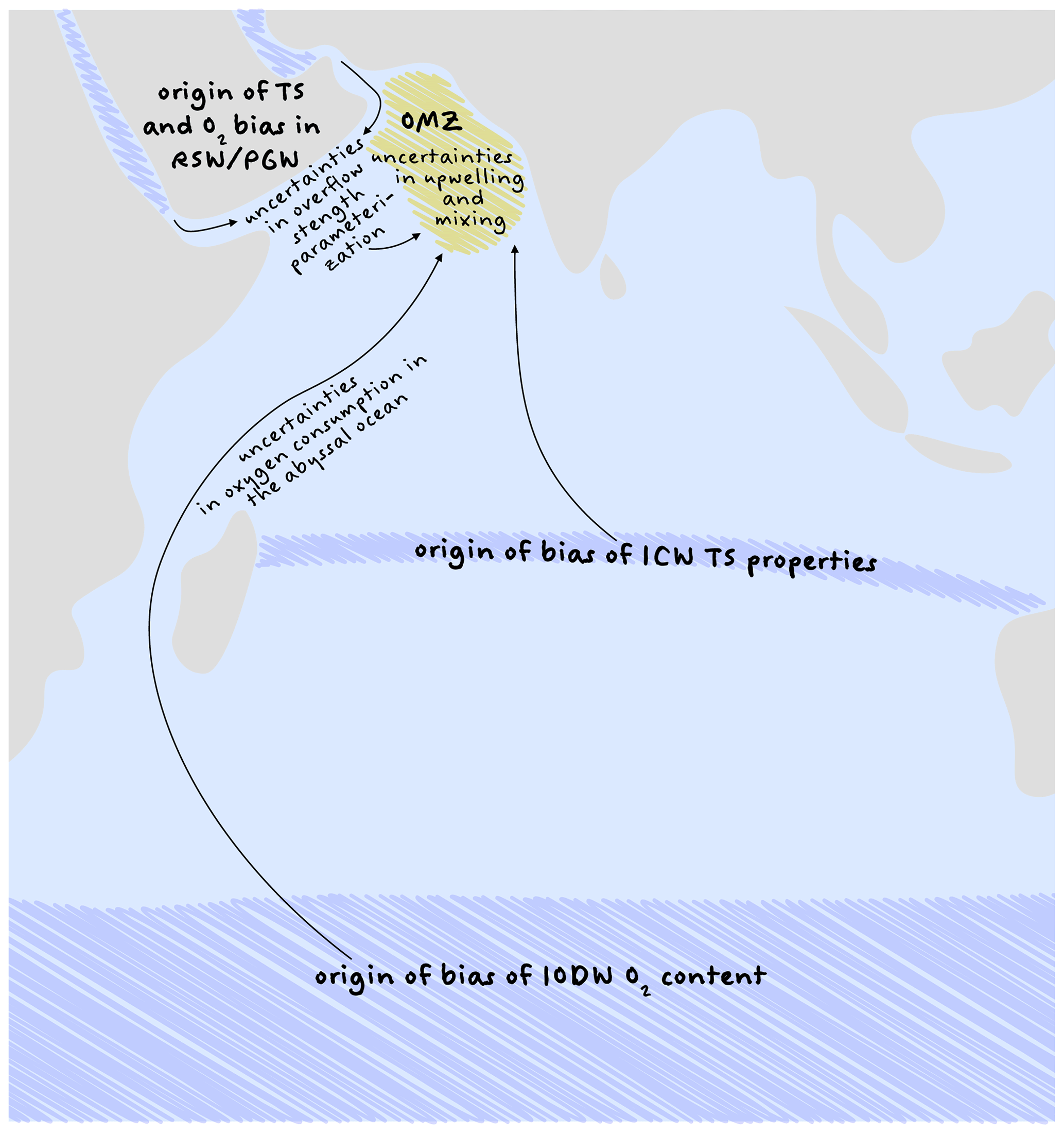
Figure 7Overview sketch of the analysed origins of model–data misfits in oxygen in CMIP5 models. The blue shaded areas mark the origins of the water masses and their related biases in the models. The arrows sketch the way into the OMZ and uncertainties on the way. The yellow shaded area sketches the OMZ in the Arabian Sea.
Differences in the transit time can be determined by an age tracer. Only 2 out of 10 models include an ideal age, which is an idealized tracer that counts the time since the last surface contact. We obtained the ideal age of IODW in the Southern Ocean by the arithmetic mean of all grid boxes of the formation region of the source water mass, similar to the calculation of the oxygen content (Sect. 3.3). In the deep AS the ideal age is calculated by the mean within the averaging box of the profiles (Fig. 5) below 1800 m of depth. The GFDL-ESM2G (cluster HIGH) has an average ideal age of 101 years of IODW in the formation region in the deep Southern Ocean and an average age ideal of 579 years in the deep AS (Fig. S6). In the GFDL-ESM2M (cluster MEDIUM) the respective ideal ages are older with 252 and 780 years, respectively (Fig. S6). The age differences between the formation region and the AS are 478 years (GFDL-ESM2G) and 528 years (GFDL-ESM2M). This shows that the water mass age in the source region of the two models differs, which already might explain the lower oxygen concentration of GFDL-ESM2M in the Southern Ocean.
In addition, both models have the same biogeochemical model component and the same horizontal resolution of the physical model component, but they differ in their vertical resolution (Table 1). Differences in the ideal age in the source regions of IODW between these two models indicate that the vertical resolution has an impact on the water mass formation process in the Southern Ocean. Differences in the transit times indicate that the circulation differs among the two models, also as a result of the differences in the vertical resolution. In addition, export production might also be affected by changes in the vertical model resolution.
RSW and PGW are straightforward to define in models, as they have a distinct origin in the Red Sea and the Persian Gulf, respectively (Figs. 2a and S1). The observed temperature range between 18 and 30 ∘C is well represented in all models (Table 2 and Fig. S4b). However, the simulated salinity in the formation region varies among the models. While the lower limit of 37.14 in observations is met by most models (Table 2 and Fig. S4b), the upper limit varies from 39.28 (MPI-ESM-LR) to 46.71 (IPSL-CM5A-MR). In general, we find an overestimation of the salinity of RSW/PGW in all clusters. Consequences of more saline, and thus denser, water are a ventilation of the ASOMZ at incorrect depth levels and model artificial salinity maxima.
The averaged salinity profiles in the AS confirm this overestimation of salinity, especially for cluster MEDIUM (LOW1) between 200 and 500 m (1000 m) of depth (Fig. 5d, f). For cluster LOW1 the deep-reaching salinity overestimation cannot be explained by offsets in the source water mass properties alone, although the peak at around 500 m of depth coincides with the depth of maximal water mass contribution of RSW/PGW (Fig. 5f). A possible further explanation would be enhanced mixing of RSW/PGW into the AS and also stronger evaporation and/or less precipitation over the AS. Below 500 m, the reduced salinity and the mixing analysis indicate less input of RSW/PGW in nearly all models compared to observations. This deficit would therefore have to be compensated for by another water mass that is mixed into the ASOMZ. The mean oxygen content of RSW/PGW is quite similar among the models but has a considerable positive offset compared to observations of up to 87 µmol L−1 (Table 2 and Fig. S4b). While the observations show a mean oxygen content of 128 µmol L−1, the models range from 179 (CESM) to 215 µmol L−1 (NorESM1-ME). The oxygen concentration differences between the clusters are comparable to those within the clusters, even though the models in cluster HIGH tend to have lower oxygen concentrations than those in cluster MEDIUM. The enhanced oxygen concentrations in the ASOMZ in cluster MEDIUM can be explained by the higher oxygen concentrations in the formation region of RSW/PGW combined with the modified mixing of water in the ASOMZ due to density changes by overestimated salinities of RSW/PGW (Fig. 5c, d). In clusters LOW1 and LOW2, RSW and PGW have the highest oxygen concentration of all models.
ICW is subducted in the southeastern IO in the subtropical cell region (Figs. 2b and S2). Central water masses can be recognized by their linear T–S relationship. Table 2 and Fig. S4c give the upper and lower temperature and salinity limits of ICW for each model. The observational temperature range (7.7–15.8 ∘C) is 2.2 ∘C below the established literature value. The temperature range of the models thus corresponds to those values ranging from 7 ∘C (IPSL-CM5A-LR) to 19.9 ∘C (NorESM1-ME). Also, the salinity corresponds to a great extent to values from 34.57 to 35.57 in observations and 34.49 (GFDL-ESM2G) to 36.13 (CESM-BGC) in models. For both properties the clusters show no clear separation among each other (Table 2).
The mean oxygen concentration of ICW of the models spreads from 170 µmol L−1 (CESM-BGC) to 233 µmol L−1 (HadGEM2-CC), which brackets the observational concentration of 200 µmol L−1. Again, no clear separation between the clusters is noticeable.
4.4 Uncertainties of water mass mixing ratios impacting the OMZ according to observations
We performed the water mass analysis for the observations for two different sets of the source water mass properties. The first set comes from established literature values (see Table 2 for values and references as well as Fig. 4a). The second set is derived from WOA13 data (Fig. 4c; Sect. 3.4). This enables us to estimate the sensitivity of the analysis related to differences in water mass characteristics in the source regions.
Starting with the literature values, the impact of IODW on the lower ASOMZ dominates with a contribution of up to 80 % (Fig. 4b). IODW still has an impact of about 50 % at intermediate depths below 800 m, but is barely found at the upper boundary of the ASOMZ at 200 m. Above ∼ 900 m ICW and RSW/PGW dominate (Fig. 4b). In particular, the ICW has a maximum contribution of about 80 % at the upper boundary of the ASOMZ that decreases downward to a fraction of less than 20 % at 1800 m of depth. Above 500 m of depth RSW and PGW contribute between 15 % and 40 % to the mixed water in the ASOMZ (Fig. 4b). This fraction decreases with depth, tending towards 0 % at the bottom of the ASOMZ.
The spatial variability of the composition of water masses is more variable in the upper layers of the ASOMZ. This is due to the fact that temperature and salinity in the deep ocean vary less than in the thermocline, affected by heat and freshwater fluxes, seasonal variations, and turbulent mixing.
Switching to the source water mass definitions based on the WOA13 data (Fig. 4c; Sect. 3.4), the greatest deviation of the input parameters is for RSW/PGW (Fig. 4a, c). The mean temperature values of this water mass of 24.1 ∘C are 5.4 ∘C higher and the mean salinity values of 38.9 are 2.2 higher compared to the literature values of Hupe and Karstensen (2000). The ICW temperature derived from the mean WOA13 data is 15.8 ∘C and thus lower than the literature value of Acharya and Panigrahi (2016).
The mixing ratios for IODW derived from the WOA13 data (Fig. 4d) are similar to those obtained from the literature values. The impact of ICW on mixing ratios in the ASOMZ is generally a few percent higher throughout the water column for the WOA13 data compared to the literature values. The largest differences, however, are noticeable for RSW/PGW at depths between 200 and 600 m, where the maximum contribution is 20 % with WOA13 input. This is just half as much RSW/PGW that mixes into the ASOMZ as when literature values are used to define the water masses.
Comparing the outcome of these two water mass analyses gives a stable result for the mixing of water masses in the deep AS. Furthermore, the results are particularly sensitive to variations in RSW/PGW characteristics. As seen in Sect. 4.3 RSW/PGW is by far the saltiest and warmest water mass, but also its T–S properties show largest variations across the different models. This can result in uncertainties in the mixing ratio of the water masses in the models in the ASOMZ. Since the water masses are of different origins and also have different oxygen concentrations, different mixing ratios can affect the simulated oxygen content of the OMZ.
CMIP5 models do not represent the ASOMZ very realistically. In the core region of the ASOMZ the averaged oxygen profiles exclusively display higher oxygen concentrations in the models than in observations (Fig. 5a, c, e, g). Our findings for the AS cannot support previous global and regional studies pointing out that CMIP5 models systematically overestimate the volume of OMZs (e.g. Bopp et al., 2013 – global OMZs; Cabré et al., 2015 – Pacific OMZs; threshold of 50 µmol L−1). For a more detailed comparison of simulated and observed ASOMZs, it is useful to investigate the model behaviour for a range of different thresholds, as the models behave differently at different thresholds. Eight out of 10 models underestimate the ASOMZ volume for all thresholds < 100 µmol L−1 (Fig. 1a). Two models (CESM1-BGC, MPI-ESM-LR) overestimate the ASOMZ volume when considering oxygen < 60 and < 50 µmol L−1, respectively, and underestimate it for higher oxygen thresholds. This is in line with Rixen et al. (2020), who show an ASOMZ volume twice as high as observed for CESM1-BGC and MPI-ESM-LR for oxygen < 20 µmol L−1.
The general underestimation of the ASOMZ volume is mainly caused by a vertical extent of the OMZ that is too small (Fig. 1b). Previous studies (e.g. Kamykowski and Zentara, 1990; Rao et al., 1994) that included observations pointed out that the core with oxygen values below 5 µmol L−1 expands over a depth range of about 1000 m. The vertical expansion of the horizontally confined ASOMZ is especially important for a good volume representation. However, only 1 in 10 models is able to completely cover this depth of oxygen-depleted water (MPI-ESM-LR; Fig. 5a).
To simulate the ASOMZ accurately, both the physical (ventilation) and biogeochemical components (respiration) must be adequately represented in the models. Starting with the water masses that contribute to the ASOMZ, errors in water mass formation and transport can result in an incorrect representation of the ASOMZ. A major CMIP5 model problem that we could identify is the higher-than-observed oxygen content in the Southern Ocean, which is reflected in the deep AS. We find this tendency in all models and there is no cluster dependency (Fig. 6). To further explain this higher-than-observed oxygen content in the Southern Ocean, the formation of IODW must be considered. Therefore, it is meaningful to use and discuss not only Circumpolar Deep Water (CDW) but also Antarctic Bottom Water (AABW) as a source for IODW. First, this is reasonable because the water mass properties of CDW (1.85 ∘C, 34.69; multi-model mean from Sallée et al., 2013b) and AABW (0.18 ∘C, 34.72) overlap our and the literature definition of IODW. Second, the term IODW is often only used in the AS, and CDW and AABW both flow along the western margin towards the north and could thus mix on the way to become IODW. Assuming that the IODW in the models is formed to a large extent from AABW and not from CDW as actually described in the literature (Schott and McCreary, 2001), this could explain the higher-than-observed oxygen content in the Southern Ocean IODW because AABW should be recently ventilated and generally younger than CDW, and it thus contains more oxygen. Sallée et al. (2013b) find large variations in AABW volume of the individual models, and their multi-model mean volume exceeds the one estimated from observations (5.5×10¹⁶ m3), which supports our assumption. Two models, one of cluster HIGH (GFDL-ESM2G) and the model of cluster LOW2 (NorESM1-ME), overestimate the volume of AABW by far ( m3). We identify no clear differences in volume of AABW as found by Sallée et al. (2013b) between the individual clusters of our study (e.g. the volume of AABW in MPI-ESM-LR – cluster HIGH – and in HadGEM2-CC – cluster MEDIUM – is nearly similar with m3), which coincides with the cluster-independent oxygen overestimation.
Furthermore, Sallée et al. (2013b) find that all models, with one exception (HadGEM2-CC), underestimate the volume of CDW with a multi-model mean volume of 25.2×10¹⁶ m3, which corresponds to about 77 % of the observed volume. If we look at the CDW volume of the individual models considered in our study, most of the models, independent of the clusters, have a volume of CDW that is just below the multi-model mean volume of Sallée et al. (2013b). This excessive amount of AABW along with the smaller volume of CDW in the models could explain the higher-than-observed oxygen content in the Southern Ocean in all clusters.
For the models of clusters HIGH and LOW1 we see this positive oxygen offset in the Southern Ocean propagating into the deep AS (Fig. 6). However, the models of clusters MEDIUM and LOW2 show smaller-than-observed oxygen differences between the formation region of IODW in the Southern Ocean and the bottom of the ASOMZ (Fig. 6). This smaller oxygen difference could be explained by different ventilation pathways and timescales of IODW on the way northward into the ASOMZ and associated less cumulative oxygen consumption on the way. The comparison of the two GFDL ESMs (clusters HIGH and MEDIUM), which have the same biogeochemical model component, shows a difference in the ideal age in the Southern Ocean of 150 years and in the deep AS of 50 years. (Fig. S6). This suggests that the circulation differs in both models and thus also the transit time, which would influence the cumulative consumption rate on the way northward from the Southern Ocean.
A possible explanation for these uncertainties of the deep-ocean circulation and water mass properties in the models is the generally coarse vertical resolution there that shapes the bottom topography and limits biogeochemical processes related to the benthopelagic ecosystem (Kwiatkowski et al., 2020). The coarse resolution can influence the export pathways and thus timescales of IODW, and the benthopelagic ecosystem defines the oxygen consumption rate on its way and causes oxygen concentration differences in the deep AS. Based on the ventilation time differences in clusters HIGH and MEDIUM and the oxygen differences between the Southern Ocean and the AS (Fig. 6), it can be suggested that in clusters MEDIUM and LOW2, circulation is responsible for a large part of the oxygen differences in the deep ASOMZ, since the models of cluster HIGH are closer to the observations.
In addition, we also find uncertainties in the models in the formation regions of the other ventilating water masses. In the models RSW/PGW oxygen concentrations show a huge positive offset compared to observations. The observations show a strong decrease in oxygen from around 200 µmol L−1 at the surface down to 50 µmol L−1 in 300 m of depth. This oxygen decrease is only captured by two models (CESM1-BGC, GFDL-ESM2G). In the other eight models, oxygen is uniformly distributed throughout the water column. A possible reason for this model–data oxygen difference in RSW/PGW could be the poor resolution of coastal regions and shelf areas in the coarse-resolution models, which includes the shallow marginal seas. It is also noticeable that the solubility of RSW/PGW is higher in 6 of the 10 models compared to observations (Table S1). This is another possible reason for a positive oxygen offset.
Furthermore, coarse-resolution models generally prescribe the overflow through small channels that are not resolved by the grid resolution. This is also the case for the outflow of RSW/PGW. Seland et al. (2020) find a core in the AS that is too warm and saline at subsurface depth in the CMIP6 version of the NorESM and trace it back to the outflow of the Red Sea. They state that such subsurface ocean biases can be linked to the coarse ocean resolution and deficiencies in process parameterization. We can find similar patterns in our study with a saline layer that is too saline in clusters MEDIUM and LOW1 above 500 m of depth (Fig. 5d, f), which is likely caused by the inflow of RSW/PGW. This points towards a problem in the parameterization of the outflow of RSW/PGW at least in the clusters MEDIUM and LOW1. In addition, the higher-than-observed salinity could be strengthened by the positive salinity offset in models compared to observations in the source regions of RSW/PGW, which we found in all clusters. Somewhat surprisingly, 8 of 10 models from all clusters show less-saline water than the observations in the layer between 500 and 1800 m of depth (Fig. 5b, d, f, h), which might be explained by overestimated ventilation with ICW.
ICW, the other intermediate water mass that ventilates the ASOMZ, is subducted in the subtropical cell region in the southeastern IO. Propagating westward and northward into the AS, it likely mixes with other intermediate water masses in the subtropical and tropical IO. The models considered here show water mass characteristics that fit the observations within the area where ICW is permanently subducted. Our results do not agree with those of Sallée et al. (2013a, b), who examine the circulation and water mass formation in CMIP5 models in the Southern Ocean. They found a warm bias in the subtropical region in nearly all models and a seasonal cycle of the subtropical mixed layer that is too strong, which causes excess subduction of mode water that is too light in the western basin that gets denser in the eastern part of the basin. Sallée et al. (2013b) further state that the total amount of subtropical water in the models is underestimated. However, our mixing analysis indicates that the ASOMZ is ventilated to a larger extent by ICW in the models than in the observations. We thus consider it necessary to further investigate the various subtropical and tropical IO water masses in CMIP5 models and their formation processes before giving a clear statement about the mixing amount and the properties of ICW when it reaches the ASOMZ.
Recent studies by Séférian et al. (2020) and Kwiatkowski et al. (2020) analysing CMIP5 and CMIP6 model data show that increasing the horizontal resolution of the ESMs from non-eddy-resolving to eddy-permitting does not overcome the major problems with respect to realistically simulating oxygen in the open ocean. Despite better representation of mesoscale processes due to the higher resolution, the expected improvement in oxygen representation is absent in the CMIP6 models on a global scale (Séférian et al., 2020). Inclusion of mesoscale processes in the CMIP6 models resulted in only moderate improvements in subsurface oxygen representation (Kwiatkowski et al., 2020). While the model–data misfit for the upper-ocean oxygen content was reduced from the CMIP5 to CMIP6 model versions in the Indian and Pacific Ocean, Séférian et al. (2020) suspect a systematic bias in biogeochemical models due to sign shifts in model–data deviations between the two CMIP phases in the Atlantic Ocean, where the CMIP5 models simulated a stronger-than-observed OMZ and the CMIP6 models a weaker-than-observed OMZ. Among the non-eddy-resolving CMIP5 models considered here, we confirm the lack of an apparent systematic coherence between model resolution and better representation of the ASOMZ (Tables 1 and 2). This is not what we expect from the results of regional eddy-resolving models, i.e. that ventilation of the ASOMZ occurs through mixing processes mainly related to mesoscale eddies (e.g. Resplandy et al., 2012; Lachkar et al., 2016). An increased horizontal resolution of the model should therefore lead to more explicitly resolved mesoscale eddy activity, which might allow for more ventilation and thus a change in the ASOMZ. It seems that resolving mesoscale eddies leads to substantial improvements in the representation of the ASOMZ (Resplandy et al., 2012; Lachkar et al., 2016). However, moving from the range of non-eddy-resolving models to eddy-permitting models, a higher resolution seems to have a minor effect on the ASOMZ.
In addition, Kwiatkowski et al. (2020) and Tagklis et al. (2020) state that the spin-up times of CMIP5 models are not long enough to equilibrate biogeochemical conditions in the deep ocean. Mignot et al. (2013) show that physical properties and the large-scale circulation are already in equilibrium after 250 years, whereas Séférian et al. (2016) show that this does not hold for biogeochemical tracers. Moreover, the drift is highly model-dependent and not directly correlated with the spin-up times that range from 500 (HadGEM2-CC) to 11 900 years (MPI-ESM-LR). In our study we also cannot find a connection between the model spin-up times and the oxygen change during the 20th century in the AS and the ASOMZ representation in the historical experiment of the models, especially not in the deep AS (Fig. S7). Nevertheless, there are also opposing oxygen trends in the deep AS in all models between 1900 and 1999, but they are small (−2.5 to 2 µmol L−1) compared to the trends in the thermocline and the OMZ layer (−6 to 10 µmol L−1; Fig. S7).
In the cluster analysis, offsets in oxygen concentrations between profiles were not considered (Fig. 5a, c, e, g). We focused rather on the shape of the curves because we regarded the information content as higher for our purposes. The oxygen overestimation of all the considered models at the surface in the AS can be explained by higher oxygen solubilities at the surface in the models of up to 4.7 % compared to observations (Table S1). These higher solubilities are caused by lower-than-observed temperatures in the models at the surface (Fig. S8). With the higher solubilities and the positive oxygen offset at the surface in the models, more oxygen could be mixed into the ASOMZ from above than in the observations. Mixing of oxygen from the surface to the interior ocean is dependent on the stratification in the upper ocean as well as the oxygen gradient. The averaged stratification over the box in the AS in the models strongly resembles the observational stratification (Fig. S9). Furthermore, all models and the observations show a strong oxygen gradient above the ASOMZ. Thus, it is possible that a small proportion of the overestimated oxygen concentrations in the models could be explained by solubility differences at the surface of the AS.
What has not yet been taken into account in this analysis and might influence the supply of oxygen from below to the ASOMZ are possible deficiencies in upwelling in the AS. Upwelling of oxygenated deep and bottom water that is too strong from below would flatten and weaken the ASOMZ. You (2000) and Stramma et al. (2002) find a deep overturning circulation in the AS with inflow below 2500 m of depth and an overlying outflow between 300 to 2500 m of depth. Stramma et al. (2002) state that the rising bottom water in the AS reduces its oxygen content by mixing with the less-oxygenated intermediate waters. However, they point out that there are large uncertainties associated with computing the strength of the overturning cell. Thus, there is no reference value for upwelling strength in the AS we could compare with the CMIP5 models. This would need further investigation from the observational perspective.
Another point that has not been examined in detail here, but which emerges from the analysis, is the greater-than-observed oxygen drop in the lower oxycline at the bottom of the OMZ in the models of cluster HIGH (Fig. 5a). In contrast to the models of clusters MEDIUM, LOW1, and LOW2 in which the physical processes analysed here can explain much of the model–data misfits in oxygen concentrations, we find no obvious errors in the physical processes in the cluster HIGH models that would explain this drop in oxygen concentrations. Possible physical explanations might be an upwelling and thus ventilation that are too weak from below the OMZ or transport of the water masses that is too slow. It is also possible that excessive oxygen consumption in the biogeochemical model is causing this drop in oxygen concentrations. Nevertheless, we cannot make any inferences about the interaction of the biogeochemical model component with the uncertainties in the physical model component that have been analysed here. Therefore, an important next step would be a quantitative estimate of the model discrepancies between the individual physical and biogeochemical processes that form the ASOMZ (i.e. ventilation time of the OMZ and oxygen consumption within the OMZ).
In this paper we compared 10 ESMs from the CMIP5 historical experiment and analysed their representations of the modelled ASOMZs. We systematically grouped the models with a cluster analysis. By comparing the representation of water masses and mixing in the models with observations, we identified systematic weaknesses in the ESMs that lead to deficient oxygen concentrations in the AS in the northern IO. We found that, in particular, excessive salinity in the Persian Gulf and the Red Sea in the models leads to different water mass mixing in the ASOMZ than in the observations. In addition, the overestimated oxygen content in the Southern Ocean leads to the ASOMZ being fed with more oxygenated water from below in the models. We found large discrepancies in the oxygen representation in the AS among the CMIP5 simulations. Overall, the underestimation of the ASOMZ volume is generally caused by a simulated ASOMZ that is too shallow compared to observations.
We further analysed the source water mass properties in the marginal seas, the southern IO, and the subduction region of ICW. While several models show obvious deficiencies in reproducing circulation patterns, the water mass transport into the AS, and the mixing due to density uncertainties in the source water masses, these deficiencies on their own are insufficient to explain the deviating oxygen concentrations in all models. When the physical model components show no deficiencies in the physical circulation and mixing parameters that were analysed in this study, our results indicate either overestimated oxygen consumption in the biogeochemical model components or further errors in other physical processes, i.e. ventilation time, that have not been discussed here. Since the next generation of CMIP models, with higher resolution, tends to overestimate oxygen concentrations in the AS as well, our analysis points out that other processes in addition to the consideration of mesoscale features need improvement for a better representation of the ASOMZ.
We conclude that model–data misfits in oxygen are caused primarily by errors in the physical models, which are summarized in Fig. 7. These include the circulation and water mass formation in the Southern Ocean, the deepwater mass transport and resolution of the abyssal ocean, and parameterization of overflow in narrow straits. We consider it useful to first address local processes that can be clearly delimited and whose uncertainties are not amplified by other errors. These are the parameterizations of the overflow of RSW and PGW along with their T–S properties in the source region as well as the better representation of sub-grid-scale processes in the AS itself. We hope that this process improvement can reduce the model–data misfit and diminish the uncertainties in future oxygen projections.
The CMIP5 model output is publicly available at: https://esgf-node.llnl.gov/projects/cmip5/ (last access: 20 July 2019, ESGF, 2019). The WOA13 data are available at: https://www.nodc.noaa.gov/OC5/woa13/woa13data.html (last access: 15 June 2020, NOAA, 2020). The code is available at: https://oceanrep.geomar.de/52412/ (last access: 17 May 2021, Schmidt et al., 2021).
The supplement related to this article is available online at: https://doi.org/10.5194/os-17-1303-2021-supplement.
HS, JG, UL, and AO conceived the study. HS handled all the data and performed the calculations. All authors discussed, wrote, and modified the paper.
The contact author has declared that neither they nor their co-authors have any competing interests.
Publisher's note: Copernicus Publications remains neutral with regard to jurisdictional claims in published maps and institutional affiliations.
We acknowledge the World Climate Research Programme's Working Group on Coupled Modelling, which is responsible for CMIP, and we thank the climate modelling groups (see Sect. 2.1) for producing and making available their model output. For CMIP the US Department of Energy's Program for Climate Model Diagnosis and Intercomparison provides coordinating support and led development of software infrastructure in partnership with the Global Organization for Earth System Science Portals. We would like to thank Heiner Dietze for his support in data acquisition and processing as well as for the helpful discussions. We would like to thank Nicole Köstner for her help with the final editing of the graphics and Sophie Schmidt for the illustration of Fig. 7. Henrike Schmidt and Andreas Oschlies acknowledge funding by the SFB 754 via the German Research Foundation (DFG). Julia Getzlaff and Ulrike Löptien acknowledge funding by the project “Reduced Complexity Models” of the Helmholtz Association of German Research Centres (HGF) – grant no. ZT-I-0010).
The article processing charges for this open-access publication were covered by the GEOMAR Helmholtz Centre for Ocean Research Kiel.
This paper was edited by Arvind Singh and reviewed by three anonymous referees.
Acharya, S. S. and Panigrahi, M. K.: Eastward shift and maintenance of Arabian Sea oxygen minimum zone: Understanding the paradox, Deep-Sea Res. Pt. II, 115, 240–252, https://doi.org/10.1016/j.dsr.2016.07.004, 2016. a, b, c, d, e, f, g, h, i
Adachi, Y., Yukimoto, S., Deushi, M., Obata, A., Nakano, H., Tanaka, T. Y., Hosaka, M., Sakami, T., Yoshimura, H., Hirabara, M., Shindo, E., Tsujino, H., Mizuta, R., Yabu, S., Koshiro, T., Ose, T., and Kitoh, A.: Basic performance of a new earth system model of the Meteorological Research Institute, Papers in Meteorology and Geophysics, 64, 1–19, https://doi.org/10.2467/mripapers.64.1, 2013. a, b
Assmann, K. M., Bentsen, M., Segschneider, J., and Heinze, C.: An isopycnic ocean carbon cycle model, Geosci. Model Dev., 3, 143–167, https://doi.org/10.5194/gmd-3-143-2010, 2010. a
Aumont, O. and Bopp, L.: Globalizing results from ocean in situ iron fertilization studies, Global Biogeochem. Cy., 20, 1–15, https://doi.org/10.1029/2005GB002591, 2006. a, b
Beal, L. M., Ffield, A., and Gordon, A. L.: Spreading of Red Sea overflow waters in the Indian Ocean, J. Geophys. Res., 105, 8549–8564, https://doi.org/10.1029/1999JC900306, 2000. a
Beal, L. M., Hormann, V., Lumpkin, R., and Foltz, G. R.: The Response of the Surface Circulation of the Arabian Sea to Monsoonal Forcing, J. Phys. Oceanogr., 43, 2008–2022, https://doi.org/10.1175/JPO-D-13-033.1, 2013. a
Bentsen, M., Bethke, I., Debernard, J. B., Iversen, T., Kirkevåg, A., Seland, Ø., Drange, H., Roelandt, C., Seierstad, I. A., Hoose, C., and Kristjánsson, J. E.: The Norwegian Earth System Model, NorESM1-M – Part 1: Description and basic evaluation of the physical climate, Geosci. Model Dev., 6, 687–720, https://doi.org/10.5194/gmd-6-687-2013, 2013. a
Bopp, L., Resplandy, L., Orr, J. C., Doney, S. C., Dunne, J. P., Gehlen, M., Halloran, P., Heinze, C., Ilyina, T., Séférian, R., Tjiputra, J., and Vichi, M.: Multiple stressors of ocean ecosystems in the 21st century: projections with CMIP5 models, Biogeosciences, 10, 6225–6245, https://doi.org/10.5194/bg-10-6225-2013, 2013. a, b, c, d, e
Breitburg, D., Levin, L. A., Oschlies, A., Grégoire, M., Chavez, F. P., Conley, D. J., Garçon, V., Gilbert, D., Gutiérrez, D., Isensee, K., Jacinto, G. S., Limburg, K. E., Montes, I., Naqvi, S. W., Pitcher, G. C., Rabalais, N. N., Roman, M. R., Rose, K. A., Seibel, B. A., Telszewski, M., Yasuhara, M., and Zhang, J.: Declining oxygen in the global ocean and coastal waters, Science, 359, eaam7240, https://doi.org/10.1126/science.aam7240, 2018. a
Cabré, A., Marinov, I., Bernardello, R., and Bianchi, D.: Oxygen minimum zones in the tropical Pacific across CMIP5 models: mean state differences and climate change trends, Biogeosciences, 12, 5429–5454, https://doi.org/10.5194/bg-12-5429-2015, 2015. a, b, c, d, e
Cocco, V., Joos, F., Steinacher, M., Frölicher, T. L., Bopp, L., Dunne, J., Gehlen, M., Heinze, C., Orr, J., Oschlies, A., Schneider, B., Segschneider, J., and Tjiputra, J.: Oxygen and indicators of stress for marine life in multi-model global warming projections, Biogeosciences, 10, 1849–1868, https://doi.org/10.5194/bg-10-1849-2013, 2013. a, b, c
Danabasoglu, G., Bates, S. C., Briegleb, B. P., Jayne, S. R., Jochum, M., Large, W. G., Peacock, S., and Yeager, S. G.: The CCSM4 ocean component, J. Climate, 25, 1361–1389, https://doi.org/10.1175/JCLI-D-11-00091.1, 2012. a
De Amorim, R. C. and Hennig, C.: Recovering the number of clusters in data sets with noise features using feature rescaling factors, Information Sciences, 324, 126–145, https://doi.org/10.1016/j.ins.2015.06.039, 2015. a
Diaz, R. J. and Rosenberg, R.: Spreading Dead Zones and Consequences for Marine Ecosystems, Science, 321, 926–930, https://doi.org/10.1126/science.1156401, 2008. a, b
Dufresne, J. L., Foujols, M. A., Denvil, S., Caubel, A., Marti, O., Aumont, O., Balkanski, Y., Bekki, S., Bellenger, H., Benshila, R., Bony, S., Bopp, L., Braconnot, P., Brockmann, P., Cadule, P., Cheruy, F., Codron, F., Cozic, A., Cugnet, D., de Noblet, N., Duvel, J. P., Ethé, C., Fairhead, L., Fichefet, T., Flavoni, S., Friedlingstein, P., Grandpeix, J. Y., Guez, L., Guilyardi, E., Hauglustaine, D., Hourdin, F., Idelkadi, A., Ghattas, J., Joussaume, S., Kageyama, M., Krinner, G., Labetoulle, S., Lahellec, A., Lefebvre, M. P., Lefevre, F., Levy, C., Li, Z. X., Lloyd, J., Lott, F., Madec, G., Mancip, M., Marchand, M., Masson, S., Meurdesoif, Y., Mignot, J., Musat, I., Parouty, S., Polcher, J., Rio, C., Schulz, M., Swingedouw, D., Szopa, S., Talandier, C., Terray, P., Viovy, N., and Vuichard, N.: Climate change projections using the IPSL-CM5 Earth System Model: From CMIP3 to CMIP5, Clim. Dynam., 40, 2123–2165, https://doi.org/10.1007/s00382-012-1636-1, 2013. a, b
Dunne, J. P., John, J. G., Adcroft, A. J., Griffies, S. M., Hallberg, R. W., Shevliakova, E., Stouffer, R. J., Cooke, W., Dunne, K. A., Harrison, M. J., Krasting, J. P., Malyshev, S. L., Milly, P. C., Phillipps, P. J., Sentman, L. T., Samuels, B. L., Spelman, M. J., Winton, M., Wittenberg, A. T., and Zadeh, N.: GFDL's ESM2 global coupled climate-carbon earth system models, Part I: Physical formulation and baseline simulation characteristics, J. Climate, 25, 6646–6665, https://doi.org/10.1175/JCLI-D-11-00560.1, 2012. a, b
Dunne, J. P., John, J. G., Shevliakova, S., Stouffer, R. J., Krasting, J. P., Malyshev, S. L., Milly, P. C., Sentman, L. T., Adcroft, A. J., Cooke, W., Dunne, K. A., Griffies, S. M., Hallberg, R. W., Harrison, M. J., Levy, H., Wittenberg, A. T., Phillips, P. J., and Zadeh, N.: GFDL's ESM2 global coupled climate-carbon earth system models. Part II: Carbon system formulation and baseline simulation characteristics, J. Climate, 26, 2247–2267, https://doi.org/10.1175/JCLI-D-12-00150.1, 2013. a, b
ESGF: Earth System Grid Federation, World Climate Research Programme, CMIP5 Project data download, [data set], available at: https://esgf-node.llnl.gov/projects/cmip5/, last access: 20 July 2019. a
Garcia, H. E., Locarnini, R. A., Boyer, T. P., Antonov, J. I., Baranova, O., Zweng, M., Reagan, J., and Johnson, D.: WORLD OCEAN ATLAS 2013 Volume 3: Dissolved Oxygen, Apparent Oxygen Utilization, and Oxygen Saturation, NOAA Atlas NESDIS 75, 3, 27 pp, 2013. a, b
Gent, P. R., Danabasoglu, G., Donner, L. J., Holland, M. M., Hunke, E. C., Jayne, S. R., Lawrence, D. M., Neale, R. B., Rasch, P. J., Vertenstein, M., Worley, P. H., Yang, Z. L., and Zhang, M.: The community climate system model version 4, J. Climate, 24, 4973–4991, https://doi.org/10.1175/2011JCLI4083.1, 2011. a
Giorgetta, M. A., Jungclaus, J., Reick, C. H., Legutke, S., Bader, J., Böttinger, M., Brovkin, V., Crueger, T., Esch, M., Fieg, K., Glushak, K., Gayler, V., Haak, H., Hollweg, H.-D., Ilyina, T., Kinne, S., Kornblueh, L., Matei, D., Mauritsen, T., Mikolajewicz, U., Mueller, W., Notz, D., Pithan, F., Raddatz, T., Rast, S., Redler, R., Roeckner, E., Schmidt, H., Schnur, R., Segschneider, J., Six, K. D., Stockhause, M., Timmreck, C., Wegner, J., Widmann, H., Wieners, K.-H., Claussen, M., Marotzke, J., and Stevens, B.: Climate and carbon cycle changes from 1850 to 2100 in MPI-ESM simulations for the Coupled Model Intercomparison Project phase 5, J. Adv. Model. Earth Sys., 5, 572–597, https://doi.org/10.1002/jame.20038, 2013. a, b
Halloran, P. R., Bell, T. G., and Totterdell, I. J.: Can we trust empirical marine DMS parameterisations within projections of future climate?, Biogeosciences, 7, 1645–1656, https://doi.org/10.5194/bg-7-1645-2010, 2010. a
Hood, R. R., Beckley, L. E., and Wiggert, J. D.: Biogeochemical and ecological impacts of boundary currents in the Indian Ocean, Prog. Oceanogr., 156, 290–325, https://doi.org/10.1016/j.pocean.2017.04.011, 2017. a
Hupe, A. and Karstensen, J.: Redfield stoichiometry in Arabian Sea subsurface waters, Global Biogeochem. Cy., 14, 357–372, 2000. a, b, c, d, e
Ilyina, T., Six, K. D., Segschneider, J., Maier-Reimer, E., Li, H., and Núñez-Riboni, I.: Global ocean biogeochemistry model HAMOCC: Model architecture and performance as component of the MPI-Earth system model in different CMIP5 experimental realizations, J. Adv. Model. Earth Sys., 5, 287–315, https://doi.org/10.1029/2012MS000178, 2013. a, b
Ito, T., Minobe, S., Long, M. C., and Deutsch, C.: Upper ocean O2 trends: 1958–2015, Geophys. Res. Lett., 44, 4214–4223, https://doi.org/10.1002/2017GL073613, 2017. a
Jenkins, W. J.: Tritium-Helium Dating in the Sargasso Sea: A Measurement of Oxygen Utilization Rates, Science, 196, 291–292, https://doi.org/10.1126/science.196.4287.291, 1977. a
Johnson, S. C.: Hierarchical clustering schemes, Psychometrika, 32, 241–254, https://doi.org/10.1007/BF02289588, 1967. a
Jones, C. D., Hughes, J. K., Bellouin, N., Hardiman, S. C., Jones, G. S., Knight, J., Liddicoat, S., O'Connor, F. M., Andres, R. J., Bell, C., Boo, K.-O., Bozzo, A., Butchart, N., Cadule, P., Corbin, K. D., Doutriaux-Boucher, M., Friedlingstein, P., Gornall, J., Gray, L., Halloran, P. R., Hurtt, G., Ingram, W. J., Lamarque, J.-F., Law, R. M., Meinshausen, M., Osprey, S., Palin, E. J., Parsons Chini, L., Raddatz, T., Sanderson, M. G., Sellar, A. A., Schurer, A., Valdes, P., Wood, N., Woodward, S., Yoshioka, M., and Zerroukat, M.: The HadGEM2-ES implementation of CMIP5 centennial simulations, Geosci. Model Dev., 4, 543–570, https://doi.org/10.5194/gmd-4-543-2011, 2011. a
Jungclaus, J. H., Fischer, N., Haak, H., Lohmann, K., Marotzke, J., Matei, D., Mikolajewicz, U., Notz, D., and Von Storch, J. S.: Characteristics of the ocean simulations in the Max Planck Institute Ocean Model (MPIOM) the ocean component of the MPI-Earth system model, J. Adv. Model. Earth Sys., 5, 422–446, https://doi.org/10.1002/jame.20023, 2013. a, b
Kamykowski, D. and Zentara, S. J.: Hypoxia in the world ocean as recorded in the historical data set, Deep Sea Res., 37, 1861–1874, https://doi.org/10.1016/0198-0149(90)90082-7, 1990. a, b, c
Karstensen, J., Stramma, L., and Visbeck, M.: Oxygen minimum zones in the eastern tropical Atlantic and Pacific oceans, Prog. Oceanogr., 77, 331–350, https://doi.org/10.1016/j.pocean.2007.05.009, 2008. a
Keeling, R. E., Körtzinger, A., and Gruber, N.: Ocean deoxygenation in a warming world., Annu. Rev. Mar. Sci., 2, 199–229, https://doi.org/10.1146/annurev.marine.010908.163855, 2010. a, b, c, d
Kwiatkowski, L., Torres, O., Bopp, L., Aumont, O., Chamberlain, M., Christian, J. R., Dunne, J. P., Gehlen, M., Ilyina, T., John, J. G., Lenton, A., Li, H., Lovenduski, N. S., Orr, J. C., Palmieri, J., Santana-Falcón, Y., Schwinger, J., Séférian, R., Stock, C. A., Tagliabue, A., Takano, Y., Tjiputra, J., Toyama, K., Tsujino, H., Watanabe, M., Yamamoto, A., Yool, A., and Ziehn, T.: Twenty-first century ocean warming, acidification, deoxygenation, and upper-ocean nutrient and primary production decline from CMIP6 model projections, Biogeosciences, 17, 3439–3470, https://doi.org/10.5194/bg-17-3439-2020, 2020. a, b, c, d
Lachkar, Z., Smith, S., Levy, M., Pauluis, O., Lévy, M., and Pauluis, O.: Eddies reduce denitrification and compress habitats in the Arabian Sea, Geophys. Res. Lett., 43, 1–17, https://doi.org/10.1002/2016GL069876, 2016. a, b
Levin, L. A., Whitcraft, C. R., Mendoza, G. F., and Gonzalez, J. P.: Oxygen and organic matter thresholds for benthic faunal activity on the Pakistan margin oxygen minimum zone (700–1100 m), Deep-Sea Res. Pt. II, 56, 449–471, https://doi.org/10.1016/j.dsr2.2008.05.032, 2009. a
Locarnini, R. A., Mishonov, A. V., Antonov, J. I., Boyer, T. P., Garcia, H. E., Baranova, O. K., Zweng, M. M., Paver, C. R., Reagan, J. R., Johnson, D. R., Hamilton, M., and Seidov, D.: WORLD OCEAN ATLAS 2013 Volume 1: Temperature, NOAA Atlas NESDIS 73, 1, 40 pp, 2013. a, b
Löptien, U. and Dietze, H.: Reciprocal bias compensation and ensuing uncertainties in model-based climate projections: pelagic biogeochemistry versus ocean mixing, Biogeosciences, 16, 1865–1881, https://doi.org/10.5194/bg-16-1865-2019, 2019. a
McCartney, M. and Woodgate-Jones, M.: A deep-reaching anticyclonic eddy in the subtropical gyre of the eastern South Atlantic, Deep Sea Res., 38, 411–443, https://doi.org/10.1016/s0198-0149(12)80019-7, 1991. a
McCreary, J. P., Yu, Z., Hood, R. R., Vinaychandran, P. N., Furue, R., Ishida, A., and Richards, K. J.: Dynamics of the Indian-Ocean oxygen minimum zones, Prog. Oceanogr., 112, 15–37, https://doi.org/10.1016/j.pocean.2013.03.002, 2013. a
Mignot, J., Swingedouw, D., Deshayes, J., Marti, O., Talandier, C., Séférian, R., Lengaigne, M., and Madec, G.: On the evolution of the oceanic component of the IPSL climate models from CMIP3 to CMIP5: A mean state comparison, Ocean Model., 72, 167–184, https://doi.org/10.1016/j.ocemod.2013.09.001, 2013. a
Moore, J. K., Doney, S. C., and Lindsay, K.: Upper ocean ecosystem dynamics and iron cycling in a global three-dimensional model, Global Biogeochem. Cy., 18, 1–21, https://doi.org/10.1029/2004GB002220, 2004. a
NOAA: National Oceanic and Atmospheric Administration, WOA13 temperature, salinity and oxygen, [data set], available at: https://www.nodc.noaa.gov/cgi-bin/OC5/woa13/woa13oxnu.pl; https://www.nodc.noaa.gov/cgi-bin/OC5/woa13/woa13.pl, last access: 15 June 2020. a
Oschlies, A., Schulz, K. G., Riebesell, U., and Schmittner, A.: Simulated 21st century's increase in oceanic suboxia by CO2-enhanced biotic carbon export, Global Biogeochem. Cy., 22, 1–10, https://doi.org/10.1029/2007GB003147, 2008. a
Oschlies, A., Duteil, O., Getzlaff, J., Koeve, W., Landolfi, A., and Schmidtko, S.: Patterns of deoxygenation: sensitivity to natural and anthropogenic drivers, Philos. T. Roy. Soc. A, 375, 20160325, https://doi.org/10.1098/rsta.2016.0325, 2017. a, b, c
Oschlies, A., Brandt, P., Stramma, L., and Schmidtko, S.: Drivers and mechanisms of ocean deoxygenation, Nat. Geosci., 11, 467–473, https://doi.org/10.1038/s41561-018-0152-2, 2018. a, b
Palmer, J. R. and Totterdell, I. J.: Production and export in a global ocean ecosystem model, Deep-Sea Res. Pt. I 48, 1169–1198, https://doi.org/10.1016/S0967-0637(00)00080-7, 2001. a
Prasad, T. G., Ikeda, M., and Kumar, S. P.: Seasonal spreading of the Persian Gulf Water mass in the Arabian Sea, J. Geophys. Res., 106, 17059–17071, https://doi.org/10.1029/2000JC000480, 2001. a
Rao, C. K., Naqvi, S. W., Kumar, M. D., Varaprasad, S. J., Jayakumar, D. A., George, M. D., and Singbal, S. Y.: Hydrochemistry of the Bay of Bengal: possible reasons for a different water-column cycling of carbon and nitrogen from the Arabian Sea, Mar. Chem., 47, 279–290, https://doi.org/10.1016/0304-4203(94)90026-4, 1994. a, b, c, d, e
Resplandy, L., Lévy, M., Bopp, L., Echevin, V., Pous, S., Sarma, V. V. S. S., and Kumar, D.: Controlling factors of the oxygen balance in the Arabian Sea's OMZ, Biogeosciences, 9, 5095–5109, https://doi.org/10.5194/bg-9-5095-2012, 2012. a, b, c
Rixen, T. and Ittekkot, V.: Nitrogen deficits in the Arabian Sea, implications from a three component mixing analysis, Deep-Sea Res. Pt. II, 52, 1879–1891, https://doi.org/10.1016/j.dsr2.2005.06.007, 2005. a
Rixen, T., Cowie, G., Gaye, B., Goes, J., do Rosário Gomes, H., Hood, R. R., Lachkar, Z., Schmidt, H., Segschneider, J., and Singh, A.: Reviews and syntheses: Present, past, and future of the oxygen minimum zone in the northern Indian Ocean, Biogeosciences, 17, 6051–6080, https://doi.org/10.5194/bg-17-6051-2020, 2020. a
Sallée, J. B., Shuckburgh, E., Bruneau, N., Meijers, A. J., Bracegirdle, T. J., and Wang, Z.: Assessment of Southern Ocean mixed-layer depths in CMIP5 models: Historical bias and forcing response, J. Geophys. Res.-Oceans, 118, 1845–1862, https://doi.org/10.1002/jgrc.20157, 2013a. a
Sallée, J. B., Shuckburgh, E., Bruneau, N., Meijers, A. J., Bracegirdle, T. J., Wang, Z., and Roy, T.: Assessment of Southern Ocean water mass circulation and characteristics in CMIP5 models: Historical bias and forcing response, J. Geophys. Res.-Oceans, 118, 1830–1844, https://doi.org/10.1002/jgrc.20135, 2013b. a, b, c, d, e, f, g, h
Schmidt, H., Czeschel, R., and Visbeck, M.: Seasonal variability of the Arabian Sea intermediate circulation and its impact on seasonal changes of the upper oxygen minimum zone, Ocean Sci., 16, 1459–1474, https://doi.org/10.5194/os-16-1459-2020, 2020. a, b, c, d, e, f
Schmidt, H., Getzlaff, J., Löptien, U., and Oschlies, A.,: Causes of uncertainties in the representation of the Arabian Sea oxygen minimum zone in CMIP5 models, [code], available at: https://oceanrep.geomar.de/52412/, last access: 17 May 2021. a
Schmidtko, S., Stramma, L., and Visbeck, M.: Decline in global oceanic oxygen content during the past five decades, Nature, 542, 335–339, https://doi.org/10.1038/nature21399, 2017. a
Schott, F. A. and McCreary, J. P.: The monsoon circulation of the Indian Ocean, Prog. Oceanogr., 51, 1–123, https://doi.org/10.1016/S0079-6611(01)00083-0, 2001. a, b, c, d, e, f, g, h, i, j
Séférian, R., Bopp, L., Gehlen, M., Orr, J. C., Ethé, C., Cadule, P., Aumont, O., Salas y Mélia, D., Voldoire, A., and Madec, G.: Skill assessment of three earth system models with common marine biogeochemistry, Clim. Dynam., 40, 2549–2573, https://doi.org/10.1007/s00382-012-1362-8, 2013. a, b
Séférian, R., Gehlen, M., Bopp, L., Resplandy, L., Orr, J. C., Marti, O., Dunne, J. P., Christian, J. R., Doney, S. C., Ilyina, T., Lindsay, K., Halloran, P. R., Heinze, C., Segschneider, J., Tjiputra, J., Aumont, O., and Romanou, A.: Inconsistent strategies to spin up models in CMIP5: implications for ocean biogeochemical model performance assessment, Geosci. Model Dev., 9, 1827–1851, https://doi.org/10.5194/gmd-9-1827-2016, 2016. a
Séférian, R., Berthet, S., Yool, A., Palmiéri, J., Bopp, L., Tagliabue, A., Kwiatkowski, L., Aumont, O., Christian, J., Dunne, J., Gehlen, M., Ilyina, T., John, J. G., Li, H., Long, M. C., Luo, J. Y., Nakano, H., Romanou, A., Schwinger, J., Stock, C., Santana-Falcón, Y., Takano, Y., Tjiputra, J., Tsujino, H., Watanabe, M., Wu, T., Wu, F., and Yamamoto, A.: Tracking Improvement in Simulated Marine Biogeochemistry Between CMIP5 and CMIP6, Current Climate Change Reports, 6, 95–119, https://doi.org/10.1007/s40641-020-00160-0, 2020. a, b, c, d
Segschneider, J. and Bendtsen, J.: Temperature-dependent remineralization in a warming ocean increases surface pCO2 through changes in marine ecosystem composition, Global Biogeochem. Cy., 27, 1214–1225, https://doi.org/10.1002/2013GB004684, 2013. a
Seland, Ø., Bentsen, M., Olivié, D., Toniazzo, T., Gjermundsen, A., Graff, L. S., Debernard, J. B., Gupta, A. K., He, Y.-C., Kirkevåg, A., Schwinger, J., Tjiputra, J., Aas, K. S., Bethke, I., Fan, Y., Griesfeller, J., Grini, A., Guo, C., Ilicak, M., Karset, I. H. H., Landgren, O., Liakka, J., Moseid, K. O., Nummelin, A., Spensberger, C., Tang, H., Zhang, Z., Heinze, C., Iversen, T., and Schulz, M.: Overview of the Norwegian Earth System Model (NorESM2) and key climate response of CMIP6 DECK, historical, and scenario simulations, Geosci. Model Dev., 13, 6165–6200, https://doi.org/10.5194/gmd-13-6165-2020, 2020. a
Shankar, D., Shenoi, S. S. C., Nayak, R. K., Vinayachandran, P. N., Nampoothiri, G., Almeida, A. M., Michael, G. S., Kumar, M. R. R., Sundar, D., and Sreejith, O. P.: Hydrography of the eastern Arabian Sea during summer monsoon 2002, J. Earth Sys. Sci., 114, 459–474, https://doi.org/10.1007/BF02702023, 2005. a
Sharma, G.: Upwelling Off the Southwest Coast of India, Indian Journal of Geo-Marine Sciences (IJMS), 07, 209–218, 1978. a
Shenoi, S. S. C., Saji, P. K., and Almeida, A. M.: Near-surface circulation and kinetic energy in the tropical Indian Ocean derived from Lagrangian drifters, J. Mar. Res., 57, 885–907, https://doi.org/10.1357/002224099321514088, 1999. a
Shenoy, D. M., Suresh, I., Uskaikar, H., Kurian, S., Vidya, P. J., Shirodkar, G., Gauns, M. U., and Naqvi, S. W.: Variability of dissolved oxygen in the Arabian Sea Oxygen Minimum Zone and its driving mechanisms, J. Mar. Sys., 204, 103310, https://doi.org/10.1016/j.jmarsys.2020.103310, 2020. a
Shetye, S. R., Gouveia, A. D., Shenoi, S. S. C., Sundar, D., Michael, G. S., Almeida, A. M., and Santanam, K.: Hydrography and circulation off the west coast of India during the Southwest Monsoon 1987, J. Mar. Res., 48, 359–378, https://doi.org/10.1357/002224090784988809, 1990. a
Sprintall, J. and Tomczak, M.: On the formation of central water and thermocline ventilation in the southern hemisphere, Deep-Sea Res. Pt. I, 40, 827–848, https://doi.org/10.1016/0967-0637(93)90074-D, 1993. a, b, c
Stramma, L., Brandt, P., Schott, F., Quadfasel, D., and Fischer, J.: Winter and summer monsoon water mass, heat and freshwater transport changes in the Arabian Sea near 8∘ N, Deep-Sea Res. Pt. II, 49, 1173–1195, https://doi.org/10.1016/S0967-0645(01)00169-2, 2002. a, b
Stramma, L., Johnsson, G. C., Sprintall, J., and Mohrholz, V.: Expanding Oxygen-Minimum Zones in the Tropical Oceans, Science, 2006, 655 pp, 2008. a, b, c
Stramma, L., Schmidtko, S., Levin, L. A., and Johnson, G. C.: Ocean oxygen minima expansions and their biological impacts, Deep-Sea Res. Pt. I, 57, 587–595, https://doi.org/10.1016/j.dsr.2010.01.005, 2010. a
Stramma, L., Oschlies, A., and Schmidtko, S.: Mismatch between observed and modeled trends in dissolved upper-ocean oxygen over the last 50 yr, Biogeosciences, 9, 4045–4057, https://doi.org/10.5194/bg-9-4045-2012, 2012. a, b
Suess, E.: Particulate organic carbon flux in the oceans - Surface productivity and oxygen utilization, Nature, 288, 260–263, https://doi.org/10.1038/288260a0, 1980. a
Sverdrup, H. U.: On the explanation of the oxygen minima and maxima in the oceans, ICES J. Mar. Sci., 13, 163–172, https://doi.org/10.1093/icesjms/13.2.163, 1938. a, b
Tagklis, F., Ito, T., and Bracco, A.: Modulation of the North Atlantic deoxygenation by the slowdown of the nutrient stream, Biogeosciences, 17, 231–244, https://doi.org/10.5194/bg-17-231-2020, 2020. a
Talley, L. D., Pickard, G. L., Emery, W. J., and Swift, J. H.: Chapter 10 – Pacific Ocean, in: Descriptive Physical Oceanography (Sixth Edition), edited by: Talley, L. D., Pickard, G. L., Emery, W. J., and Swift, J. H., Chap. 10, Academic Press, sixth edit edn., 303–362, https://doi.org/10.1016/B978-0-7506-4552-2.10010-1, 2011a. a
Talley, L. D., Pickard, G. L., Emery, W. J., and Swift, J. H.: Chapter 11 – Indian Ocean, in: Descriptive Physical Oceanography (Sixth Edition), edited by Talley, L. D., Pickard, G. L., Emery, W. J., and Swift, J. H., Chap. 11, sixth edit edn., 363–399, https://doi.org/10.1016/B978-0-7506-4552-2.10010-1, 2011b. a
Taylor, K. E., Stouffer, R. J., and Meehl, G. A.: An overview of CMIP5 and the experiment design, B. Am. Meteorol. Soc., 93, 485–498, https://doi.org/10.1175/BAMS-D-11-00094.1, 2012. a, b
Tomczak, M.: Ausbreitung und Vermischung der Zentralwassermassen in den Tropengebieten der ozeane, I: Atlantischer Ozean, Oceanologica Ac., 7, 145–158, 1984. a, b
Tomczak, M. and Godfrey, J. S.: Regional Oceanography: An Introduction, Chapter 12: Hydrology of the Indian Ocean, 199–214, 1994. a
You, Y.: Seasonal variations of thermocline circulation and ventilation in the Indian Ocean, J. Geophys. Res., 102, 10391–10422, 1997. a, b
You, Y.: Implications of the deep circulation and ventilation of the Indian Ocean on the renewal mechanism of North Atlantic Deep Water, J. Geophys. Res.-Oceans, 105, 23895–23926, https://doi.org/10.1029/2000jc900105, 2000. a
Zweng, M. M., Reagan, J., Antonov, J., Mishonov, A., Boyer, T., Garcia, H., Baranova, O., Johnson, D., Seidov, D., and Bidlle, M.: World Ocean Atlas 2013, Volume 2: Salinity, NOAA Atlas NESDIS, 2, 39, https://doi.org/10.1182/blood-2011-06-357442, 2013. a, b