the Creative Commons Attribution 4.0 License.
the Creative Commons Attribution 4.0 License.
 | 02 Sep 2021
Regional imprints of changes in the Atlantic Meridional Overturning Circulation in the eddy-rich ocean model VIKING20X
Franziska U. Schwarzkopf
Klaus Getzlaff
Siren Rühs
Torge Martin
Markus Scheinert
Tobias Schulzki
Patricia Handmann
Rebecca Hummels
Claus W. Böning
A hierarchy of global ∘ (ORCA025) and Atlantic Ocean ∘ nested (VIKING20X) ocean–sea-ice models is described. It is shown that the eddy-rich configurations performed in hindcasts of the past 50–60 years under CORE and JRA55-do atmospheric forcings realistically simulate the large-scale horizontal circulation, the distribution of the mesoscale, overflow and convective processes, and the representation of regional current systems in the North and South Atlantic. The representation of the Atlantic Meridional Overturning Circulation (AMOC), and in particular the long-term temporal evolution, strongly depends on numerical choices for the application of freshwater fluxes. The interannual variability of the AMOC instead is highly correlated among the model experiments and also with observations, including the 2010 minimum observed by RAPID at 26.5∘ N. This points to a dominant role of the wind forcing. The ability of the model to represent regional observations in western boundary current (WBC) systems at 53∘ N, 26.5∘ N and 11∘ S is explored. The question is investigated of whether WBC systems are able to represent the AMOC, and in particular whether these WBC systems exhibit similar temporal evolution to that of the zonally integrated AMOC. Apart from the basin-scale measurements at 26.5∘ N, it is shown that in particular the outflow of North Atlantic Deepwater at 53∘ N is a good indicator of the subpolar AMOC trend during the recent decades, once provided in density coordinates. The good reproduction of observed AMOC and WBC trends in the most reasonable simulations indicate that the eddy-rich VIKING20X is capable of representing realistic forcing-related and ocean-intrinsic trends.
- Article
(16288 KB) - Full-text XML
- BibTeX
- EndNote


The Atlantic Meridional Overturning Circulation (AMOC) is one of the most iconic quantities in large-scale oceanography and climate sciences (Srokosz et al., 2020; Frajka-Williams et al., 2019). As an integral calculation it summarises individual current systems and local velocities into a basin-scale latitude–depth representation. Owing to the combination of warm northward surface and cold southward deep flows, the AMOC is responsible for a net meridional heat transport from low to high latitudes (Biastoch et al., 2008a; Msadek et al., 2013). It is therefore key for understanding the impact of the ocean on climate and the evolution of climate change. Projections performed within the “Climate Model Intercomparison Project” (CMIP, Eyring et al., 2016) primarily evaluate the future evolution of the AMOC strength (e.g. Weijer et al., 2020). Despite its importance, the AMOC and its past evolution is most difficult to obtain and to quantify.
Several observational projects monitor the AMOC at specific latitudes. The RAPID array at 26.5∘ N is the longest and most complete array, which continuously monitors boundary currents and interior geostrophy to combine with Ekman transports to a full AMOC time series since 2004 (Moat et al., 2020). Others concentrate on individual currents where the AMOC manifests in individual surface or deep components, such as the western boundary current (WBC) array in the Labrador Sea at 53∘ N (Handmann et al., 2018; Zantopp et al., 2017), the Line W off the US coast (Toole et al., 2017), the MOVE array at 16∘ N (Send et al., 2011) or the TRACOS array at 11∘ S (Hummels et al., 2015; Herrford et al., 2021). As a basin-wide counterpart to RAPID, the SAMOC array aims to estimate the AMOC at 34.5∘ S (Garzoli and Matano, 2011; Meinen et al., 2018; Kersalé et al., 2021) but is available only for shorter time periods and is less complete because of the vigorous eastern and western boundary currents at this latitude. Owing to the importance of processes in the subpolar–subarctic North Atlantic, in particular for the decadal variations of the AMOC, most recent activities concentrate on a basin-wide array crossing the subpolar North Atlantic from both sides towards the southern tip of Greenland, covered through the international activity “Overturning in the Subpolar North Atlantic Program” (OSNAP, Lozier et al., 2017). This includes the array at 53∘ N. Common to all observational attempts is the limited spatial and temporal coverage, which allows the focus to be only on individual components and/or limited time periods of up to a maximum of 24 years.
Numerical models help to expand the limited view from observations and guide the interpretation of the physical causes for the evolution of the AMOC. It has been shown that ocean general circulation models (OGCMs) performed under past observed forcing, so-called “hindcasts”, simulate a robust and realistic interannual variability because of the direct impact of wind as a driving force (Danabasoglu et al., 2016; Biastoch et al., 2008a). However, in particular the simulated decadal variability differs among individual model realisations because of the importance of deep water formation and spreading, processes that are very sensitive to choices of the numerics, resolution and parameterisations (Hewitt et al., 2020). Two specific aspects can be seen as instrumental for a proper simulation of the spatio-temporal evolution of the AMOC: an adequate ocean-grid resolution and a well-balanced atmospheric forcing.
Owing to the dominance of the mesoscale in the ocean, eddies play an important role, leading to the strong and fast changes of the AMOC seen on monthly and even daily timescales (Frajka-Williams et al., 2019). According to Hallberg (2013), a horizontal grid resolution of at least ∘ (though ∘ would be better) is required to resolve the mesoscale in the subtropical and subpolar North Atlantic. An increased resolution of frontal and WBC structures also contributes to the correct simulation of pathways (Bower et al., 2019). As a specific aspect pertinent to simulations of the AMOC, it was also shown that the downslope spreading of outflow of the densest component of the North Atlantic Deep Water (NADW) through the Denmark Strait and the Faroe Bank Channel from the Nordic Seas and the entrainment of ambient water masses in the downslope flow regimes south of the sill are strongly dependent on resolution and numerics (Legg et al., 2006).
For about 20 years basin-scale and global configurations have existed at ∘ or higher resolution. While early experiments aimed at realistically simulating WBC dynamics such as the separation of the Gulf Stream and eddy-mean flow interactions (Maltrud et al., 1998; Smith et al., 2000; Eden and Böning, 2002), later studies concentrated on more challenging processes impacting the AMOC such as the convection and overflow (Treguier et al., 2005; Xu et al., 2010). The success of high-resolution models enabled detailed comparisons with the real ocean and improved the design and interpretation of ocean observations (Handmann et al., 2018; Breckenfelder et al., 2017). Multi-decadal hindcasts can now be routinely performed by a number of groups (Hirschi et al., 2020), also allowing the study of the impact of external forcing such as enhanced melting from Greenland's glaciers (Böning et al., 2016).
Besides horizontal resolution, another important ingredient is a realistic atmospheric forcing. In contrast to coupled ocean–atmosphere models, which simulate intrinsic variability of the ocean circulation not necessarily in phase with observations, ocean hindcasts require a full set of atmospheric variables and are thereby linked to observed variability at the surface. The representation of the wind-driven and thermohaline circulation depends on realistic representations of these surface boundary conditions. An additional constraint to the availability of the specific data is a well-balanced set of variables for the heat and freshwater budgets. The atmospheric forcing dataset specifically created by Large and Yeager (2009) for the “Coordinated Ocean Reference Experiments” (CORE, Griffies et al., 2009) was such a standard for the past decade. In recent years it was replaced by the new JRA55-do dataset, which is continuously updated to the present and available at higher spatial and temporal resolution (Tsujino et al., 2020). Forcing products for ocean models are limited by the lack of feedback between the ocean and the planetary boundary layer in the atmosphere, e.g. through the inclusion of sea surface temperatures (SSTs) for the calculations of sensible heat flux and evaporation using bulk formulae. However, in this formulation the atmospheric temperature needs to be prescribed and it cannot respond to changes in the SST, thereby attenuating an important negative feedback mechanism that in the real, coupled ocean–atmosphere system effectively acts to stabilise the AMOC (Rahmstorf and Willebrand, 1995). In consequence, the AMOC in these models can become more strongly influenced by the positive feedback involved in the meridional freshwater transport, rendering them excessively sensitive to the freshwater forcing, e.g. to changes or errors in the prescribed precipitation and continental runoff (Griffies et al., 2009).
In this study, we describe an OGCM (VIKING20X) aiming at hindcast simulations of Atlantic Ocean circulation variability on monthly to multi-decadal timescales and with a spatial resolution sufficient to capture mesoscale processes well into subarctic latitudes. VIKING20X is an expanded and updated version of the original VIKING20 model configuration (Behrens, 2013; Böning et al., 2016), now covering the Atlantic from the Nordic Seas towards the southern tip of Africa with a ∘ grid, nested into a global ocean–sea-ice model at ∘ resolution. We demonstrate that both the “eddy-rich” coverage and the new atmospheric forcing provide a configuration that realistically simulates various key aspects of wind-driven and thermohaline ocean dynamics. But we will also show that beyond resolution some numerical choices remain of critical importance, particularly for the evolution of the AMOC on inter-decadal and longer timescales. We will explore the AMOC sensitivity on such parameters aided by a set of experiments differing in choices of the forcing (i.e. based on CORE and JRA55-do), initial conditions, and some aspects of the formulation of the freshwater fluxes. A particular emphasis of the study is on the AMOC variability and trends and its imprint in WBC systems. Using the different evolution of the experiments with respect to the long-term evolution of the AMOC, we ask if the regional observations are able to capture changes in the AMOC.
This paper is organised as follows: after a comprehensive description of the model configurations and experiments and their atmospheric forcing (Sect. 2), we describe the basin-wide horizontal circulation and the AMOC (Sect. 3). Section 4 examines the regional representations of key components for the AMOC, from north to south. Section 5 discusses the results and summarises the paper.
This study utilises output from the eddy-present global model ORCA025 and the eddy-rich nested configuration VIKING20X, both performed under atmospheric forcings of the past decades, to simulate the Atlantic Ocean circulation. VIKING20X is an updated and expanded version of VIKING20. Originally developed by Behrens (2013) to study the impact of Greenland's melting glaciers on the North Atlantic (Böning et al., 2016), it represents the North Atlantic Ocean from 32 to 85∘ N at high resolution. VIKING20 has been shown to improve a series of key features in the subtropical–subpolar North Atlantic compared to older models of coarser resolution: the correct separation of the Gulf Stream and the subsequent path of the North Atlantic Current (Mertens et al., 2014; Breckenfelder et al., 2017; Schubert et al., 2018), the path of the Denmark Strait overflow into and around the subpolar gyre (Behrens et al., 2017; Handmann et al., 2018; Fischer et al., 2015), and the impact of the West Greenland Current eddies on the convection in the Labrador Sea (Böning et al., 2016). The successful representation of the physical circulation also enabled the use of VIKING20 for a series of interdisciplinary applications such as the studies on the impact of ocean currents on the spreading of juvenile eels (Baltazar-Soares et al., 2014), the connectivity of deep-sea mussel populations (Breusing et al., 2016; Gary et al., 2020) and on the distribution of methanotrophic bacteria off Svalbard (Steinle et al., 2015). The ongoing use of VIKING20X for physical and biophysical studies motivates a complete model description and a thorough verification of the large-scale circulation.
VIKING20X has already been used by Rieck et al. (2019) to study mesoscale eddies in the Labrador Sea and their impact on the deepwater formation. They confirmed the ability of VIKING20X to simulate the generation of Irminger rings (Brandt et al., 2004), convective eddies (Marshall and Schott, 1999) and boundary current eddies (Chanut et al., 2008) and their impacts, e.g. on the stratification of the Labrador Sea. In a model intercomparison study Hirschi et al. (2020) found VIKING20X to be comparable with other eddy-rich models with respect to the representation of the AMOC. Rühs et al. (2021) demonstrated a good representation of the timing and magnitude of deep convection in the Labrador Sea and showed that the model is also capable of simulating deep convection in the Irminger Sea.
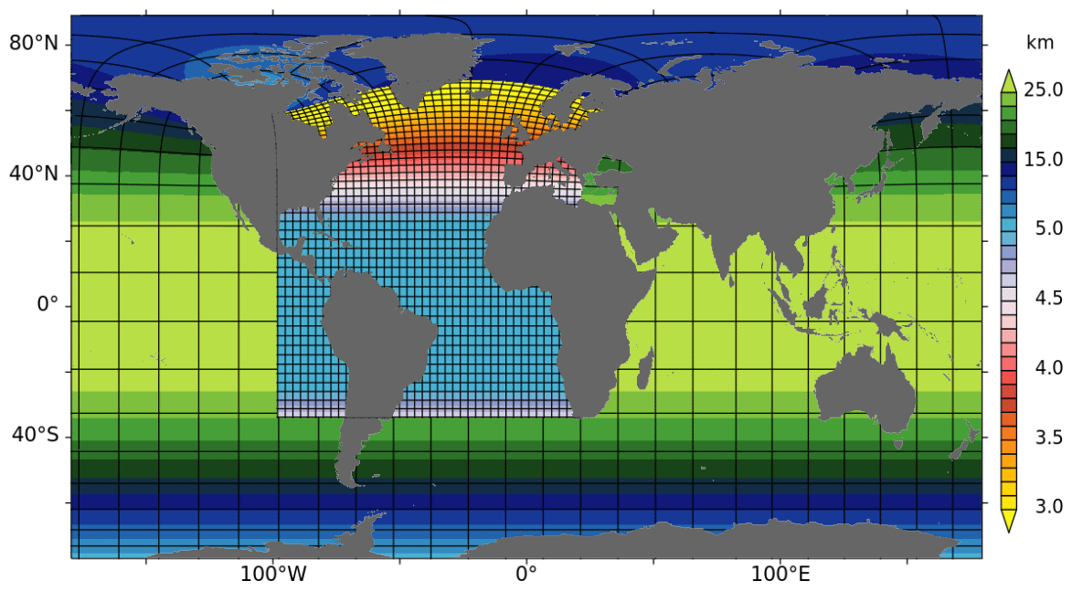
Figure 1Domain and resolution (in km) of the VIKING20X configuration. The nest area is marked by increased resolution ranging from 5 to 3 km embedded into a global ORCA025 host grid (for both grids every 60th grid line is shown in x and y directions). In total, the horizontal grid of VIKING20X consists of 1442 × 1021 cells on the host grid plus 2404 × 2499 cells on the nest grid.
2.1 ORCA025 and VIKING20X
The model simulations described and analysed in this study are based on the “Nucleus for European Modelling of the Ocean” (NEMO, Madec, 2016) code version 3.6, also involving the “Louvain la Neuve Ice Model” (LIM2, Fichefet and Morales Maqueda, 1997). The primitive equations describing the dynamic–thermodynamic state of the ocean are discretised on a staggered Arakawa C-type grid while the two-layer sea-ice model simulating one ice class with a viscous-plastic rheology is solved on a B-type grid. A global configuration (ORCA025) is used as an “eddy-present” stand-alone configuration and as a host for the eddy-rich configuration VIKING20X where “Adaptive Grid Refinement In Fortran” (AGRIF, Debreu et al., 2008) allows the resolution to be regionally increased by embedding a so-called nest, here covering the Atlantic Ocean.
The global ORCA025 (Barnier et al., 2006) is described by orthogonal curvilinear, quasi-isotropic, tripolar coordinates yielding at a finer horizontal resolution with higher latitudes at a nominal grid size of ∘. The vertical grid is given by 46 geopotential z levels with layer thicknesses from 6 m at the surface gradually increasing to ∼ 250 m in the deepest layers. Bottom topography is represented by partially filled cells with a minimum layer thickness of 25 m allowing for an improved representation of the bathymetry (Barnier et al., 2006) and to adequately represent flow over the dynamically relevant contours (f being the Coriolis Parameter and H the water depth). Together with a momentum advection scheme in vector form with applied Hollingsworth correction (Hollingsworth et al., 1983), conserving both energy and enstrophy (EEN, Arakawa and Hsu, 1990), this leads to a good representation of the large-scale, horizontal flow field (Barnier et al., 2006). For tracer advection, a two-step flux corrected transport, total variance dissipation scheme (TVD, Zalesak, 1979) is used, ensuring positive-definite values. Momentum diffusion is given along geopotential surfaces in a bi-Laplacian form with a viscosity of 15 × 1010 m4 s−1. Tracer diffusion is along iso-neutral surfaces in Laplacian form with an eddy diffusivity of 300 m2 s−1. Fast external gravity waves are damped by applying a filtered free surface formulation (Roullet and Madec, 2000) in a linearised form to ensure a volume conservative ocean. Horizontal sidewall boundary conditions are formulated as free-slip, which was demonstrated as an optimal choice in ORCA025 to benefit from the EEN momentum advection scheme in combination with partial cells (Penduff et al., 2007). Sensitivity tests during the development of VIKING20X confirmed that free-slip is also the preferred option at higher resolution. In contrast, the generation of West Greenland Current eddies was shown to work best with no-slip conditions (in the nest), which motivated its use in a region around Cape Desolation (Rieck et al., 2019). A quadratic bottom friction term is applied as vertical boundary condition. In the upper ocean, a turbulent kinetic energy (TKE) mixed layer model (Blanke and Delecluse, 1993) diagnoses the depth of the mixed layer and increases vertical mixing for unstable water columns. This includes the representation of deep convection in formation regions of deep and bottom waters.
VIKING20X consists of a global ORCA025 host grid and a nest covering the Atlantic Ocean from 33.5∘ S to ∼65∘ N (owing to the tripolar grid, the northernmost latitude varies, with a maximum of 69.3∘ N and a mean of 65.1∘ N) at a nominal horizontal resolution of ∘. Both grids are connected through a two-way nesting capability, using AGRIF with a grid refinement factor of 5 (Fig. 1). Due to its need to cover a rectangle of the host grid, the nest reaches into the Pacific Ocean to 100∘ W and cuts through the Mediterranean at ∼ 22∘ E. (Note that the eastern boundary ranges from 20∘ E in the south to 32∘ E in the north.) Both grids share the same vertical axis. The bottom topography in the nest is generated by interpolating ETOPO1 (Amante and Eakins, 2009) to the model grid and connected to the host via a transition zone along the nest boundaries. Not only bathymetry but also coast lines are thereby better resolved. To guarantee that all ocean grid cells in the nest are embedded into “wet” cells on the host grid, the coast lines on the host grid within the nested area are adjusted accordingly; an updated bathymetry is applied for the host. To meet the Courant–Friedrichs–Lewy (CFL) criterion, the time step for the integration on the nest grid is reduced by a factor of 3 compared to the host grid. The two-way nature of the nesting not only provides boundary conditions from the host to the nest but also communicates back the effect of resolving smaller-scale processes in the nested area to the global ocean. This is achieved by an exchange along the nest boundaries in both directions at every common time step of the host and nest integration (here, every third nest time step). Furthermore, the solution on the host grid is updated with the three-dimensional ocean state on the nest grid, usually every third host grid time step (for the freshwater budget corrected experiment, see below; this is done at every host grid time step).
Diffusion parameters are adjusted for the nest grid to meet the increased resolution. The Laplacian parameter for tracers is 60 m2 s−1 and the bi-Laplacian parameter for momentum is 6 × 10⁹ m4 s−1. To allow for a smooth transition between the host and the nest grids, a sponge layer is applied as a second-order Laplacian operator with a damping scale of 600 m2 s−1.
2.2 Atmospheric forcing
For the simulations used here, we employ two different atmospheric forcing sets developed for use in ocean models, CORE (version 2) (Large and Yeager, 2009; Griffies et al., 2009) and JRA55-do (Tsujino et al., 2020).
The CORE dataset is a merged product on a regular 2∘ grid covering the period 1948 to 2009. It builds on the NCEP/NCAR reanalysis which is corrected with observations and climatologies. Provided are zonal and meridional winds as well as air temperature and humidity 10 m above sea level, available as interannually varying fields at 6-hourly resolution throughout the entire forcing period. For the earlier phase, precipitation (at monthly resolution) and radiation (at daily resolution) are provided as climatology whereas for the later decades CORE incorporates precipitation (since 1979) and radiation (since 1984) as interannually varying fields from satellite-based measurements. Atmospheric fluxes are globally balanced on the basis of observed sea surface temperature and salinity data. A set of bulk formulations also provided by Large and Yeager (2009) connects the atmospheric forcing fields with the ocean model. The surface wind stress is formulated as relative winds, by using the difference between wind and ocean velocities for the calculation of the bulk formulae. CORE was used for a series of ocean model intercomparisons (OMIPs) (e.g. Griffies et al., 2009; Danabasoglu et al., 2014) and builds the basis for the official OMIP under CMIP6 (Griffies et al., 2016). For the simulation forced with the CORE dataset, we employ a monthly climatological field representing 99 of the major rivers and coastal runoff (Bourdallé-Badie and Treguier, 2006) to simulate freshwater input from land to the ocean.
The CORE dataset is no longer maintained and the forcing period therefore ends with the year 2009. As a successor, JRA55-do (used here is version 1.4) is meant to replace CORE as a common forcing product for ocean hindcasts and for model inter-comparison studies (Tsujino et al., 2018). JRA55-do (with “do” for “driving the ocean”) builds on the Japanese reanalysis product JRA-55 with improvements through the implementation of satellite and several other reanalysis products. All atmospheric forcing fields are available on a ∘ horizontal grid at 3-hourly temporal resolution covering the period 1958 to 2019. JRA55-do will be continuously extended into the present at least until 2023 (Hiroyuki Tsujino, personal communication, 2021). In the simulations in VIKING20X and ORCA025 presented here, the same bulk formulations as used in CORE are applied.
Along with the atmospheric fields, JRA55-do also provides an interannually varying daily river runoff field at ∘ horizontal resolution, which includes freshwater fluxes from ice sheets. For Greenland, this even includes the enhanced observed melting of the past decades (Bamber et al., 2018). This runoff field needs to be remapped from the JRA55-do to the ocean model grid. Here, the challenge is in the discrete placement of runoff along the different coastlines. The JRA55-do runoff covers a broader band along the coast while fjords and bays are represented differently on the two ocean model grids. The discontinuous nature of the runoff field prohibits a simple interpolation scheme. We thus created a remapping tool (https://oceanrep.geomar.de/53895/, last access: 27 August 2021) to reassign runoff to the model coastline preserving the spatial fine-scale heterogeneity of the forcing field. The runoff of each source grid node is conservatively redistributed within a radius of 55 km (80 km for VIKING20X-JRA-OMIP and ORCA025-JRA-OMIP; see next section and Table 1 for experiments) onto ocean nodes on the global (host) grid using a distance-weighted (D−3) scheme to reduce spatial smoothing of the freshwater flux. A few forcing field nodes are located farther than 55 km from the model coastline, for instance far inside fjords not represented in the model's topography. We account for this error by proportional upscaling of the remapped global runoff field at each time instance. The rather exact remapping yields some high-runoff locations, such as the Amazon river mouth with a long-term average discharge of 0.28 kg m−2 s−1. Runoff in VIKING20X-JRA-short and in VIKING20X-JRA-long before 1980 was applied including these locally very confined and high values, leading to some rare and only short-lived instabilities. To overcome these, we apply a simple river plume scheme, i.e. a spreading of the runoff within a radius of 100 km, again applying distance-based (D−1) weights to keep the focus on the actual river mouth for grid cells with at least 0.005 kg m−2 s−1 runoff, representing the 27 largest rivers in VIKING20X-JRA-long from 1980 onwards and in all other JRA55-do forced experiments. Compared to the previous runoff field used in conjunction with the CORE forcing these river plumes are considerably smaller. Runoff in the VIKING20X nest is then based on the runoff field on the host grid and interpolated onto the nest following the same procedure (Lemarié, 2006) as for all other initialisation fields. Inherent to this procedure is a spatial smoothing over 5 × 5 grid cells depending on the nesting scheme: runoff in the nest is supposed to enter the ocean in the same geographic area as it does on the underlying host grid, which has a resolution that is 5 times coarser. Note that the interpolation scheme erroneously assigns runoff to land grid cells, which we corrected by redistributing the runoff to ocean nodes within the associated 5 × 5 grid boxes.
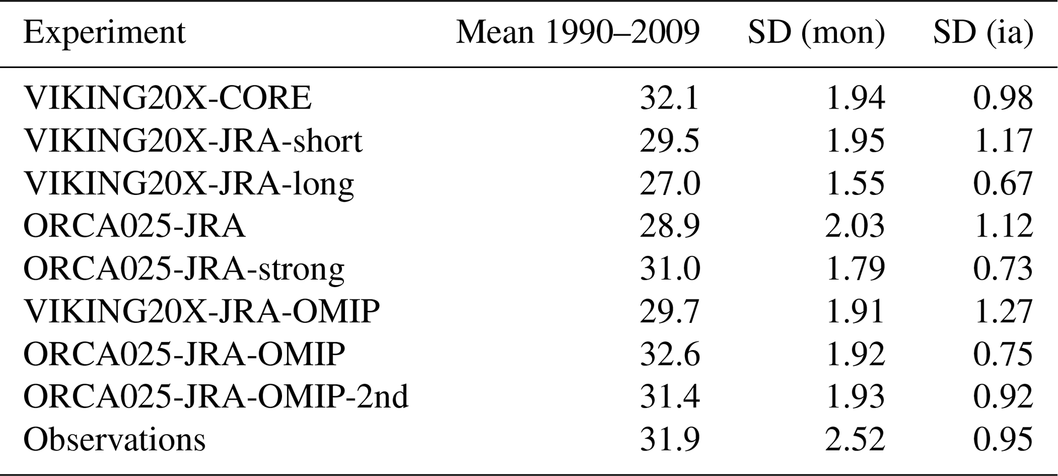
Table 1Experiments with forcing and integration period. Also provided are internal names used to identify the specific experiments. For the initialisation, “Spin-up” refers to an experiment covering the period 1980 to 2009 under CORE forcing, “Rest” to an initialisation with temperatures and salinities of WOA13 and velocities at rest. VIKING20X-JRA-short was restarted from the end state of year 1979 of VIKING20X-CORE. SSSR is the sea surface salinity restoring timescale in m yr−1; FWB is a potentially used freshwater budget correction. Experiments are grouped according to their initialisation and application of freshwater fluxes.
2.3 Experiments
A series of simulations is used in this study (Table 1). VIKING20X-CORE is an experiment forced by the CORE dataset for the period 1958 to 2009, already used and described by Rieck et al. (2019) and Hirschi et al. (2020). It is based on a spin-up integration under the interannually varying CORE forcing for the period 1980 to 2009 that originally started at rest from hydrographic conditions as provided by the World Ocean Atlas 1998 (Levitus et al., 1998) with corrections for the polar regions (PHC2.1, Steele et al., 2001). The sea-ice fields for the spin-up are initialised from a pre-spun state of a former simulation in ORCA025 to allow for a smooth start of the spin-up integration avoiding strong shocks to the fresh water budget.
Three hindcasts in VIKING20X are forced by the JRA55-do forcing: VIKING20X-JRA-short is a short hindcast integration, branched off VIKING20X-CORE at the end of 1979 and performed from 1980 to 2019 (also used in Hirschi et al., 2020). VIKING20X-JRA-long is based on the spin-up for VIKING20X-CORE and performed over the whole forcing period 1958 to 2019. VIKING20X-JRA-OMIP instead follows the OMIP-2 protocol (Griffies et al., 2016) and started from rest and an initialisation of temperature and salinities of the World Ocean Atlas 2013 (WOA13, Locarnini et al., 2013; Zweng et al., 2013). It also differs with respect to the sea surface salinity (SSS) restoring and the balance of the freshwater budget (see below). For comparison, the two long-term experiments were accompanied by experiments in ORCA025: ORCA025-JRA and ORCA025-JRA-strong following VIKING20X-JRA-long, and ORCA025-JRA-OMIP following VIKING20X-JRA-OMIP.
To reduce model drifts due to missing feedbacks from the atmosphere, a SSS restoring towards the initial climatological field is applied in most VIKING20X experiments with a piston velocity of 50 m over 4.1 years (12.2 m yr−1). This leads to a restoring timescale of 183 d for the uppermost 6 m grid cell. In sea-ice-covered areas as well as where runoff enters the ocean, restoring is not applied. Furthermore, at the river mouths vertical mixing in the upper 10 m of the water column is enhanced. ORCA025-JRA-strong, ORCA025-JRA-OMIP and VIKING20X-JRA-OMIP instead used a stronger piston velocity of 50 m yr−1 (timescale of 44 d) and a freshwater budget correction that globally balances the freshwater fluxes to zero at any host time step. In all experiments under JRA55-do forcing restoring is also not applied in an 80 km wide band around Greenland to allow for a free spread of the enhanced fresh water input to the ocean from melting ice sheets.
For comparison, in particular to assess potential restrictions due to the location of the southern boundary in VIKING20X, a nested configuration where the refinement from to ∘ applies to the South Atlantic and western Indian Ocean is used: INALT20-JRA-long, also performed under JRA55-do forcing similar to VIKING20X-JRA-long. A full description of INALT20 is provided by Schwarzkopf et al. (2019). In contrast to VIKING20X-JRA-long, the SSS restoring in INALT20-JRA-long is stronger (50 m yr−1), and the restoring also applies around Greenland. INALT20-JRA-long is initialised with the ocean state of a spin-up integration in INALT20 under CORE forcing from 1980–2009. The lateral boundary condition in INALT20-JRA-long is no-slip in the nest and free-slip on the host grid without any special treatment at Cape Desolation. Furthermore, INALT20-JRA-long includes the simulation of tides. Owing to the differences in the numerical setting, we limit the comparison to the influence of the Agulhas Current system and the Malvinas confluence region on the mesoscale and interannual variability. Both are represented in VIKING20X only on the coarser host grid but are part of the nested high-resolution region in INALT20.
It is important to acknowledge that the integration history of eddy-rich models is often less systematic than one would like to have for a consistent evaluation, often aiming at the “best” experiment under demanding computational costs. The use of accompanying experiments with ORCA025 helps to isolate individual choices, such as the SSS restoring parameter, by comparing ORCA025-JRA and ORCA025-JRA-strong. The latest experiment (VIKING20X-JRA-OMIP), also differing in the initialisation, is following Tsujino et al. (2020) and was completed during the writing of this paper. ORCA025-JRA-OMIP was already performed over a subsequently following second cycle through the JRA55-do forcing.
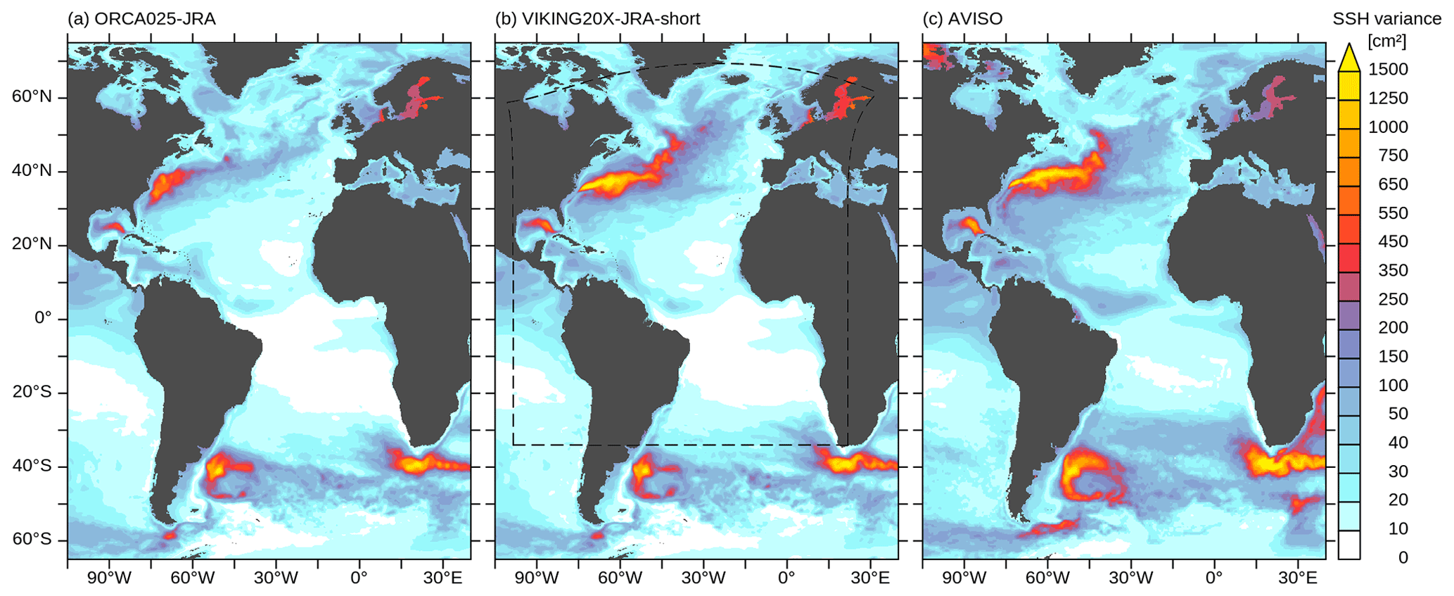
Figure 2Variance of sea surface height (in cm2) in (a) ORCA025-JRA, (b) VIKING20X-JRA-short and (c) satellite altimetry, calculated based on 5 d averages over the period 1993–2019.
We start the analyses with an evaluation of the basin-scale circulation. In contrast to the horizontal circulation, for which satellite altimetry provides a good estimate, there is no ground truth for the general structure of the AMOC. Utilising the longest available observational time series by the RAPID Programme for an evaluation of the AMOC strength and evolution, we compare the different evolution of the experiments.
The broad patterns of the mean sea surface height (SSH) are similar in all experiments (Fig. A1), reflecting a robust representation of the upper-layer circulation in the subtropical and subpolar gyres, the equatorial circulation, and the South Atlantic–Indian Ocean supergyre. For the path of the North Atlantic Current and the separation of the subtropical and subpolar gyres, VIKING20X shows a major improvement compared to ORCA025. The impact of resolution becomes even more apparent in the patterns of the SSH variability (Fig. 2). Gauged by the observational account provided by AVISO, the VIKING20X experiments show a much improved solution compared to ORCA025, applying both to the magnitude and to the horizontal patterns of the mesoscale variability at the western boundary and along open-ocean currents such as the Azores Current around 35∘ N. Prominent differences particularly concern the more realistic separation of the Gulf Stream near Cape Hatteras and the course of the North Atlantic Current in its northward turn into the Northwest Corner in VIKING20X compared to ORCA025. The latter also represents an improvement to its precursor version (VIKING20) that simulated a Northwest Corner extending too far north into the southern Labrador Sea (Breckenfelder et al., 2017).
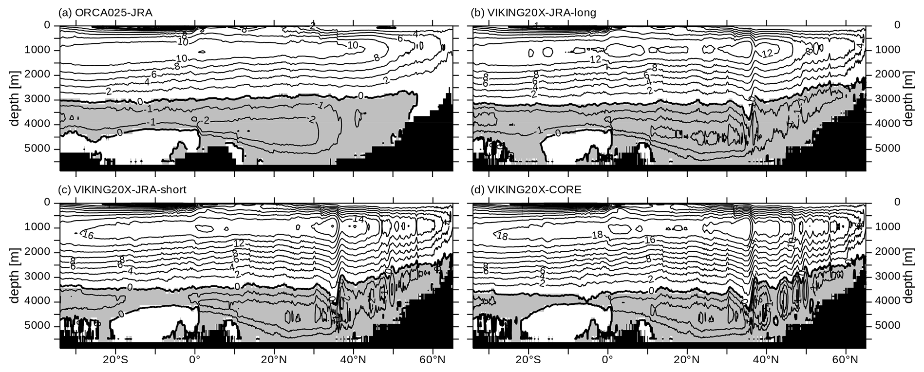
Figure 3Mean AMOC streamfunction (1990–2009, in Sv) in (a) ORCA025-JRA, (b) VIKING20X-JRA-long, (c) VIKING20X-JRA-short and (d) VIKING20X-CORE. Positive (clock-wise) contour intervals are 2 Sv, negative (counter clock-wise; grey shaded) contour intervals are 1 Sv.
Table 2Mean and standard deviation (SD) based on monthly averaged as well as interannually filtered (using a 23-month Hanning filter) data of the AMOC transport (given by the strength of the NADW cell) at 26.5∘ N. An asterisk (*) denotes a shorter averaging period (2004–2009) due to the limited length of the CORE forcing and RAPID datasets.
The horizontal circulation is largely determined by the grid resolution and the wind field. In contrast, the vertical overturning circulation depends not only on the atmospheric forcing but also on details of its application such as SSS restoring and its impact on the freshwater budget at higher latitudes (Behrens et al., 2013). The AMOC, represented by the streamfunction derived from zonally and vertically integrated meridional velocities (Fig. 3), reflects these influences in an integral way. While the general structure, with the North NADW and Antarctic Bottom Water (AABW) cells, is broadly similar in all experiments, differences are apparent in both the strength and the vertical extensions of the NADW cells. The strength of the NADW cell in ORCA025 is quite different from that in VIKING20X, with 1990–2009 average values at 26.5∘ N ranging from 10.9 to 20.4 Sv (Table 2). In the observational period (2004–2018), the JRA55-do-based experiments yield lower estimates, while VIKING20X-CORE (note the joint coverage of just 5 years) appears higher compared to observations at 26.5∘ N. Nevertheless, both VIKING20X-JRA-short and VIKING20X-JRA-OMIP fall well within the range of the observed interannual standard deviations. There is a clear resolution effect with ∼ 1–3 Sv higher transport in the ∘ simulations depending on the exact comparison (VIKING20X-JRA-long vs. ORCA025-JRA or VIKING20X-JRA-OMIP vs. ORCA025-JRA-OMIP) and time period. The NADW cell is also deeper at high resolution, indicating a better representation of the lower component of the NADW constituted by overflow across the Greenland–Scotland Ridge and the corresponding entrainment of ambient water (discussed in Sect. 4.1). Finally, there is dependency of the mean AMOC on initial conditions, as illustrated by the different strength of ORCA025-JRA-strong and ORCA025-JRA-OMIP and its subsequent second cycle. Experiments with a longer history tend to simulate a weaker AMOC, pointing to a spin-down effect (see below). This in particular applies to VIKING20X-JRA-short that starts from a relatively high level of VIKING20X-CORE, thus simulating (over the same time period) a 3–4 Sv higher AMOC compared to VIKING20X-JRA-long under the same numerical conditions.
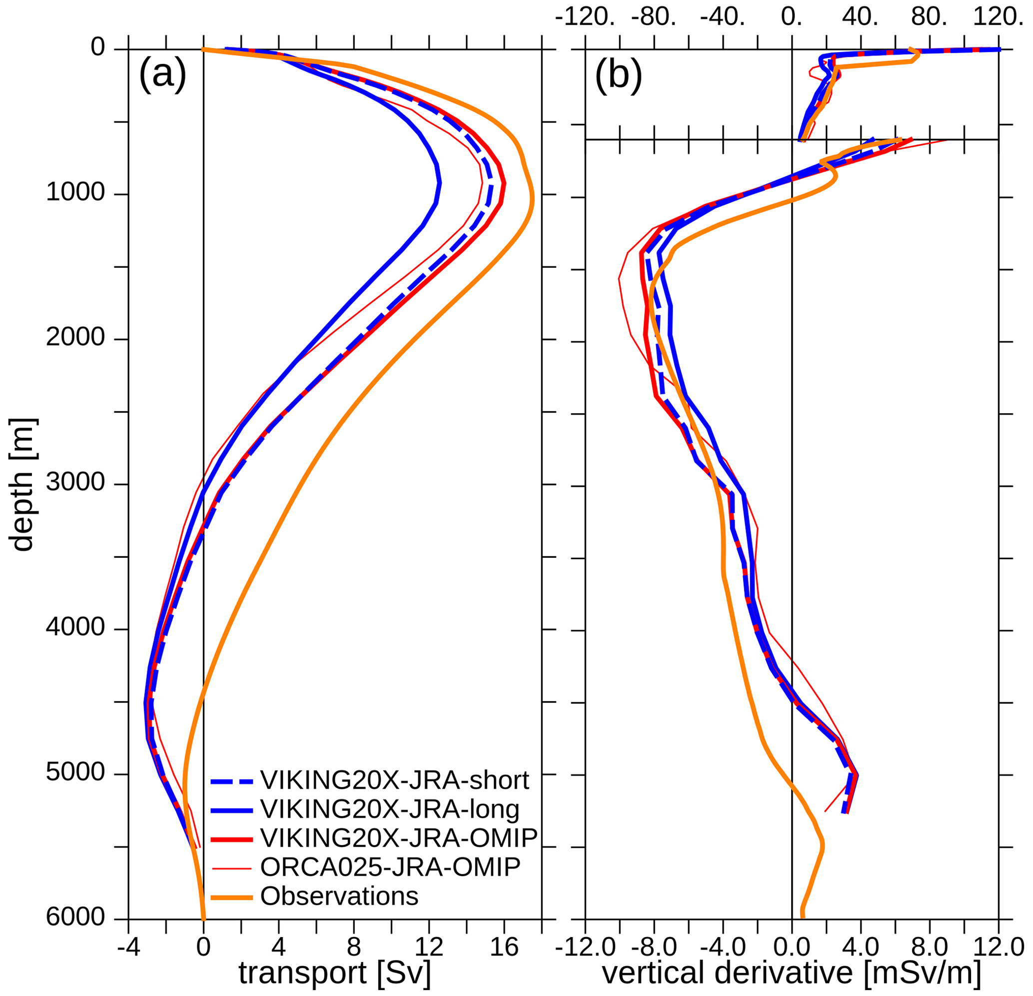
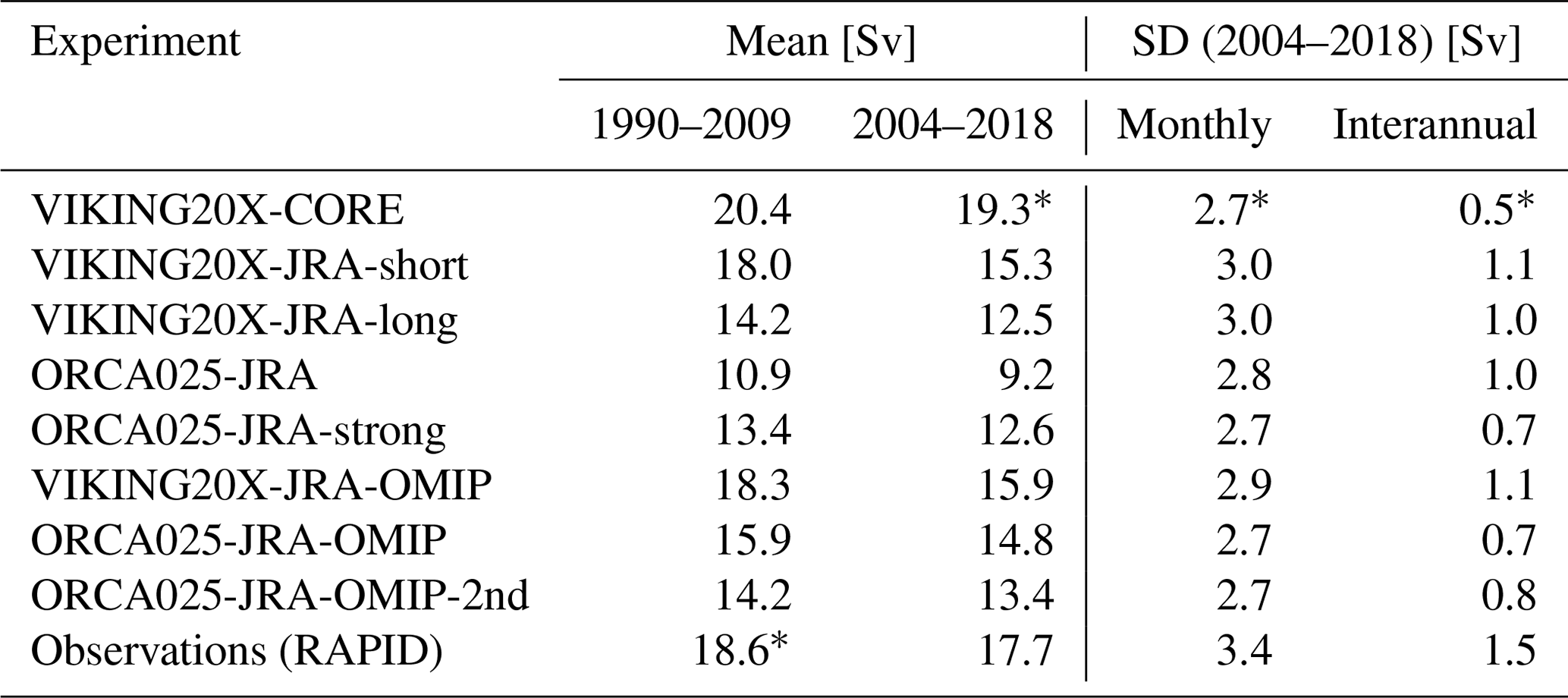
Figure 4Profiles of the (a) AMOC (in Sv) and (b) its vertical derivative (in mSv m−1) at 26.5∘ N (note the different ranges above and below 600 m depth) for experiments and RAPID observations (orange), all averaged from 2004–2018.
The RAPID data allow a more detailed evaluation of the depth structure. Figure 4a shows vertical profiles of the AMOC at 26.5∘ N; its vertical derivative represents the meridional transport per unit depth, thus providing a direct account of the northward and southward branches of the AMOC (Fig. 4b). Regarding the total strength of the NADW cell, all model results are lower than the observations (see also Table 2). Closer inspection shows that the differences mostly concern the representation of the deepest portion of the southward flow, i.e. the transport of lower NADW below ∼ 3200 m, whereas the upper part (1000–3000 m) appears reasonably well represented. The deficit in the range of lower NADW has been recognised as a long-standing, persistent issue in ocean and climate models (Fox-Kemper et al., 2019) and can largely be attributed to a loss of the high-density source waters from the Nordic Seas, e.g. by spurious mixing in the outflows across the Greenland–Scotland ridge system (Legg et al., 2006). The deficit is most pronounced in ORCA025; the representation is improved in VIKING20X, but there is still a gap by about 500 m in the reversal from southward NADW to northward AABW flow (Fig. 4b). It remains unclear if this is a result of an overly weak representation of the densest NADW, e.g. through spurious entrainment into the overflow, or by an overly strong modelled AABW cell. It could also be influenced by the choice of the reference level used for the RAPID array (Sinha et al., 2018), noting that the representation of AABW is not its major aim.
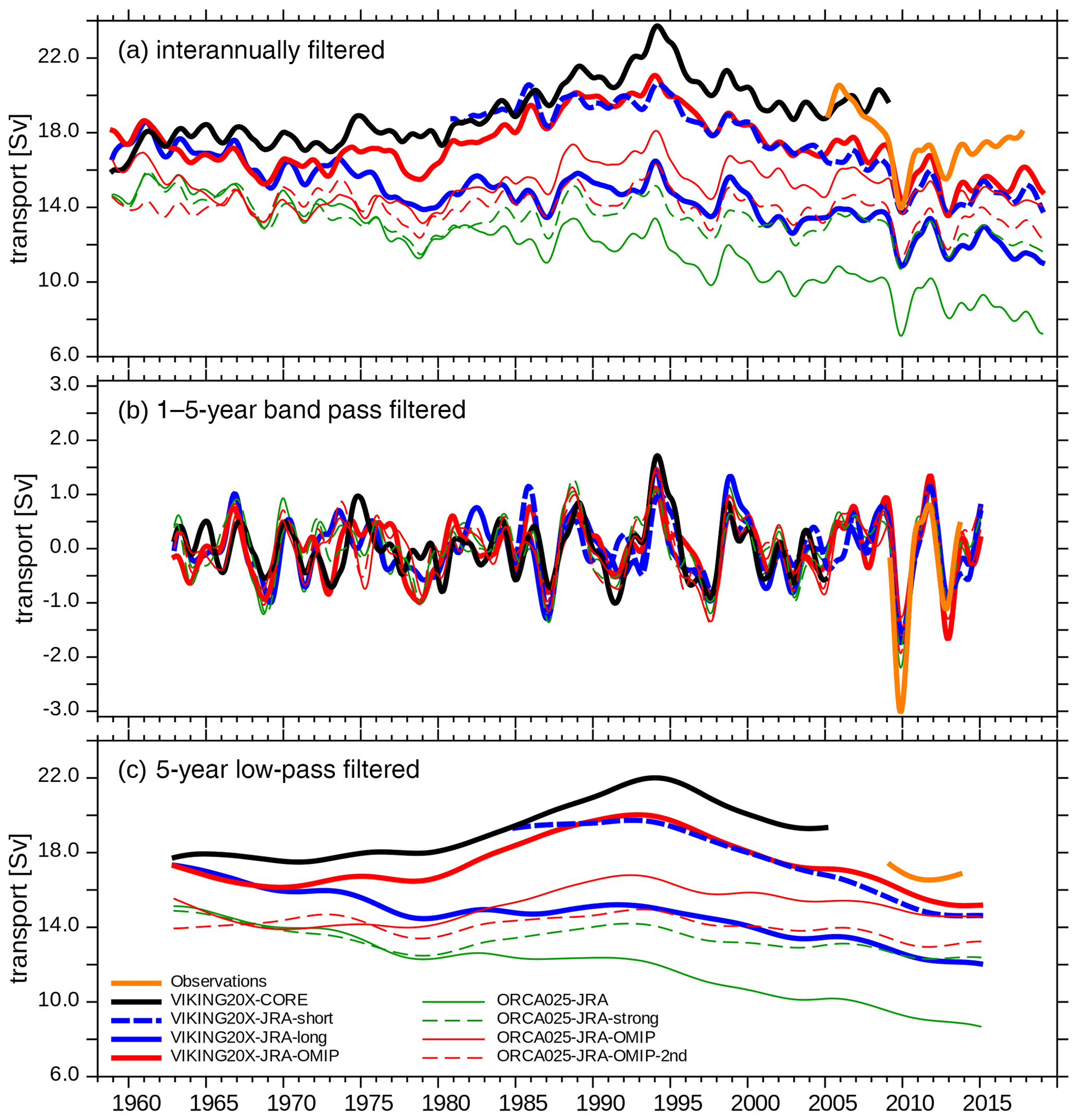
Figure 5AMOC evolution, provided by the strength of the NADW cell at 26.5∘ N: (a) full interannual, (b) 1–5-year band pass and (c) 5-year low-pass filtered time series.
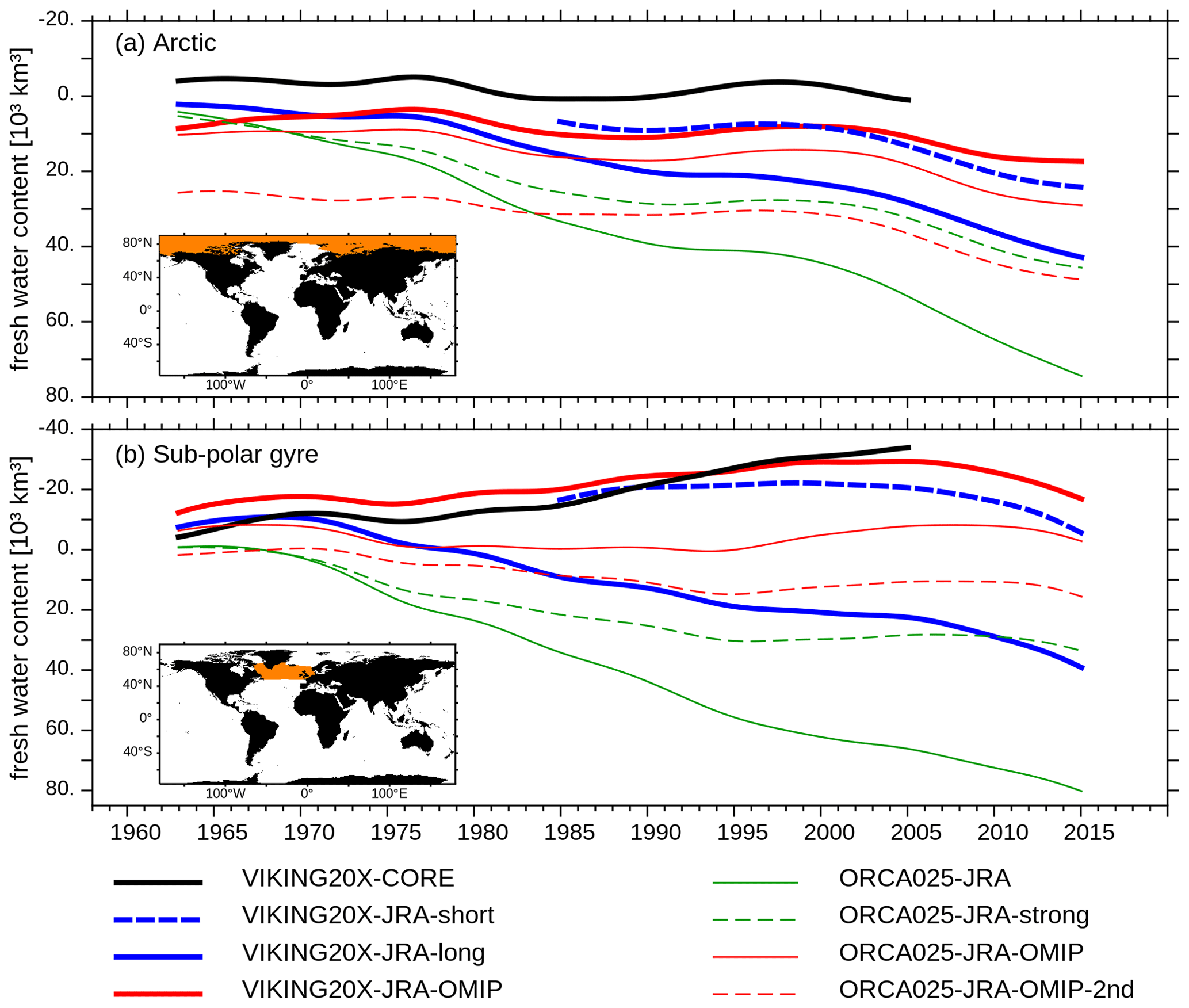
Figure 65-year low-pass filtered (a) Arctic and (b) subpolar freshwater content (computed from seawater alone, hence excluding sea-ice and snow volume, using a reference salinity of Sref=34.7, in 103 km3). Note the inverted y axis. Regions for the integration are shown as inlets.
Figure 5a shows that the AMOC in the various experiments not only differs in mean strength but also exhibits pronounced differences in its temporal evolution over multi-decadal timescales. The CORE-based experiment (VIKING20X-CORE) produces an increasing AMOC with a maximum in the mid-1990s, and a decline and stabilisation thereafter. This maximum corresponds well to the reported phase of strong convection in the Labrador Sea from observations (e.g. Yashayaev, 2007). While VIKING20X-JRA-long exhibits a long-term decline, VIKING20X-JRA-OMIP also simulates the maximum in the mid-1990s; however, in contrast to VIKING20X-CORE it continues to decline in the 2000s and beyond. The observational period of RAPID is only fully covered by the JRA55-do-based experiments. If we consider VIKING20X-JRA-OMIP and VIKING20X-JRA-short showing the “best” evolution, we note a weaker AMOC at the beginning of the observational time series, but a good representation of the 2010 minimum, which was described as a wind-related response in a negative North Atlantic Oscillation (NAO) winter (e.g. McCarthy et al., 2012). There is a tendency towards a recovery thereafter, though with a stabilisation at a weaker level, compared to the observations, towards the end of the time series.
The interannual AMOC variability, most prominently visible when also filtering out low-frequency variability, is remarkably robust among the range of experiments and compares well to the observations (Fig. 5b). The interannual correlations between VIKING20X-JRA-long, ORCA025-JRA and ORCA025-JRA-strong range around r=0.8–0.9 (1980–2009). VIKING20X-JRA-long correlates more weakly with VIKING20X-CORE (r=0.6–0.7), probably because of the different wind forcing. Within the overlapping period, all experiments show a good correlation with RAPID observations (r=0.73–0.86). This underlines the importance of the wind forcing as a major driver for the interannual variability of the AMOC strength (Danabasoglu et al., 2016). It is interesting to note that the observed monthly variability (indicated by the standard deviation in Table 2) is underestimated by 10 %–20 % with only little resolution dependency. However, the interannual variability of VIKING20X is higher than that of ORCA025, pointing to the importance of mesoscale variability for the interannual timescale. However, VIKING20X still underestimates the observations by more than 30 %. We also notice that the high variability of the latter may include errors from measurements and the processing of the different AMOC components from RAPID data.
An important aspect for the long-term evolution of the AMOC is freshwater fluxes provided by the atmospheric forcings and the numerical details of their application. This is demonstrated by also considering the ORCA025 sensitivity experiments: ORCA025-JRA-strong (dashed green lines in Fig. 5a, c) with stronger SSS restoring and applied freshwater budget correction shows a weaker trend in AMOC strength (at least post-1980s) compared to ORCA025-JRA (solid green lines). This is also indicated by VIKING20X-JRA-long and VIKING20X-JRA-OMIP (thick solid blue and red lines in Fig. 5a, c), although an initialisation effect with one experiment starting from a spin-up integration, and the other from rest, could also play an additional role here.
The long-term evolution, stable and upward in VIKING20X-CORE and downward in the JRA55-do-based experiments (Fig. 5c), can be understood through the inspection of the evolution of the freshwater content (FWC). Arctic FWC over the last couple of decades is stable in VIKING20X-CORE and VIKING20X-JRA-OMIP and increasing in the other JRA55-do-forced experiments (Fig. 6a – note the reversed y axis to match to Fig. 5c). The trend has its origin in an increased precipitation within the Arctic and sub-Arctic regions, which also causes a slight increase in the river runoff. Values of ∼ 820, 990 and 440 km3 yr−1 (VIKING20X-JRA-short, VIKING20X-JRA-long, VIKING20X-JRA-OMIP) fit into the range of observed increase of 600 ± 300 km3 yr−1 between 1992 and 2012 found by Rabe et al. (2014).
In contrast to the Arctic, the subpolar North Atlantic shows a different evolution in the JRA55-do-based experiments, depending on the application of the freshwater fluxes, and in consequence less of the forcing data itself (Fig. 6b). This effect is isolated by the two ORCA025 experiments: while ORCA025-JRA shows strong increases in FWC, the experiments with a stronger SSS restoring and freshwater budget correction, ORCA025-JRA-strong and ORCA025-JRA-OMIP, stabilise after 1980. As a result of the inability of bulk formulae to properly feed back to the (largely prescribed) atmosphere, Griffies et al. (2009) have described a positive feedback between AMOC strength and freshwater forcing, with additional freshwater in the subpolar North Atlantic limiting deepwater formation. The corresponding reduction of the AMOC would cause less salt transported northward, in consequence leading to a further freshening of the subpolar North Atlantic (Behrens et al., 2013). Both VIKING20X-JRA-OMIP and ORCA025-JRA-OMIP seem to minimise the positive feedback between subpolar North Atlantic FWC and AMOC through stronger SSS restoring and a global freshwater budget correction, obviously lowering the FWC trend in the subpolar gyre.
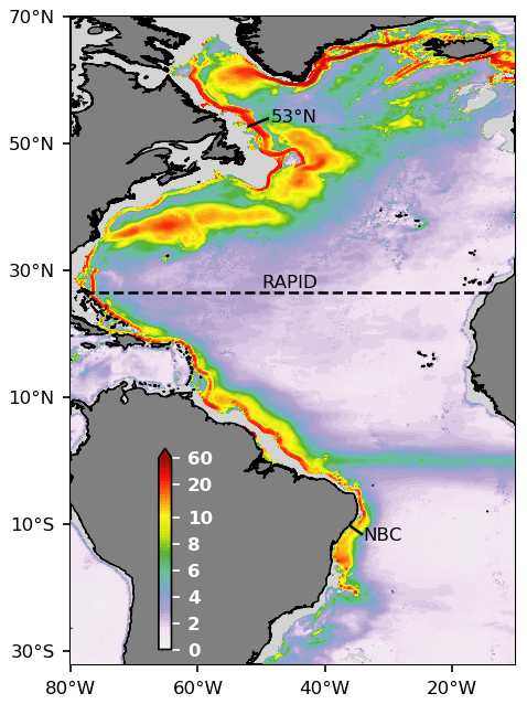
Figure 7Mean horizontal current speed (1990–2009, in cm s−1), averaged between σ0=27.65–27.95 in VIKING20X-JRA-short. Regional sections are indicated by black lines.
While a clear attribution of the AMOC trends to either physical drivers (i.e. atmospheric forcing and runoff) or spurious model drift is not possible at this stage, we can use the range of solutions with their diverging trends to assess their manifestation in regional current systems and thereby explore if and how regional observational arrays may be capable of depicting the long-term evolution and variability of the AMOC. An important part of the analysis is the formation and spreading of deepwater masses. From a number of observational and modelling studies, Lozier (2010) concluded that NADW only partly follows a coherent Deep Western Boundary Current (DWBC) as explained by classical theory (Stommel, 1958). In several parts of the Atlantic Ocean deviations into the interior, recirculations and disruptions by deep mesoscale eddies play an important role in the spreading.
Figure 7 illustrates the circulation in NADW layer, indicating the spreading from the Nordic Sea through the Denmark Strait and through the Faroe Bank Channel, the latter flowing around and crossing through gaps of the Reykjanes Ridge (Zou et al., 2017). The coherent path around Greenland is broken into mesoscale eddies in the northern Labrador Sea, reaching even down into this density range (Rieck et al., 2019), and reconfines again on the Canadian side. The export of NADW from the subpolar into the subtropical North Atlantic and further into the South Atlantic has been subject to many studies (e.g. Bower et al., 2009). General consensus, indicated by models and observations, is that a large part of NADW is deviated on a broad path towards the mid-Atlantic ridge (Lozier et al., 2013; Gary et al., 2011; Biló and Johns, 2019; Le Bras et al., 2017), with only a narrow portion of the DWBC flowing around the Flemish Cap and through the Flemish Pass. Only at around 30∘ N is the flow towards the south seen again as a coherent DWBC, but it is also subject to local recirculations (Schulzki et al., 2021). In the South Atlantic, the DWBC again breaks up into mesoscale eddies (Dengler et al., 2004) and then fades out at around 20∘ S. A zonal band of slightly elevated speed between 20 and 25∘ S indicates the flow of NADW water described by Van Sebille et al. (2012) which could also be identified in our simulations by Lagrangian experiments (not shown here).
From the evaluation in this section, we conclude that the VIKING20X configuration successfully represents the basin-wide horizontal circulation. The strength of the overturning circulation is sensitive to the atmospheric forcing and numerical choices. VIKING20X-CORE, VIKING20X-JRA-OMIP and VIKING20X-JRA-short all simulate a realistic AMOC strength (the latter two JRA55-do-based simulations include more recent years). In the following section we will explore how different AMOC evolutions are reflected in regional current systems.
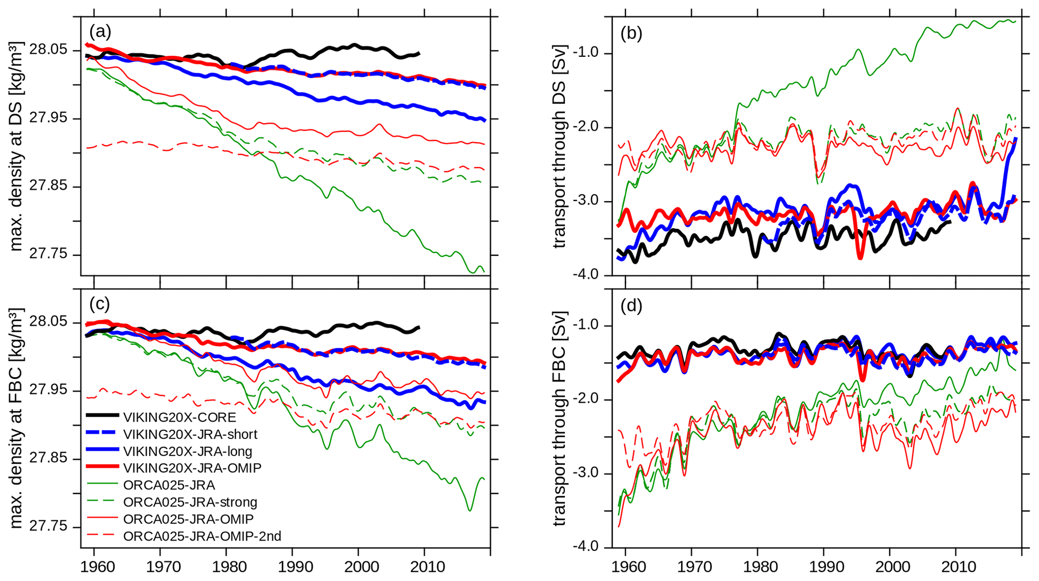
Figure 8Evolution of maximum overflow density and the overflow transport in the (a, b) Denmark Strait and the (c, d) Faroe Bank Channel. Overflow transport estimates are based on southward transport of waters with density larger than 27.70 kg m−3 below 270 m.
Table 3Maximum density and overflow transports provided as mean and monthly standard deviation for the period 1990–2009 at Denmark Strait sill and Faroe Bank Channel. Overflow transports are based on southward transport of waters with density larger than 27.70 kg m−3 below 270 m.

4.1 Subpolar North Atlantic
The subpolar North Atlantic is a key region for the AMOC (Schott and Brandt, 2007). It receives surface water masses from the subtropics and overflow water from the Nordic Seas. Here, the different components of the NADW are formed through exchange with the atmosphere and mixing processes (Marshall and Schott, 1999). They directly maintain the strength of the AMOC and modulate its variability (Böning et al., 2006).
The densest component of the NADW is formed in the Nordic Seas: through heat loss to the atmosphere and sea-ice formation, dense water is formed and, by convection, builds a large reservoir at depth between Greenland, Iceland and Norway (Dickson and Brown, 1994; Blindheim and Osterhus, 2005). It then spills over the Greenland–Scotland Ridge into the subpolar North Atlantic. Two narrow passages, the Denmark Strait between Greenland and Iceland with a sill depth of 650 m and the Faroe Bank Channel between the Faroe Islands and Scotland with a sill depth of 850 m, funnel this exchange. Figure 8 and Table 3 show density and transport through both passages. With transports of around 3 Sv and little variability through the Denmark Strait, the mean transport in VIKING20X compares well to the observational estimates (3.1 Sv by Jochumsen et al., 2017, and 3.5 Sv by Harden et al., 2016). Transports through the Faroe Bank Channel are around 1.4 Sv, thus smaller than the reported 2.2 Sv (Hansen et al., 2016; Østerhus et al., 2019; Rossby et al., 2018) to 2.7 Sv (Berx et al., 2013). ORCA025 instead simulates an enhanced transport which (in parts) can be attributed to the 40 % larger cross section at ∘ resolution compared to ∘. The simulated maximum density is typically smaller than the reported σ0=28.05–28.07 (Harden et al., 2016; Hansen et al., 2016), which can also be due to the limited vertical resolution not resolving the bottom boundary layer.
Except for a strong weakening trend in ORCA025-JRA and a spin-down in the first decades of ORCA025-JRA-OMIP, transports do not show a long-term trend and are quite stable. This is probably a result of the continuous supply of dense water north of the sills and hydraulic control limiting the transport to its given value (Käse et al., 2003). More important than the transport itself is the density of the overflow water. Previous studies described a direct link between overflow density and AMOC strength (Behrens et al., 2013; Latif et al., 2006), although the exact reason for this is still unclear and debated. For example, Danabasoglu et al. (2014) do not find such a link in the variety of CORE-based experiments. Here we do see a similar behaviour of both overflow density and AMOC, with stable densities in VIKING20X-CORE and (different) weakening trends in VIKING20X-JRA-long, VIKING20X-JRA-short and VIKING20X-JRA-OMIP. ORCA025-JRA shows a decline in overflow densities, stronger than anticipated from the AMOC trend (Fig. 5). However, similar to the AMOC, ORCA025-JRA-strong shows a weaker declining trend compared to ORCA025-JRA after 1980. In ORCA025-JRA this is also reflected in the overflow transport. It is interesting to note that the first cycle in ORCA025-JRA-OMIP shows a similar stabilisation in overflow density after about 25 years. The second cycle is subject to a lighter density which is also reflected in a weaker AMOC (Fig. 5). In contrast, VIKING20X-JRA-OMIP does not show such a spin-down in overflow density nor AMOC strength.
In the subpolar North Atlantic, further deepwater is generated and added to the NADW. Owing to strong wintertime heat loss, in particular through strong and cold winds, the Labrador and Irminger Seas are regions of deepwater formation. Deep convection provides a lighter, upper component to the NADW (in contrast to the overflows forming lower NADW).
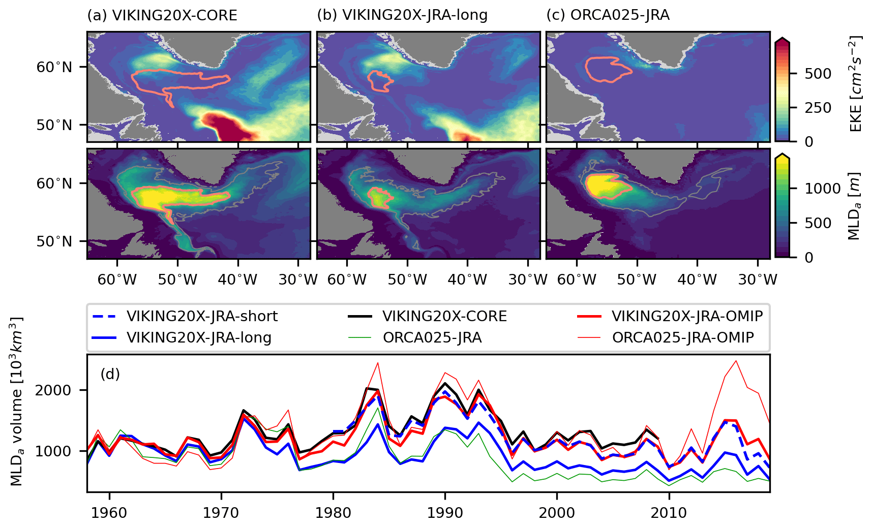
Figure 9Spatial pattern and temporal variability of mixed layer depth (MLD) (i.e. the depth that exceeds density at 10 m depth by 0.01 kg m−3) in the subpolar North Atlantic: long-term (1980–2009) mean eddy kinetic energy (EKE) at 112 m depth and annual maximum MLD (MLDa) in (a) VIKING20X-CORE, (b) VIKING20X-JRA-long and (c) ORCA025-JRA, light red contours highlight long-term mean MLDa>1000 m and grey contours the long-term maximum MLDa>1000 m; (d) interannual variability of spatially integrated MLDa, resulting in a volume.
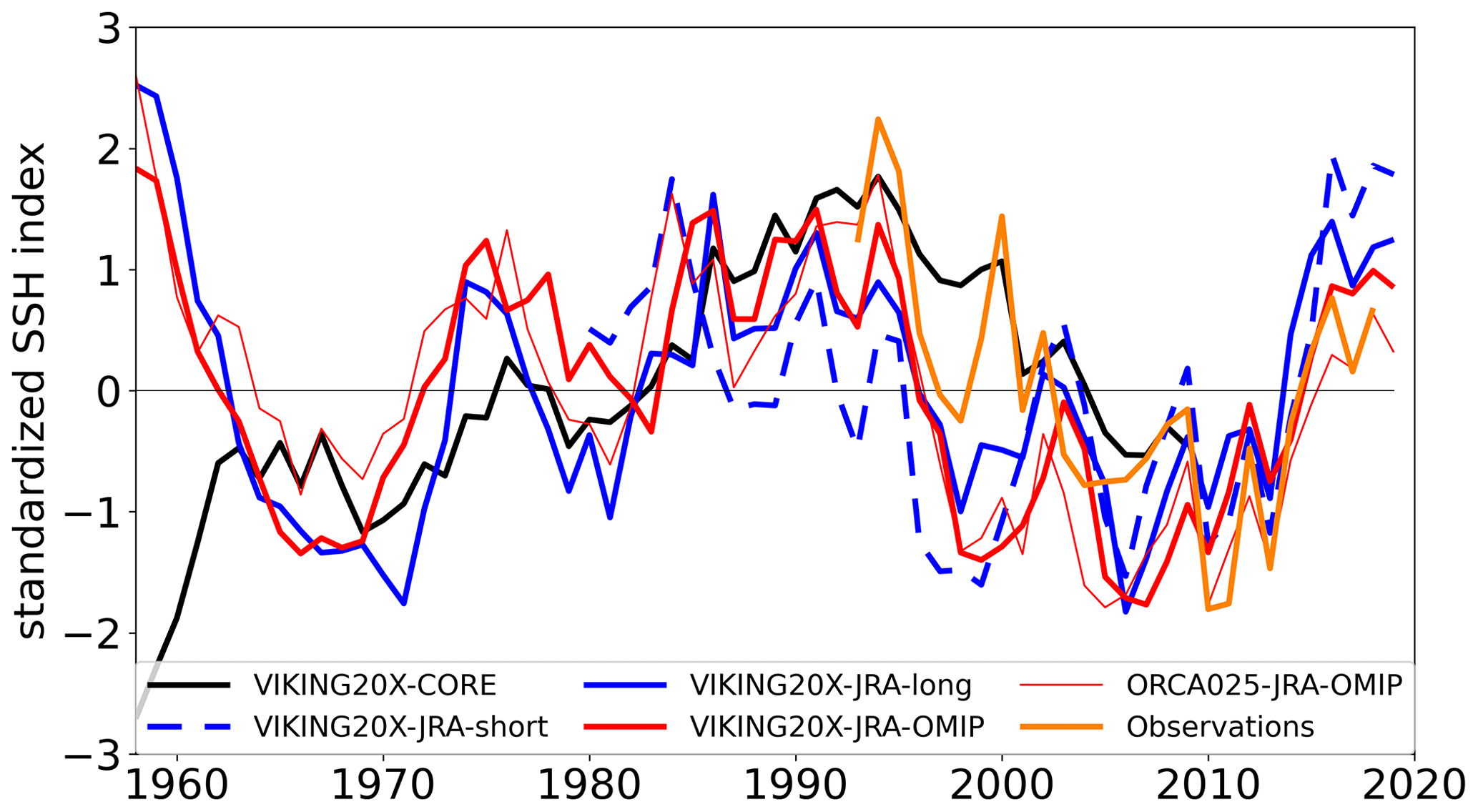
Figure 10Time series of the annual mean subpolar gyre index in the experiments and based on observations (orange). Here, the index is defined as the second principle component of an empirical orthogonal function analysis for non-detrended SSH in the North Atlantic between 20 and 70∘ N.
The distribution of long-term mean annual maximum mixed layer depth (MLDa, Fig. 9a–c) shows that the spatial patterns of deep convection are influenced by both the ocean model resolution and the atmospheric forcing. In VIKING20X simulations the centre of deep convection in the Labrador Sea, here indicated by the light red line encompassing the area where long-term mean MLDa exceeds 1000 m, is limited in the north through the impact of travelling Irminger rings visible through a tongue of elevated eddy kinetic energy (EKE) (Fig. 9a–b; note that the pattern for VIKING20X-JRA-short and VIKING20X-JRA-OMIP are not shown but are very similar to VIKING20X-CORE) as thoroughly described by Rieck et al. (2019). As Irminger rings are not properly represented in ORCA025, the centre of deep convection here extends further to the northwest (Fig. 9c). Moreover, in all model simulations, the potential deep convection region, here indicated by the light grey line encompassing the area where long-term maximum MLDa exceeds 1000 m, extends into the Irminger Sea. However, the area covered by the centre of deep convection as well as by the potential deep convection region vary among the different model simulations, with no clear relation to the model resolution. While there are little differences between VIKING20X-CORE, VIKING20X-JRA-short and VIKING20X-JRA-OMIP (not shown), VIKING20X-JRA-long and ORCA025-JRA feature overall smaller areas and ORCA025-JRA-OMIP (not shown) larger areas than the first three mentioned experiments.
While the resolution seems to determine the general spatial structure, the forcing and other model-specific settings impact the intensity and temporal variability of deep convection. During the first 15 years, i.e. until the mid-1970s, the MLDa volume in the depicted domain (Fig. 9d) shows nearly the same magnitude and temporal variability for all simulations (notably, the overall mixed layer volume in the ORCA025 simulations is not systematically larger than in the VIKING20X simulations). Afterwards, MLDa volume and variability in VIKING20X-JRA-long and ORCA025-JRA decrease compared to the other simulations. The smaller MLDa volume is a result of shallower MLDa over the whole domain, including reduced convection intensity in the central deep convection areas. A causal relation between MLDa and AMOC is subject to discussion in the light of the recent observational findings by Lozier et al. (2019) and a topic not thoroughly addressed here, but one deserving further study. Here we note that in VIKING20X-JRA-long and ORCA025-JRA the decrease in MLDa volume sets in after the simulated AMOC decline described above. At least parts of the diagnosed negative MLDa volume trends in VIKING20X-JRA-long and ORCA025-JRA can be attributed to spurious model drifts.
Table 4Correlations of the annual mean gyre index with observations for the period 1993–2009. Correlations are significant at 99 %, except the one for VIKING20X-JRA-short (80 %).
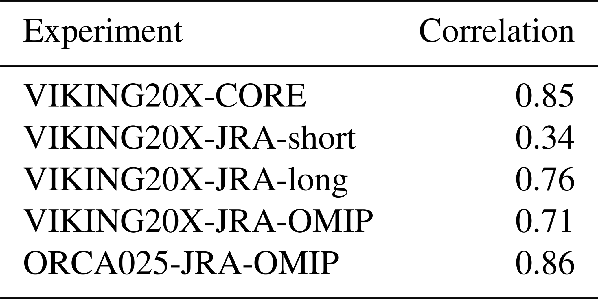
Table 5DWBC export (mean and standard deviation) across 53∘ N for different periods, characterised by the NADW defined by σ2 criteria (ORCA025-JRA >36.52, ORCA025-JRA-strong >36.63, VIKING20X-JRA-long >36.59, VIKING20X-JRA-short >36.68, VIKING20X-CORE >36.72, ORCA025-JRA-OMIP >36.73 and VIKING20X-JRA-OMIP >36.69), and 20-year trends.
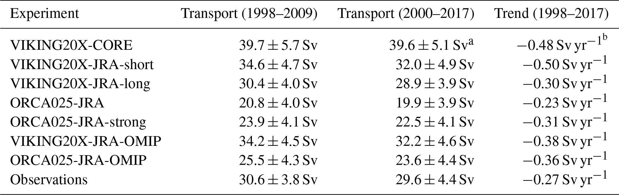
a 2000–2009. b 1998–2009.
In comparison to observations the MLDa patterns in the VIKING20X simulations (including the occasionally large MLDs in the Irminger Sea) seem more realistic than that of other model simulations at lower or comparable resolution. Moreover, the temporal evolution of the mixed layer volume in VIKING20X-CORE, VIKING20X-JRA-short and VIKING20X-JRA-OMIP agrees very well with the reported history of deep convection in the subpolar North Atlantic (while VIKING20X-JRA-long and ORCA025-JRA seem to miss a clear maximum of mixed layer volume and deep convection intensity in the 1990s, and ORCA025-JRA-OMIP experiences an overly strong intensification of deep convection in recent years). A more detailed evaluation and interpretation is presented by Rühs et al. (2021).
The circulation in the subpolar North Atlantic can be characterised by an index based on sea surface height. Following Koul et al. (2020), the subpolar gyre index is defined as the second principle component of empirical orthogonal function (EOF) analysis with non-detrended data. It is highly correlated steric sea-level changes, i.e. upper ocean density variations in the gyre centre, which are largely connected to changes in the NAO index and impact the upper ocean salinity in the eastern subpolar North Atlantic. A density increase in the centre intensifies the gyre through geostrophic balance (both a stronger and larger gyre, index >0), reduces the throughput of subtropical waters and hence leads to a freshening of the eastern subpolar North Atlantic.
Figure 10 shows that the annual mean subpolar gyre index of most experiments is correlated with observations (Table 4). The experiments also seem robust on longer, decadal timescales, with a strong subpolar gyre in the 1990s, a weakening thereafter and a recovery in the mid-2010s. Both maxima are reflected in the convection strength (the second one at least in VIKING20X-JRA-short, VIKING20X-JRA-OMIP and ORCA025-JRA-OMIP; see Fig. 9).
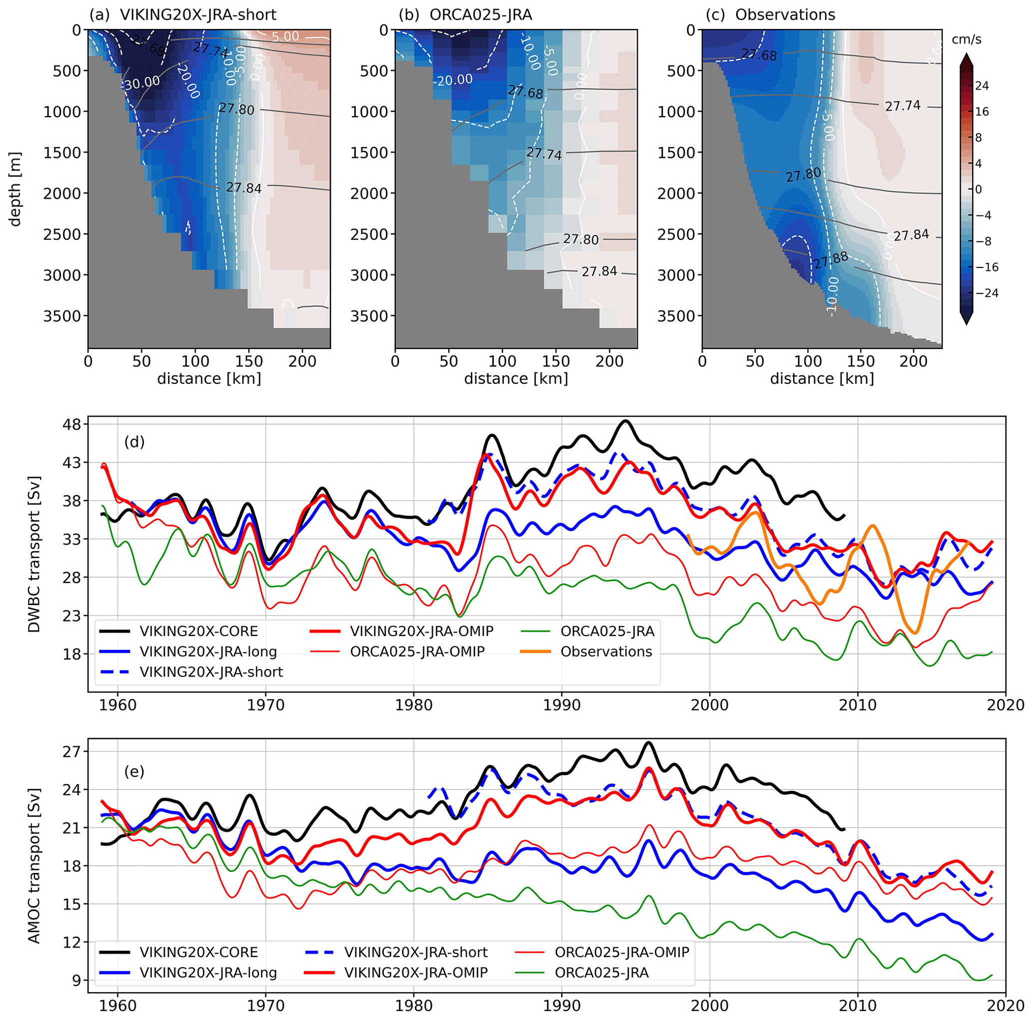
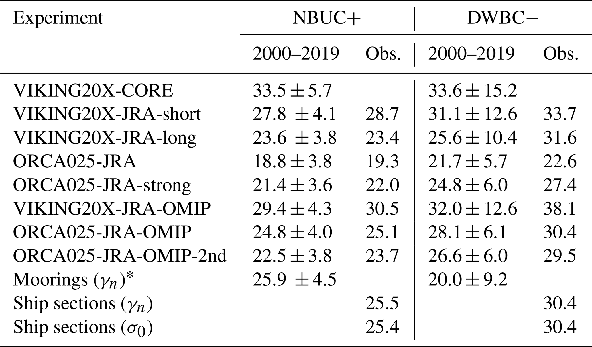
Figure 11Mean sections (a, b, c) of velocity and σ0 isolines (1997–2009) at 53∘ N in (a) VIKING20X-JRA-short, (b) ORCA025-JRA and (c) observations (non-linear colour map is used with intervals given of 1 Sv between −8 and 8 Sv, and 2 Sv beyond that range). Time series of (d) the DWBC export across 53∘ N characterised by the NADW defined by σ2 criteria (Table 5), following the analysis of Handmann et al. (2018) and (e) the AMOC transport in σ2 density coordinates at 53∘ N.
One important key location picking up the different constituents and timescales of subpolar gyre variability and deepwater formation is the observational array off Labrador at 53∘ N (Zantopp et al., 2017). The DWBC at this location is seen as an index for the subpolar AMOC and for the overall AMOC on decadal and longer timescales due to the increasing meridional coherence (Böning et al., 2006; Bingham et al., 2007; Wunsch and Heimbach, 2013; Buckley and Marshall, 2016, see also discussion). Since 1997 this mooring array has recorded all three constituents of the NADW exiting the Labrador Sea via the DWBC (Zantopp et al., 2017; Fischer et al., 2004). The observations revealed a 100–150 km wide well-defined cyclonic (southward) boundary current, featuring a strong barotropic component with significant baroclinic flow in the shallow velocity maximum of the Labrador Current and the deep velocity maximum (typically 0.25 m s−1, reaching up to 0.4 m s−1) associated with the lower NADW, and an anticyclonic recirculation in the interior Labrador Sea (Fischer et al., 2004; Lavender et al., 2000). Figure 11a–c show that the general structure of the narrow boundary current system is visible especially in VIKING20X. Similarly to experiments with the predecessor VIKING20, they produce a stronger surface maximum, a weaker deep velocity maximum and a stronger recirculation than in observations (Handmann et al., 2018). In the ORCA025 experiments the boundary current appears too wide with a split surface maximum and no deep boundary current core, the latter pointing to an overly strong erosion of lower NADW on its way around the Irminger and Labrador Seas. Both ORCA025-JRA and VIKING20X-JRA-short are more barotropic than found in observations, though one finds a clear improvement of the representation of the spatial scales and location of the DWBC at 53∘ N in VIKING20X-JRA-short. The density structures (grey lines in Fig. 11a–c) reveal a discrepancy between the models and observations. VIKING20X compares better to the observations than ORCA025, which is the effect of a combination of a denser overflow (Table 3) and a better representation of the downslope flow and its associated entrainment of ambient water masses. For the comparison of NADW transports at 53∘ N the water mass boundary between the upper AMOC component and the NADW was adjusted for each individual model using the mean density of the AMOC maximum at the OSNAP section over the full model integration (Handmann et al., 2018). Owing to the improved representation of lower NADW, the VIKING20X experiments simulate NADW transports that fall into the observed standard deviation (Table 5). With respect to the longer-term temporal variability (Fig. 11d), it is apparent that the observations feature stronger multi-annual variability than the model experiments. There is no significant correlation between the simulations and the observed transports on interannual timescales (here not shown). However, both observations and model experiments show a significant downward trend that is usually stronger in most of the simulations (Table 5). The general temporal evolution, though subject to much less variability on multi-annual timescales, reflects that of the AMOC (Fig. 11e). It is important to note that the AMOC in depth coordinates is of little use in the subpolar North Atlantic. In contrast to the lower latitudes, the “overturning” is not given by an upper–warm and deeper–cold contrast but rather a strong east–west gradient responsible for the transport across density surfaces (Danabasoglu et al., 2014; Biastoch et al., 2008a).
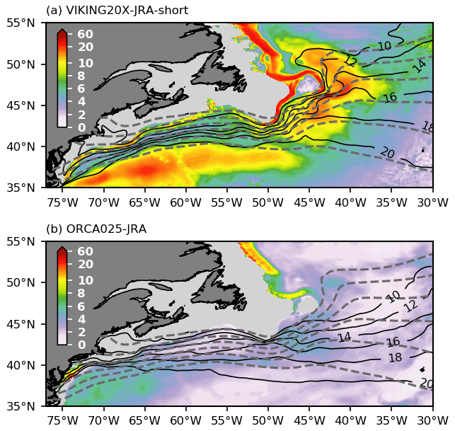
Figure 12Path of the DWBC (speed on density range; see Fig. 7) and SST in degrees Celsius (solid contours) for (a) VIKING20X-JRA-short and (b) ORCA025-JRA. SST from the HadiSST dataset (Rayner et al., 2003) is shown by dashed contours.
Table 6Mean and standard deviation (SD) based on monthly (mon) averaged as well as interannually (ia) filtered data of the transport (in Sv) through Florida Strait for the period 1990–2009. In this period, data coverage from cable measurements is 82 %.
4.2 Subtropical North Atlantic
Current structures associated with the export of deep water masses from the subpolar into the subtropical North Atlantic follow interior pathways and only a specific narrow DWBC (Fig. 7). This is in particular visible around the Flemish Cap and through the Flemish Pass (Fig. 12). While completely absent in ORCA025, VIKING20X shows a continuous path around the Flemish Cap, followed by a narrow and weak current along the American shelf. Solodoch et al. (2020) noticed the strong fluctuations in the DWBC at the Flemish Cap due to steep bathymetric variations. This is not necessarily an eddying signal but could also be caused by topographic Rossby waves related to Gulf Stream rings and meanders (Peña-Molino et al., 2012). Details of the deep pathways seem to be connected to the overlying flowing Gulf Stream, so that its correct separation at Cape Hatteras and path into the Northwest Corner might play an important role. Horizontal resolution is also of relevance here: Chassignet and Xu (2017) noticed a much more realistic separation and path of the Gulf Stream if simulated at ∘ compared to ∘. However, they also noted that ∘ is required to fully represent the Gulf Stream penetration and the associated recirculation gyres at depth. Nevertheless, Fig. 12 shows that the separation of the Gulf Stream and the swing into a Northwest Corner is already well reproduced in VIKING20X as indicated by the sea surface temperature (SST) distribution. In contrast, ORCA025-JRA features the overly zonal path of the North Atlantic Current common for lower-resolution models. This is a typical behaviour even at ∘ resolution as demonstrated by Chassignet and Xu (2017).
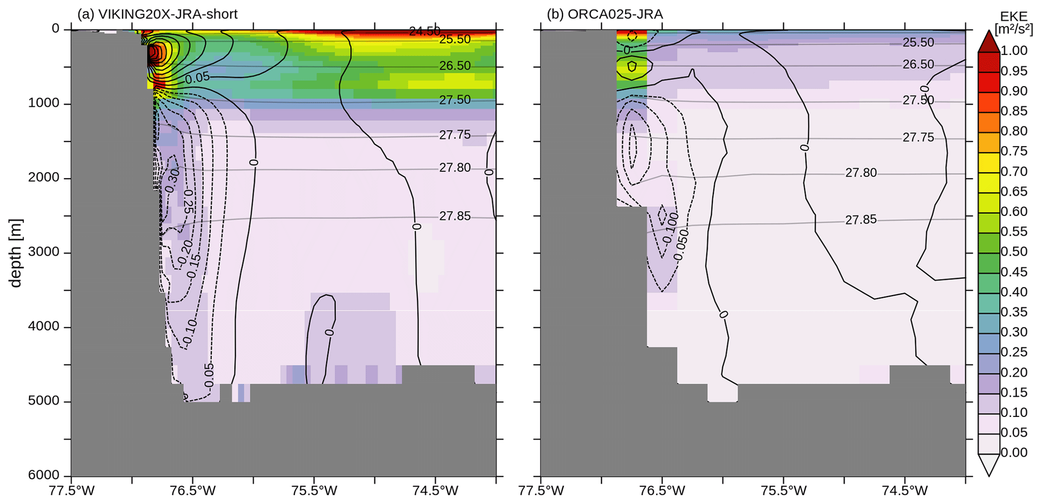
Figure 13Mean (1990–2009) eddy kinetic energy (EKE) in m2 s−2 (shaded) and meridional velocity in m s−1 (black contours) section at 26.5∘ N for (a) VIKING20X-JRA-short and (b) ORCA025-JRA with σ0 isolines (grey). The Antilles Current is depicted by positive, northward velocities above 1000 m depth near the coast.
In the subtropical North Atlantic, the southward flow of NADW is again concentrated along the western boundary (Fig. 7). It aligns with the northward-flowing surface branch of the Antilles Current (Fig. 13), which is complemented by the flow through the Florida Strait. The characteristics of the AMOC introduced in the subpolar and subarctic regions, but also details of the bathymetry south of it, have an imprint in the current structure at the western boundary. In ORCA025 the flow of NADW clearly lacks the denser part of the NADW because of the inability to maintain the overflow at this resolution, while in VIKING20X the DWBC reaches much deeper. This is also reflected in the integral measures of the AMOC (Figs. 3 and 4). The surface branch instead depends on the representation of the Bahamas Islands and the Bahamas Bank. In VIKING20X the Antilles Current is variable, and eddies are crossing the section at 26.5∘ N northwestward, providing a prolonged maximum of EKE (Fig. 13a). ORCA025 has a much weaker and stable surface transport, with even southward transport directly at the surface.
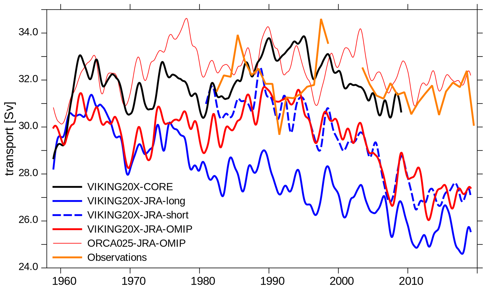
Figure 14Time series of the transport through Florida Strait from experiments (interannually filtered) and from cable measurements (orange) given as yearly averages for years with data coverage >70 %.
An important component of the RAPID observational array (and motivation for the choice of its particular latitude) is the long-term measurements of the transport through the Florida Strait obtained from voltage differences with telephone cables (e.g. Meinen et al., 2010) as shown in Fig. 14. Table 6 demonstrates that the Florida Current transports agree well with the observations within 1-2.6 Sv for VIKING20X-CORE, VIKING20X-JRA-short and VIKING20X-JRA-OMIP. The transport is weaker in VIKING20X-JRA-long, which could correspond to the lower AMOC. Since wind forcing is similar in VIKING20X-JRA-short and VIKING20X-JRA-long, this difference can be attributed to the thermohaline part of the Florida Current. Variability of the Florida Current transport in all model simulations is underrepresented at monthly timescales, but comparable to observations at interannual timescales. In contrast to the pure metric (Table 6), we find a wide range of temporal variability. Some of the JRA55-do experiments are correlated on interannual timescales, but none of the experiments is correlated with the observations (Fig. 14). Also, some experiments (e.g. VIKING20X-CORE and VIKING20X-JRA-OMIP) showed a correlation of ∼ 0.75 between the Florida Current and the AMOC, while others (in particular VIKING20X-JRA-long, but also the experiments in ORCA025) did not. This demonstrates that the Florida Current is not just a WBC closure in the form of net (wind-related) Sverdrup changes from the interior but is rather regionally influenced from the flow through the Caribbean Sea and through regional atmospheric forcing (Lee and Williams, 1988; DiNezio et al., 2009; Hirschi et al., 2019).
Surprisingly, all VIKING20X experiments (including VIKING20X-CORE) show a declining trend that starts in the 1990s which is not reflected in the latter part of the observations. The VIKING20X experiments forced by JRA55-do simulated a decline of the Florida Current of ∼ 0.1 Sv per year over the RAPID period 2004–2018, which is about 27 %–43 % of the AMOC in the same period (here not shown).
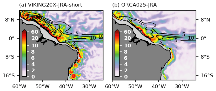
Figure 15Snapshot of the path of the DWBC speed (5 d mean centred around 22 February 1990, density range as in Fig. 7) and upper-ocean eddy kinetic energy (contours, in J m−3, mean between 1990–2009 for the upper 1000 m) for (a) VIKING20X-JRA-short and (b) ORCA025-JRA.
Table 7Mean and monthly standard deviation of NBUC and DWBC transports across 11∘ S from 12 observational sections, mooring measurements and experiments for the period 2000–2019 (for VIKING20X-CORE 2000–2009) and sampled from monthly data according to the ship-based observational coverage (Obs.). The transport calculation is modified from Hummels et al. (2015) by changing from γn to almost equivalent σ0 criteria. For observations, transports based on γn criteria are given as reference. (NBUC transport is calculated by integration of positive velocities in three boxes: west of 35.4∘ W above σ0=27.53, between 35.0 and 34.65∘ W above σ0=26.73, between 35.4 and 35∘ W above the line connecting σ0=27.53 at 34.5∘ and σ0=26.73 at 34.65∘ W. DWBC transport is calculated by integration of negative velocities west of 34.65∘ W between σ0=27.53 and the second crossing of σ0=27.88. All σ0 criteria are based on temporally varying fields. The latter condition cannot always be fulfilled; if this second crossing does not exist, the integration is down to the bottom. These boxes are outlined in Fig. 16d.)
* Interrupted from 2004–2013.
4.3 Tropical Atlantic
From the subtropical North Atlantic towards the tropics, the NADW transport is concentrated along the western boundary (Fig. 7). Between 10∘ N and 10∘ S, offshore recirculation patterns appear more prominently than at other latitudes, which is indicated by broader WBC patterns. Figure 15 (similar to Fig. 7 but here as a snapshot) indicates a connection with North Brazil Current rings (Kirchner et al., 2009) that are spun off from the reflection of the North Brazil Undercurrent (NBUC) and drift northwestward, as suggested by EKE much better represented in VIKING20X-JRA-short than ORCA025-JRA. Schulzki et al. (2021) describe that recirculation pattern and instabilities in the DWBC can be related to incoming Rossby waves and mesoscale eddies. Further south, at around 6–8∘ S, the DWBC splits into eddies transporting the deep water in their cores to the south, consistent with observations (Dengler et al., 2004). Due to the coherent pathways, the time-mean field (Fig. 7) shows a continuous path but also displays the enhanced values of the offshore recirculations described above. The eddy pathway merges again as a DWBC and then fades out at the Vitória–Trindade Seamount Chain at around 20∘ S.
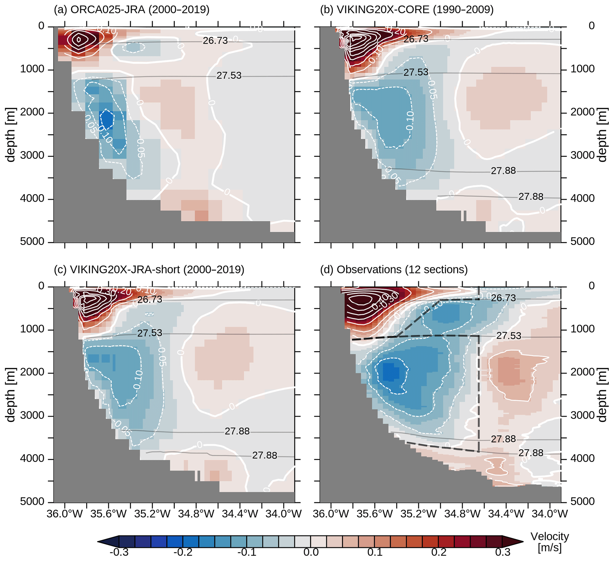
Figure 16Mean along-shore velocity (m s−1) section at 11∘ S for (a) ORCA025-JRA, (b) VIKING20X-CORE, (c) VIKING20XJRA-short and from (d) 12 observational ship sections in the periods 2000–2004 and 2013–2019 with σ0 isolines. Dashed boxes in (d) indicate the area taken into account for NBUC and DWBC transport calculations.
Measurements and long-term monitoring of the WBC system off Brazil have been motivated by the concentration of the northward upper-ocean flow in the NBUC (Hummels et al., 2015). They are part of the “Tropical Atlantic Circulation and Overturning at 11∘ S” (TRACOS) array (Herrford et al., 2021), which consists of bottom pressure observations at 300 and 500 m depth since 2013 on both sides of the basin in order to obtain an AMOC estimate, the mentioned long-term western boundary array (since 2000, but with a gap between 2004 and 2013) and current observations at the eastern boundary off Angola since 2013. Rühs et al. (2015) show that the NBUC transport can be used as an indicator for the upper branch of the AMOC if the horizontal wind-driven circulation is also accounted for. In addition to the northward return flow associated with the AMOC, the NBUC also carries most of the equatorward flow related to the South Atlantic Subtropical Cell (Schott et al., 2004). Figure 16 shows that the general structure of the WBC system is visible in all experiments. The NBUC with its subsurface maximum and the DWBC below already exist in ORCA025-JRA. The eddy-rich configurations better represent the elongated subsurface core of the NBUC and the wider, eddying (cf. Fig. 15a) DWBC, merging with a recirculation pattern offshore of the (deeper part of the) NBUC. The representation of the water masses (here indicated by the density lines) appears quite well. Model transports are usually within the standard deviations of the observational estimates based on the moorings but are generally too weak at low resolution and by one-third (NBUC) and two-thirds (DWBC) too strong for VIKING20X-CORE (Table 7).
It is interesting to note and a guidance for future model–observation comparisons that even for a well-covered section (with 12 ship-based observations) a detailed temporal selection of model output can be important depending on the variability of the system in question (Schwarzkopf, 2016). While the values deducted from the moorings show a good agreement with the ship sections for the NBUC, those for the DWBC are off by more than 10 Sv (Table 7, Fig. 17d, e). This is due to the fact that the ship-based estimate is biased by intra-seasonal variability (Hummels et al., 2015), with ship sections often conducted during times of maximum southward flow that often only last for a few days (Fig. 17e, especially during 2000–2004). It is important to emphasise that the simulations capture the strong variability and confirm the apparent discrepancy between the long-term mean and the subsampled values.
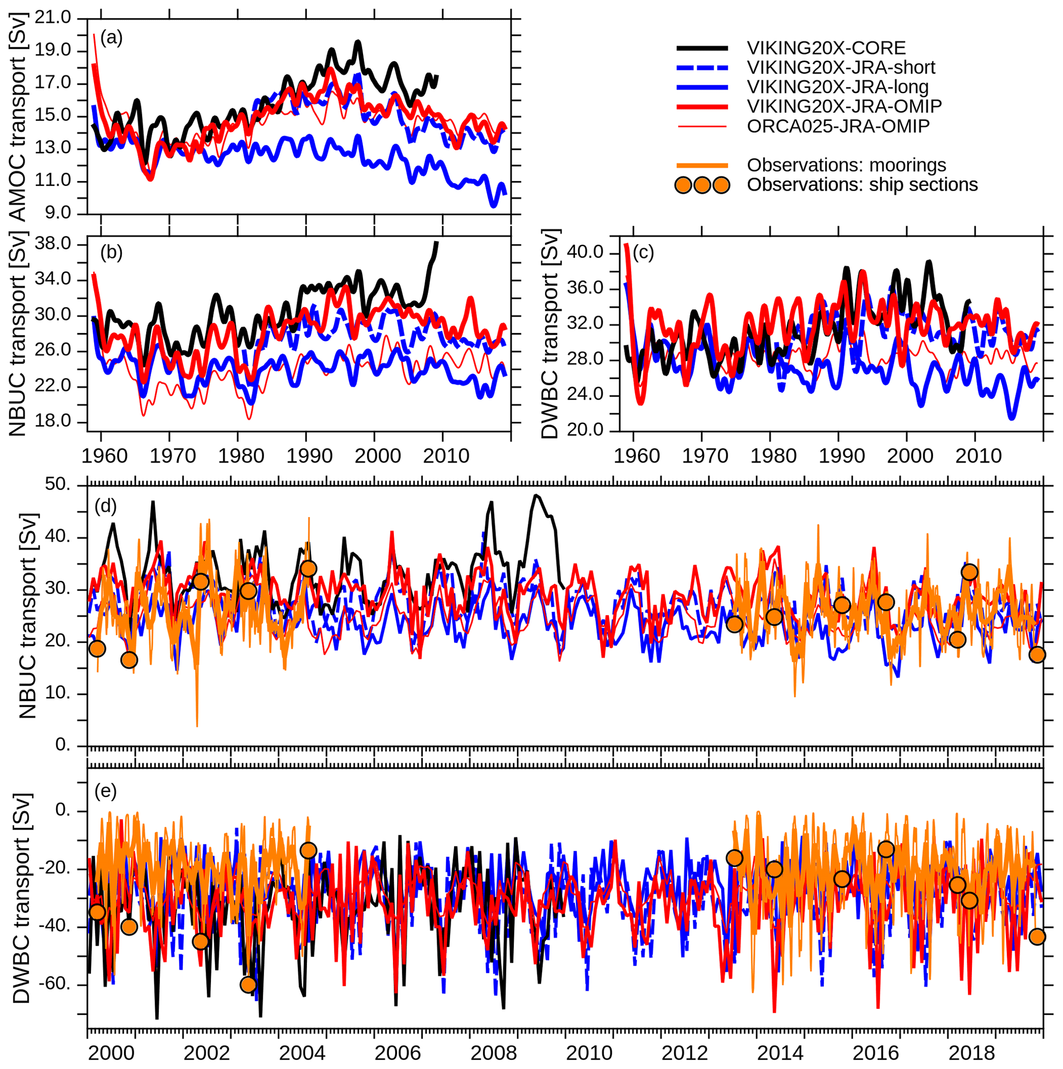
Figure 17Time series of interannually filtered (a) AMOC, (b) NBUC and (c) DWBC transports at 11∘ S; monthly averages of positive (north-northeastward) NBUC and negative (south-southwestward) DWBC transports (see Table 7 for details of the definitions) are given in (d) and (e) together with mooring-based (orange curves; thick monthly, thin 2.5 d averages) and ship-based observations (orange dots).
Figure 17a shows the temporal evolution of the AMOC at 11∘ S. In contrast to the one at 26.5∘ N (Fig. 5a), it shows a minimum in the late 1960s which is in particular the case in VIKING20X-JRA-OMIP that started one decade earlier from rest. In the following decades, the experiments (apart from VIKING20X-JRA-long) simulate an increase into the 1990s with a decline thereafter.
Transports of the NBUC and DWBC (Fig. 17b, c) are less robust among the experiments and show no clear or consistent multi-decadal evolution. In consequence, trends over limited periods are less consistent. Apart from the trends, both AMOC and NBUC are significantly correlated between individual experiments on interannual timescales with r values of up to 0.85. In contrast, DWBC transports are rarely correlated.
Within individual experiments, there is no robust co-variability of the AMOC with NBUC (or DWBC) transports. Some (e.g. VIKING20X-JRA-OMIP) show significant correlations while others (e.g. VIKING20X-JRA-long) do not (here not shown).
Table 8Mean and standard deviation based on monthly data of the AMOC transport (in Sv) at 34.5∘ S for the period 1990–2009 and subsampled in the observational period (Obs.) (for VIKING20X-CORE only the overlapping year 2009 is used).
* The observational period covers the years 2009/2010 and 2013–2017.
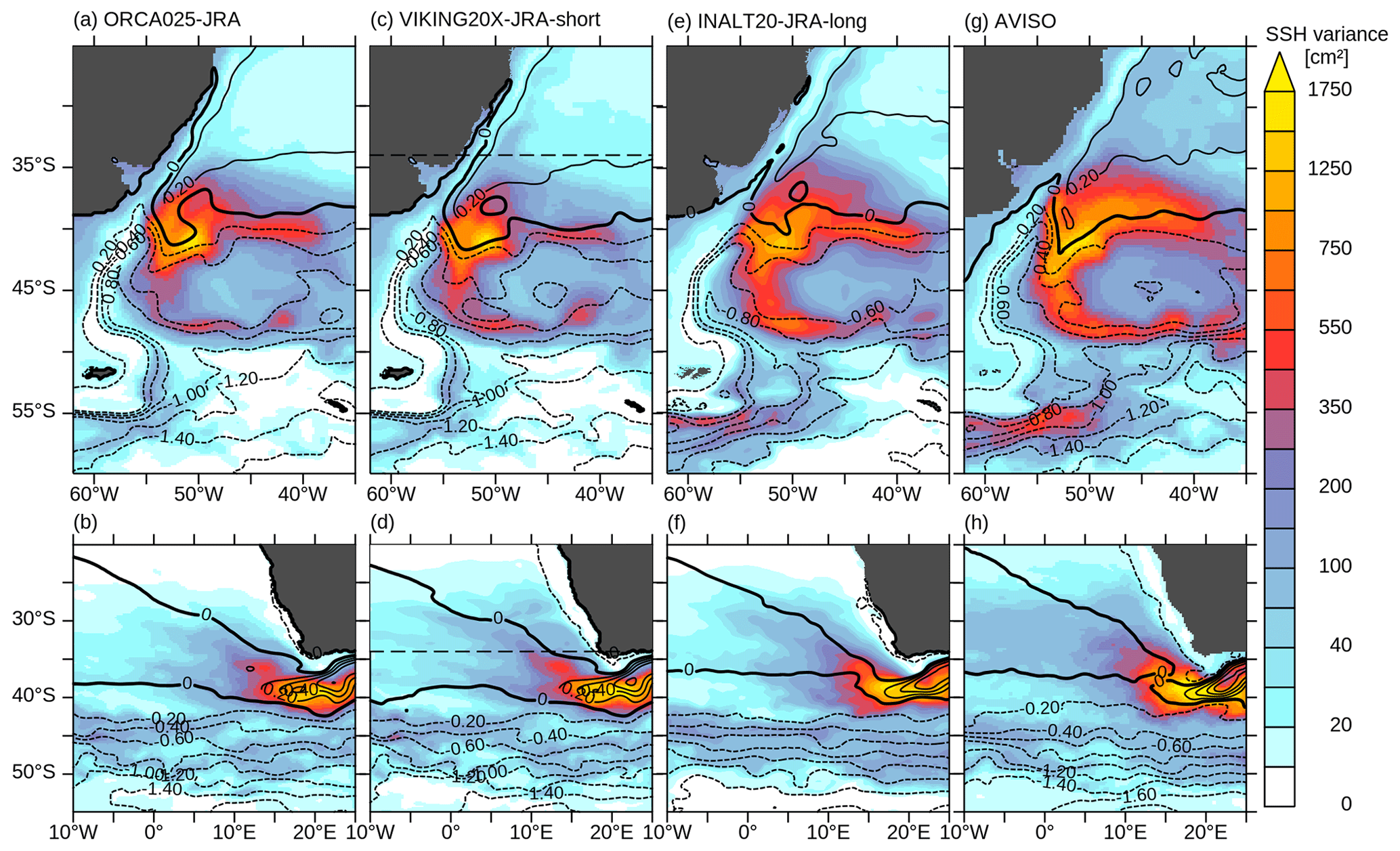
Figure 18Sea surface height in the Brazil–Malvinas confluence zone (upper row) and west Agulhas region (lower): 1990–2009 mean (contours, in m) and variance (shaded, in cm2) in (a, b) ORCA025-JRA, (c, d) VIKING20X-JRA-short, (e, f) INALT20-JRA-long and (g, h) from satellite altimetry. Dashed lines in (c) and (d) mark the southern boundary of the nested region in VIKING20X.
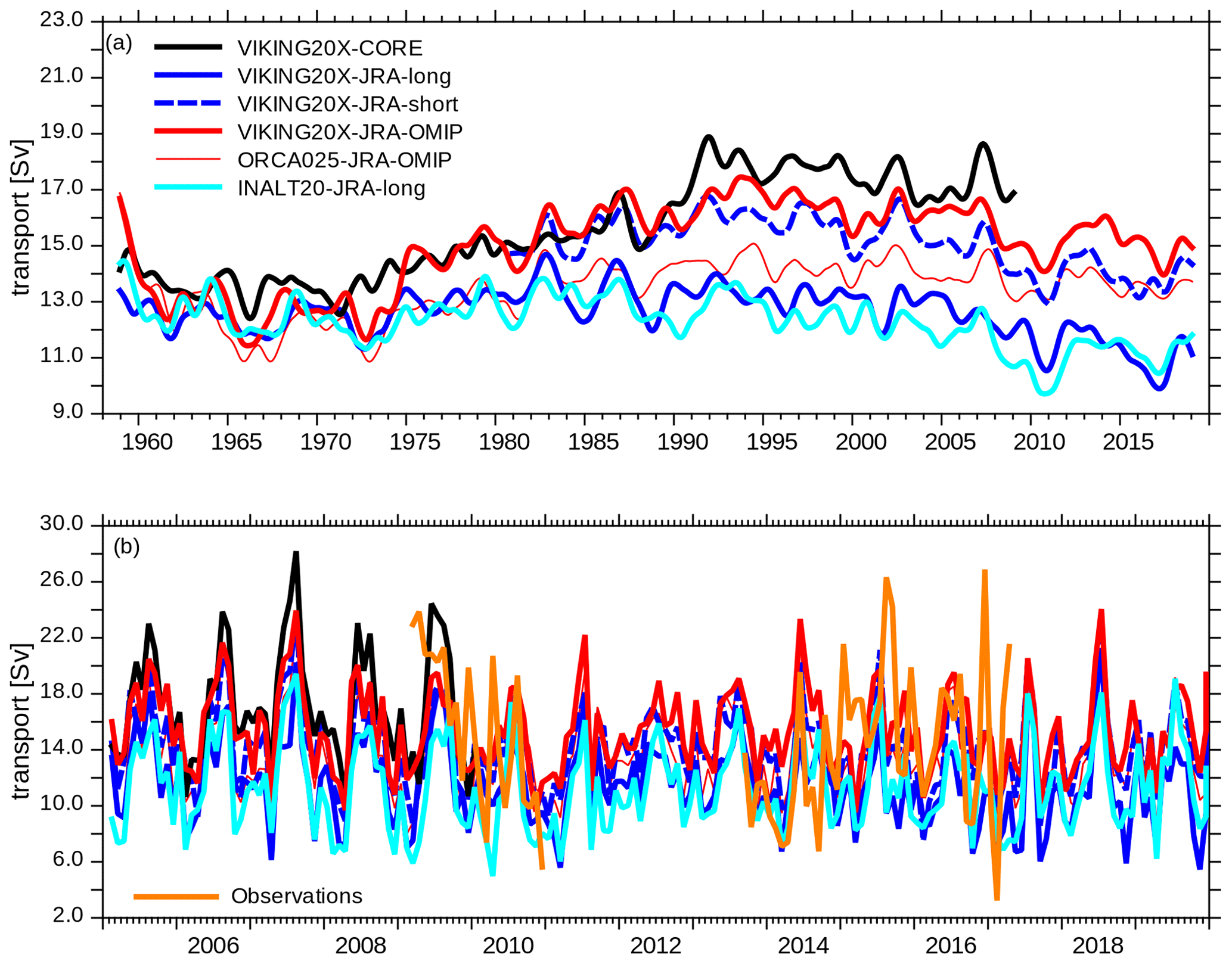
Figure 19Time series of the AMOC strength at 34.5∘ S (a) interannually filtered and (b) monthly averages for the most recent 15 years with observations from Meinen et al. (2018) (orange).
4.4 Subtropical South Atlantic
Entering the subtropical South Atlantic brings us closer to the southern boundary of VIKING20X's high-resolution nest. In the following we explore the ability of the nested configuration to simulate the mesoscale circulation in the Agulhas Current system and the Brazil–Malvinas confluence and whether the host model is capable in correctly simulating the transports at the SAMOC observations which are placed just outside the nested area. For comparison we use INALT20 (Schwarzkopf et al., 2019), a configuration that is in large parts (in particular resolution and atmospheric forcing) similar to VIKING20X, but with an eddy-rich nest reaching into the Southern Ocean and into the western Indian Ocean.
Figure 18 confirms the general ability of VIKING20X to simulate parts of the mesoscale in the vicinity of the southern nest boundary. It is logical that the variability in the Brazil–Malvinas confluence in VIKING20X-JRA-short is lower and rather comparable to ORCA025-JRA (Fig. 18a and b), given the fact that these latitudes are only represented on the host grid at ∘ resolution. In addition to the mesoscale signal, Schwarzkopf et al. (2019) demonstrated that the correct representation of the confluence region has consequences for the structure and transport of the Malvinas Current. The picture is similar for the path of Agulhas rings. Here, the formation process in the retroflection of the Agulhas Current south of Africa is outside the VIKING20X nest. Since Agulhas rings are generally represented in ORCA025 (Schwarzkopf et al., 2019), they also enter the nest. The difference compared to a configuration fully resolving the Agulhas Current dynamics (and observations) is that ORCA025 simulates overly regular Agulhas rings. This is seen in a more confined SSH pattern in Cape Basin (Fig. 18b and d) as an indicator of an overly regular pathway into the South Atlantic.
The AMOC at 34.5∘ S shows the same evolution as the one in the North Atlantic, with a maximum in the 1990s (in some experiments relative and generally less pronounced) and a weakening thereafter if simulated under JRA55-do forcing (Fig. 19a). Even though the representation of the mesoscale is different as discussed above, the mean interannual variability and long-term trend in INALT20-JRA-long and VIKING20X-JRA-long are remarkably comparable. By comparing the transports in VIKING20X-JRA-long with those in ORCA025-JRA, and VIKING20X-JRA-OMIP with ORCA025-JRA-OMIP, we notice a similar resolution effect as seen in the North Atlantic (Table 8). Compared to the (temporally limited) observations by Meinen et al. (2018), most experiments underestimate the mean AMOC transport through the section. However, all VIKING20X experiments are in the range of the standard deviations with respect to the monthly variability. The representation of Agulhas rings even in the eddy-present ORCA025 resolution could be an important prerequisite for the realistic AMOC variability. The interannual variability is correlated among experiments, with r values of for example 0.8 between VIKING20X-JRA-long and VIKING20X-JRA-OMIP, similar to the other latitudes (here not shown). Interestingly, this is also the case when mesoscale variability is better resolved. INALT20-JRA-long correlates interannually with VIKING20X-JRA-OMIP at r=0.81. Given the fact that the generation of Agulhas rings is a highly stochastic process (Biastoch et al., 2009), this shows that the interannual variability of the AMOC at 34.5∘ S has a significant deterministic component by the atmospheric forcing.
Our results show that a “realistically” configured ocean hindcast in a configuration like VIKING20X is well suited for simulating the large-scale circulation dynamics in the Atlantic Ocean. Once the mesoscale is resolved by an adequate resolution over the full model domain and the model is driven by a realistic and balanced atmospheric forcing, many aspects of the simulated wind-driven and thermohaline circulation compare very well with observations. These include the large-scale structure of the mean flow, the distribution and strength of mesoscale eddies, WBC structures, and individual current systems. There is good agreement between model and observations in terms of velocity structures and integral transports, even of their temporal variability and trends. Because of the strong impact of the wind forcing, the role of the atmospheric forcing dataset cannot be underestimated for such an ocean-only model. The shift of the ocean model community from CORE forcing (Large and Yeager, 2009) to the more highly resolved and updated JRA55-do forcing (Tsujino et al., 2018) is an important change. CORE was known to enhance individual wind systems such as the equatorial trades or the Southern Hemisphere westerlies (Large and Yeager, 2009; Brodeau et al., 2010), which can be the cause for generally higher WBC transports in VIKING20X-CORE. Together with a different subpolar–subarctic freshwater budget, e.g. by the precipitation components and river input, this leads to a stronger and more stable AMOC, which is reflected in regional components.
Even though WBC transports and AMOC strength are generally enhanced at eddy-rich resolution, other aspects are remarkably independent. One example is the decadal transport variability of the subpolar gyre. It is important to note that our configurations do not allow the effect of eddies to be isolated. We acknowledge that the eddy-present ORCA025 does not use any eddy parameterisation; it explicitly simulates “some” (the larger-scale) part of the mesoscale spectrum, while neglecting others. This dilemma is similar to many modern eddy-present configurations performed for CMIP6 (Hewitt et al., 2020). And yet, although the level of mesoscale variability significantly increases from to ∘, the interannual variability of the AMOC appears quite robust. Features like the 2010 minimum can be simulated well at eddy-present resolution, pointing to an ability of the CMIP6 suite to simulate an important part of the mesoscale contribution to the AMOC. On decadal timescales differences between the two resolutions are more evident as a result of the better ability of VIKING20X to simulate key aspects of the thermohaline component such as overflow, entrainment and convection.
More caution is required with respect to the thermohaline-driven part of the circulation. Although we see an improvement in the features of deep convection regions in the Labrador and Irminger Seas from to ∘, the amount of potentially produced upper NADW (here quantified in terms of the mixed layer volume) appears remarkably robust. In contrast, for the backbone of the AMOC, the overflow across the Greenland–Scotland Ridge is clearly improved with enhanced horizontal resolution. And still, the underestimation of the lower NADW at 53∘ N confirms that the entrainment of ambient water masses into the overflow along its downward descent while circling the subpolar gyre even simulated at high resolution is subject to spurious mixing. The simulations cannot maintain the observed high densities to yield the correct transports in the densest levels. The underrepresentation of the lower NADW throughout the whole Atlantic still remains an important challenge in z-coordinate models (Legg et al., 2006), even though an eddy-rich resolution is an important improvement. As a cautionary note, we point to the study by Colombo et al. (2020), who showed that a higher vertical resolution does not automatically enhance the spreading of dense overflows and sometimes even leads to the contrary effect.
For the estimation of the decadal variability and any long-term trend of the AMOC, realistically distributed components of the freshwater budget are crucial because of the enhanced sensitivity of ocean-only models to freshwater fluxes, in particular their corresponding subpolar freshwater budget (Griffies et al., 2009; Behrens et al., 2013). Because of this sensitivity, AMOC trends from internal variability and external forcing are usually difficult to quantify against model-related drifts. The modelled trends depend on artificial choices of the prescribed freshwater fluxes, such as the required strength of the SSS restoring or (as in our case) a global balance of the freshwater budget. Since these parameter or forcing choices are not well constrained and may even interfere with each other, the quantification of the AMOC evolution over the past decades from hindcast simulations remains a challenge. Any quantification of global-warming-related trends induced by the atmospheric forcing is compromised by the underlying model drift.
Beyond the description and verification of the VIKING20X set of experiments, our main objective is to test whether changes in the zonally integrated AMOC are also evident at the more local scale of regional current systems. In the remaining discussion, we address this task by answering three questions: (1) how coherent are AMOC changes across latitudes throughout the Atlantic Ocean? (2) Are AMOC trends detectable in regional current systems? And if so, (3) can regional observations help to verify and confirm modelled AMOC trends?
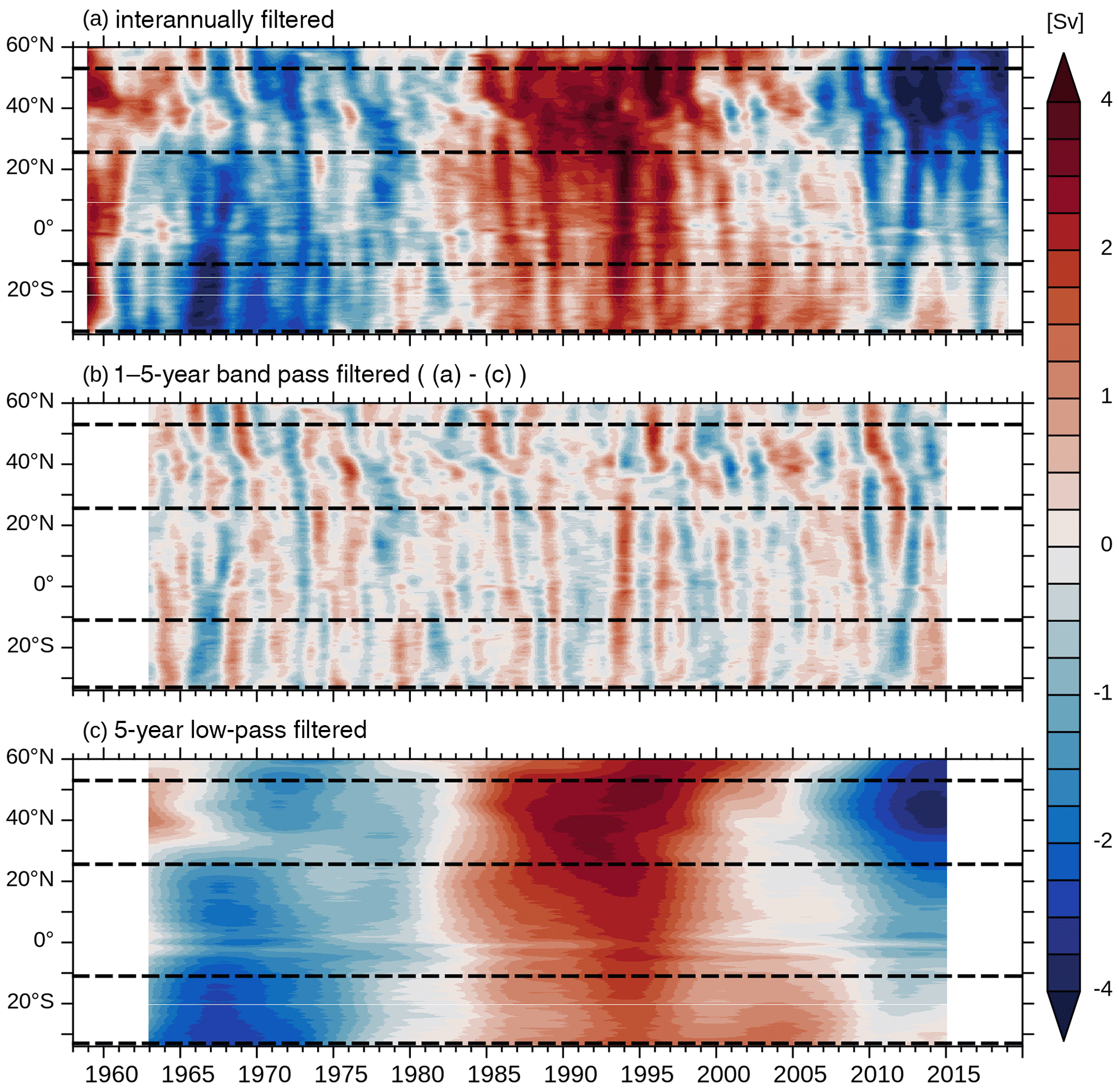
Figure 20Hovmöller diagrams of AMOC anomalies in density coordinates given as (a) interannually, (b) bandpass and (c) 5-year low-pass filtered time series of the maximum strength between σ2=36 and 37 from VIKING20X-JRA-OMIP. Dashed horizontal lines indicate latitudes considered in this study.
5.1 How coherent are AMOC changes across latitudes throughout the Atlantic Ocean?
Most VIKING20X experiments (apart from VIKING20X-JRA-long, which shows a continuous decline of the AMOC throughout the whole hindcast period) show a similar evolution of the AMOC, with an increase towards the mid-1980s and 1990s, and a decline thereafter. This is shown for VIKING20X-JRA-OMIP as an example (Fig. 20). The Hovmöller diagram (here given in density coordinates to correctly address the subpolar North Atlantic) shows the evolution and the spreading of AMOC anomalies throughout the Atlantic Ocean. Consistent with earlier findings, the strongest anomalies arise in the subpolar gyre as a response to a decadally varying heat and freshwater forcing (Biastoch et al., 2008a; Yeager and Danabasoglu, 2014). On decadal timescales, this signal is evident at all latitudes, but with decreasing amplitudes towards the south (cf. Fig. 20a and c, but also Figs. 5a, 17a, and 19a). Other signals such as the minimum in the late 1960s or the maximum in the 2000s seem to be of southern origin and remain restricted until ∼ 20∘ N. AMOC anomalies appearing on shorter timescales add interannual “noise” to this decadal evolution. We identify both latitudinally restricted changes of interannual variability and also anomalies propagating from the north or the south throughout the full Atlantic Ocean. These anomalies are either caused by local wind changes inside the high-resolution nest itself or provided from the eddy-present host grid outside of the nested domain, which rapidly propagate north- and southward via topographic and shelf waves along both sides of the Atlantic Ocean (Getzlaff et al., 2006; Biastoch et al., 2008b). In the Hovmöller diagram the associated patterns are only slightly slanted, indicating the fast wave propagation. Besides the typical equatorial discontinuity, anomaly propagation is significantly delayed at the transition between the subpolar and the subtropical North Atlantic because of the complex exchange between the gyres ∼ 40–50∘ N (Zou et al., 2019).
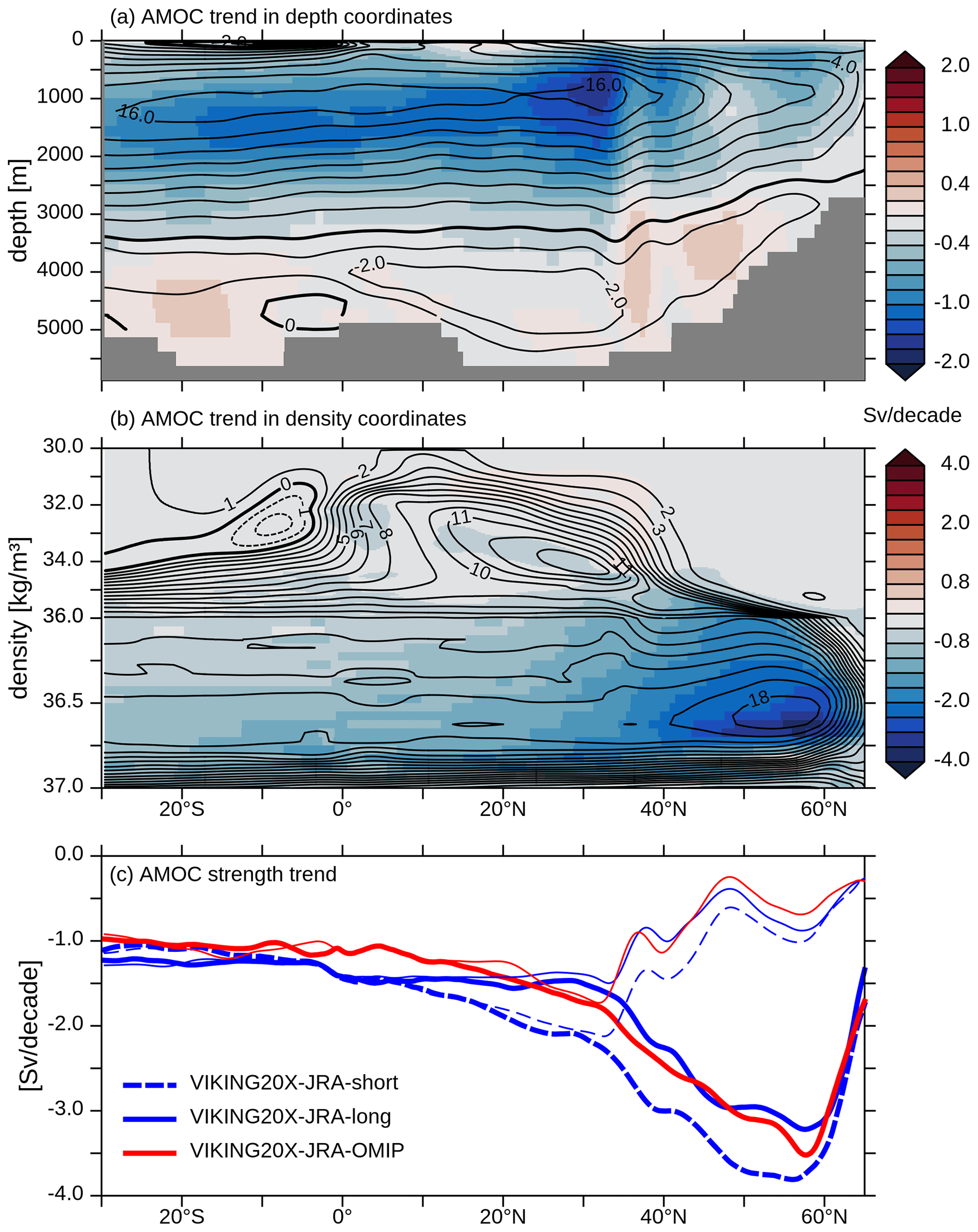
Figure 21Mean (contours, in Sv) and linear trend (shading, in Sv per decade) in the AMOC for the period 2000–2019 in VIKING20X-JRA-OMIP (a) in depth and (b) density (σ2) coordinates. Panel (c) shows the linear trend of the vertical maximum in the AMOC in depth coordinates below 400 m (thin) and in density coordinates below σ2=36 (thick). All fields are meridionally smoothed with a Hanning filter of 10∘ window size.
Table 9Linear trends (Sv per decade, all based on monthly averaged data) in AMOC strength (in depth or density coordinates) and western boundary current transports at different latitudes for the period 2000–2019 from the three experiments in VIKING20X under JRA55-do forcing. Observational estimates cover different periods, as indicated.
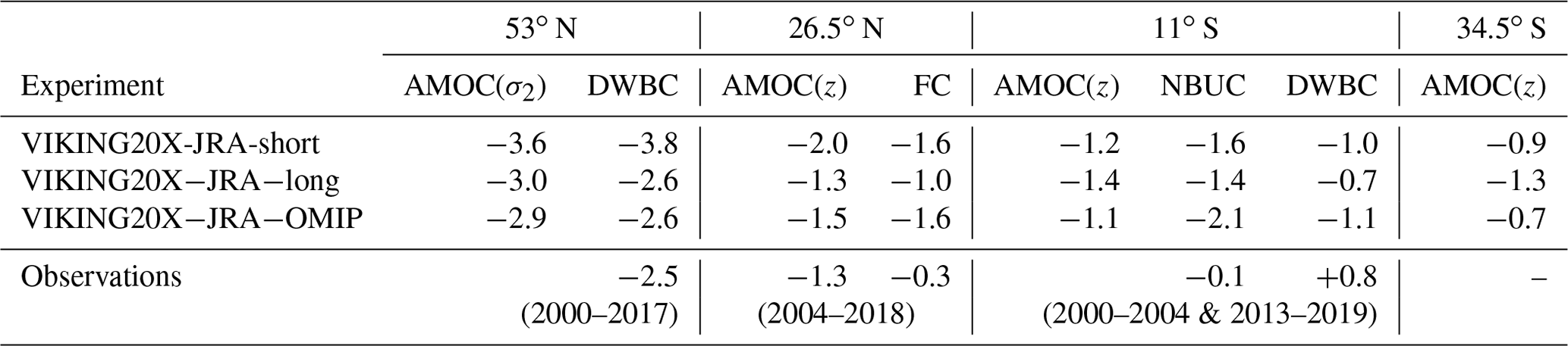
If we now focus on the “trend” of the AMOC over the past two decades (Fig. 21), which itself is part of a multi-decadal evolution, VIKING20X-JRA-OMIP shows a coherent spin-down of the NADW cell. The general evolution of the other experiments is similar but differs in the strength of the decline (Fig. A2). Since all experiments are based on the same atmospheric forcing, differences in the decline are due to choices of the freshwater application and the initialisation. Changes in the overflow and subpolar deepwater formation provide the main origin for the AMOC evolution, and consequently the decline (once provided in density coordinates to correctly address the subpolar North Atlantic, Fig. 21b) is strongest north of ∼ 40–45∘ N. Quantitatively, the AMOC decline peaks at ∼ 60∘ N, the latitude close to the southern tip of Greenland, until which the overflow has entrained most of its ambient water masses (Fig. 21c). South of the transition towards the subtropical North Atlantic, at around 35∘ N, the decline in VIKING20X-JRA-long and VIKING20X-JRA-OMIP is consistent at 1–1.5 Sv per decade, even though their mean AMOC strength differs by more than 4 Sv. (Fig. 21c; see also Table 2). VIKING20X-JRA-short features a stronger decline since it starts from a relatively high value as a result of the preceding CORE forcing and obviously experiences a spin-down from the high level of the CORE forcing. Owing to the general spin-down of the NADW cells we conclude that decadal and longer-term AMOC trends could be estimated throughout all latitudes of the North and South Atlantic but with different strengths.
5.2 Are AMOC trends detectable in regional current systems?
Apart from the basin-wide estimate at 26.5∘ N, regional observations exist and contribute long-term observations of key components of the AMOC. In this analysis we have focused on three time series: the WBC array at 53∘ N monitoring DWBC transports at the exit of the Labrador Sea, the transport through the Florida Strait as an important part of the upper branch of the AMOC, and the WBC array at 11∘ S in which both the upper and the deep branches of the AMOC are assumed to be concentrated along the western boundary.
It is intriguing that the DWBC trend at 53∘ N is able to capture the AMOC trend calculated in density coordinates within 10 %–15 % (Table 9). This correspondence even holds for the stronger trends in VIKING20X-JRA-short. This agreement confirms the high potential of WBC measurements at 53∘ N (Fischer et al., 2004; Zantopp et al., 2017; Handmann et al., 2018) to truly monitor changes of the AMOC in the subpolar North Atlantic (Böning et al., 2006).
For the transport through the Florida Strait and its agreement with AMOC changes at 26.5∘ N, we get a different picture: in VIKING20X-JRA-short and VIKING20X-JRA-long, the decline of the Florida Current is about 75 %–80 % of the decline of the AMOC, in contrast to VIKING20X-JRA-OMIP where it is stronger. This may indicate that the Florida Current could act as a general precursor of the AMOC trend but is unable to exactly quantify it. This is confirmed by the observations themselves, where the Florida Current decline represents just 15 % of the AMOC decline. It is obvious that the Florida Current is not just a simple closure of Sverdrup dynamics but rather is shielded by the shallow bathymetry west of the Bahamas and fed through the Gulf of Mexico, with upstream anomalies determining its transport (Hirschi et al., 2019). This may also explain the disagreement between modelled and observed trends of the Florida Current, even though both show comparable mean transports (Table 6).
At 11∘ S, AMOC changes cannot be indicated by changes in the WBC system alone but also require the consideration of interior (Ekman) and eastern components (Rühs et al., 2015; Herrford et al., 2021). Although the experiments show a robust AMOC decline of about 15 %, their NBUC changes are much less consistent and do not necessarily reflect the AMOC: for VIKING20X-JRA-long the NBUC trend is equal to the AMOC trend, while for VIKING20X-JRA-OMIP the NBUC trend is almost twice as large as the AMOC trend. For the DWBC instead, trends in VIKING20X-JRA-short and VIKING20X-JRA-OMIP fit to that of the AMOC, whereby VIKING20X-JRA-long simulates a 50 % weaker trend than for the AMOC. While the signs of NBUC and DWBC trends still point towards a spin-down of the AMOC cell, an exact quantification of the reduction remains challenging. Apart from changes in the interior, not represented by the boundary current measurements, the disagreement can also be attributed to the overlying wind-driven subtropical cell (viz. counter-clockwise circulation in the upper few 100 m in Figs. 3 and 21b), at this latitude requiring the addition of the wind-induced gyre circulation for the interpretation of thermohaline-driven AMOC changes (Rühs et al., 2015). We also have to acknowledge that the large variability of transports associated with mesoscale structures and the large gaps in the observational record between 2004 and 2013 adds another line of complication and requires longer time series to draw consistent conclusions. At 34∘ S, we note a disagreement of AMOC trends in the different experiments. As shown by Fig. 20, AMOC anomalies are entering from the south and interfere with the anomalies arriving from the north. These may have an impact on the calculation of longer trends.
5.3 Can regional observations help to verify modelled AMOC trends?
Together with the AMOC measurements at 26.5∘ N, the WBC array at 53∘ N provides the longest observational time series. As shown above, the latter has (according to the model) good potential to provide trends of the basin-scale AMOC. The observational AMOC estimate at 26.5∘ N indicates a decline that is in the range of all three experiments (Table 9), again with a stronger trend in VIKING20X-JRA-short. We note that the observational AMOC trend has to be taken with caution since the evolution of the AMOC measured at RAPID does not show a continuous decline but rather a strong minimum around 2010 and a stabilisation thereafter (Fig. 5a) (Moat et al., 2020). A strong argument for a realistic AMOC trend in the past two decades emerges from the comparison at 53∘ N. Both VIKING20X-JRA-long and VIKING20X-JRA-OMIP are within 0.1 Sv of the observed reduction of the DWBC transport of 2.5 Sv per decade (Table 9) and hence seem to realistically simulate the decline of the subpolar AMOC. For the subtropical North Atlantic at 26.5∘ N this reduces to 1.3 Sv per decade, again with VIKING20X-JRA-long and VIKING20X-JRA-OMIP realistically representing the AMOC as derived from RAPID.
Apart from the observation–model comparison, additional insight comes from the Ocean Model Intercomparison Project 2 (OMIP-2), in which models performed six subsequent cycles under JRA55-do forcing. According to Tsujino et al. (2020), the ensemble average of 11 models, performed with different numerical code bases and mainly configured at eddy-parameterising (few at eddy-present) resolutions, show a linear trend of −1.19 Sv per decade over the time frame 2000–2018 at 26.5∘ N, which is weaker than RAPID. We cannot conclude if the stronger decline simulated by VIKING20X-JRA-OMIP and VIKING20X-JRA-long is caused by the better representation of mesoscale eddies, as indicated by the resolution dependence throughout this study, or by the details of the freshwater flux application. An important factor could be the sixth cycling of the simulations through the forcing period done for OMIP-2. While six cycles are not yet achievable at such high resolution, the comparison of the first and the second cycles of ORCA025-JRA-OMIP already suggests that this may play a role. The trend in ORCA025-JRA-OMIP reduces from −0.88 Sv per decade in the first cycle to −0.67 in the second cycle. On the other hand, it is quite foreseeable that the overall strength of the AMOC and the related water masses may also drift away from the observations, causing a general reduction of the AMOC strength and its key components (Fig. 8).
Even though we find good agreement with estimates at 26.5 and 53∘ N, we can not conclusively assess how much of the trends simulated by the different experiments are still related to the model settings. We can also not be entirely sure whether the trends provided by the JRA55-do forcing are realistic. If we consider VIKING20X-JRA-OMIP as the most promising simulation given good agreement of mean transports, it is clear that the AMOC is subject to multi-decadal variability with a stable evolution in the 1960s and 1970s, an increase towards the mid-1990s and a decline thereafter. For the past two decades our experiments suggest that the AMOC (in density coordinates) in the subpolar North Atlantic was subject to a decline of up to 3 Sv. For the subtropical North Atlantic and further south this decreases to about 1.5 Sv and less. This is generally in line with a compilation of proxy observations presented by Caesar et al. (2021). On a longer timescale, it also fits the 4 Sv decline from the 1950s and 1960s towards the recent decade indicated by an SST-based proxy (Caesar et al., 2018).
What is needed to better quantify trends in future experiments and limit the influence of model drift? Apart from further improvements of ocean model configurations, it is clear that multi-decadal hindcasts would directly benefit from a better closure of the heat and freshwater budget. This can only be achieved up to a certain degree since the fluxes are by construction less variable due to the prescribed atmospheric state. Further relaxation of the bulk formulae or a move towards coupled atmosphere–ocean models may help. While the latter are now routinely available, even at basin-scale mesoscale resolution (Matthes et al., 2020), additional “constraints” such as the “partial coupling” approach described by Thoma et al. (2015) could be a potential solution to re-introduce the interannual to multi-decadal hindcast “timing” into coupled experiments.
This study focuses on a limited set of long-term observations. In addition, a number of historic ocean observations exist, from individual measurements dating back to the 19th century, repeated ship sections during the WOCE era in the 1990s, to a drastic increase through satellite measurements and autonomous instruments such as ARGO in the 2000s. Ocean modellers usually make use of those for model initialisation or verification. More systematic approaches to combine model and data through assimilation are powerful but also fail in terms of their ability to exactly quantify the required trends (Karspeck et al., 2015; Jackson et al., 2019). A novel route in this respect that has only recently begun to be explored employs data science approaches. These methods have been demonstrated to push the limits of the interpretation of big data and provide insight not only into patterns and distributions but also into the interpretation (and ultimately the understanding) of dynamics (Sonnewald et al., 2019; Aksamit et al., 2020; Reichstein et al., 2019). Nevertheless, our results demonstrate the value and importance of thoroughly and carefully adjusting forcing, grid resolution and settings of “classic” ocean models to the tasks of simulating the AMOC and filling observational gaps for the benefit of an improved understanding of the ocean.
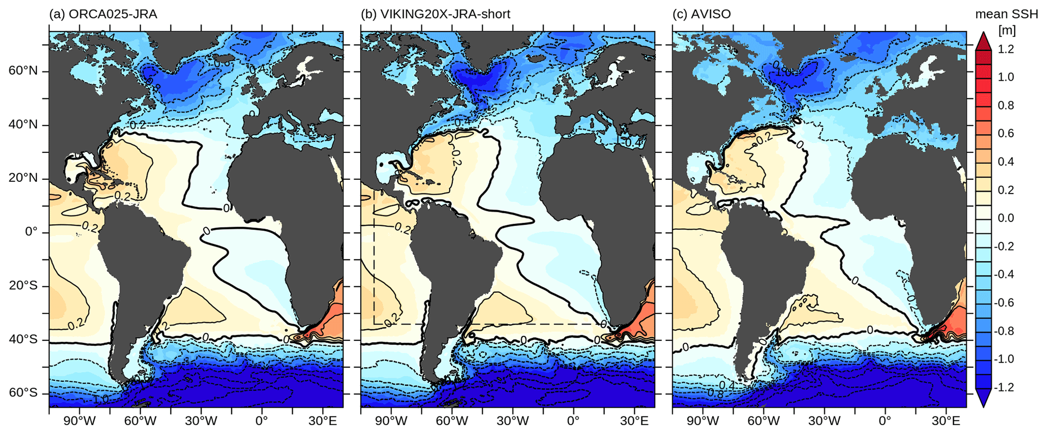
Figure A1Mean (1993–2019) sea surface height (in m) in (a) ORCA025-JRA, (b) VIKING20X-JRA-short and (c) satellite altimetry.
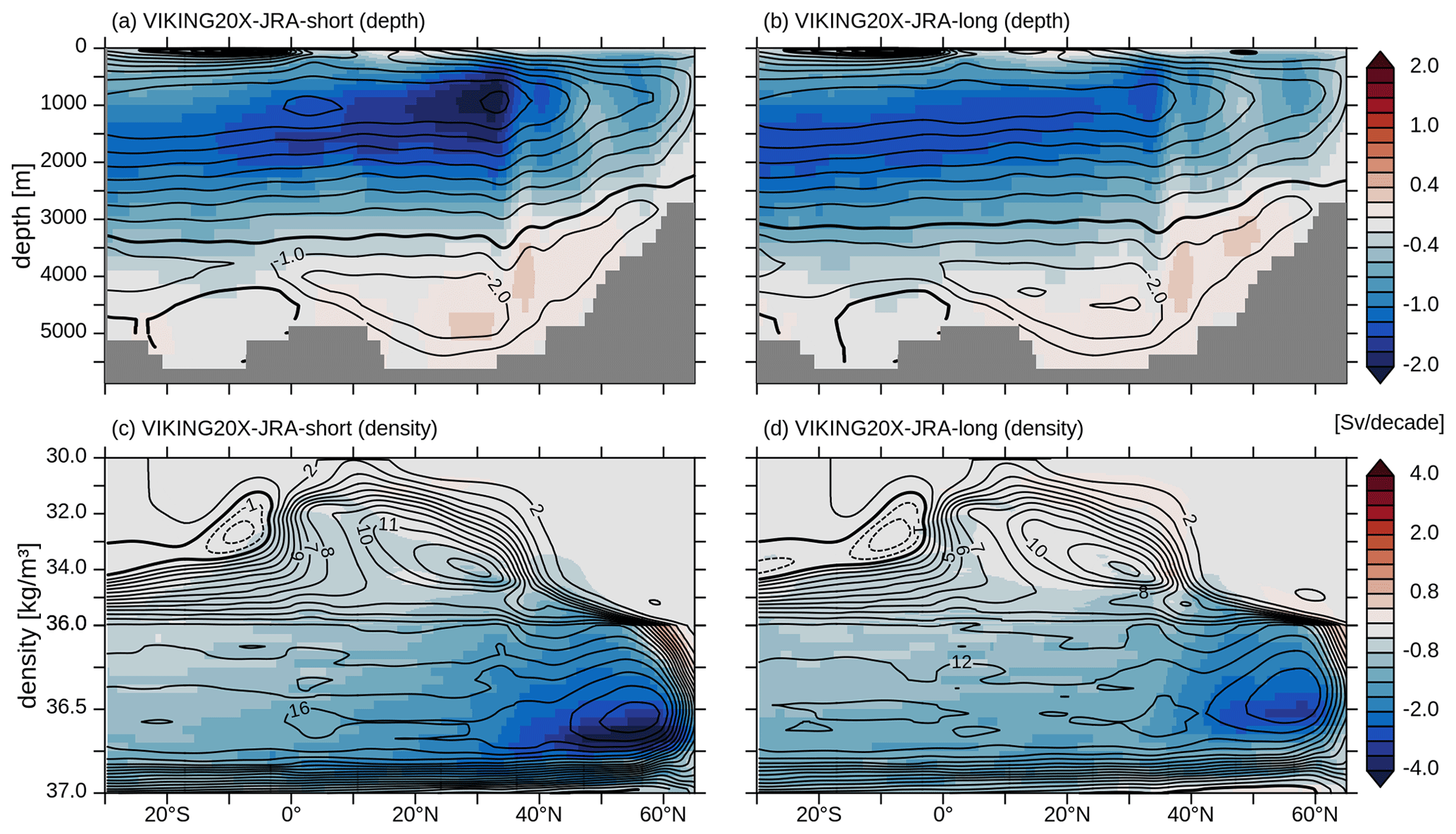
Figure A2Mean (contours, in Sv) and linear trend (shading, in Sv per decade) in the AMOC in (a) and (b) depth and (c) and (d) density (σ2) coordinates for the period 2000–2019 for VIKING20X-JRA-short and VIKING20X-JRA-long. All fields are meridionally smoothed with a Hanning filter of 10∘ window size.
The NEMO code is available at https://forge.ipsl.jussieu.fr/nemo/svn/NEMO/releases/release-3.6 (NEMO System Team, 2021). Our experiments are based on revision 6721. For reproducibility of all results, code modifications and the scripts as well as all data required to produce the figures are made available through GEOMAR (https://hdl.handle.net/20.500.12085/a8f98a1a-473f-11ea-a036-c81f66eb46c3, Biastoch et al., 2021). Python code of the runoff remapping tool can be accessed through https://oceanrep.geomar.de/53895/ (Martin, 2021). Additional model output is provided on request.
AB and CWB defined and guided the overall research problem and methodology. FUS and KG developed and performed the ocean model simulations. FUS, KG, SR, TM, MS, TS, PH and RH contributed analyses and figures for the individual parts. All co-authors discussed the analyses and contributed to the text.
The authors declare that they have no conflict of interest.
Publisher's note: Copernicus Publications remains neutral with regard to jurisdictional claims in published maps and institutional affiliations.
The ocean model simulation was performed at the North German Supercomputing Alliance (HLRN) and on the Earth System Modelling Project (ESM) partition of the supercomputer JUWELS at the Jülich Supercomputing Centre (JSC). We thank the NEMO system team for support. The Florida Current cable and section data are made freely available on the Atlantic Oceanographic and Meteorological Laboratory web page (https://www.aoml.noaa.gov/phod/floridacurrent/, last access: 11 November 2020) and are funded by the DOC-NOAA Climate Program Office – Ocean Observing and Monitoring Division.
This research has been supported by the German Federal Ministry of Education
and Research (grants SPACES-CASISAC (03F0796A) and RACE Regional Atlantic Circulation and Global Change (03F0729C)). It has also received funding from the Initiative and Networking Fund of the Helmholtz Association through the project “Advanced Earth System Modelling Capacity (ESM)” and the European Union's Horizon 2020 research and innovation programmes under grant agreement nos. 818123 (iAtlantic) and 817578 (TRIATLAS).
The article processing charges for this open-access publication were covered
by the GEOMAR Helmholtz Centre for Ocean Research Kiel.
This paper was edited by Matthew Hecht and reviewed by two anonymous referees.
Aksamit, N. O., Sapsis, T., and Haller, G.: Machine-Learning Mesoscale and Submesoscale Surface Dynamics from Lagrangian Ocean Drifter Trajectories, J. Phys. Oceanogr., 50, 1179–1196, https://doi.org/10.1175/JPO-D-19-0238.1, 2020. a
Amante, C. and Eakins, B.: ETOPO1 1 Arc-Minute Global Relief Model: Procedures, Data Sources and Analysis, NOAA Tech. Memo. NESDIS NGDC-24, p. 19, https://doi.org/10.1594/PANGAEA.769615, 2009. a
Arakawa, A. and Hsu, Y.-J. G.: Energy Conserving and Potential-Enstrophy Dissipating Schemes for the Shallow Water Equations, Mon. Weather Rev., 118, 1960–1969, 1990. a
Baltazar-Soares, M., Biastoch, A., Harrod, C., Hanel, R., Marohn, L., Prigge, E., Evans, D., Bodles, K., Behrens, E., Böning, C. W., and Eizaguirre, C.: Recruitment collapse and population structure of the european eel shaped by local ocean current dynamics, Curr. Biol., 24, 104–108, https://doi.org/10.1016/j.cub.2013.11.031, 2014. a
Bamber, J. L., Tedstone, A. J., King, M. D., Howat, I. M., Enderlin, E. M., van den Broeke, M. R., and Noel, B.: Land Ice Freshwater Budget of the Arctic and North Atlantic Oceans: 1. Data, Methods, and Results, J. Geophys. Res.-Ocean., 123, 1827–1837, https://doi.org/10.1002/2017JC013605, 2018. a
Barnier, B., Madec, G., Penduff, T., Molines, J.-M., Treguier, A.-M., Le Sommer, J., Beckmann, A., Biastoch, A., Böning, C., Dengg, J., Derval, C., Durand, E., Gulev, S., Remy, E., Talandier, C., Theetten, S., Maltrud, M., McClean, J., and De Cuevas, B.: Impact of partial steps and momentum advection schemes in a global ocean circulation model at eddy-permitting resolution, Ocean Dynam., 56, 543–567, 2006. a, b, c
Behrens, E.: The oceanic response to Greenland melting: the effect of increasing model resolution, Phd. thesis, Christian-Albrechts-Universität Kiel, urn:nbn:de:gbv:8-diss-136843, 2013. a, b
Behrens, E., Biastoch, A., and Böning, C. W.: Spurious AMOC trends in global ocean sea-ice models related to subarctic freshwater forcing, Ocean Model., 69, 39–49, https://doi.org/10.1016/j.ocemod.2013.05.004, 2013. a, b, c, d
Behrens, E., Våge, K., Harden, B., Biastoch, A., and Böning, C. W.: Composition and variability of the Denmark Strait Overflow Water in a high-resolution numerical model hindcast simulation, J. Geophys. Res.-Ocean., 122, 2830–2846, https://doi.org/10.1002/2016JC012158, 2017. a
Berx, B., Hansen, B., Østerhus, S., Larsen, K. M., Sherwin, T., and Jochumsen, K.: Combining in situ measurements and altimetry to estimate volume, heat and salt transport variability through the Faroe–Shetland Channel, Ocean Sci., 9, 639–654, https://doi.org/10.5194/os-9-639-2013, 2013. a
Biastoch, A., Böning, C. W., Getzlaff, J., Molines, J.-M., and Madec, G.: Causes of interannual-decadal variability in the meridional overturning circulation of the mid-latitude North Atlantic Ocean, J. Clim., 21, 6599–6615, https://doi.org/10.1175/2008JCLI2404.1, 2008a. a, b, c, d
Biastoch, A., Böning, C. W., and Lutjeharms, J. R.: Agulhas leakage dynamics affects decadal variability in Atlantic overturning circulation, Nature, 456, 489–492, https://doi.org/10.1038/nature07426, 2008b. a
Biastoch, A., Böning, C. W., Schwarzkopf, F. U., and Lutjeharms, J. R. E.: Increase in Agulhas leakage due to poleward shift of Southern Hemisphere westerlies, Nature, 462, 495–498, https://doi.org/10.1038/nature08519, 2009. a
Biastoch, A, Schwarzkopf, F. U., Getzlaff, K., Rühs, S., Martin, T., Scheinert, M., Schulzki, T., Handmann, P., Hummels, R., and Claus W. Böning: Supplementary Data to Biastoch et al. (2021): Regional Imprints of Changes in the Atlantic Meridional Overturning Circulation in the Eddy-rich Ocean Model VIKING20X [data set], available at: https://hdl.handle.net/20.500.12085/a8f98a1a-473f-11ea-a036-c81f66eb46c3 (last access: 26 August 2021), 2021. a
Biló, T. C. and Johns, W. E.: Interior Pathways of Labrador Sea Water in the North Atlantic From the Argo Perspective, Geophys. Res. Lett., 46, 3340–3348, https://doi.org/10.1029/2018GL081439, 2019. a
Bingham, R. J., Hughes, C. W., Roussenov, V., and Williams, R. G.: Meridional coherence of the North Atlantic meridional overturning circulation, Geophys. Res. Lett., 34, 23, https://doi.org/10.1029/2007GL031731, 2007. a
Blanke, B. and Delecluse, P.: Variability of the Tropical Atlantic Ocean Simulated by a General Circulation Model with Two Different Mixed-Layer Physics, J. Phys. Oceanogr., 23, 1363–1388, 1993. a
Blindheim, J. and Osterhus, S.: The Nordic Seas, main oceanographic features, in :The Nordic Seas: An Integrated Perspective, Vol. 158, Geophysical Monograph Series, 158, 11–37, 2005. a
Böning, C. W., Scheinert, M., Dengg, J., Biastoch, A., and Funk, A.: Decadal variability of subpolar gyre transport and its reverberation in the North Atlantic overturning, Geophys. Res. Lett., 33, 21, https://doi.org/10.1029/2006GL026906, 2006. a, b, c
Böning, C. W., Behrens, E., Biastoch, A., Getzlaff, K., and Bamber, J. L.: Emerging impact of Greenland meltwater on deepwater formation in the North Atlantic Ocean, Nat. Geosci., 9, 523–527, https://doi.org/10.1038/ngeo2740, 2016. a, b, c, d
Bourdallé-Badie, R. and Treguier, A.: A climatology of runoff for the global ocean-ice model ORCA025, Mercator-Ocean reference M0O-RP-425-365-MER, 2006. a
Bower, A., Lozier, S., Biastoch, A., Drouin, K., Foukal, N., Furey, H., Lankhorst, M., Rühs, S., and Zou, S.: Lagrangian Views of the Pathways of the Atlantic Meridional Overturning Circulation, J. Geophys. Res.-Ocean., 124, 5313–5335, https://doi.org/10.1029/2019JC015014, 2019. a
Bower, A. S., Lozier, M. S., Gary, S. F., and Böning, C. W.: Interior pathways of the North Atlantic meridional overturning circulation., Nature, 459, 243–247, https://doi.org/10.1038/nature07979, 2009. a
Brandt, P., Schott, F. A., Funk, A., and Martins, C. S.: Seasonal to interannual variability of the eddy field in the Labrador Sea from satellite altimetry, J. Geophys. Res., 109, C02028, https://doi.org/10.1029/2002JC001551, 2004. a
Breckenfelder, T., Rhein, M., Roessler, A., Böning, C. W., Biastoch, A., Behrens, E., and Mertens, C.: Flow paths and variability of the North Atlantic Current: A comparison of observations and a high-resolution model, J. Geophys. Res.-Ocean., 122, 2686–2708, https://doi.org/10.1002/2016JC012444, 2017. a, b, c
Breusing, C., Biastoch, A., Drews, A., Metaxas, A., Jollivet, D., Vrijenhoek, R. C., Bayer, T., Melzner, F., Sayavedra, L., Petersen, J. M., Dubilier, N., Schilhabel, M. B., Rosenstiel, P., and Reusch, T. B. H.: Biophysical and Population Genetic Models Predict the Presence of “Phantom” Stepping Stones Connecting Mid-Atlantic Ridge Vent Ecosystems, Curr. Biol., 26, 2257–2267, https://doi.org/10.1016/j.cub.2016.06.062, 2016. a
Brodeau, L., Barnier, B., Treguier, A. M., Penduff, T., and Gulev, S.: An ERA40-based atmospheric forcing for global ocean circulation models, Ocean Model., 31, 88–104, https://doi.org/10.1016/j.ocemod.2009.10.005, 2010. a
Buckley, M. W. and Marshall, J.: Observations, inferences, and mechanisms of the Atlantic Meridional Overturning Circulation: A review, Rev. Geophys., 54, 5–63, https://doi.org/10.1002/2015RG000493, 2016. a
Caesar, L., Rahmstorf, S., Robinson, A., Feulner, G., and Saba, V.: Observed fingerprint of a weakening Atlantic Ocean overturning circulation, Nature, 556, 191–196, https://doi.org/10.1038/s41586-018-0006-5, 2018. a
Caesar, L., McCarthy, G. D., Thornalley, D. J. R., Cahill, N., and Rahmstorf, S.: Current Atlantic Meridional Overturning Circulation weakest in last millennium, Nat. Geosci., 14, 118–120, https://doi.org/10.1038/s41561-021-00699-z, 2021. a
Chanut, J., Barnier, B., Large, W., Debreu, L., Penduff, T., Molines, J. M., and Mathiot, P.: Mesoscale eddies in the Labrador Sea and their contribution to convection and restratification, J. Phys. Oceanogr., 38, 1617–1643, https://doi.org/10.1175/2008JPO3485.1, 2008. a
Chassignet, E. P. and Xu, X.: Impact of horizontal resolution (∘ to ∘) on Gulf Stream separation, penetration, and variability, J. Phys. Oceanogr., 47, 1999–2021, https://doi.org/10.1175/JPO-D-17-0031.1, 2017. a, b
Colombo, P., Barnier, B., Penduff, T., Chanut, J., Deshayes, J., Molines, J. M., Le Sommer, J., Verezemskaya, P., Gulev, S., and Treguier, A. M.: Representation of the Denmark Strait overflow in a z-coordinate eddying configuration of the NEMO (v3.6) ocean model: Resolution and parameter impacts, Geosci. Model Dev., 13, 3347–3371, https://doi.org/10.5194/gmd-13-3347-2020, 2020. a
Danabasoglu, G., Yeager, S. G., Bailey, D., Behrens, E., Bentsen, M., Bi, D., Biastoch, A., Böning, C., Bozec, A., Canuto, V. M., Cassou, C., Chassignet, E., Coward, A. C., Danilov, S., Diansky, N., Drange, H., Farneti, R., Fernandez, E., Fogli, P. G., Forget, G., Fujii, Y., Griffies, S. M., Gusev, A., Heimbach, P., Howard, A., Jung, T., Kelley, M., Large, W. G., Leboissetier, A., Lu, J., Madec, G., Marsland, S. J., Masina, S., Navarra, A., George Nurser, A. J., Pirani, A., y Mélia, D. S., Samuels, B. L., Scheinert, M., Sidorenko, D., Treguier, A. M., Tsujino, H., Uotila, P., Valcke, S., Voldoire, A., and Wang, Q.: North Atlantic simulations in Coordinated Ocean-ice Reference Experiments phase II (CORE-II), Part I: Mean states, Ocean Model., 73, 76–107, https://doi.org/10.1016/j.ocemod.2013.10.005, 2014. a, b, c
Danabasoglu, G., Yeager, S. G., Kim, W. M., Behrens, E., Bentsen, M., Bi, D., Biastoch, A., Bleck, R., Böning, C., Bozec, A., Canuto, V. M., Cassou, C., Chassignet, E., Coward, A. C., Danilov, S., Diansky, N., Drange, H., Farneti, R., Fernandez, E., Fogli, P. G., Forget, G., Fujii, Y., Griffies, S. M., Gusev, A., Heimbach, P., Howard, A., Ilicak, M., Jung, T., Karspeck, A. R., Kelley, M., Large, W. G., Leboissetier, A., Lu, J., Madec, G., Marsland, S. J., Masina, S., Navarra, A., Nurser, A. J., Pirani, A., Romanou, A., Mélia David, S., Samuels, B. L., Scheinert, M., Sidorenko, D., Sun, S., Treguier, A. M., Tsujino, H., Uotila, P., Valcke, S., Voldoire, A., Wang, Q., and Yashayaev, I.: North Atlantic simulations in Coordinated Ocean-ice Reference Experiments phase II (CORE-II). Part II: Inter-annual to decadal variability, Ocean Model., 97, 65–90, https://doi.org/10.1016/j.ocemod.2015.11.007, 2016. a, b
Debreu, L., Vouland, C., and Blayo, E.: AGRIF: Adaptive grid refinement in Fortran, Comput. Geosci., 34, 8–13, https://doi.org/10.1016/j.cageo.2007.01.009, 2008. a
Dengler, M., Schott, F. A., Eden, C., Brandt, P., Fischer, J., and Zantopp, R. J.: Break-up of the Atlantic deep western boundary current into eddies at 8∘ S, Nature, 432, 1018–1020, https://doi.org/10.1038/nature03134, 2004. a, b
Dickson, R. R. and Brown, J.: The production of North Atlantic Deep Water: sources, rates, and pathways, J. Geophys. Res., 99, 12319–12341, https://doi.org/10.1029/94jc00530, 1994. a
DiNezio, P. N., Gramer, L. J., Johns, W. E., Meinen, C. S., and Baringer, M. O.: Observed interannual variability of the Florida current: Wind forcing and the North Atlantic Oscillation, J. Phys. Oceanogr., 39, 721–736, https://doi.org/10.1175/2008JPO4001.1, 2009. a
Eden, C. and Böning, C.: Sources of eddy kinetic energy in the Labrador Sea, J. Phys. Oceanogr., 32, 3346–3363, https://doi.org/10.1175/1520-0485(2002)032<3346:SOEKEI>2.0.CO;2, 2002. a
Eyring, V., Bony, S., Meehl, G. A., Senior, C. A., Stevens, B., Stouffer, R. J., and Taylor, K. E.: Overview of the Coupled Model Intercomparison Project Phase 6 (CMIP6) experimental design and organization, Geosci. Model Dev., 9, 1937–1958, https://doi.org/10.5194/gmd-9-1937-2016, 2016. a
Fichefet, T. and Morales Maqueda, M. A.: Sensitivity of a global sea ice model to the treatment of ice thermodynamic and dynamics, J. Geophys. Res., 102, 12609–12646, https://doi.org/10.1029/97JC00480, 1997. a
Fischer, J., Schott, F. A., and Dengler, M.: Boundary circulation at the exit of the Labrador Sea, J. Phys. Oceanogr., 34, 1548–1570, https://doi.org/10.1175/1520-0485(2004)034<1548:BCATEO>2.0.CO;2, 2004. a, b, c
Fischer, J., Karstensen, J., Zantopp, R., Visbeck, M., Biastoch, A., Behrens, E., Böning, C. W., Quadfasel, D., Jochumsen, K., Valdimarsson, H., Jónsson, S., Bacon, S., Holliday, N. P., Dye, S., Rhein, M., and Mertens, C.: Intra-seasonal variability of the DWBC in the western subpolar North Atlantic, Prog. Oceanogr., 132, 233–249, https://doi.org/10.1016/j.pocean.2014.04.002, 2015. a
Fox-Kemper, B., Adcroft, A., Böning, C. W., Chassignet, E. P., Curchitser, E., Danabasoglu, G., Eden, C., England, M. H., Gerdes, R., Greatbatch, R. J., Griffies, S. M., Hallberg, R. W., Hanert, E., Heimbach, P., Hewitt, H. T., Hill, C. N., Komuro, Y., Legg, S., Sommer, J. L., Masina, S., Marsland, S. J., Penny, S. G., Qiao, F., Ringler, T. D., Treguier, A. M., Tsujino, H., Uotila, P., and Yeager, S. G.: Challenges and prospects in ocean circulation models, Front. Mar. Sci., 6, 65, https://doi.org/10.3389/fmars.2019.00065, 2019. a
Frajka-Williams, E., Ansorge, I. J., Baehr, J., Bryden, H. L., Chidichimo, M. P., Cunningham, S. A., Danabasoglu, G., Dong, S., Donohue, K. A., Elipot, S., Heimbach, P., Holliday, N. P., Hummels, R., Jackson, L. C., Karstensen, J., Lankhorst, M., Le Bras, I. A., Lozier, M. S., McDonagh, E. L., Meinen, C. S., Mercier, H., Moat, B. I., Perez, R. C., Piecuch, C. G., Rhein, M., Srokosz, M. A., Trenberth, K. E., Bacon, S., Forget, G., Goni, G., Kieke, D., Koelling, J., Lamont, T., McCarthy, G. D., Mertens, C., Send, U., Smeed, D. A., Speich, S., van den Berg, M., Volkov, D., and Wilson, C.: Atlantic Meridional Overturning Circulation: Observed Transport and Variability, Front. Mar. Sci., 6, 260, https://doi.org/10.3389/fmars.2019.00260, 2019. a, b
Gary, S. F., Lozier, M., Böning, C. W., and Biastoch, A.: Deciphering the pathways for the deep limb of the Meridional Overturning Circulation, Deep-Sea Res. Pt. II, 58, 1781–1797, https://doi.org/10.1016/j.dsr2.2010.10.059, 2011. a
Gary, S. F., Fox, A. D., Biastoch, A., Roberts, J. M., and Cunningham, S. A.: Larval behaviour, dispersal and population connectivity in the deep sea, Sci. Rep., 10, 10675, https://doi.org/10.1038/s41598-020-67503-7, 2020. a
Garzoli, S. L. and Matano, R.: The South Atlantic and the Atlantic Meridional Overturning Circulation, Deep-Sea Res. Pt. II, 58, 1837–1847, https://doi.org/10.1016/j.dsr2.2010.10.063, 2011. a
Getzlaff, K., Böning, C. W., and Dengg, J.: Lagrangian perspectives of deep water export from the subpolar North Atlantic, Geophys. Res. Lett., 33, 21, https://doi.org/10.1029/2006GL026470, 2006. a
Griffies, S. M., Biastoch, A., Böning, C., Bryan, F., Danabasoglu, G., Chassignet, E. P., England, M. H., Gerdes, R., Haak, H., Hallberg, R. W., Hazeleger, W., Jungclaus, J., Large, W. G., Madec, G., Pirani, A., Samuels, B. L., Scheinert, M., Gupta, A. S., Severijns, C. a., Simmons, H. L., Treguier, A. M., Winton, M., Yeager, S., and Yin, J.: Coordinated Ocean-ice Reference Experiments (COREs), Ocean Model., 26, 1–46, https://doi.org/10.1016/j.ocemod.2008.08.007, 2009. a, b, c, d, e, f
Griffies, S. M., Danabasoglu, G., Durack, P. J., Adcroft, A. J., Balaji, V., Böning, C. W., Chassignet, E. P., Curchitser, E., Deshayes, J., Drange, H., Fox-Kemper, B., Gleckler, P. J., Gregory, J. M., Haak, H., Hallberg, R. W., Heimbach, P., Hewitt, H. T., Holland, D. M., Ilyina, T., Jungclaus, J. H., Komuro, Y., Krasting, J. P., Large, W. G., Marsland, S. J., Masina, S., McDougall, T. J., George Nurser, A. J., Orr, J. C., Pirani, A., Qiao, F., Stouffer, R. J., Taylor, K. E., Treguier, A. M., Tsujino, H., Uotila, P., Valdivieso, M., Wang, Q., Winton, M., and Yeager, S. G.: OMIP contribution to CMIP6: Experimental and diagnostic protocol for the physical component of the Ocean Model Intercomparison Project, Geosci. Model Dev., 9, 3231–3296, https://doi.org/10.5194/gmd-9-3231-2016, 2016. a, b
Hallberg, R.: Using a resolution function to regulate parameterizations of oceanic mesoscale eddy effects, Ocean Model., 72, 92–103, 2013. a
Handmann, P., Fischer, J., Visbeck, M., Karstensen, J., Biastoch, A., Böning, C., and Patara, L.: The Deep Western Boundary Current in the Labrador Sea From Observations and a High-Resolution Model, J. Geophys. Res.-Ocean., 123, 2829–2850, https://doi.org/10.1002/2017JC013702, 2018. a, b, c, d, e, f, g
Hansen, B., Húsgarð Larsen, K. M., Hátún, H., and Østerhus, S.: A stable Faroe Bank Channel overflow 1995–2015, Ocean Sci., 12, 1205–1220, https://doi.org/10.5194/os-12-1205-2016, 2016. a, b
Harden, B. E., Pickart, R. S., Valdimarsson, H., Våge, K., de Steur, L., Richards, C., Bahr, F., Torres, D., Børve, E., Jónsson, S., Macrander, A., Østerhus, S., Håvik, L., and Hattermann, T.: Upstream sources of the Denmark Strait Overflow: Observations from a high-resolution mooring array, Deep-Sea Res. Pt. I, 112, 94–112, https://doi.org/10.1016/j.dsr.2016.02.007, 2016. a, b
Herrford, J., Brandt, P., Kanzow, T., Hummels, R., Araujo, M., and Durgadoo, J. V.: Seasonal variability of the Atlantic Meridional Overturning Circulation at 11∘ S inferred from bottom pressure measurements, Ocean Sci., 17, 265–284, https://doi.org/10.5194/os-17-265-2021, 2021. a, b, c
Hewitt, H. T., Roberts, M., Mathiot, P., Biastoch, A., Blockley, E., Chassignet, E. P., Fox-Kemper, B., Hyder, P., Marshall, D. P., Popova, E., Treguier, A. M., Zanna, L., Yool, A., Yu, Y., Beadling, R., Bell, M., Kuhlbrodt, T., Arsouze, T., Bellucci, A., Castruccio, F., Gan, B., Putrasahan, D., Roberts, C. D., Van Roekel, L., and Zhang, Q.: Resolving and Parameterising the Ocean Mesoscale in Earth System Models, Curr. Clim. Chang. Report., 6, 137–152, https://doi.org/10.1007/s40641-020-00164-w, 2020. a, b
Hirschi, J. J., Frajka-Williams, E., Blaker, A. T., Sinha, B., Coward, A., Hyder, P., Biastoch, A., Böning, C., Barnier, B., Penduff, T., Garcia, I., Fransner, F., and Madec, G.: Loop current variability as trigger of coherent gulf stream transport anomalies, J. Phys. Oceanogr., 49, 2115–2132, https://doi.org/10.1175/JPO-D-18-0236.1, 2019. a, b
Hirschi, J. J., Barnier, B., Böning, C., Biastoch, A., Blaker, A. T., Coward, A., Danilov, S., Drijfhout, S., Getzlaff, K., Griffies, S. M., Hasumi, H., Hewitt, H., Iovino, D., Kawasaki, T., Kiss, A. E., Koldunov, N., Marzocchi, A., Mecking, J. V., Moat, B., Molines, J. M., Myers, P. G., Penduff, T., Roberts, M., Treguier, A. M., Sein, D. V., Sidorenko, D., Small, J., Spence, P., Thompson, L. A., Weijer, W., and Xu, X.: The Atlantic Meridional Overturning Circulation in High-Resolution Models, J. Geophys. Res.-Ocean., 125, e2019JC015522, https://doi.org/10.1029/2019JC015522, 2020. a, b, c, d
Hollingsworth, A., Kållberg, P., Renner, V., and Burridge, D. M.: An internal symmetric computational instability, Q. J. Roy. Meteor. Soc., 109, 417–428, 1983. a
Hummels, R., Brandt, P., Dengler, M., Fischer, J., Araujo, M., Veleda, D., and Durgadoo, J. V.: Interannual to decadal changes in the western boundary circulation in the Atlantic at 11∘ S, Geophys. Res. Lett., 42, 7615–7622, https://doi.org/10.1002/2015GL065254, 2015. a, b, c, d
Jackson, L. C., Dubois, C., Forget, G., Haines, K., Harrison, M., Iovino, D., Köhl, A., Mignac, D., Masina, S., Peterson, K. A., Piecuch, C. G., Roberts, C. D., Robson, J., Storto, A., Toyoda, T., Valdivieso, M., Wilson, C., Wang, Y., and Zuo, H.: The Mean State and Variability of the North Atlantic Circulation: A Perspective From Ocean Reanalyses, J. Geophys. Res.-Ocean., 124, 9141–9170, https://doi.org/10.1029/2019JC015210, 2019. a
Jochumsen, K., Moritz, M., Nunes, N., Quadfasel, D., Larsen, K. M. H., Hansen, B., Valdimarsson, H., and Jonsson, S.: Revised transport estimates of the Denmark Strait overflow, J. Geophys. Res.-Ocean., 122, 3434–3450, https://doi.org/10.1002/2017JC012803, 2017. a
Karspeck, A. R., Stammer, D., Köhl, A., Danabasoglu, G., Balmaseda, M., Smith, D. M., Fujii, Y., Zhang, S., Giese, B., Tsujino, H., and Rosati, A.: Comparison of the Atlantic meridional overturning circulation between 1960 and 2007 in six ocean reanalysis products, Clim. Dynam., 49, 957–982, https://doi.org/10.1007/s00382-015-2787-7, 2015. a
Käse, R. H., Girton, J. B., and Sanford, T. B.: Structure and variability of the Denmark Strait Overflow: Model and observations, J. Geophys. Res.-Ocean., 108, 3181, https://doi.org/10.1029/2002jc001548, 2003. a
Kersalé, M., Meinen, C. S., Perez, R. C., Piola, A. R., Speich, S., Campos, E. J. D., Garzoli, S. L., Ansorge, I., Volkov, D. L., Le Hénaff, M., Dong, S., Lamont, T., Sato, O. T., and van den Berg, M.: Multi-year estimates of daily heat transport by the Atlantic meridional overturning circulation at 34.5∘ S, J. Geophys. Res.-Ocean., 126, 5, https://doi.org/10.1029/2020JC016947, 2021. a
Kirchner, K., Rhein, M., Hüttl-Kabus, S., and Böning, C. W.: On the spreading of South Atlantic Water into the Northern Hemisphere, J. Geophys. Res.-Ocean., 114, C05019, https://doi.org/10.1029/2008JC005165, 2009. a
Koul, V., Tesdal, J.-E., Bersch, M., Hátún, H., Brune, S., Borchert, L., Haak, H., Schrum, C., and Baehr, J.: Unraveling the choice of the north Atlantic subpolar gyre index, Sci. Rep., 10, 1005, https://doi.org/10.1038/s41598-020-57790-5, 2020. a
Large, W. G. and Yeager, S.: The global climatology of an interannually varying air-sea flux data set, Clim. Dynam., 33, 341–364, 2009. a, b, c, d, e
Latif, M., Böning, C., Willebrand, J., Biastoch, A., Dengg, J., Keenlyside, N., Schwecjendiek, U., and Madec, G.: Is the thermohaline circulation changing?, J. Clim., 19, 4631–4637, https://doi.org/10.1175/JCLI3876.1, 2006. a
Lavender, K. L., Davis, R. E., and Owens, W. B.: Mid-depth recirculation observed in the interior Labrador and Irminger seas by direct velocity measurements, Nature, 407, 66–69, https://doi.org/10.1038/35024048, 2000. a
Le Bras, I. A., Yashayaev, I., and Toole, J. M.: Tracking Labrador Sea Water property signals along the Deep Western Boundary Current, J. Geophys. Res.-Ocean., 122, 5348–5366, https://doi.org/10.1002/2017JC012921, 2017. a
Lee, T. N. and Williams, E.: Wind-Forced Transport Fluctuations of the Florida Current, J. Phys. Oceanogr., 18, 937–946, https://doi.org/10.1175/1520-0485(1988)018<0937:wftfot>2.0.co;2, 1988. a
Legg, S., Hallberg, R. W., and Girton, J. B.: Comparison of entrainment in overflows simulated by z-coordinate, isopycnal and non-hydrostatic models, Ocean Model., 11, 69–97, https://doi.org/10.1016/j.ocemod.2004.11.006, 2006. a, b, c
Lemarié, F.: NEMO/AGRIF Nesting tools, User’s Guide (30 January 2006), available at: http://forge.ipsl.jussieu.fr/nemo/attachment/wiki/Users/SetupNewConfiguration/AGRIF-nesting-tool/doc_nesting_tools.pdfforge.ipsl.jussieu.fr/nemo/attachment/ (last access: 25 August 2021), 2006. a
Levitus, S., Boyer, T. P., Conkright, M. E., Brien, T. O., Antonov, J., Stephens, C., Stathoplos, L., Johnson, D., and Gelfeld, R.: World Ocean Database 1998, Vol. 1, Introduction, NOAA Atlas NESDIS 18, U.S. Government Printing Office, Washington, D.C., 1998. a
Locarnini, R. A., Mishonov, A. V., Antonov, J. I., Boyer, T. P., Garcia, H. E., Baranova, O. K., Zweng, M. M., Paver, C. R., Reagan, J. R., Johnson, D. R., Hamilton, M., Seidov, D., and Levitus, S.: World ocean atlas 2013, Vol. 1, NOAA Atlas, Temperature, 73, https://doi.org/10.7289/V55X26VD, 2013. a
Lozier, M. S.: Deconstructing the conveyor belt, Science, 328, 1507–1511, https://doi.org/10.1126/science.1189250, 2010. a
Lozier, M. S., Gary, S. F., and Bower, A. S.: Simulated pathways of the overflow waters in the North Atlantic: Subpolar to subtropical export, Deep-Sea Res. Pt. II, 85, 147–153, https://doi.org/10.1016/j.dsr2.2012.07.037, 2013. a
Lozier, M. S., Bacon, S., Bower, A. S., Cunningham, S. A., De Jong, M. F., De Steur, L., De Young, B., Fischer, J., Gary, S. F., Greenan, B. J., Heimbach, P., Holliday, N. P., Houpert, L., Inall, M. E., Johns, W. E., Johnson, H. L., Karstensen, J., Li, F., Lin, X., Mackay, N., Marshall, D. P., Mercier, H., Myers, P. G., Pickart, R. S., Pillar, H. R., Straneo, F., Thierry, V., Weller, R. A., Williams, R. G., Wilson, C., Yang, J., Zhao, J., and Zika, J. D.: Overturning in the Subpolar north Atlantic program: A new international ocean observing system, Bull. Am. Meteorol. Soc., 98, 737–752, https://doi.org/10.1175/BAMS-D-16-0057.1, 2017. a
Lozier, M. S., Li, F., Bacon, S., Bahr, F., Bower, A. S., Cunningham, S. A., De Jong, M. F., De Steur, L., DeYoung, B., Fischer, J., Gary, S. F., Greenan, B. J., Holliday, N. P., Houk, A., Houpert, L., Inall, M. E., Johns, W. E., Johnson, H. L., Johnson, C., Karstensen, J., Koman, G., Le Bras, I. A., Lin, X., Mackay, N., Marshall, D. P., Mercier, H., Oltmanns, M., Pickart, R. S., Ramsey, A. L., Rayner, D., Straneo, F., Thierry, V., Torres, D. J., Williams, R. G., Wilson, C., Yang, J., Yashayaev, I., and Zhao, J.: A sea change in our view of overturning in the subpolar North Atlantic, Science, 363, 516–521, https://doi.org/10.1126/science.aau6592, 2019. a
Madec, G.: NEMO ocean engine, Note du Pôle modélisation, Inst. Pierre-Simon Laplace, p. 406, 2016. a
Maltrud, M. E., Smith, R. D., Semtner, A. J., and Malone, R. C.: Global eddy-resolving ocean simulations driven by 1985–1995 atmospheric winds, J. Geophys. Res.-Ocean., 103, 30825–30853, https://doi.org/10.1029/1998jc900013, 1998. a
Marshall, J. and Schott, F.: Open-ocean convection: Observations, theory, and models, Rev. Geophys., 37, 1–64, 1999. a, b
Martin, T.: Runoff remapping for ocean model forcing, GEOMAR [data set], https://doi.org/10.3289/SW_2_2021, last access: 27 August 2021. a
Matthes, K., Biastoch, A., Wahl, S., Harlaß, J., Martin, T., Brücher, T., Drews, A., Ehlert, D., Getzlaff, K., Krüger, F., Rath, W., Scheinert, M., U. Schwarzkopf, F., Bayr, T., Schmidt, H., and Park, W.: The Flexible Ocean and Climate Infrastructure version 1 (FOCI1): Mean state and variability, Geosci. Model Dev., 13, 2533–2568, https://doi.org/10.5194/gmd-13-2533-2020, 2020. a
McCarthy, G., Frajka-Williams, E., Johns, W. E., Baringer, M. O., Meinen, C. S., Bryden, H. L., Rayner, D., Duchez, A., Roberts, C., and Cunningham, S. A.: Observed interannual variability of the Atlantic meridional overturning circulation at 26.5∘ N, Geophys. Res. Lett., 39, L19609, https://doi.org/10.1029/2012GL052933, 2012. a
Meinen, C. S., Baringer, M. O., and Garcia, R. F.: Florida Current transport variability: An analysis of annual and longer-period signals, Deep-Sea Res. Pt. I, 57, 835–846, 2010. a
Meinen, C. S., Speich, S., Piola, A. R., Ansorge, I., Campos, E., Kersalé, M., Terre, T., Chidichimo, M. P., Lamont, T., Sato, O. T., Perez, R. C., Valla, D., van den Berg, M., Le Hénaff, M., Dong, S., and Garzoli, S. L.: Meridional Overturning Circulation Transport Variability at 34.5∘ S During 2009–2017: Baroclinic and Barotropic Flows and the Dueling Influence of the Boundaries, Geophys. Res. Lett., 45, 4180–4188, https://doi.org/10.1029/2018GL077408, 2018. a, b, c
Mertens, C., Rhein, M., Walter, M., Böning, C. W., Behrens, E., Kieke, D., Steinfeldt, R., and Stöber, U.: Circulation and transports in the Newfoundland Basin, western subpolar North Atlantic, J. Geophys. Res.-Ocean., 119, 7772–7793, https://doi.org/10.1002/2014JC010019, 2014. a
Moat, B. I., Smeed, D. A., Frajka-Williams, E., Desbruyères, D. G., Beaulieu, C., Johns, W. E., Rayner, D., Sanchez-Franks, A., Baringer, M. O., Volkov, D., Jackson, L. C., and Bryden, H. L.: Pending recovery in the strength of the meridional overturning circulation at 26∘ N, Ocean Sci., 16, 863–874, https://doi.org/10.5194/os-16-863-2020, 2020. a, b
Msadek, R., Johns, W. E., Yeager, S. G., Danabasoglu, G., Delworth, T. L., and Rosati, A.: The Atlantic meridional heat transport at 26.5∘ N and its relationship with the MOC in the RAPID array and the GFDL and NCAR coupled models, J. Clim., 26, 4335–4356, https://doi.org/10.1175/JCLI-D-12-00081.1, 2013. a
NEMO System Team: NEMO version 3.6 [data set], available at: https://forge.ipsl.jussieu.fr/nemo/svn/NEMO/releases/release-3.6, last access: 27 August 2021. a
Østerhus, S., Woodgate, R., Valdimarsson, H., Turrell, B., De Steur, L., Quadfasel, D., Olsen, S. M., Moritz, M., Lee, C. M., Larsen, K. M. H., Jónsson, S., Johnson, C., Jochumsen, K., Hansen, B., Curry, B., Cunningham, S., and Berx, B.: Arctic Mediterranean exchanges: A consistent volume budget and trends in transports from two decades of observations, Ocean Sci., 15, 379–399, https://doi.org/10.5194/os-15-379-2019, 2019. a
Peña-Molino, B., Joyce, T. M., and Toole, J. M.: Variability in the Deep Western boundary current: Local versus remote forcing, J. Geophys. Res.-Ocean., 117, C12022, https://doi.org/10.1029/2012JC008369, 2012. a
Penduff, T., Le Sommer, J., Barnier, B., Treguier, A. M., Molines, J. M., and Madec, G.: Influence of numerical schemes on current-topography interactions in ∘ global ocean simulations, Ocean Sci., 3, 509–524, https://doi.org/10.5194/os-3-509-2007, 2007. a
Rabe, B., Karcher, M., Kauker, F., Schauer, U., Toole, J. M., Krishfield, R. A., Pisarev, S., Kikuchi, T., and Su, J.: Arctic Ocean basin liquid freshwater storage trend 1992–2012, Geophys. Res. Lett., 41, 961–968, https://doi.org/10.1002/2013GL058121, 2014. a
Rahmstorf, S. and Willebrand, J.: The role of temperature feedback in stabilizing the thermohaline circulation, J. Phys. Oceanogr., 25, 787–805, 1995. a
Rayner, N. A., Parker, D. E., Horton, E. B., Folland, C. K., Alexander, L. V., Rowell, D. P., Kent, E. C., and Kaplan, A.: Global analyses of sea surface temperature, sea ice, and night marine air temperature since the late nineteenth century, J. Geophys. Res.-Atmos., 108, 4407, https://doi.org/10.1029/2002jd002670, 2003. a
Reichstein, M., Camps-Valls, G., Stevens, B., Jung, M., Denzler, J., Carvalhais, N., and Prabhat: Deep learning and process understanding for data-driven Earth system science, Nature, 566, 195–204, https://doi.org/10.1038/s41586-019-0912-1, 2019. a
Rieck, J. K., Böning, C. W., and Getzlaff, K.: The nature of eddy kinetic energy in the labrador sea: Different types of mesoscale eddies, their temporal variability, and impact on deep convection, J. Phys. Oceanogr., 49, 2075–2094, https://doi.org/10.1175/JPO-D-18-0243.1, 2019. a, b, c, d, e
Rossby, T., Flagg, C., Chafik, L., Harden, B., and Søiland, H.: A Direct Estimate of Volume, Heat, and Freshwater Exchange Across the Greenland‐Iceland‐Faroe‐Scotland Ridge, J. Geophys. Res.-Ocean., 123, 7139–7153, 2018. a
Roullet, G. and Madec, G.: Salt conservation, free surface and varying levels: a new formulation for ocean general circulation models, J. Geophys. Res., 105, 23927–23942, 2000. a
Rühs, S., Getzlaff, K., Durgadoo, J. V., Biastoch, A., and Böning, C. W.: On the suitability of North Brazil Current transport estimates for monitoring basin-scale AMOC changes, Geophys. Res. Lett., 42, 8072–8080, https://doi.org/10.1002/2015GL065695, 2015. a, b, c
Rühs, S., Oliver, E. C. J., Biastoch, A., Böning, C. W., Dowd, M., Getzlaff, K., Martin, T., and Myers, P. G.: Changing spatial patterns of deep convection in the subpolar North Atlantic, J. Geophys. Res.-Ocean., 126, e2021JC017245, https://doi.org/10.1029/2021jc017245, 2021. a, b
Schott, F. and Brandt, P.: Circulation and deep water export of the subpolar North Atlantic during the 1990's, in: Ocean Circulation: Mechanisms and Impacts – Past and Future Changes of Meridional Overturning, edited by: Schmittner, A., Chiang, J. C. H., and Hemming, S. R., Vol. 173 of Geophysical Monograph Series, Washington, DC, 91–118, 2007. a
Schott, F. A., Mccreary Jr., J. P., and Johnson, G. C.: Shallow Overturning Circulations of the Tropical-Subtropical Oceans, American Geophysical Union (AGU), in: Earth's Climate: The Ocean-Atmosphere Interaction, Vol. 147, edited by: Wang, C., Xie, S. P., and Carton, J. A., Geophysical Monograph Series, 261–304, https://doi.org/10.1029/147GM15, 2004. a
Schubert, R., Biastoch, A., Cronin, M. F., and Greatbatch, R. J.: Instability-driven benthic storms below the separated gulf stream and the North Atlantic current in a high-resolution ocean model, J. Phys. Oceanogr., 48, 2283–2303, https://doi.org/10.1175/JPO-D-17-0261.1, 2018. a
Schulzki, T., Getzlaff, K., and Biastoch, A.: On the Variability of the DWBC Transport Between 26.5∘ N and 16∘ N in an Eddy‐Rich Ocean Model, J. Geophys. Res.-Ocean., 126, e2021JC017372, https://doi.org/10.1029/2021jc017372, 2021. a, b
Schwarzkopf, F. U.: Ventilation pathways in the tropical Atlantic and Pacific Oceans with a focus on the Oxygen Minimum Zones: development and application of a nested high-resolution global model system, Phd/doctoral thesis, Christian-Albrechts-Universität Kiel, available at: http://oceanrep.geomar.de/34702/ (last access: 25 August 2021), 2016. a
Schwarzkopf, F. U., Biastoch, A., Böning, C. W., Chanut, J., Durgadoo, J. V., Getzlaff, K., Harlaß, J., Rieck, J. K., Roth, C., Scheinert, M. M., and Schubert, R.: The INALT family – A set of high-resolution nests for the Agulhas Current system within global NEMO ocean/sea-ice configurations, Geosci. Model Dev., 12, 3329–3355, https://doi.org/10.5194/gmd-12-3329-2019, 2019. a, b, c, d
Send, U., Lankhorst, M., and Kanzow, T.: Observation of decadal change in the Atlantic meridional overturning circulation using 10 years of continuous transport data, Geophys. Res. Lett., 38, L24606, https://doi.org/10.1029/2011GL049801, 2011. a
Sinha, B., Smeed, D. A., McCarthy, G., Moat, B. I., Josey, S. A., Hirschi, J. J., Frajka-Williams, E., Blaker, A. T., Rayner, D., and Madec, G.: The accuracy of estimates of the overturning circulation from basin-wide mooring arrays, Prog. Oceanogr., 160, 101–123, https://doi.org/10.1016/j.pocean.2017.12.001, 2018. a
Smith, R. D., Maltrud, M. E., Bryan, F. O., and Hecht, M. W.: Numerical simulation of the North Atlantic Ocean at ∘, J. Phys. Oceanogr., 30, 1532–1561, https://doi.org/10.1175/1520-0485(2000)030<1532:NSOTNA>2.0.CO;2, 2000. a
Solodoch, A., McWilliams, J. C., Stewart, A. L., Gula, J., and Renault, L.: Why does the deep western boundary current ‘‘leak” around flemish cap?, J. Phys. Oceanogr., 50, 1989–2016, https://doi.org/10.1175/JPO-D-19-0247.1, 2020. a
Sonnewald, M., Wunsch, C., and Heimbach, P.: Unsupervised Learning Reveals Geography of Global Ocean Dynamical Regions, Earth Sp. Sci., 6, 784–794, https://doi.org/10.1029/2018EA000519, 2019. a
Srokosz, M., Danabasoglu, G., and Patterson, M.: Atlantic Meridional Overturning Circulation: Reviews of Observational and Modeling Advances – an Introduction, J. Geophys. Res.-Ocean., 126, 1, https://doi.org/10.1029/2020jc016745, 2020. a
Steele, M., Morley, R., and Ermold, W.: PHC: A global ocean hydrography with a high quality Arctic Ocean, J. Clim., 14, 2079–2087, 2001. a
Steinle, L., Graves, C. A., Treude, T., Ferré, B., Biastoch, A., Bussmann, I., Berndt, C., Krastel, S., James, R. H., Behrens, E., Böning, C. W., Greinert, J., Sapart, C. J., Scheinert, M., Sommer, S., Lehmann, M. F., and Niemann, H.: Water column methanotrophy controlled by a rapid oceanographic switch, Nat. Geosci., 8, 378–382, https://doi.org/10.1038/ngeo2420, 2015. a
Stommel, H.: The abyssal circulation, Deep-Sea Res., 5, 80–82, https://doi.org/10.1016/S0146-6291(58)80014-4, 1958. a
Thoma, M., Gerdes, R., Greatbatch, R. J., and Ding, H.: Partially coupled spin-up of the MPI-ESM: implementation and first results, Geosci. Model Dev., 8, 51–68, https://doi.org/10.5194/gmd-8-51-2015, 2015. a
Toole, J. M., Andres, M., Le Bras, I. A., Joyce, T. M., and McCartney, M. S.: Moored observations of the Deep Western Boundary Current in the NW Atlantic: 2004–2014, J. Geophys. Res.-Ocean., 122, 7488–7505, https://doi.org/10.1002/2017JC012984, 2017. a
Treguier, A. M., Theetten, S., Chassignet, E. P., Penduff, T., Smith, R., Talley, L., Beismann, J. O., and Böning, C.: The North Atlantic subpolar gyre in four high-resolution models, J. Phys. Oceanogr., 35, 757–774, https://doi.org/10.1175/JPO2720.1, 2005. a
Tsujino, H., Urakawa, S., Nakano, H., Small, R. J., Kim, W. M., Yeager, S. G., Danabasoglu, G., Suzuki, T., Bamber, J. L., Bentsen, M., Böning, C. W., Bozec, A., Chassignet, E. P., Curchitser, E., Boeira Dias, F., Durack, P. J., Griffies, S. M., Harada, Y., Ilicak, M., Josey, S. A., Kobayashi, C., Kobayashi, S., Komuro, Y., Large, W. G., Le Sommer, J., Marsland, S. J., Masina, S., Scheinert, M., Tomita, H., Valdivieso, M., and Yamazaki, D.: JRA-55 based surface dataset for driving ocean–sea-ice models (JRA55-do), Ocean Model., 130, 79–139, https://doi.org/10.1016/j.ocemod.2018.07.002, 2018. a, b
Tsujino, H., Urakawa, L. S., Griffies, S. M., Danabasoglu, G., Adcroft, A. J., Amaral, A. E., Arsouze, T., Bentsen, M., Bernardello, R., Böning, C. W., Bozec, A., Chassignet, E. P., Danilov, S., Dussin, R., Exarchou, E., Fogli, P. G., Fox-Kemper, B., Guo, C., Ilicak, M., Iovino, D., Kim, W. M., Koldunov, N., Lapin, V., Li, Y., Lin, P., Lindsay, K., Liu, H., Long, M. C., Komuro, Y., Marsland, S. J., Masina, S., Nummelin, A., Rieck, J. K., Ruprich-Robert, Y., Scheinert, M., Sicardi, V., Sidorenko, D., Suzuki, T., Tatebe, H., Wang, Q., Yeager, S. G., and Yu, Z.: Evaluation of global ocean–sea-ice model simulations based on the experimental protocols of the Ocean Model Intercomparison Project phase 2 (OMIP-2), Geosci. Model Dev., 13, 3643–3708, https://doi.org/10.5194/gmd-13-3643-2020, 2020. a, b, c, d
Van Sebille, E., Johns, W. E., and Beal, L. M.: Does the vorticity flux from Agulhas rings control the zonal pathway of NADW across the South Atlantic?, J. Geophys. Res.-Ocean., 117, C05037, https://doi.org/10.1029/2011JC007684, 2012. a
Weijer, W., Cheng, W., Garuba, O. A., Hu, A., and Nadiga, B. T.: CMIP6 Models Predict Significant 21st Century Decline of the Atlantic Meridional Overturning Circulation, Geophys. Res. Lett., 47, e2019GL086075, https://doi.org/10.1029/2019GL086075, 2020. a
Wunsch, C. and Heimbach, P.: Two decades of the atlantic meridional overturning circulation: Anatomy, variations, extremes, prediction, and overcoming its limitations, J. Clim., 26, 7167–7186, https://doi.org/10.1175/JCLI-D-12-00478.1, 2013. a
Xu, X., Schmitz, W. J., Hurlburt, H. E., Hogan, P. J., and Chassignet, E. P.: Transport of Nordic Seas overflow water into and within the Irminger Sea: An eddy-resolving simulation and observations, J. Geophys. Res.-Ocean., 115, C12048, https://doi.org/10.1029/2010JC006351, 2010. a
Yashayaev, I.: Hydrographic changes in the Labrador Sea, 1960–2005, Prog. Oceanogr., 73, 242–276, https://doi.org/10.1016/j.pocean.2007.04.015, 2007. a
Yeager, S. and Danabasoglu, G.: The origins of late-twentieth-century variations in the large-scale North Atlantic circulation, J. Clim., 27, 3222–3247, https://doi.org/10.1175/JCLI-D-13-00125.1, 2014. a
Zalesak, S. T.: Fully multidimensional flux-corrected transport algorithms for fluids, J. Comput. Phys., 31, 335–362, 1979. a
Zantopp, R., Fischer, J., Visbeck, M., and Karstensen, J.: From interannual to decadal: 17 years of boundary current transports at the exit of the Labrador Sea, J. Geophys. Res.-Ocean., 122, 1724–1748, https://doi.org/10.1002/2016JC012271, 2017. a, b, c, d
Zou, S., Lozier, S., Zenk, W., Bower, A., and Johns, W.: Observed and modeled pathways of the Iceland Scotland Overflow Water in the eastern North Atlantic, Prog. Oceanogr., 159, 211–222, https://doi.org/10.1016/j.pocean.2017.10.003, 2017. a
Zou, S., Lozier, M. S., and Buckley, M.: How Is Meridional Coherence Maintained in the Lower Limb of the Atlantic Meridional Overturning Circulation?, Geophys. Res. Lett., 46, 244–252, https://doi.org/10.1029/2018GL080958, 2019. a
Zweng, M. M., Reagan, J. R., Antonov, J. I., Locarnini, R. A., Mishonov, A. V., Boyer, T. P., Garcia, H. E., Baranova, O. K., Johnson, D. R., Seidov 1948-, D., Biddle, M. M., and Levitus, S.: World ocean atlas 2013, Vol. 2, Salinity, NOAA Atlas NESDIS series, no. 74, https://doi.org/10.7289/V5251G4D, 2013. a
- Abstract
- Introduction
- Model configurations and atmospheric forcing
- Basin-wide circulation
- Regional imprints of AMOC changes
- Discussion and conclusions
- Appendix A
- Code and data availability
- Author contributions
- Competing interests
- Disclaimer
- Acknowledgements
- Financial support
- Review statement
- References