Observation system simulation experiments in the Atlantic Ocean for enhanced surface ocean pCO₂ reconstructions

To derive an optimal observation system for surface ocean pCO₂ in the Atlantic Ocean and the Atlantic sector of the Southern Ocean, 11 observation system simulation experiments (OSSEs) were completed. Each OSSE is a feedforward neural network (FFNN) that is based on a different data distribution and provides ocean surface pCO₂ for the period 2008–2010 with a 5 d time interval. Based on the geographical and time positions from three observational platforms, volunteering observing ships, Argo floats and OceanSITES moorings, pseudo-observations were constructed using the outputs from an online-coupled physical–biogeochemical global ocean model with 0.25^∘ nominal resolution. The aim of this work was to find an optimal spatial distribution of observations to supplement the widely used Surface Ocean CO₂ Atlas (SOCAT) and to improve the accuracy of ocean surface pCO₂ reconstructions. OSSEs showed that the additional data from mooring stations and an improved coverage of the Southern Hemisphere with biogeochemical ARGO floats corresponding to least 25 % of the density of active floats (2008–2010) (OSSE 10) would significantly improve the pCO₂ reconstruction and reduce the bias of derived estimates of sea–air CO₂ fluxes by 74 % compared to ocean model outputs.

1 Introduction

The ocean is a major sink of anthropogenic CO₂ (Ciais et al., 2013; Friedlingstein et al., 2020). For the period 2010–2019 the ocean uptake was 2.5 ± 0.6 GtC yr⁻¹ with a strong intensification (from 1.9 to 3.1 GtC yr⁻¹) and an increase of CO₂ emissions (Friedlingstein et al., 2020). The ocean carbon sink estimate is derived from global ocean biogeochemical models (Hauck et al., 2020) and data-based reconstructions of surface ocean partial pressures of carbon dioxide (pCO₂). The data-based reconstructions rely on the interpolation of surface ocean pCO₂ – derived from measurements of surface ocean CO₂ fugacity – by a variety of methods (e.g. Watson et al., 2020; Gregor et al., 2019; Denvil-Sommer et al., 2019; Bittig et al., 2018; Landschützer et al., 2013, 2016; Rödenbeck et al., 2014, 2015; Fay et al., 2014; Zeng et al., 2014; Nakaoka et al., 2013; Schuster et al., 2013; Takahashi et al., 2002, 2009). These methods provide converging estimates of the global ocean carbon sink and its variability at seasonal and interannual timescales (Rödenbeck et al., 2015; Denvil-Sommer et al., 2019). They are, however, sensitive to the observation coverage in space and time, which contributes to inconsistent results over regions with sparse data (Denvil-Sommer et al., 2019; Rödenbeck et al., 2015) and to persistent uncertainties at a global scale (Gregor et al., 2019; Hauck et al., 2020).

The majority of observations contributing to the Surface Ocean CO₂ Atlas (SOCAT) (Bakker et al., 2016) are still obtained by underway sampling systems on board volunteering observing ships. The data density is not homogenous, with southern latitudes being less well sampled in space and time (Monteiro et al., 2010). Sparse data coverage and the lack of observations covering the full seasonal cycle challenge mapping methods and result in noisy reconstructions of surface ocean pCO₂ and disagreements between different models (Denvil-Sommer et al., 2019; Rödenbeck et al., 2015). The ship-based sampling effort is progressively complemented by autonomous observing platforms, such as biogeochemical ARGO floats equipped with pH sensors. The expansion of the observing system to autonomous platforms is of particular relevance in regions that are undersampled either because of the presence of fewer regular shipping lines (e.g. the South Atlantic) or because adverse weather conditions prevent year-round sampling (e.g. the Southern Ocean). The benefits of combining ship-based measurements of pCO₂ and data from biogeochemical ARGO floats was recently demonstrated for the assessment of Southern Ocean CO₂ fluxes (Bushinsky et al., 2019). Majkut et al. (2014) and Kamenkovich et al. (2017) reported on observing system simulations with autonomous biogeochemical profiling floats in the Southern Ocean that improve estimates of carbon dioxide uptake and biogeochemical variables. While Majkut et al. (2014) used a coarse-resolution model and fixed floats, Kamenkovich et al. (2017) extended this work to a more realistic case with moving floats and high-resolution numerical simulations. Both studies showed that 150–200 floats can be sufficient to reconstruct a seasonal climatological CO₂ flux (Kamenkovich et al., 2017) with an error less than 0.1 PgC yr⁻¹ for the Southern Ocean uptake (Majkut et al., 2014). Based on a coupled climate carbon model and observations, Lenton et al. (2009) proposed sampling strategies to obtain large-scale integrated CO₂ fluxes in the North Pacific and North Atlantic. They show that regular sampling of ocean surface pCO₂ with a 3-month time step and every 6^∘ in latitude and 10^∘ in longitude is sufficient to capture more than 80 % of total CO₂ flux variability.

Here, we extended the scope to the Atlantic basin, including the Atlantic sector of the Southern Ocean. We explored design options for a future augmented Atlantic-scale observing system that would optimally combine data streams from various platforms and contribute to reduce the bias in reconstructed surface ocean pCO₂ fields and sea–air CO₂ fluxes. A series of observation system simulation experiments (OSSEs) were carried out in a perfect model framework using output from an online-coupled physical-biogeochemical global ocean model at 0.25^∘ nominal resolution. Since all fields used by the feed forward neural network (FFNN) are produced by the same model run and thus internally consistent, the comparison between reconstructed and modelled pCO₂ distributions allows for assessing the theoretical skill for each experiment. Starting from measurements extracted from the SOCAT database, the goal was to identify how and where the new data from biogeochemical ARGO floats can improve surface ocean pCO₂ reconstructions and how to optimally integrate them with other existing platforms. Pseudo-observations were obtained by sub-sampling model output at sites of real-world observations. Surface ocean pCO₂ was reconstructed from these pseudo-observations at basin scale by applying a non-linear FFNN (Bishop, 1995; Rumelhart et al., 1986). The choice of the FFNN for our experiments was motivated by its overall performance reported in Denvil-Sommer et al. (2019). The architecture of the FFNN method was adapted to the current problem and differs from the one presented in Denvil-Sommer et al. (2019).

The remainder of the article is structured as follows. Sect. 2 presents the model output, the observing systems, observations, the design experiments, and the description of the statistical model. Results are presented and discussed in Sect. 3. Section 4 is dedicated to the conclusion and the presentation of perspectives.

2 Data and methods

Here we present the ensemble of observing platforms that either already perform measurements to estimate pCO₂ or have the possibility to be equipped with new sensors to provide biogeochemical measurements (Williams et al., 2017). These datasets provide information on geographical, as well as temporal, positions and hence the distribution of pCO₂ measurements. In this section we also describe the ocean model output and how we use it in the OSSEs. As mentioned in the introduction, the data from the model co-localised with real positions of observing systems are called pseudo-observations.

2.1 Data

2.1.1 Observing platforms

Three observing platforms were selected for the study: (1) volunteering observing ships providing in situ measurements of surface ocean CO₂ fugacity (fCO₂), (2) moorings (OceanSITES), and (3) profilers (Argo). These observations form the dataset of geographical and temporal positions for our experiments. Surface ocean measurements of fCO₂ from multiple platforms are converted to pCO₂ and compiled in the SOCAT database (Bakker et al., 2016). Moorings are not routinely equipped with sensors of CO₂ fugacity. We used their geographical positions to identify possible locations for additional measurements. Biogeochemical ARGO floats are increasingly equipped with pH sensors, allowing computing pCO₂ from pH and SST-based alkalinity. For the design experiments, we considered distributions of physical ARGO floats (2008–2011) from Gasparin et al. (2019) and supposed that they were equipped with pCO₂ sensors.

1. SOCAT database v5. The database provides a good coverage of the Northern Hemisphere (Bakker et al., 2016; https://www.socat.info/index.php/data-access/, last access: 20 February 2018). Data for the period 2001–2010 were used, representing ∼ 60 % of data in SOCAT database (Fig. 1a). The use of data for the period 2001–2010 allows us to capture interannual variability from a long historical record of SOCAT data and to explore how SOCAT data can be enhanced by other observational platforms. It also provides more data for the training of the neural network. While the data from 2001 to 2010 are used in training, the reconstruction focuses only on the years 2008 to 2010. We used the synthesis files SOCATv5, these are the raw data from which the gridded SOCAT product is derived. There are 24 moorings in SOCATv5 that provided CO₂ fugacity measurements between 2001 and 2010. These moorings were excluded from OceanSITES data (see below).

2. Argo profilers. We used the network of Argo (Gould et al., 2004; Argo, 2000) distributions provided by Mercator Ocean (details can be found in Gasparin et al., 2019) for the period 2008–2010. This network provides a synthetic homogeneous distribution of one profiler per 3^∘ × 3^∘ grid box per 10 d, amounting to 310–360 measurements per day (Fig. 1b) based on real trajectories of Argo floats. This synthetic Argo distribution was built based on the time, date and location of Argo profiles during the 2009–2011 period (Gasparin et al., 2019). To provide a homogeneous coverage Gasparin et al. (2019) removed some float trajectories in well-sampled regions, for example the Gulf Stream, or added floats in the low-sampled tropical and South Atlantic regions. The target for BioGeoChemical Argo (25 % of ARGO coverage) (Bittig et al., 2018) was derived from this distribution. It is worth noting that Argo floats provide measurements every 10 d. Floats dive to a depth of 2000 m and then rise to the surface by measuring vertical profiles of ocean variables. In this study we use a 5 d time step (see below Sect. 2.1.2), which can be a limitation to apply our results to real observations as it does not represent an average value over 5 d. We paid more attention to the spatial distribution, and we believe that with Argo measurements recorded over a longer period our results can be applied to 1-month time steps. In this case, three monthly measurements can be representative of a monthly mean.

3. OceanSITES. This dataset combines observations from open-ocean Eulerian time series stations providing data since 1999 (Fig. 1c). We used all available locations of moorings (except moorings included in SOCATv5) and added this information to the period of reconstruction, i.e. 2008–2010 (http://www.oceansites.org/, last access: 20 February 2018). It provided 318 additional positions to our dataset.

For this study, the same set of predictors was used as in Denvil-Sommer et al. (2019) for training the machine learning (ML) algorithm: sea surface salinity (SSS), sea surface temperature (SST), sea surface height (SSH), mixed-layer depth (MLD), chlorophyll a concentration (Chl a) and atmospheric CO₂ (pCO_2,atm). These variables are known to represent the main physical, chemical and biological drivers of surface ocean pCO₂ (Takahashi et al., 2009; Landschützer et al., 2013).

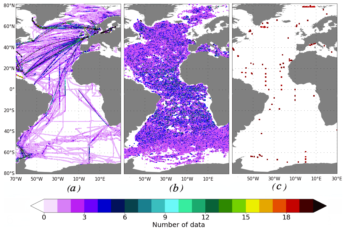
Figure 1 Spatial distribution of datasets used for training (number of measurements per grid point and 5 d time step): (a) SOCAT data for the period 2001–2010, (b) synthetic Argo data for the period 2008–2010, and (c) mooring positions modelled for the period 2008–2010.

2.1.2 Model output and pseudo-observations

Here we used the numerical output from an online-coupled physical–biogeochemical global ocean model, the Nucleus for European Modelling of the Ocean (NEMO)/PISCES model, at 5 d resolution. This configuration of the NEMO framework was implemented on a global tripolar grid. It coupled the ocean general circulation model OPA9 (Madec et al., 1998), the sea ice code LIM2 (Fichefet and Maqueda, 1997) and the biogeochemical model PISCESv1 (Aumont and Bopp, 2006). Information on the simulation is given in Gehlen et al. (2020) and Terhaar et al. (2019), including the evaluation of the modelled mean state and the seasonal cycle of sea surface temperature and sea–air fluxes of CO₂ (Gehlen et al., 2020). The geographical and time positions identified from the data mentioned before were used to create pseudo-observations by sub-sampling NEMO/PISCES model output at sites of real-world observations. Thus, the positions of SOCAT, Argo floats and mooring stations were chosen over 5 d centred on the NEMO/PISCES date and sub-sampled on the model grid. The model grid coordinate closest to the real geographical position was chosen. If several measurements were co-localised at the same grid coordinate and same time step, it is counted as one measurement. No Argo floats were added to grid cells if there was already a measurement identified in the SOCAT database. All predictors and target pCO₂ were taken from model output at corresponding coordinates. These outputs served as the reference for validation and evaluation of our experiments and for assessing the ML method's accuracy. The simulation covers the period 1958 to 2010; the last 3 years were retained for the design study.

2.2 Observational system simulation experiences

Table 1 summarises experiments designed for different combinations of observing platforms.

Table 1 Information on Observation System Simulation Experiments.

The first test is based on individual sampling data extracted from the SOCAT database. As mentioned before, these data provide a good coverage of the Northern Hemisphere. The lesser coverage in the Southern Hemisphere results in a larger dispersion of methods based on these observations only (Denvil-Sommer et al., 2019; Rödenbeck et al., 2015). This has motivated experiments with additional data from Argo profilers limited to the Southern Hemisphere. An experiment based on the full physical ARGO network was included to evaluate the method for a high spatial and temporal coverage (an optimal, yet unrealistic case).

We have tested combinations of SOCAT data and (1) total Argo data, (2) Argo only in the Southern Hemisphere, and (3) 25 % or (4) 10 % of the initial (total) Argo distribution. Finally, these experiments were repeated with additional mooring data. It is worth noting (Table 1) that OSSE 4 is closest to the target of the BioGeoChemical (BGC)-Argo program, with a BGC-Argo density corresponding to 25 % of the existing Argo distribution. However, we decided to choose OSSE 3 as a benchmark against which to evaluate individual experiments. This experiment has a high data density and provides additional information on a potential future BGC-Argo network.

2.3 Method

We used a feed-forward neural network (FFNN) based on Denvil-Sommer et al. (2019) to reconstruct surface ocean pCO₂ over the Atlantic Ocean. Compared to the previous study, we skipped the first step consisting of the reconstruction of the pCO₂ climatology. The reconstruction covered January 2008 to December 2010 with a 5 d frequency and at the spatial resolution of the tripolar ORCA025 model grid (nominal 0.25^∘ resolution). The approach consisted of a method that reconstructs the non-linear relationships between the target pCO₂ and predictors responsible for pCO₂ variability:

$$\begin{array}{}\text{(1)}& \begin{array}{rl}p{\mathrm{CO}}_{\mathrm{2},n}& =f({\mathrm{SSS}}_n,{\mathrm{SST}}_n{\mathrm{SSH}}_n,{\mathrm{Chl}}_n,{\mathrm{MLD}}_n,\\ & p{\mathrm{CO}}_{\mathrm{2},\mathrm{atm},n},{\mathrm{SSS}}_{\mathrm{anom},n},{\mathrm{SST}}_{\mathrm{anom},n},\\ & {\mathrm{SSH}}_{\mathrm{anom},n},{\mathrm{Chl}}_{\mathrm{anom},n},{\mathrm{MLD}}_{\mathrm{anom},n},\\ & p{\mathrm{CO}}_{\mathrm{2},\mathrm{atm},\mathrm{anom},n},{\mathrm{lat}}_n,{\mathrm{long}}_{\mathrm{1},n},{\mathrm{long}}_{\mathrm{2},n}).\end{array}\end{array}$$

As in Denvil-Sommer et al. (2019), we use Keras, a high-level neural network Python library (Chollet, 2015; https://keras.io, last access: 28 July 2021) to construct and train the FFNN models. We first identified an optimal configuration (number and size of hidden layers, the activation functions, etc.) of the FFNN model. Based on our earlier work (Denvil-Sommer et al., 2019), a hyperbolic tangent was chosen as an activation function for neurons in hidden layers, and a linear function was chosen for the output layer. As an optimisation algorithm, the mini-batch gradient descent or “RMSprop” was used (adaptive learning rates for each weight, Chollet, 2015; Hinton et al., 2012).

The numbers of hidden layers and parameters/weights depend on the number of data used for training. In this work, the FFNN was applied separately for each month (one model for January, one model for February, etc.). A sub-set of 50 % of data was used for training. A total of 25 % participated in the evaluation of the model during the training algorithm, and 25 % were used to validate the model after training. These data were chosen regularly in time and space: every third grid point was kept for evaluation, and every fourth grid point was kept for validation. Tables S1 in the Supplement presents the numbers of training data for each month and each OSSE. To adjust the number of FFNN parameters/weights we followed the empirical rule that suggests limiting the number of parameters to the number of training data points divided by 10 to avoid overfitting (Amari et al., 1997). The FFNNs for all OSSEs except OSSE 2 have four layers (two hidden layers) with 1116 parameters in total. The input layer has 15 input nodes and 20 output nodes that represent the input for the first hidden layer. The first hidden layer has 25 output nodes, and the second hidden layer has 10 output nodes. The OSSE 2, which is based on Argo data for the period 2008–2010, has significantly fewer data for training, and thus the FFNN for the OSSE 2 is different: three layers (one hidden layer with 20 input and 10 output nodes) with 541 total parameters.

All data have to be normalised before their use in the FFNN, as exemplified for SSS:

$$\begin{array}{}\text{(2)}& {\mathrm{SSS}}_n={\displaystyle \frac{\mathrm{SSS}-\stackrel{\mathrm{‾}}{\mathrm{SSS}}}{\mathrm{SD}\left(\mathrm{SSS}\right)}}.\end{array}$$

$\stackrel{\mathrm{‾}}{\mathrm{SSS}}$ is the total mean of variable SSS, and SD(SSS) is standard deviation of SSS.

Normalisation is required to rank all predictors on the same scale and to avoid the possible influence of one predictor with strong variability (Kallache et al., 2011).

Following Denvil-Sommer et al. (2019) we normalised the geographical positions (lat, long) in the following way:

$$\begin{array}{c}{\displaystyle }{\mathrm{lat}}_n=\sin (\mathrm{lat}\cdot \mathit{\pi }/\mathrm{180}),\\ {\displaystyle }{\mathrm{long}}_{n,\mathrm{1}}=\sin (\mathrm{long}\cdot \mathit{\pi }/\mathrm{180}),\\ {\displaystyle }{\mathrm{long}}_{n,\mathrm{2}}=\cos (\mathrm{long}\cdot \mathit{\pi }/\mathrm{180}).\end{array}$$

A K-fold cross-validation was used to evaluate and validate the FFNN architecture. The cross-validation is based on K=4 different subsamples where 25 % of independent data are chosen for validation. In each of the four cases, 25 % of the data are different and there is no overlap. Thereby, each run has four outputs. Different architectures of the FFNN were tested and the final one was chosen based on skill assessed by the root-mean-square difference (RMSD), the r² and the bias of four outputs for each architecture. To ensure a good accuracy of the method and check that there is no overfitting, we compared the RMSD, r² and bias estimated from the validation dataset with those estimated from the training dataset. Denvil-Sommer et al. (2019) provide a detailed description of the model, including the accuracy of the ML method and its ability to correctly reproduce the pCO₂ variability.

2.4 Diagnostics

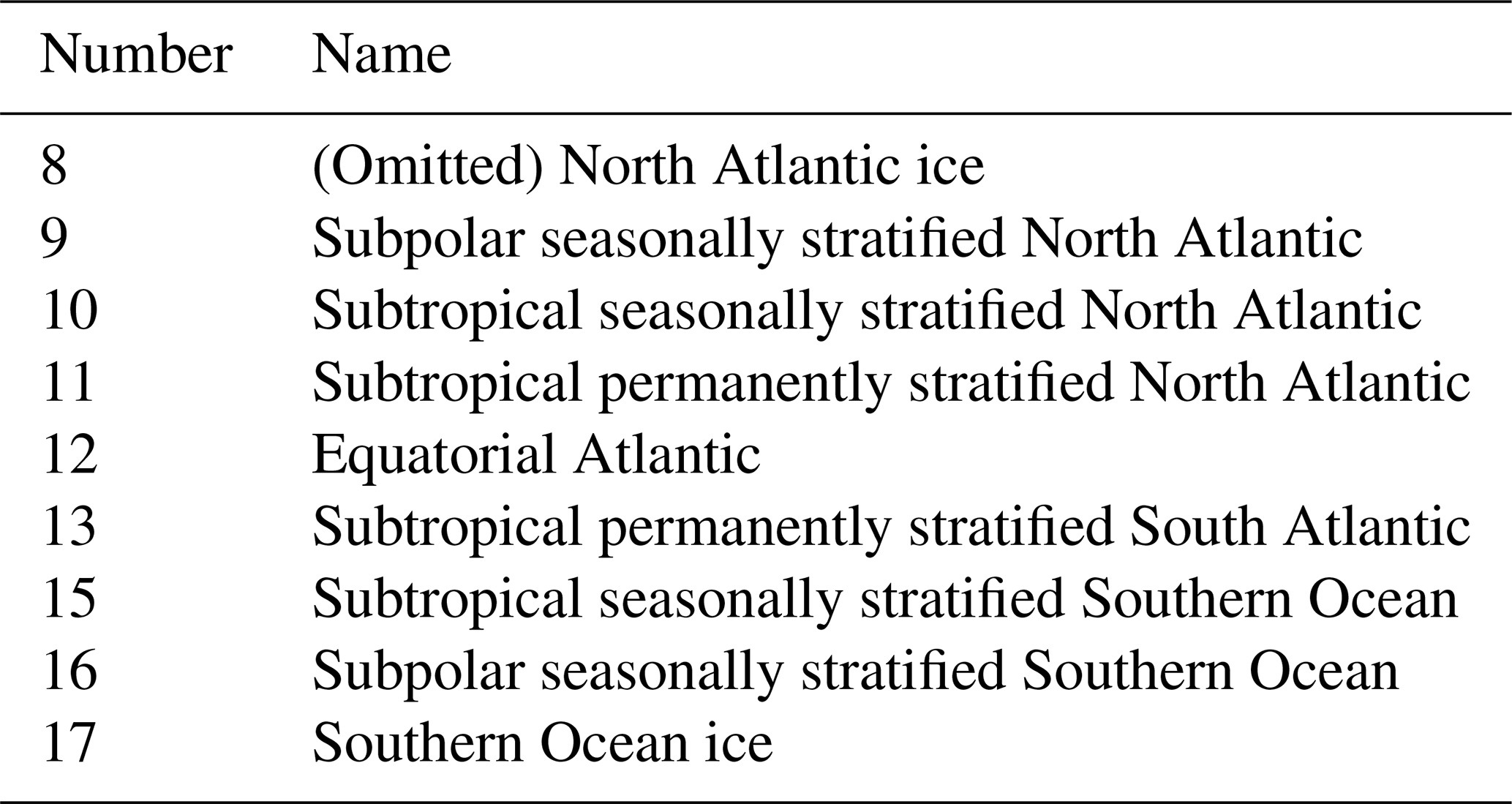
The comparison between OSSEs is done per biome, following Rödenbeck et al. (2015) (Fig. 2, Table 2). Biome 8, North Atlantic ice, has been omitted due to poor data coverage in all OSSEs. It is expected that reconstructions over this region will yield large biases susceptible to interfere with the interpretation of results from individual OSSEs.

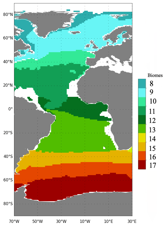
Figure 2 Map of biomes (following Rödenbeck et al., 2015; Fay and McKinley, 2014) focused on the region 70^∘ W–30^∘ E and used for comparison between OSSEs.

Table 2 Biomes from Fay and McKinley (2014) used for time series comparison (Fig. 2).

In order to simplify the comparison, we used Taylor and target diagrams with standard deviation, biases, correlation and normalised RMSD (uRMSD) of the mean of four FFNN outputs for each OSSE. Here uRMSD is estimated as follows:

$$\begin{array}{}\text{(3)}& \begin{array}{rl}\mathrm{uRMSD}=& \sqrt{\mathrm{mean}\left(\mathit{\right\{}[p{\mathrm{CO}}_{\mathrm{2}\mathrm{OSSE}}-\stackrel{\mathrm{‾}}{p{\mathrm{CO}}_{\mathrm{2}\mathrm{OSSE}}}]}\\ & \stackrel{\mathrm{‾}}{-[p{\mathrm{CO}}_{\mathrm{2}\mathrm{NEMO}}-\stackrel{\mathrm{‾}}{p{\mathrm{CO}}_{\mathrm{2}\mathrm{NEMO}}}]{\mathit{\}}}^{\mathrm{2}})}.\end{array}\end{array}$$

For each OSSE and each output of the k-fold cross-validation, we estimated a time mean difference between its pCO₂ and NEMO pCO₂ at each grid point:

$$\begin{array}{rl}{\mathrm{Diff}}_{j,i}& ={\mathrm{mean}}_T(p{\mathrm{CO}}_{\mathrm{2}\mathrm{OSSE}j,i}-p{\mathrm{CO}}_{\mathrm{2}\mathrm{NEMO}})\\ & ={\displaystyle \frac{\mathrm{1}}{T}}\sum _{t=\mathrm{1}}^T(p{\mathrm{CO}}_{\mathrm{2}\mathrm{OSSE}j,i,t}-p{\mathrm{CO}}_{\mathrm{2}\mathrm{NEMO}t}),\end{array}$$

where mean_T is a time mean over the period, T is a number of time steps, j is an index of the OSSE and i is an index of output from 1 to 4.

Further, the maximum absolute value from four outputs, maxValue_j, was estimated for each OSSE:

$${\mathrm{maxValue}}_j={\max }_i\left(\mathrm{abs}\right({\mathrm{Diff}}_{j,i}\left)\right),$$

where max_i is a maximum value on i, the index of output, for each fixed j, i.e. the OSSE index. The index i of the maximum absolute value of FFNN outputs is called i_max.

The final mean difference meanD_j was estimated as follows:

$$\begin{array}{}\text{(4)}& {\mathrm{meanD}}_j=\mathrm{sign}\left({\mathrm{Diff}}_{j,i_{max}}\right)\cdot {\mathrm{maxValue}}_j,\end{array}$$

where sign(x) is a function that returns the sign of a value x, either −1 or 1.

The SD of the mean difference Diff_j,i is estimated for each OSSE as follows:

$$\begin{array}{}\text{(5)}& {\mathrm{SD}}_j=\mathrm{SD}\left({\mathrm{Diff}}_{j,i}\right),\end{array}$$

where j is fixed and all outputs of FFNN i are included in the estimation of SD.

The time series of the mean value from four FFNN outputs for pCO₂ were provided per biome, with the maximum and minimum values from these four outputs indicated by shading. The time series of CO₂ sea–air flux are shown in the same way as the ones for pCO₂. The sea–air CO₂ flux, fgCO₂, was calculated following Rödenbeck et al. (2015):

$$\begin{array}{}\text{(6)}& \mathit{fg}{\mathrm{CO}}_{\mathrm{2}}=k\mathit{\rho }L(p{\mathrm{CO}}_{\mathrm{2}}-p{\mathrm{CO}}_{\mathrm{2},\mathrm{atm}}),\end{array}$$

ρ is seawater density and L is the temperature-dependent solubility (Weiss, 1974). k is the piston velocity estimated as follows (Wanninkhof, 1992):

$$k=\mathrm{\Gamma }{u}^{\mathrm{2}}({\mathit{Sc}}^{{\mathrm{CO}}_{\mathrm{2}}}/{\mathit{Sc}}^{\mathrm{ref}}{)}^{-\mathrm{0.5}}.$$

The global scaling factor Γ was estimated following Rödenbeck et al. (2014) with the global mean CO₂ piston velocity equaling 16.5 cm h⁻¹. Sc corresponds to the Schmidt number estimated according to Wanninkhof (1992). The wind speed was computed from 6-hourly NCEP wind speed data (Kalnay et al., 1996). To simplify the interpretation of results, the NEMO/PISCES CO₂ sea–air flux was also calculated by using Eq. (4) and NCEP wind speed.

3 Results

Figure 3 shows the Taylor diagram (correlation coefficient between reconstructed pCO₂ and model output and standard deviation of reconstructed fields) of 11 OSSEs in the region of eight biomes (pink) and in each of these biomes separately (colour code corresponds to Fig. 2). The target diagrams per biome for each OSSE are presented on Fig. 4. Over regions well covered with observations (biomes 9, 10, 11), results of different OSSEs lie close to each other. The OSSE 1 (marker symbol “+”; Fig. 3a) that is based only on SOCAT data has a lower correlation coefficient over the whole region (0.67, pink) and per biome (Fig. 3a). Over regions with poor observational coverage the results from OSSE 1 lie at a distance from results of all other OSSEs. OSSE 1 also shows the largest uRMSDs (Fig. 4), as exemplified for biome 17 with uRMSD of 17.33 µatm, SD of 21.11 µatm (compared to 24.03 µatm estimated from NEMO/PISCES data) and bias of −11.63 µatm (all values in the Figs. 3 and 4 are presented in Tables 3 and 4). The OSSE 2 (based on all Argo data, “O”) and OSSE 3 (combination of Argo and SOCAT data, “X”) provide comparable results (Fig. 3b and c). OSSE 3 tends to have a smaller uRMSD and bias and lies closer to the SD values from the NEMO/PISCES model (Fig. 4). OSSE 3 is based on the maximum of pseudo-observations for training and most likely represents an unrealistic endmember. However, as mentioned before, OSSE 3 is used as the benchmark to find other OSSEs with similar results and more feasible data coverage.

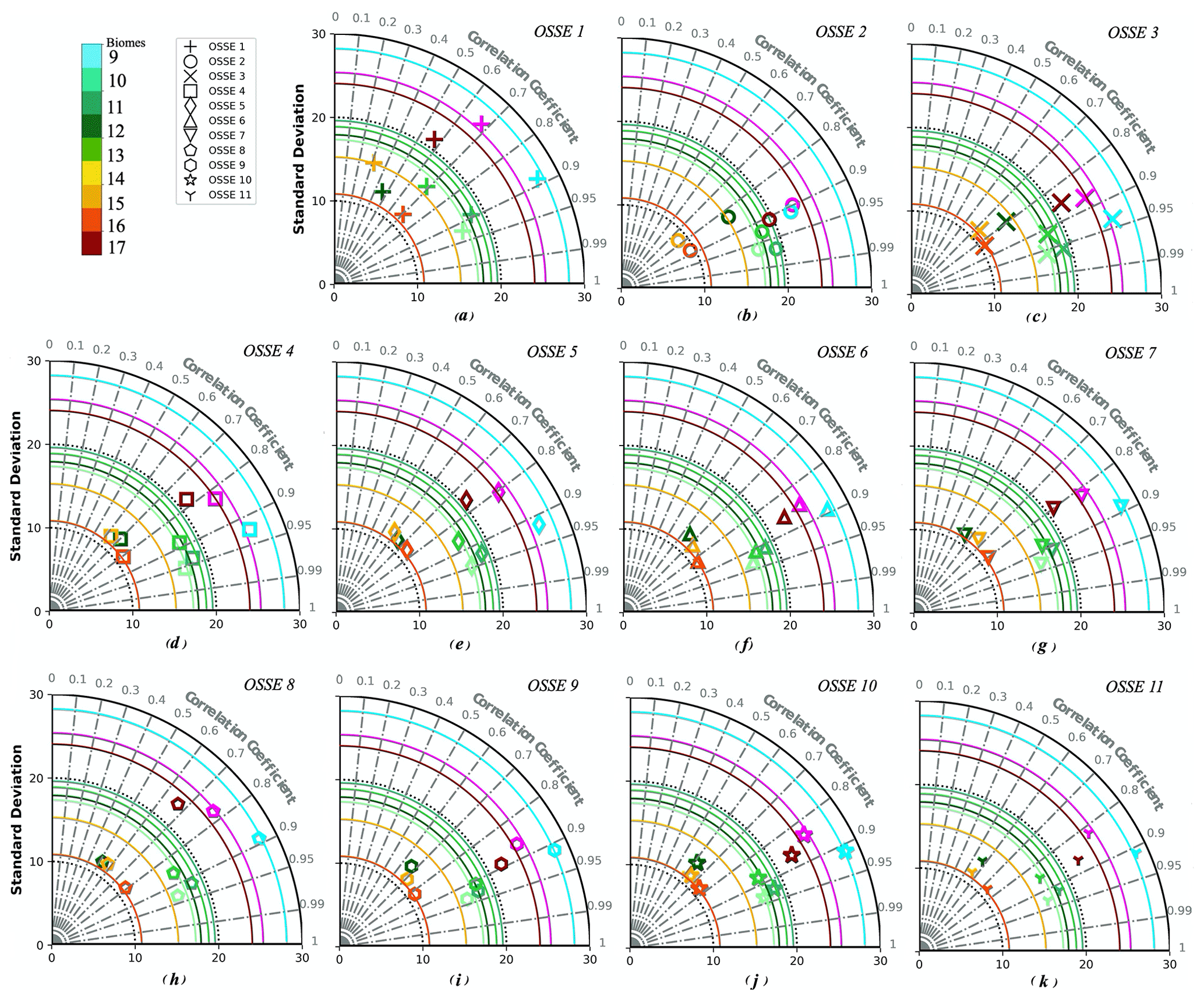
Figure 3 Taylor diagram of 11 OSSEs summarised in Table 2; the colour code corresponds to Fig. 2, and the purple colour represents all of the eight biomes combined: (a) OSSE 1, which uses SOCAT data only; (b) OSSE 2, which uses synthetic Argo data only; (c) OSSE 3, which uses SOCAT and synthetic Argo data; (d) OSSE 4, which uses SOCAT data and 25 % of the original synthetic Argo data; (e) OSSE 5, which uses SOCAT data and 10 % of the original synthetic Argo data; (f) OSSE 6, which uses SOCAT data and synthetic Argo data in the Southern Hemisphere; (g) OSSE 7, which uses SOCAT data and 25 % of the original synthetic Argo data in the Southern Hemisphere; (h) OSSE 8, which uses SOCAT data and 10 % of the original synthetic Argo data in the Southern Hemisphere; (i) OSSE 9, which uses SOCAT data, synthetic Argo data in the Southern Hemisphere, and data from mooring stations; (j) OSSE 10, which uses SOCAT data, 25 % of the original synthetic Argo data in the Southern Hemisphere, and data from mooring stations; and (k) OSSE 11, which uses SOCAT data, 10 % of the original synthetic Argo data in the Southern Hemisphere, and data from mooring stations.

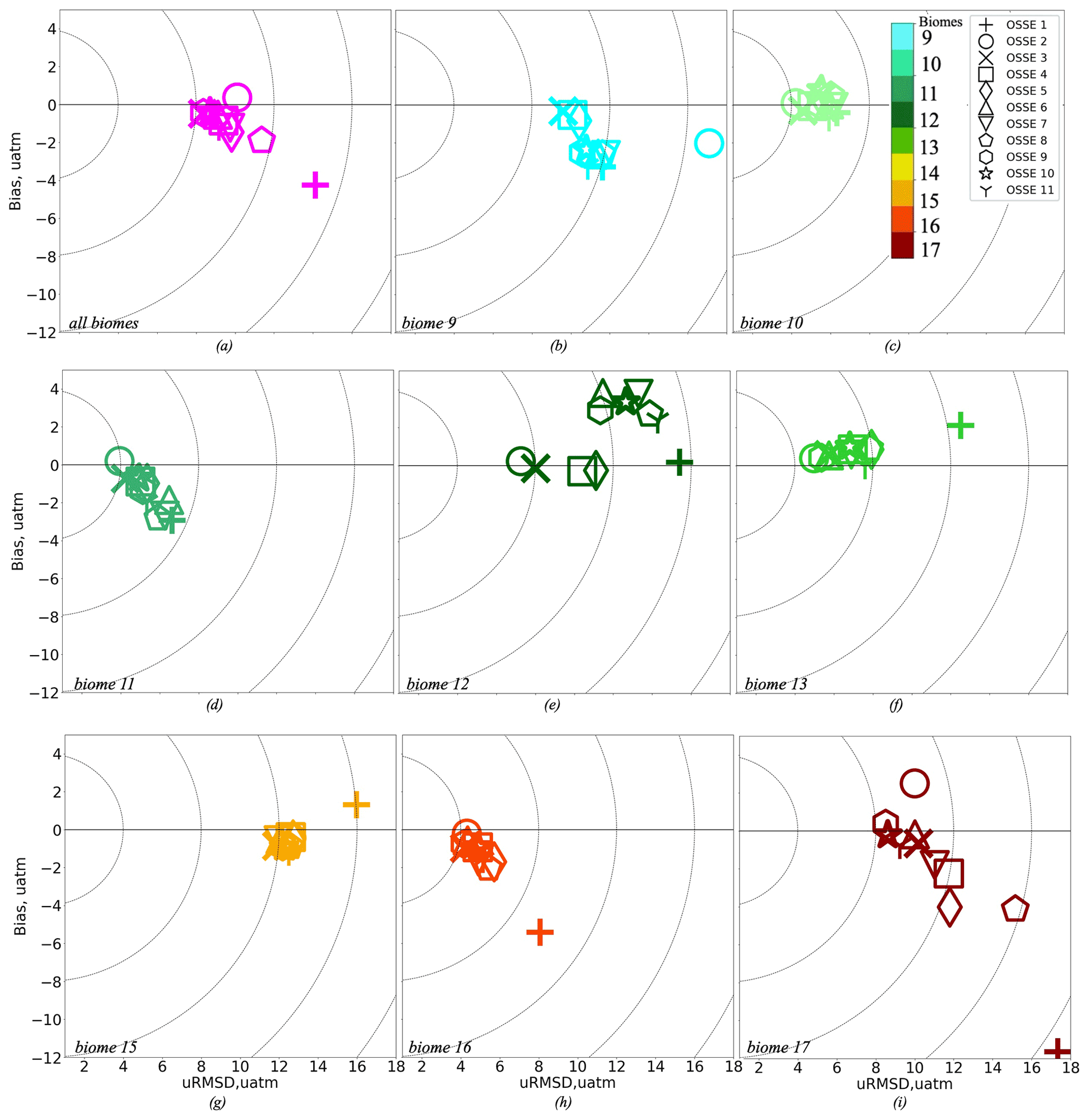
Figure 4 Target diagram per biome for 11 OSSEs, the colour code corresponds to Fig. 2, and the purple colour represents all of the eight biomes combined: (a) all eight biomes, (b) biome 9 (subpolar seasonally stratified North Atlantic), (c) biome 10 (subtropical seasonally stratified North Atlantic), (d) biome 11 (subtropical permanently stratified North Atlantic), (e) biome 12 (equatorial Atlantic), (f) biome 13 (subtropical permanently stratified South Atlantic), (g) biome 15 (subtropical seasonally stratified Southern Ocean), (h) biome 16 (subpolar seasonally stratified Southern Ocean), (i) biome 17 (Southern Ocean ice). OSSE 1 uses SOCAT data only; OSSE 2 uses synthetic Argo data only; OSSE 3 uses SOCAT and synthetic Argo data; OSSE 4 is SOCAT data and 25 % of the original synthetic Argo data; OSSE 5 uses SOCAT data and 10 % of the original synthetic Argo data; OSSE 6 uses SOCAT data and synthetic Argo data in the Southern Hemisphere; OSSE 7 uses SOCAT data and 25 % of the original synthetic Argo data in the Southern Hemisphere; OSSE 8 uses SOCAT data and 10 % of the original synthetic Argo data in the Southern Hemisphere; OSSE 9 uses SOCAT data, synthetic Argo data in the Southern Hemisphere, and data from mooring stations; OSSE 10 uses SOCAT data, 25 % of the original synthetic Argo data in the Southern Hemisphere, and data from mooring stations; and OSSE 11 uses SOCAT data, 10 % of the original synthetic Argo data in the Southern Hemisphere, and data from mooring stations. OSSEs 1, 3 and 10 are in bold as we focus our detailed comparison on these three OSSEs.

Table 3 Correlation coefficient and standard deviation (µatm) of 11 OSSEs from Table 2 estimated over eight Atlantic Ocean biomes and at basin scale; the results are presented in Fig. 3. OSSEs 1, 3 and 10 are in bold as we focus our detailed comparison on these three OSSEs.

Table 4 Normalised root-mean-square differences and biases (µatm) of 11 OSSEs from Table 2 estimated over eight Atlantic Ocean biomes and at basin scale; the results are presented in Fig. 4. OSSEs 1, 3 and 10 are in bold as we focus our detailed comparison on these three OSSEs.

OSSE 4 (square) and OSSE 5 (rhombus) are based on OSSE 3, the only difference being the percentage of Argo data used: OSSE 3 uses 100 %, OSSE 4 uses 25 % and OSSE 5 uses 10 %. The results of OSSEs 4 and 5 are similar to those obtained for OSSE 3. The largest difference is observed over biome 17 (Figs. 3, 4i): correlation coefficients are 0.85 (OSSE 3), 0.77 (OSSE 4), and 0.75 (OSSE 5); biases are −0.66, −2.25, and −4.02 µatm; and uRMSDs are 10.18, 11.75, and 11.8 µatm (Tables 3, 4).

OSSEs 6 (triangle), 7 (inverted triangle), and 8 (pentahedron) were trained on SOCAT data complemented with Argo data in the Southern Hemisphere. In general, the skill scores are lower compared to OSSE 3, especially for OSSE 8 (10 % of Argo data in the Southern Hemisphere) where results approach those of OSSE 1 (Fig. 3). Large differences are obtained for biomes 12 and 17 (Figs. 3, 4e and i): in biome 12 (17), correlation coefficients for OSSE 6, 7, 8 are 0.64 (0.86), 0.54 (0.8), and 0.52 (0.66) compared to 0.79 (0.85) for OSSE 3; uRMSDs are 11.46 (10.01), 13.3 (11.03), and 13.87 (15.16) µatm compared to 8 (10.18) µatm for OSSE 3; and biases are 3.82 (−0.18), 3.77 (−1.8), and 2.7 (−4.12) µatm compared to −0.14 (−0.66) µatm for OSSE 3 (Tables 3, 4). Over biome 12 all OSSEs show SD values lower than the one computed for NEMO/PISCES model output (Table 3). This could result from the SD of the mean output being slightly lower than the individual SDs for four OSSE FFNN outputs (not shown). However, individual SDs also underestimate the NEMO/PISCES SD, which might suggest that the ensemble of predictors does not properly represent the variability over the equatorial Atlantic.

Table 5 Differences (Eq. 4) between OSSE FFNN outputs and NEMO/PISCES pCO₂ and its standard deviation (SD) (Eq. 5) (in µatm).

Reconstruction skill scores are improved by the addition of data from mooring stations to OSSEs 6, 7 and 8 in OSSEs 9 (hexagon), 10 (star) and 11 (triangle centroid) (Fig. 3 and 4, Tables 3 and 4). Over the ensemble of eight biomes the decrease in the number of Argo data goes along with a general decrease of correlation coefficients, i.e. 0.88 (OSSE 9), 0.85 (OSSE 10), 0.83 (OSSE 11), and an increase of uRMSDs, i.e. 8.37 µatm (OSSE 9), 8.71 µatm (OSSE 10), 9.16 µatm (OSSE 11) (Figs. 3, 4a, Tables 3 and 4). Statistics are slightly worse for OSSE 11 compared to OSSEs 9 and 10, which have comparable results. While OSSE 10 shows a smaller correlation coefficient over the whole region compared to OSSE 9, its SD (24.89 µatm) lies closer to the NEMO/PISCES SD (25.34 µatm), and it has a smaller bias (−0.39 µatm). Similar results are found over other biomes: in biome 12, OSSEs 9 and 10 have correlation coefficients close to each other (0.68 and 0.63, respectively) and larger than for OSSEs 6, 7 and 8, while for OSSE 11 it is 0.58. The SDs are almost equal (OSSE 9: 12.98 µatm; OSSE 10: 12.9 µatm), and the uRMSDs have a small difference compared to the one computed for OSSE 3 (8 µatm) (Tables 3, 4). Thus, the remainder of the discussion will focus on OSSE 10 in comparison to OSSEs 1 and 3. OSSE 10 provides comparable results to OSSE 9 and is in good agreement with OSSE 3 while using a lower percentage of data for training. Figures 3 and 4 are summarised in Fig. S1 of the Supplement.

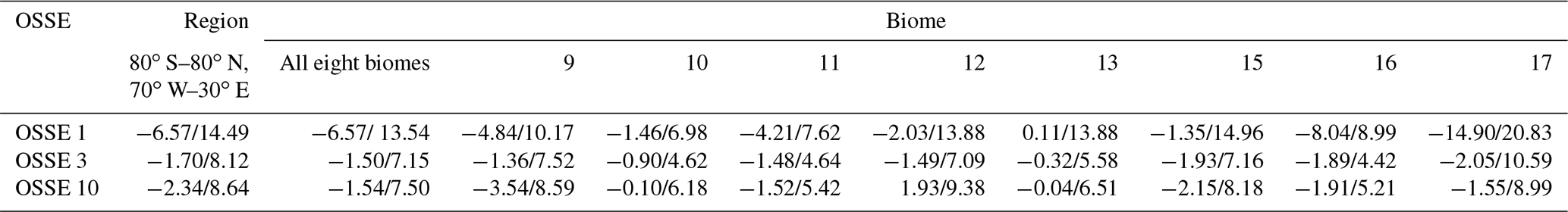
Figure 5a, b and c present the differences between reconstructed pCO₂ distributions (Fig. 5a – OSSE 1; Fig. 5b – OSSE 3; Fig. 5c – OSSE 10) and NEMO/PISCES output. The maximum in absolute value from four outputs for each OSSE FFNN is shown (Eq. 4). There is a large improvement in the Southern Hemisphere for OSSEs 3 (Fig. 5b) and 10 (Fig. 5c) compared to OSSE 1 (Fig. 5a): the difference varies mostly between −3 and 3 µatm for OSSEs 3 and 10, and between −15 and 15 µatm for OSSE 1 (Fig. 5). However, the average values of the mean over biomes are not always better for OSSE 3 (Table 5): in biome 13, OSSE 1 shows a small positive difference of 0.11 µatm, while for OSSE 3 a negative difference of −0.32 µatm is computed, exceeding 0.11 µatm in its absolute value. This is due to error compensation by averaging; the reduction of the positive difference in the middle of biome 13 in OSSE 3 increases the impact of negative small differences in this region. Error compensation also contributes to positive biases computed for OSSEs 6–11 for biome 12 (Table 4). Additional data from Argo floats correct the negative bias in the southern part of the biome close to the African coast (Fig. 5c). Thus, the strong positive bias in the northern part becomes dominant and results in a total positive bias. A large improvement is obtained in biomes 16 and 17: from −8.04 µatm for OSSE 1 to −1.89 and −1.91 µatm for OSSEs 3 and 10 in biome 16, respectively, and from −14.9 µatm for OSSE 1 to −2.05 and −1.55 µatm for OSSEs 3 and 10, respectively, in biome 17 (Table 5). Over the whole region (80^∘ S–80^∘ N, 70^∘ W–30^∘ E), OSSE 1 has a mean difference of −6.57 µatm, it is −1.7 and −2.34 µatm for OSSEs 3 and 10. The difference between OSSEs 3 and 10 results from the Labrador Sea and Baffin Bay: OSSE 10 has fewer data in this region compared to the OSSE 3. However, there is an improvement in OSSE 10 compared to OSSE 1 and 3 in the Greenland Sea (Fig. 5). It results from the addition of mooring data in the Greenland Sea region (Fig. 1c).

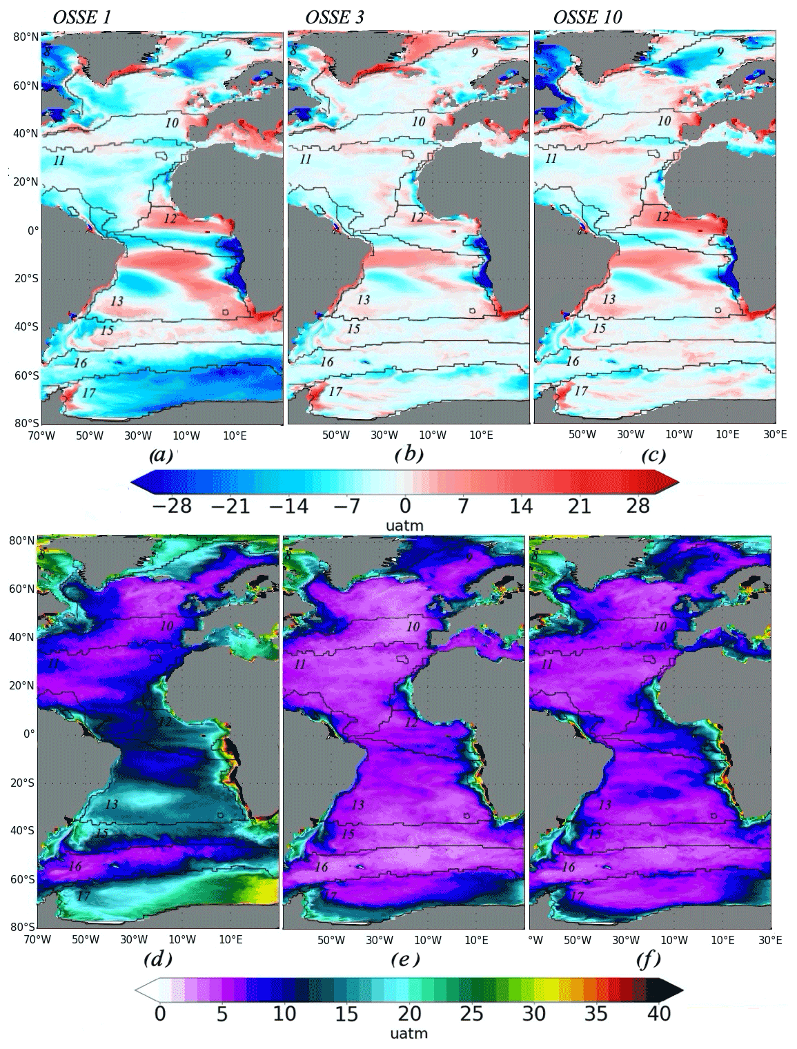
Figure 5 Differences between OSSE FFNN outputs and NEMO/PISCES pCO₂ and its standard deviation (SD; in µatm): (a, b, c) its maximum and minimum values from four outputs for each OSSE FFNN (Eq. 4) and (g, h) standard deviation of differences for all four outputs for each OSSE FFNN (Eq. 5). (a, d) OSSE 1 using SOCAT data only; (b, e) OSSE 3 using SOCAT and synthetic Argo data; and (c, f) OSSE 10 using SOCAT data, 25 % of the original synthetic Argo data in the Southern Hemisphere, and data from mooring stations. Contours and numbers on maps correspond to biomes.

Figure 5d, e and f present the standard deviations (SD) of differences for all four outputs for each OSSE FFNN (Fig. 5d – OSSE 1; Fig. 5e – OSSE 3; Fig. 5f – OSSE 10) (Eq. 5). Over most of the Atlantic Ocean, SD varies between 0 and 10 µatm for OSSEs 3 and 10. In each case there is a strong SD along the coasts and in the Labrador Sea and Baffin Bay. In general, the mean value of SD tends to decrease (Table 5) from OSSE 1 to OSSEs 3 and 10. In the Southern Hemisphere SD reaches up to 30 µatm (Fig. 5d, e and f) when only SOCAT data are used in the FFNN algorithm (OSSE 1). It is significantly reduced in response to the addition of float data in OSSEs 3 and 10, which also show less spatial variability. The results for other OSSEs are added to the Supplement (Table S2, Figs. S2, S3).

Figure 6 shows the correlation between the mean value of four OSSE outputs and NEMO/PISCES pCO₂ (Fig. 6a – OSSE 1; Fig. 6b – OSSE 3; Fig. 6c – OSSE 10). The additional data from Argo floats and mooring stations increase the correlation coefficient from 0.68 in the case of OSSE 1 (SOCAT data only) to 0.86 and 0.85 in the case of OSSEs 3 and 10 (Table 6). A higher correlation was also obtained for these two OSSEs compared to OSSE 1 over the region covering the Greenland Sea, the Norwegian Sea and Barents Sea (mostly biome 9). In the Southern Hemisphere the correlation with NEMO/PISCES pCO₂ is also larger when Argo data are included, especially in biomes 16 and 17: 0.7 and 0.57 for OSSE 1, 0.83 and 0.85 for OSSE 3, and 0.78 and 0.89 for OSSE 10 (Table 6). However, there is a low correlation along the African coasts, which is in agreement with our previous results for mean difference and SD (Fig. 5). It reflects the predominantly open-ocean data used for this exercise. A well-pronounced decrease in correlation is observed for biome 15 (subtropical seasonally stratified Southern Ocean). Such a decrease can result from the spatial distribution of data or from the predictor dataset. We will discuss it further in the next section. The results for other OSSEs are presented in the Supplement (Table S3, Fig. S4).

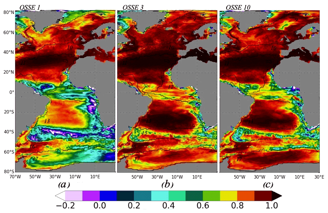
Figure 6 Correlation coefficient between OSSE FFNN outputs and NEMO/PISCES pCO₂: (a) OSSE 1 using SOCAT data only; (b) OSSE 3 using SOCAT and synthetic Argo data; and (c) OSSE 10 using SOCAT data, 25 % of the original synthetic Argo data in the Southern Hemisphere, and data from mooring stations. Contours and numbers on maps correspond to biomes.

Table 6 Correlation coefficient between OSSEs and NEMO/PISCES pCO₂.

In Fig. 7, time series of pCO₂ for OSSEs 1, 3 and 10 are compared to corresponding NEMO/PISCES model output. For each OSSE, the mean pCO₂ from four FFNN outputs is shown, as well as the mean bias (OSSE–NEMO/PISCES). Figure 7a and b presents the pCO₂ time series over the period of reconstruction 2008–2010 for OSSE 1, 3 and 10 compared to NEMO/PISCES pCO₂ used as reference (black) over all biomes. For OSSE 1 (SOCAT data only) a large difference and an underestimation of reconstructed pCO₂ (blue) compared to NEMO/PISCES pCO₂ (black) are found: the maximum error is up to −10 µatm (Fig. 7b). On the contrary, OSSEs 3 and 10 show a good agreement with NEMO/PISCES model output. Averages of pCO₂ over the eight biomes are 372.18 µatm for OSSE 3, 372.26 µatm for OSSE 10 and 368.39 µatm for OSSE 1, compared to 372.65 µatm for NEMO/PISCES (Table 7). The experiment corresponding to the BGC-Argo distribution target over the entire Atlantic basin, OSSE 4 (Figs. S8, S9), has a basin-wide average pCO₂ equal to 371.8 µatm (Table 7). This corresponds to a larger difference with NEMO/PISCES (−0.84 µatm) compared to OSSEs 3 and 10.

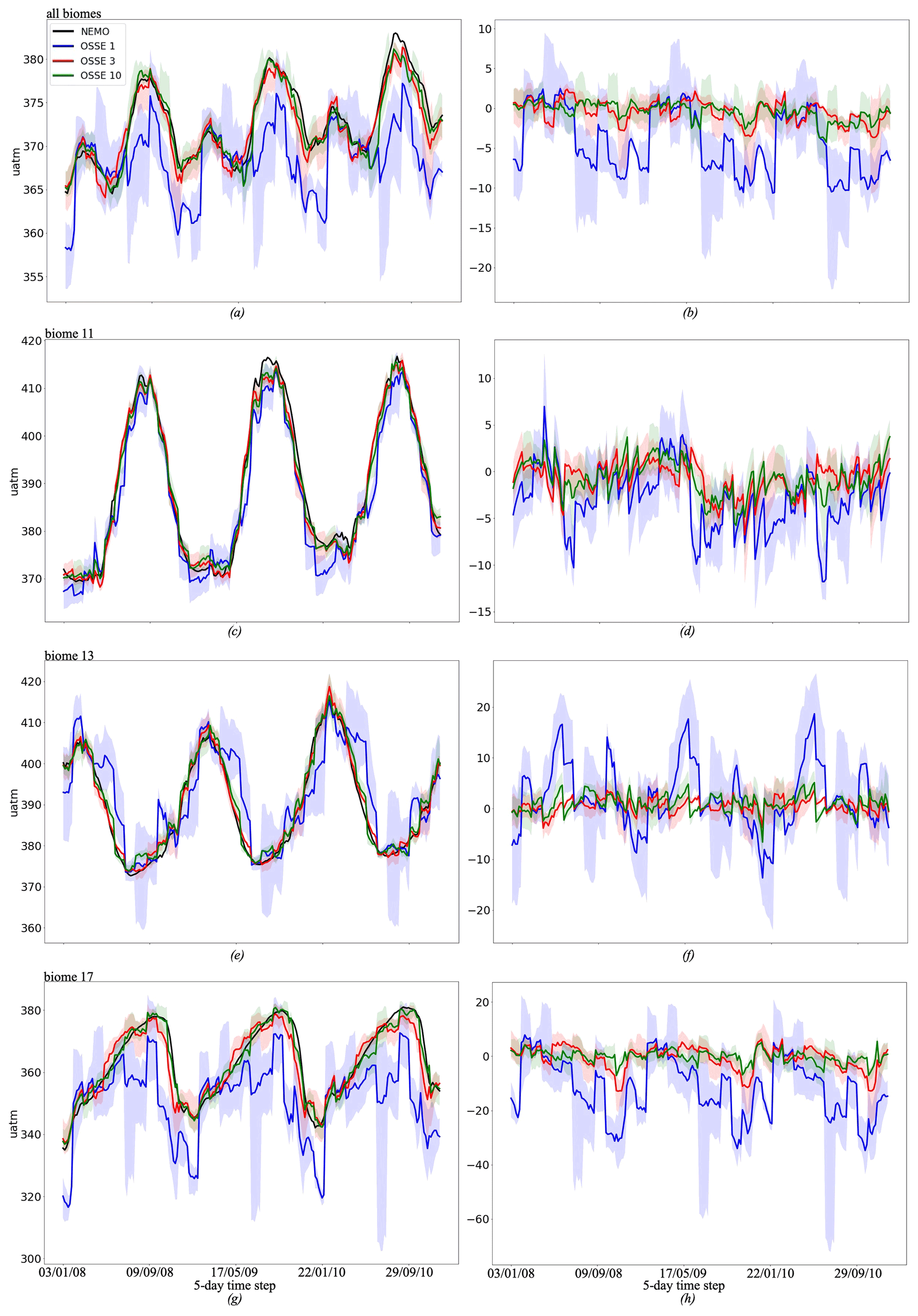
Figure 7 (a, c, e) Mean of four FFNN outputs for OSSE 1 (blue) (SOCAT data only), 3 (red) (SOCAT and synthetic Argo data), and 10 (green) (SOCAT data, 25 % of the original synthetic Argo data in the Southern Hemisphere, and data from mooring stations); shading corresponds to the maximum and minimum values from four FFNN outputs for each OSSE. The black curve shows NEMO/PISCES pCO₂. (b, d, f) Mean of differences of four FFNN outputs between OSSE 1 (blue), 3 (red), and 10 (green) and NEMO/PISCES pCO₂; shading corresponds to the maximum and minimum values of differences from four FFNN outputs for each OSSE. (a, b) Estimates are available over all biomes presented in Fig. 2, except biome 8: (c, d) biome 11 (subtropical permanently stratified North Atlantic), (e, f) biome 13 (subtropical permanently stratified South Atlantic), and (g, h) biome 17 (Southern Ocean ice).

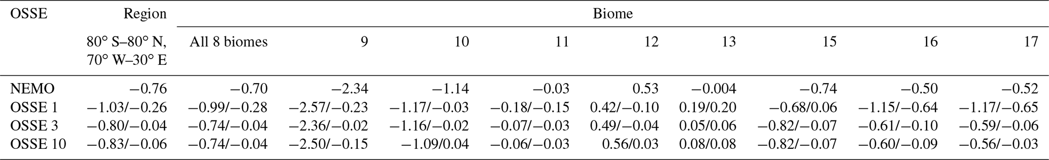
Table 7 pCO₂ averaged over the region (80^∘ S–80^∘ N, 70^∘ W–30^∘ E) and biomes from Fig. 2 for the NEMO/PISCES model; OSSEs 1, 3, and 10; and the corresponding averaged differences between OSSEs and NEMO/PISCES (in µatm).

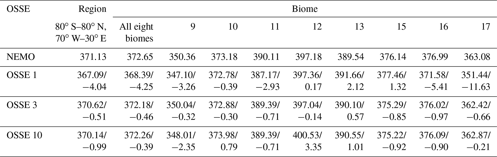
Figure 7c–h illustrate time series of reconstructed pCO₂ for biomes with varying data coverage. Biome 11, the subtropical permanently stratified North Atlantic (Fig. 7c and d), is well covered by data. All three OSSEs yield pCO₂ reconstructions that are in good accordance with the NEMO/PISCES reference. The amplitude and the phasing of the seasonal cycle are well reproduced. The bias varies within a range of ±5 µatm for OSSEs 3 and 10. A predominantly negative bias is found for OSSE 1 with values as high as −10 µatm. The pCO₂ averaged over biome 11 for OSSE 10 is close to NEMO/PISCES with, respectively 389.39 and 390.11 µatm (Table 7). OSSE 1 yields a biome-averaged pCO₂ equal to 387.11 µatm, while it is 389.39 µatm for the OSSE 3.

Biome 13, the subtropical permanently stratified South Atlantic (Fig. 7e and f), corresponds to a region with a low data coverage. This region has a dynamic similar to biome 11 in the Northern Hemisphere; however, the data coverage in biome 13 represents only 15 % of data coverage in biome 11 (Fig. S5). We observe a large difference between pCO₂ reconstructed by OSSE 1 (blue) and NEMO/PISCES (black). While the phasing of the reconstructed seasonal cycle is satisfying, it is noisy with a systematic overestimation in spring by up to 18 µatm (Table 7). However, the total averaged pCO₂ over biome 13 for OSSE 1 is close to the one of NEMO/PISCES: 391.66 µatm versus 389.54 µatm. The preceding suggests that while the variability of the predictors (mainly SST) is sufficient to constrain the biome-average pCO₂ and the phasing of the seasonal cycle at the first order, an improved coverage by in situ observations is needed for a smooth reconstruction of the seasonal cycle and its amplitude. Reconstructions are largely improved by the addition of data from Argo floats (OSSE 3) and moorings (OSSE 10). Biases mostly range between −3 and 3 µatm for these OSSEs.

The Southern Ocean ice biome (biome 17) is characterised by sparse data coverage and a bias towards the ice-free season. The results for biome 17 are presented in Fig. 7g and h. OSSE 1 underestimates the pCO₂ in this region over the full seasonal cycle. The maximum difference is obtained in September–October, which also corresponds to the months with the lowest number of available observations (Fig. S5). The biome-wide average is 351.44, −11.63 µatm below the NEMO/PISCES reference. The reconstruction is much improved for OSSEs 3 and 10 for the phasing and amplitude of the seasonal cycle and for the biome-wide averages. The averages are 362.42 and 362.87 µatm, respectively, for OSSE 3 and OSSE 10, compared to 363.08 µatm computed for NEMO/PISCES (Table 7).

Results for all OSSEs and for all biomes are included in the Supplement (Table S4, Figs. S6–S11).

Figure 8 shows the sea–air CO₂ flux time series (negative, uptake of CO₂ by the ocean). Over all biomes and in the region 80^∘ S–80^∘ N, 70^∘ W–30^∘ E, OSSEs 3 (red) and 10 (green) show a good agreement with NEMO/PISCES fgCO₂: the differences vary around zero and mostly do not exceed ±0.3 Pg yr⁻¹ (Fig. 8b, d, f and h). The total averaged fgCO₂ for OSSE 3 and 10 are −0.74 Pg yr⁻¹ compared to −0.7 Pg yr⁻¹ in NEMO/PISCES, while for OSSE 1 it equals −0.99 Pg yr⁻¹ (Table 8). The mean value over biome 11 is slightly better for OSSE 10 than for OSSE 3 compared to NEMO/PISCES: −0.06 Pg yr⁻¹ (OSSE 10), −0.07 (OSSE 3) and −0.03 Pg yr⁻¹ for NEMO/PISCES. The OSSE 1 (blue) shows again a large difference, it overestimates the ocean sink computed by the NEMO/PISCES model mostly during the whole period (Fig. 8b). In the well data-covered biome 11, OSSE 1 also has a tendency to overestimate the sea–air CO₂ flux (Fig. 8d): the total averaged fgCO₂ is −0.18 Pg yr⁻¹ for OSSE 1, while it is −0.03 Pg yr⁻¹ in the model. While the phasing and amplitude of the seasonal cycle of sea–air fluxes of CO₂ are well reproduced over biome 13 by OSSEs 3 and 10, the fgCO₂ reconstructed by OSSE 1 is noisy with differences with respect to the model reference of up 1 Pg yr⁻¹ (Fig. 8e). The maximum differences between OSSE 1 and NEMO/PISCES are systematically found in January and June, the months with the lowest number of available observations for training (Fig. S5). The biome-wide mean sea–air flux of CO₂ is close to zero in NEMO/PISCES: −0.004 Pg yr⁻¹. This slight uptake of CO₂ by the ocean in the model reference is not reproduced by the OSSEs that yield a source over biome 13, albeit of variable strength: 0.19 Pg yr⁻¹ for OSSE 1, 0.05 Pg yr⁻¹ for OSSE 3 and 0.08 Pg yr⁻¹ for OSSE 10. Over the Southern Ocean biome 17 (Fig. 8g and h), OSSE 1 (blue) overestimates fgCO₂ by −0.65 g yr⁻¹ (Table 8). OSSE 10 (green) reproduces the local maxima and minima of the fgCO₂ time series slightly better than OSSE 3, with average differences equaling −0.03 and −0.06 Pg yr⁻¹, respectively. Results for all OSSEs and for all biomes can be found in the Supplement (Table S5, Figs. S12–S17).

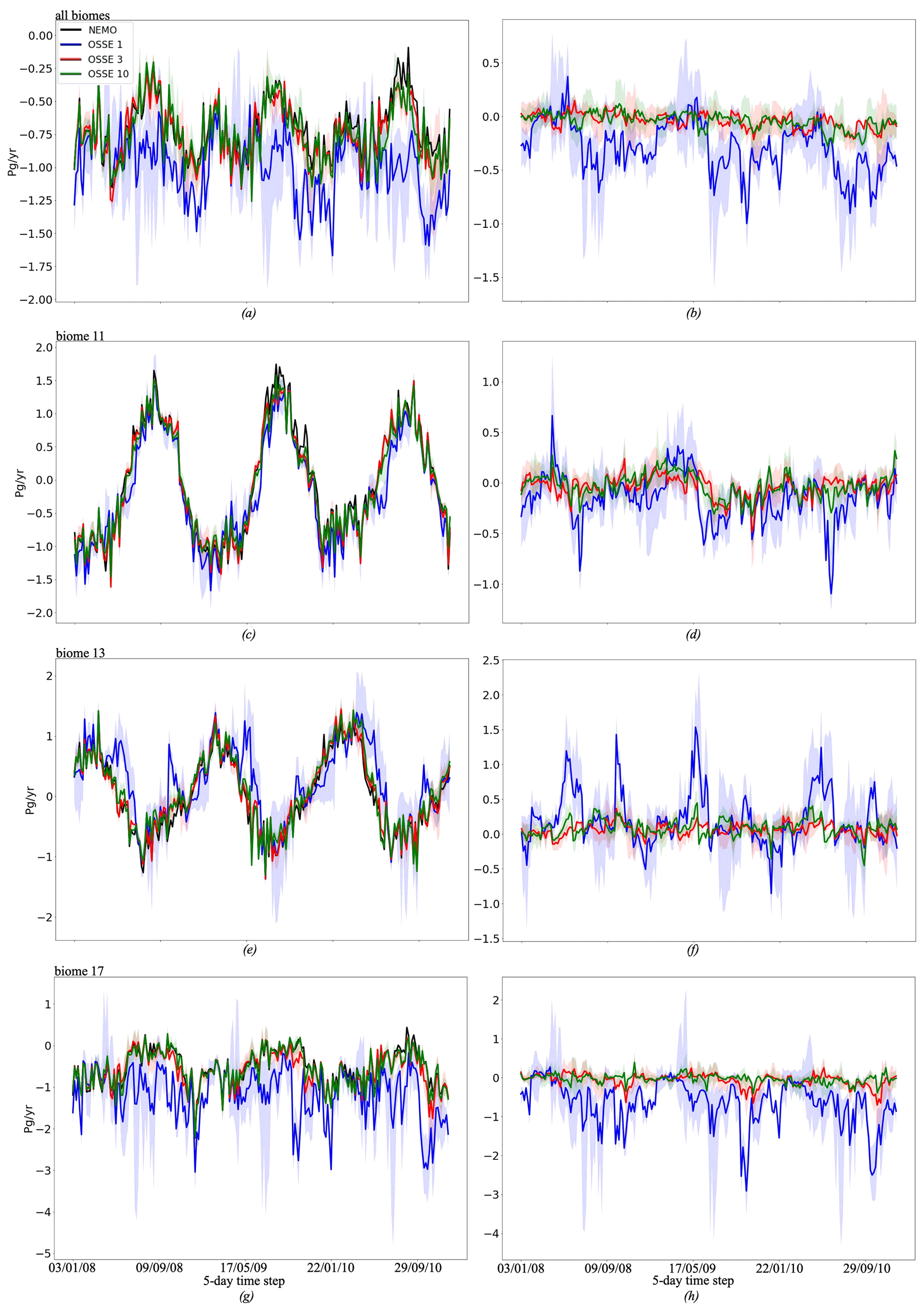
Figure 8 (a, c, e) Mean of fgCO₂ from four FFNN outputs for OSSE 1 (blue) (SOCAT data only), 3 (red) (SOCAT and synthetic Argo data) and 10 (green) (SOCAT data, 25 % of the original synthetic Argo data in the Southern Hemisphere, and data from mooring stations); shading corresponds to the maximum and minimum values from four FFNN fgCO₂ estimates for each OSSE. The black curve shows NEMO/PISCES fgCO₂. (b, d, f) Mean of differences of four FFNN outputs between OSSE 1 (blue), 3 (red), and 10 (green) fgCO₂ and NEMO/PISCES fgCO₂; shading corresponds to the maximum and minimum values of differences from four FFNN fgCO₂ for each OSSE. (a, b) Estimates are available for all biomes presented in Fig. 2, except biome 8: (c, d) biome 11 (subtropical permanently stratified North Atlantic), (e, f) biome 13 (subtropical permanently stratified South Atlantic), and (g, h) biome 17 (Southern Ocean ice).

Table 8 fgCO₂ averaged over the region 80^∘ S–80^∘ N, 70^∘ W–30^∘ E and biomes from Fig. 2 for the NEMO/PISCES model; OSSEs 1, 3, 4, and 10; and the corresponding averaged differences between each OSSEs and NEMO/PISCES (in Pg yr⁻¹).

The relationship between the average number of Argo floats (5 d period) and the error in fgCO₂ estimates (Tables 8, S5) is shown in Fig. 9 for all biomes (a), biome 11 (b), biome 13 (c) and biome 17 (d). Figure 9a illustrates how the increase of the number of floats usually yields a reduction in the error of fgCO₂ estimates. Considering the whole region, OSSE 10 provides the best results with less Argo floats (−0.04 PgC yr⁻¹ and 48 Argo floats). At the biome scale, the addition of floats does not, however, systematically reduce the error. This holds for biome 11 (Fig. 9b), which is well covered by observations, but also for biome 13 with a much sparser data coverage (Fig. 9d). For biome 11, OSSE 10 has the best trade-off between error reduction and number of floats. The largest error (0.22 PgC yr⁻¹) is obtained for OSSE 2 (only Argo data). It suggests that the period chosen for this study is too short to adequately capture the seasonal variability. This hypothesis is supported by the fact that while OSSE 3 and OSSE 2 share the same number of Argo data, OSSE 3 is further constrained by SOCAT data that cover the period 2001–2010. These additional data from SOCAT introduce the information needed for the reconstruction of the seasonal cycle. For biome 13 (Fig. 9c), the combination of SOCAT data and Argo float data improves estimates of fgCO₂. The errors in OSSE 10 are comparable to OSSE 3 (benchmark), 0.08 PgC yr⁻¹ (OSSE 10) and 0.06 PgC yr⁻¹ (OSSE 3). The error is even lower for OSSE 11 (0.04 PgC yr⁻¹), the experiment with the smallest number of Argo floats (19), than for OSSE 3. Unfortunately, results provided by OSSE 11 are less good over the remainder of the biomes. The tendency for a decrease of fgCO₂ error with an increase of the number of Argo floats is confirmed for biome 17 (Fig. 9d). The additional data from mooring stations (OSSE 9, 10 and 11) improve OSSEs with smaller numbers of floats in particular. An error of −0.03 PgC yr⁻¹ is computed for OSSE 10 (49 floats) over biome 17. The results for other biomes can be found in the Supplement (Fig. S18).

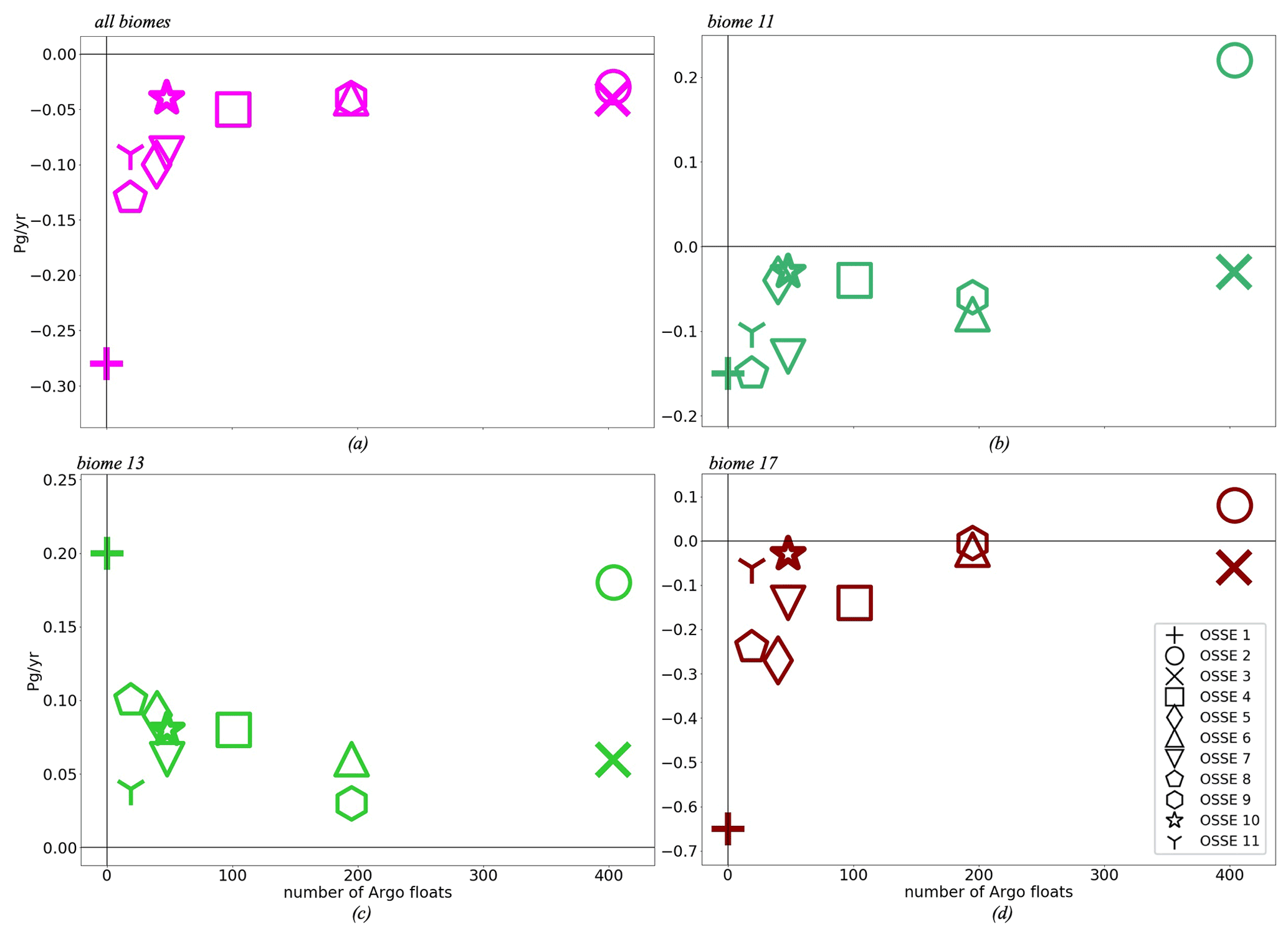
Figure 9 Averaged number of Argo profiles per 5 d time step over 2008–2010 versus averaged differences between each OSSE fgCO₂ and NEMO fgCO₂ (in Pg yr⁻¹), the colour code corresponds to Fig. 2, the purple colour represents the total of the eight biomes: (a) all biomes, (b) biome 11 (subtropical permanently stratified North Atlantic), (c) biome 13 (subtropical permanently stratified South Atlantic), and (d) biome 17 (Southern Ocean ice). OSSE 1 uses SOCAT data only; OSSE 2 uses synthetic Argo data only; OSSE 3 uses SOCAT and synthetic Argo data; OSSE 4 uses SOCAT data and 25 % of the original synthetic Argo data; OSSE 5 uses SOCAT data and 10 % of the original synthetic Argo data; OSSE 6 uses SOCAT data and synthetic Argo data in the Southern Hemisphere; OSSE 7 uses SOCAT data and 25 % of the original synthetic Argo data in the Southern Hemisphere; OSSE 8 uses SOCAT data and 10 % of the original synthetic Argo data in the Southern Hemisphere; OSSE 9 uses SOCAT data, synthetic Argo data in the Southern Hemisphere, and data from mooring stations; OSSE 10 uses SOCAT data, 25 % of the original synthetic Argo data in the Southern Hemisphere, and data from mooring stations; OSSE 11 uses SOCAT data, 10 % of the original synthetic Argo data in the Southern Hemisphere, and data from mooring stations. OSSEs 1, 3 and 10 are in bold as they represent the main OSSEs of our comparisons.

4 Summary and conclusion

The aim of this work was to identify an optimal observational network of pCO₂ over the Atlantic Ocean. The analysis was based on results obtained with a feed-forward neural network model trained on the SOCAT database. The SOCAT database has sparse coverage in the Southern Hemisphere. The approach consisted of adding the position of mooring data and Argo trajectories in the Atlantic Ocean to find an optimal distribution and combination of data to reconstruct pCO₂ with a good accuracy. The advantage of the SOCAT database is the long time period covered by its records, which allows us to reconstruct the interannual variability with a good accuracy. However, its data coverage is biased towards the North Atlantic, which leads to larger reconstruction errors over the South Atlantic by the neural network. As a long-term perspective, the inclusion of data from Argo floats will contribute to a more homogenous data distribution and provide better spatial coverage. The Argo floats and moorings used here do not currently provide pCO₂ measurements, and hence only their positions were used to build OSSEs. A series of experiments were performed using outputs from the NEMO/PISCES model. The model simulations were sub-sampled at co-localised sites of observing platforms for all predictors (SSS, SST, SSH, CHL, MLD, pCO_2,atm) used in the FFNN and the target (pCO₂) to create pseudo-observations with a 5 d time step. These experiments should be useful for the planning of future deployments of BGC-Argo floats (Biogeochemical-Argo Planning Group, 2016) and moorings equipped with the sensors to measure pCO₂ or CO₂ fugacity. In this study we focused on the reconstruction of short-term interannual variability (3 years: 2008–2010) of pCO₂. The results can be different for long-term variability, which will strongly depend on the data availability and data distribution over a longer period (Gloege et al., 2021).

The results suggest that the addition of data from Argo floats could significantly improve the accuracy of FFNN-based ocean pCO₂ reconstructions over the Atlantic Ocean and the Atlantic sector of the Southern Ocean compared to the case when only SOCAT data are used (OSSE 1). However, even with an improved coverage over the open ocean, additional observations are required in coastal regions and shelf seas that are not accessible to floats, as well as in regions with a strong seasonal variability of pCO₂ and all predictors. This is exemplified by OSSE 2, the experiment based on all Argo data, which yields high RMSDs in biome 9, the subpolar seasonally stratified North Atlantic (Figs. 3, 4b, Table 4). The RMSD of 17.1 µatm reflects the poor coverage of this region by Argo floats (Fig. 1b), in particular the Greenland Sea and the North Sea, with a large part of the latter not suitable for the deployment of floats. The combination of SOCAT data and Argo floats (OSSE 3) improves the reconstruction with a RMSD reduced to 9.59 µatm (Fig. 4b, Table 4).

The reduction of the percentage of Argo data used in our experiments slightly decreases the accuracy (Figs. 3 and 4, Tables 3 and 4). A lower percentage of Argo data corresponds, however, to a more realistic distribution of instruments and to the target of the global BGC-Argo network. The results are still comparable to OSSE 3. The best compromise between the statistics yielded by the comparison between reconstructed pCO₂ and NEMO/PISCES outputs, as well as the feasibility of a future observation network, is found for OSSE 10. In this experiment SOCAT data are combined with simulated mooring data and 25 % of the initial distribution of Argo floats placed only in the Southern Hemisphere (around 49 floats with a 5 d sampling period). The use of only SOCAT data results in a correlation coefficient of 0.67 compared to NEMO/PISCES output and a standard deviation of 26.08 µatm (25.34 µatm for NEMO/PISCES) over the region of study. The successful OSSE 10 has a correlation coefficient of 0.85 and a standard deviation of 24.89 µatm. These results are close to the unrealistic benchmark case with total Argo float distribution over 2008–2010: 0.87 and 23.79 µatm. The total pCO₂ over the whole region is also close to NEMO/PISCES, ∼ 370 and ∼ 371 µatm, respectively. The sea–air flux fgCO₂ is −0.83 Pg yr⁻¹ (OSSE 10) and −0.76 Pg yr⁻¹ (NEMO). The bias in sea–air CO₂ fluxes compared to NEMO/PISCES is reduced by 74 % in OSSE 10 compared to OSSE 1 (fgCO₂ is −1.03 Pg yr⁻¹).

The OSSE 10 network could be further improved by instrumenting Baffin Bay, the Labrador Sea, the Norwegian Sea, and regions along the coast of Africa (10^∘ N to 20^∘ S), all regions with pronounced biases in all OSSEs, with moorings or gliders as well as sail-drones and sail buoys along the shelf break and on the continental shelf.

The inclusion of errors from in situ measurements is one of the next steps of this work. The real measurements contain instrumental and representation errors. The inclusion of errors in pseudo-observations will help to estimate the impact of observations on the reliability of OSSEs presented in this work. It will include the errors for predictor values (SSS, SST, SSH, CHL, MLD, pCO_2,atm) that are measured directly or derived from remote sensing (e.g. SST, chlorophyll, SSH), as well as the errors related to the computation of pCO₂ from pH and alkalinity. The new FFNN runs could provide important information on the effect of biases from observational datasets and identify predictors or targets that have large errors and thus must be corrected. The consistent introduction of error estimates for each predictor will provide this information.