Glider-based observations of CO₂ in the Labrador Sea

Ocean gliders can provide high-spatial- and temporal-resolution data and target specific ocean regions at a low cost compared to ship-based measurements. An important gap, however, given the need for carbon measurements, is the lack of capable sensors for glider-based CO₂ measurements. We need to develop robust methods to evaluate novel CO₂ sensors for gliders. Here we present results from testing the performance of a novel CO₂ optode sensor (Atamanchuk et al., 2014), deployed on a Slocum glider, in the Labrador Sea and on the Newfoundland Shelf. This paper (1) investigates the performance of the CO₂ optode on two glider deployments, (2) demonstrates the utility of using the autonomous SeaCycler profiler mooring (Send et al., 2013; Atamanchuk et al., 2020) to improve in situ sensor data, and (3) presents data from moored and mobile platforms to resolve fine scales of temporal and spatial variability of O₂ and pCO₂ in the Labrador Sea. The Aanderaa CO₂ optode is an early prototype sensor that has not undergone rigorous testing on a glider but is compact and uses little power. Our analysis shows that the sensor suffers from instability and slow response times (τ₉₅>100 s), affected by different behavior when profiling through small (<3 ^∘C) vs. large (>10 ^∘C) changes in temperature over similar time intervals. We compare the glider and SeaCycler O₂ and CO₂ observations and estimate the glider data uncertainty as ± 6.14 and ± 44.01 µatm, respectively. From the Labrador Sea mission, we point to short timescales (<7 d) and distance (<15 km) scales as important drivers of change in this region.

1 Introduction

The ocean plays a crucial role in absorbing the effects of changes to the Earth's atmospheric composition due to anthropogenic activities. Roughly one-third of all human-made CO₂ (C_ant) released into the atmosphere since the beginning of the industrial revolution has been taken up by the ocean, a total of 155 ± 31 GtC as of 2010 (Khatiwala et al., 2013). For the decade 2009–2018 alone, the global ocean carbon sink absorbed 2.5 ± 0.6 GtC yr⁻¹ against fossil fuel emissions of 9.5 ± 0.5 GtC yr⁻¹ (Friedlingstein et al., 2019). Ocean carbon sinks are not equally distributed across the globe. Very intense carbon sinks and regions of anthropogenic carbon storage are located in subpolar ocean regions (Volk and Hoffert, 1985; Sabine et al., 2004), such as the Labrador Sea in the North Atlantic (DeGrandpre et al., 2006) and the Southern Ocean's Weddell Sea (van Heuven et al., 2014). Deep mixing in these regions is adding anthropogenic carbon to the deep ocean water mass transports, linking these high-latitude carbon pumps to the global ocean (Broecker, 1991; Fontela et al., 2016). Increased carbon storage in the ocean has, over the past decades, caused pH levels to drop in many places (Doney et al., 2009) at a rate of change that is faster than found in the geological record (Zeebe et al., 2016). Resulting ocean acidification (OA) has already severely impacted marine habitats worldwide, including such important ecosystems as the Great Barrier Reef (Cohen and Holcomb, 2009; Guinotte and Fabry, 2009).

Predicting shifts in future carbon uptake scenarios requires a detailed understanding of the processes driving uptake and distribution of absorbed carbon across all oceanic scales. We need to advance the global ocean carbon measurement system because existing observations are limited in coverage and quality (Borges et al., 2010; Okazaki et al., 2017). There have been recent advances in autonomous sampling strategies to expand, improve, and build on existing global biogeochemical observing networks (Johnson et al., 2009). The existing Argo float program is expanding, including biogeochemical (BGC-Argo) sensors measuring oxygen, nitrate, chlorophyll, turbidity, irradiance, and pH. BGC-Argo aims to observe seasonal- to decadal-scale variability, although currently only about 8 % of Argo floats are equipped with biogeochemical sensors (Johnson et al., 2017; Li et al., 2019). Improvements in resolution and frequency of surface CO₂ measurements have also come from developing stable ship-based in situ measurement systems installed on container ships and tankers with regular routes across ocean basins. These results made possible the creation of the 1^∘ global resolution (up to 1∕4^∘ coastal zones) Surface Ocean CO₂ Atlas (Bakker et al., 2016). However, these data do not provide at-depth information needed to understand the localized processes that drive and shape the strength of carbon sink regions such as the Labrador Sea. Advances in glider technology and sensors (Rudnick, 2016; Testor et al., 2019) can help address those gaps.

Advancing glider-based measurements of CO₂ requires addressing key issues such as stability, responsiveness, compactness, and power consumption (Clarke et al., 2017a, b; Fritzsche et al., 2018). Another important factor is to ascertain the uncertainty of sensor-based observations (Newton et al., 2015). So far, most carbon glider observations are limited to testing, and concerns remain about data quality. The most mature and commonly used type of in situ CO₂ probe is based on infrared (IR) detection, such as the CONTROS Hydro C™ and Pro Oceanus CO₂-Pro CV™ sensors. Unfortunately, commercial IR-based detection systems are not yet small enough to easily fit existing gliders or float designs. Long equilibration times make profiling applications of sensors extremely challenging, requiring detailed knowledge of response times and data processing (Fiedler et al., 2013; Atamanchuk et al., 2020). These sensors are also very power-hungry compared to other sensors like optodes and conductivity–temperature–depth casts (CTDs), making battery-powered deployments challenging even for moored applications. Another approach to determining in situ CO₂ is through pH measurements using established total alkalinity (A_T) and salinity (S) relationships (Takeshita et al., 2014). Saba et al. (2018) applied a novel ISFET pH sensor (Johnson et al., 2016) developed by MBARI with help from Sea-Bird Scientific on a glider. These tests showed remarkable response time characteristics and stability over periods of several weeks or longer.

Another candidate for glider carbon observations is the Aanderaa CO₂ optode sensor (Atamanchuk et al., 2014). It is nearly identical in size and power consumption to the commonly used oxygen optode by the same company but lacks prior glider testing. The optode detects the luminescent-quenching response from a CO₂-sensitive membrane. In general, there are multiple challenges to using photochemical sensors on profiling applications (Bittig et al., 2014): (1) placement of the sensor on the glider dictates boundary layer thickness and response time; (2) response time is nonlinearly temperature-dependent, and steep temperature gradients induce additive error; and (3) the sensor is highly dependent on prior foil calibration and can suffer from drift. In particular, the foil design has multiple temperature-dependent rate-limiting processes inside the foil to sense the ambient change in pH, which relates to changes in pCO₂ (Sergey Borisov, personal communications, 2019). On the upside, the CO₂ optode is an attractive candidate for gliders due to its small size, ease of integration, and low power consumption, all similar to the Aanderaa oxygen optode. Because of the need for increased spatial and temporal resolution of CO₂ observations and the advantages gliders offer compared to other methods, assessing the CO₂ optode on a glider is an important step in furthering community knowledge of the current state of mobile CO₂ system technology.

In 2016, as part of the Ventilation, Interactions and Transports Across the Labrador Sea (VITALS) project, we devised an observing strategy to carry out novel in situ observations to (1) reach the deep convection region with a glider to carry out sampling with the novel foil-based pCO₂ sensor from Aanderaa with minimal ship resources for launch and recovery. (2) We use measurements provided by an autonomous moored profiler – the SeaCycler (Send et al., 2013), carrying the larger-payload CO₂-Pro CV instrument for glider in situ calibration points. This mission attempted to use a moored sensing platform as an in situ reference point for experimental sensors deployed on a glider to advance data quality and coherence of novel biogeochemical measurements. As technology plays a catch-up game, such mission concepts will be important in the next steps towards targeted oceanic carbon measurements. We re-deployed the glider in September 2018 on the Newfoundland Shelf in Trinity Bay to further test the concepts from VITALS, flying the glider near a small fishing boat from which reference casts were taken using a similar CO₂-Pro CV instrument. We utilize these two real ocean deployments to improve sensor characterization and the quality of the collected data. In this paper, we present the data, our analysis, and a discussion around three central questions.

• How suitable is the CO₂ optode for glider-based applications?

• How can multiple autonomous platforms be used to improve sensor data?

• How can combined data from moored and mobile platforms resolve scales of temporal and spatial variability?

Addressing these questions should improve and shape our plans for carbon-observing systems utilizing gliders and other platforms, especially as new sensors are being developed.

2 Data and methods

2.1 Labrador Sea deployment

In fall 2016, a moored vertical profiler, the SeaCycler (Send et al., 2013; Atamanchuk et al., 2020), and a G2 Slocum glider were deployed into the central Labrador Sea near the longtime German deep convection mooring K1 (Fig. 1). The K1 mooring, located about 25 km west of former OWS Bravo (Avsic et al., 2006), has been deployed biennially since 1994 to monitor activity in the central deep convection patch in the Labrador Sea (Lavender et al., 2002; Koelling et al., 2017). The objective of VITALS was to characterize the spatial and temporal structure of oxygen and CO₂ in the deep convection zone. Other activity in conjunction with VITALS included a hydrographic section AR7W maintained by the Bedford Institute of Oceanography (BIO) and Argo floats released with several profiles captured near the SeaCycler site and the glider deployment area. Many observing efforts came together, utilizing multiple complementary efforts across different scientific programs and relying on traditional and novel observational approaches.

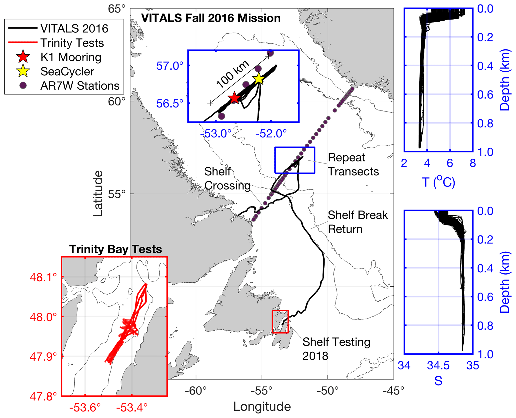
Figure 1 Map of data collection sites: the main map (center) shows the Ventilation, Interaction and Transport Across the Labrador Sea (VITALS) glider track, with the blue inset focusing on the repeat transects along the AR7W line. Contours are the 1500 and 3000 m isobaths. Highlighted in blue are also the corresponding T–S profiles collected by the glider in that time period. Salinity is given in practical salinity units. The red inset map in the lower left shows the glider track from the 2018 glider CO₂ optode tests conducted in Trinity Bay, NL.

The SeaCycler was deployed near 52.22^∘ W and 56.82^∘ N, 30 km away from the German deep convection mooring K1 (52.66^∘ W and 56.56^∘ N), to improve the vertical and temporal characterization of O₂ and CO₂ cycling in this region. The SeaCycler operation and deployment techniques are described in Send et al. (2013). It has an underwater winch assembly parked at of 160 m depth with an instrument float that can profile the top 150 m. Tethered communication allows for two-way telemetry over the Iridium satellite. Below the winch assembly, a single-point mooring line with instruments continues to the ocean depth of approximately 3500 m. For this deployment, the instrument float carried a CTD, velocity, and various gas sensors, including oxygen sensors (Sea-Bird 43, Sea-Bird 63, Aanderaa 4330) and the CO₂ optode prototype sensor 4797 as well as the membrane-equilibrator-based infrared (IR) CO₂ gas analyzer CO₂-Pro CV based on non-dispersive infrared refraction (NDIR) technology made by Pro Oceanus Ltd, Canada (https://www.pro-oceanus.com, last access: 17 December 2020). Previous tests with a similar sensor design showed excellent stability in multi-month vessel-underway missions (Jiang et al., 2014). The instrument float collected data over the top 150 m of ocean depth with an average resolution of 0.3 m from June 2016 to May 2017, while the Pro CV was sampling for 20 min at selected stop depths (10, 30, 60, 120 m) to allow equilibration with ambient seawater pCO₂. These stops resembled bottle stops done from ships with the water rosette to validate new sensors. The K1 mooring was also equipped with oxygen sensors to allow for later cross-mooring comparisons. The SeaCycler data were corrected for sensor drift using pre- and post-deployment calibration of the sensors (Atamanchuk et al., 2020). The oxygen data were also corrected for a response time delay using the response time values from Bittig et al. (2014) and the algorithm described in Miloshevich et al. (2004). Overall, the accuracy of the oxygen data was 2.89 ± 4.17 µM based on residuals between the upcast and discrete downcast data. The Pro CV had a zero-referencing routine that corrected the drift of the zero point of the sensor (Atamanchuk et al., 2020). Fully equilibrated pCO₂ data were obtained by averaging the last 30 s of the measurements at each stop depth. Accuracy of pCO₂ data was determined from the accuracy of the instrument, i.e., 0.5 % over the full range (0–1000 µatm) with an initial manufacturer-quoted accuracy of ±2 µatm.

The glider (Unit 473) was deployed from the Labrador Shelf to reach the K1–SeaCycler site and complete 30 to 100 km long transects between the two moorings, collecting high-resolution spatial data. The glider was launched near Cartwright, Labrador, from a small fishing boat and reached the deep convection zone near K1 and SeaCycler early in October, sampling there until 22 November. In total, the glider completed 18 full transects, collecting valuable hydrographic and gas data. The modified glider with an extended battery bay carried Sea-Bird glider payload CTD, the Aanderaa Data Instrument (AADI) CO₂ optode prototype sensor (model 4797) described in Atamanchuk et al. (2014), and the well-established Aanderaa oxygen optode (Tengberg et al., 2006) model 4831, SN 333. Glider CTD manufacturer calibration showed an initial accuracy better than ± 0.0005 S m⁻¹, ± 0.005 ^∘C, and 0.1 % of the total pressure range. The initial accuracy of the calibrated O₂ optode from the manufacturer was better than ± 4 µM. Accuracy of the CO₂ optode pre-deployment was unknown, but the accuracy range in Atamanchuk et al. (2014) is ± 2–75 µatm. The CO₂ optode (SN57) was equipped with a standard foil to enhance deployment stability. These optode sensors were mounted in the aft cone of the vehicle. Also, a thruster was installed to speed up the shelf's crossing and enable staircase profile sampling. The glider sampled in the central Labrador Sea for 2 months, limiting CO₂ optode profiles to the top 200 m to save energy. In December, the glider began its journey back to Newfoundland, following the 1500 m isobath inside the Labrador Current and reaching Trinity Bay (see map) on 31 December 2016. The glider was flown along the shelf break to take advantage of the southward-flowing Labrador Current. Before deployment on the glider, the CO₂ optode underwent testing at the CERC.OCEAN laboratory at Dalhousie University to determine the calibration model fit for the optode sensor foil.

2.2 Trinity Bay tests

After completing the VITALS mission, to further test all the characteristics of the new CO₂ optode under glider profiling tests, we conducted another study in Trinity Bay, Newfoundland. Trinity Bay is a deep inlet (up to 600 m) and can be reached easily from various coastal communities from a fishing boat. It is fed primarily by the cold Labrador Current waters and river runoff from the western side, making its surface waters fresh and deeper portions cold, highly oxygenated, and nutrient-rich. The pooling of water in the deeper portion and surface fresh water supports a stable density stratification (Schillinger et al., 2000; Tittensor et al., 2002). Especially interesting for our optode tests are the large vertical temperature changes of over 14 ^∘C between the surface and 75 m of depth. Trinity Bay has a cold water lens of −1 ^∘C between 70 and 200 m of depth (Fig. 2d) and temperatures below 1 ^∘C from 200 m to the bottom. In Trinity Bay, profiling through this lens leads to absolute temperature gradients of 10 ^∘C or more in 200 s or less.

In Trinity Bay, we repeated the VITALS data comparison experiment on a smaller scale without using a SeaCycler. To collect in situ reference samples, we used a winch-operated Sea-Bird 19+ V2 CTD mounted on a frame, together with an O₂ optode (model 4831, SN 333) and a CO₂-Pro CV. We repeated staircase missions as in VITALS and did extensive calibration of the sensor before and after the deployment. The glider was deployed from 4–16 September 2018. The setups for the external winch-operated CTD and glider are summarized in Fig. 2a and b.

Table 1 Sensor offsets from DFO tank tests on 27 August 2018.

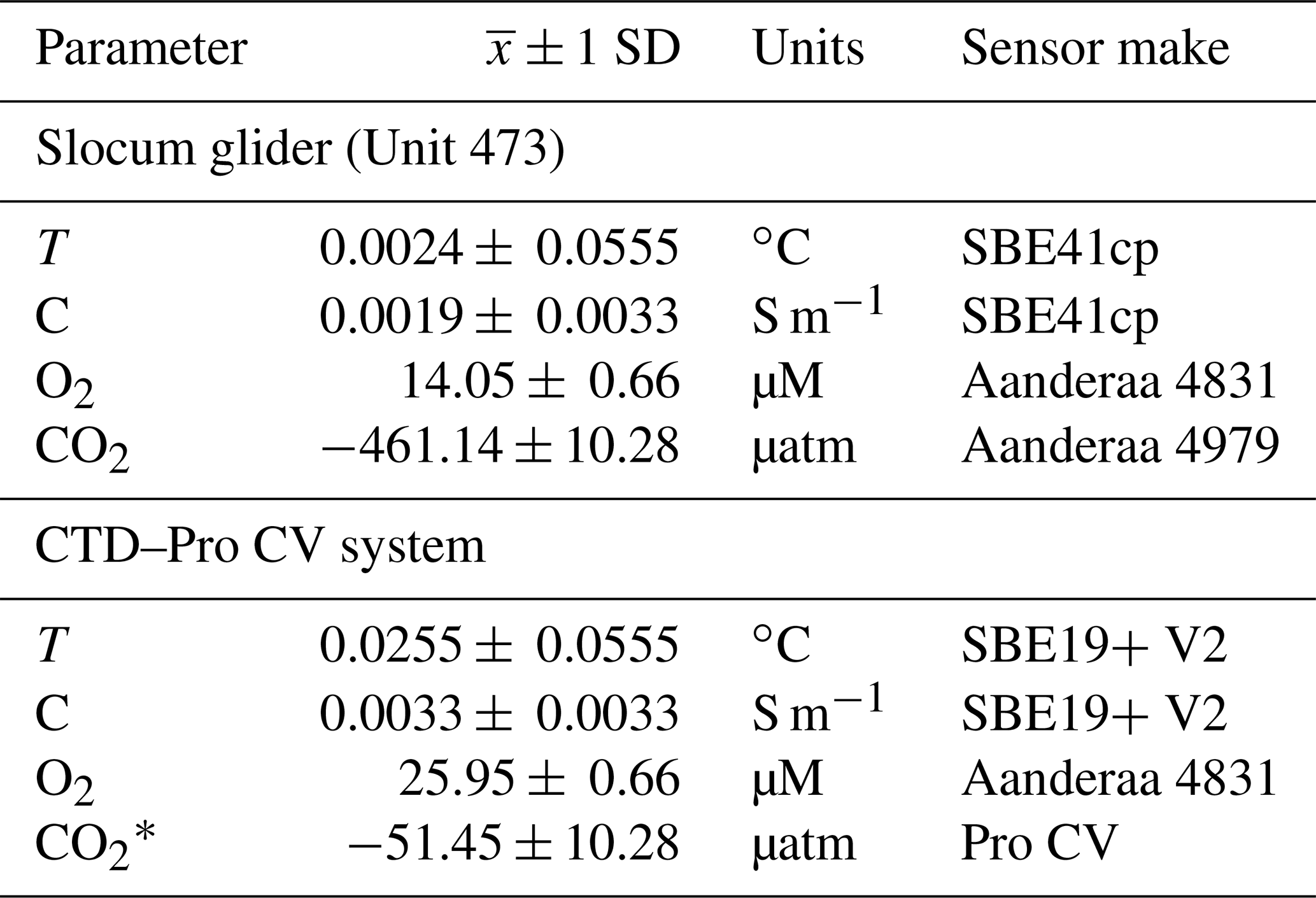
^* Note: CO₂-Pro CV was located close to the tank's inlet, which could be the cause of the large offset.

Pre-mission laboratory testing of the sensor and the glider allowed for instrument data quality control in this mission. The glider CO₂ and O₂ optode sensors were calibrated at the CERC.OCEAN laboratory at Dalhousie University using a double-walled test tank, with simultaneous O₂ and CO₂ supply for rapid step changes in these variables. The optode sensor response in the range of −1.8 to 20 ^∘C, O₂ concentrations ranging from 0 % to 120 % saturation, and CO₂ concentrations from 100 to 3000 µatm were used to compute the CO₂ optode foil coefficients. Tests were initially done in fresh water and repeated for 35 ppt NaCl solution. Further, tests of glider sensors together with the CTD–Pro CV setup were done inside a saltwater tank at the Department of Fisheries and Oceans (DFO) in St. John's, Canada. The tank allows simultaneously submerging the glider, CTD–Pro CV setup, and a CTD rosette (SBE9) with Niskin bottles to obtain reference O₂, A_T, dissolved inorganic carbon (DIC), T, and S data. A summary of the water sample analysis and uncertainty is given in Appendix A. Based on the tank tests, we estimate initial sensor offsets for the glider and the CTD–Pro CV. Table 1 summarizes results from the DFO tank tests. Reported uncertainties are the combined uncertainty of the measured offsets ($\stackrel{\mathrm{‾}}{x}$) from tank tests, including the uncertainty from the lab-based results (± 1 SD) and the manufacturer's sensor accuracy. SD in the text refers to the sample standard deviation. A picture of tank testing in progress is shown in Fig. 2c. The location of the CO₂-Pro CV (bottom left) during the tank tests is close to an inlet, which may have caused a noticeable difference in CO₂ values. Before the deployment, we find an initial offset of −461.14 µatm for the glider CO₂ optode. However, the sensor had not yet undergone conditioning. Other sensors (CTD, O₂ optode) show good agreement among each other, with the collected water samples giving a good initial reference for the sensors.

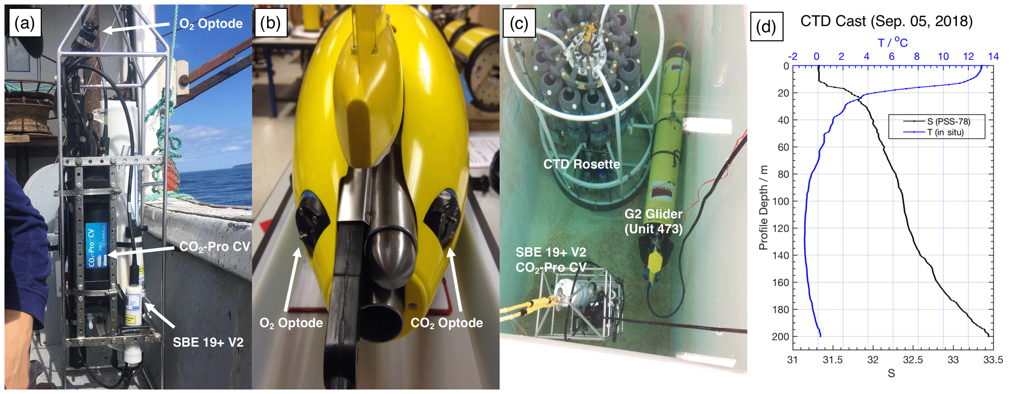
Figure 2 (a) Trinity Bay test reference CTD, (b) glider setup, (c) equipment tank testing in progress, and (d) average T–S structure observed from shipboard casts on 5 September 2018.

2.3 Glider data processing

We processed glider science data, correcting the CTD data for temperature-induced sensor lag and applying sequential comparison between glider profiles Garau et al. (2011). Salinity is calculated from temperature and conductivity using the practical salinity scale. To correct the phase response lag in the glider oxygen data, we applied the model published in Bittig et al. (2014) using raw sensor phase-angle output. Instead of using the built-in optode thermistor, we used the lag-corrected CTD temperature readings interpolated to the optode measurements as in Gourcuff (2014). From the corrected phase readings, we computed the molar oxygen concentrations (µM or µmol L⁻¹) using Uchida et al. (2008), with fit constants from a prior optode tank calibration. Trinity Bay tank test and ship-based CTD profiles provided further calibration points at the start and end of the deployment.

For the CO₂ optode, there was some literature available for temperature-dependent response time corrections (Bittig et al., 2014). However, each sensor has response time characteristics that must be determined before any field deployments. Due to the dual lifetime referencing (DLR) technique in the foil and available field results, the sensor response is larger than the O₂ optode, which uses more straightforward foil chemistry. To correct for the long response time behavior, we used a sequential time-lag correction (Eq. 1) approach (Miloshevich et al., 2004), recently applied for an equilibrator-type NDIR gas instrument (Fiedler et al., 2013). In Fiedler et al. (2013), the NDIR instrument was mounted on a profiling float, and response times are calculated to be on the order of 100–300 s between surface and depth measurements.

$$\begin{array}{}\text{(1)}& c_{i+\mathrm{1}}^{\mathrm{cor}}={\displaystyle \frac{c_{i+\mathrm{1}}^{\mathrm{in}\mathrm{situ}}-\left[c_i^{\mathrm{in}\mathrm{situ}}\exp \left(-\mathrm{\Delta }t/\mathit{\tau }\right)\right]}{\mathrm{1}-\exp \left(-\mathrm{\Delta }t/\mathit{\tau }\right)}}\end{array}$$

Here c^in situ is the raw and c^cor is the corrected sensor output at each time step i. The time constant τ can be computed by fitting an exponential model to the sensor response x(t) (Eq. 2) using the fitting constants a and b at each time interval dt.

$$\begin{array}{}\text{(2)}& x\left(t\right)=(a-b)\exp \left(-\mathrm{d}t/\mathit{\tau }\right)+b\end{array}$$

Atamanchuk et al. (2014) provided a few values for the response time. Temperatures were much warmer than found in the Labrador Sea and Trinity Bay and did not provide response characterization for varying temperature gradients. Fiedler et al. (2013) used an exponential model (Eq. 2) to compare their NDIR sensor's response to zero measurements (ZMs). During ZMs, the sensor strips the gas stream of CO₂, and the resulting reading should be zero. The time response of the sensor and resulting reading after ZM were used to gauge the sensor's response to smaller gas gradients and drift of the gas detector itself. Because the optode sensor does not have the internal capability for independent referencing of the foil chemistry, we fitted the equation to the sensor response while the glider ascended or descended through the thermocline. Repeating this procedure for both glider deployments, we computed a temperature- and response-time-dependent set of values.

The staircase glider profiles in Trinity Bay were performed to help characterize sensor response to a broader set of positive and negative temperature gradients. Staircase profiles in Fig. 3 show the least-squares fit for a single temperature gradient and optode response excursion. To compute the partial pressure of CO₂ (pCO₂) in micro-atmospheres (µatm) from the sensor's corrected phase readings, we applied a calibration fit model from previous tank calibration done at the CERC.OCEAN laboratory at Dalhousie University as was done in previous deployments of this sensor (Atamanchuk et al., 2015; Peeters et al., 2016). A testing regime of temperature and molar xCO₂ concentration step changes as well as sensor phase response readings was used to compute an 8^∘ phase and 3^∘ temperature model fit, which we applied to the sensor. The sensor data and calibration coefficients are available online (von Oppeln-Bronikowski, 2019).

The CO₂ optode sensor exhibits noticeable conditioning behavior (Atamanchuk et al., 2015). After the sensor stabilized, we subtracted an offset (1275 µatm) for the VITALS deployment based on the surface SeaCycler and atmospheric data to correct the optode sensor to ambient conditions. We estimated the timescale of conditioning by fitting an exponential curve to the optode data to find the time constant at which the sensor response plateaued. In the VITALS deployment, conditioning took almost a month into the deployment, while in Trinity Bay tests, the sensor response stabilized after 4 d (offset of 994 µatm). During the last 1.5 d of the Trinity Bay tests, the sensor displayed inconsistent behavior with depth. Data from the final 1.5 d were excluded from further analysis. It is not clear what caused this change in the sensor's response. Perhaps cold temperatures in Trinity Bay ($<-\mathrm{1}$ ^∘C) caused the foil to degrade.

To help with visualization, we bin-averaged the data and mapped the data along isopycnals. For some cross-sectional plots, we also averaged data in depth–space or depth–time sections. To account for the gaps in observations, we preserved gaps larger than 10 km and more prolonged than 4 d. Smaller gaps were linearly interpolated. A 3D boxcar filter was applied to smooth 5 km in the horizontal, 5 m depth, and 3 d in time, keeping with the observing gaps in the data because the glider occupied a section between K1 and SeaCycler every 2 to 3 d, and gaps between profiles were 3 km on average.

To grid the sparse O₂ and pCO₂ glider observations for spatial–temporal data intercomparison with SeaCycler, we deviated from linear interpolation. We used an objective interpolation method using a second-degree polynomial fitting distance-weighting scheme following Goodin et al. (1979). We gridded the sparse data on a 1 km by 1 d grid and then interpolated the data using an exponential weighting function $\exp (R_x^{-\mathrm{2}}+R_y^{-\mathrm{2}})$ to fill in gaps. We determined influence radii of approximately 5 km for O₂ and 20 km for pCO₂ measurements and cutoffs at 10 and 40 km, respectively, based on the number of glider observations in the horizontal and along the time dimension. We set the cutoff radius at twice the spatial scale. Temporal scales are similar between the two datasets, with an influence radius of 3 d and a cutoff of 6 d.

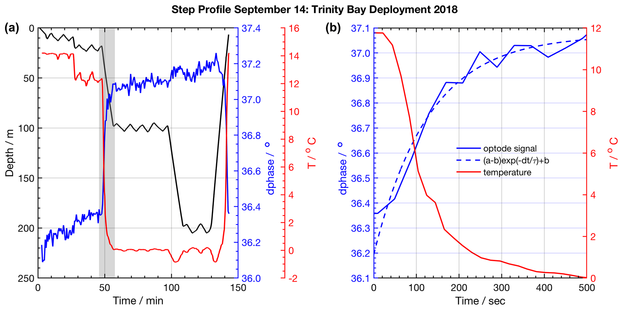
Figure 3 Example of a staircase profile used to quantify response time characteristics. (a) Glider staircase profile (black) overlaid with glider CTD temperature (red) and CO₂ optode signal (blue). The grey shaded area highlights an example episode of sensor response, shown in (b), used to quantify the sensor response time and correct glider profiles. The exponential fit to the CO₂ optode response is shown (dashed blue line).

2.4 Shipboard CTD and Pro CV casts

The Trinity Bay CTD profiles, together with the O₂ optode and data from the Pro CV, were processed by checking for outliers in the profiles. Despite the use of a pump, the Pro CV showed long signal equilibration periods (τ₉₅ between 10 and 15 min). To compute the CO₂ levels for each time the CTD was parked at depth, we took the average of the CO₂-Pro CV values once readings stabilized to within ± 6 ppm or twice the manufacturer's quoted instrument accuracy (0.5 % of the total range 0–600 ppm). We developed a simple script that identified the first time window when the difference in sensor readings reached ΔCO₂≤6 ppm. Pro CV ZMs were subtracted from bottle stops to arrive at a high-quality in situ referenced dataset. We calculated the standard deviation for each set of averaged Pro CV measurements and flagged any data points as outliers when the standard deviation exceeded ± 6 ppm. Those data points were not included in the sensor data comparisons.

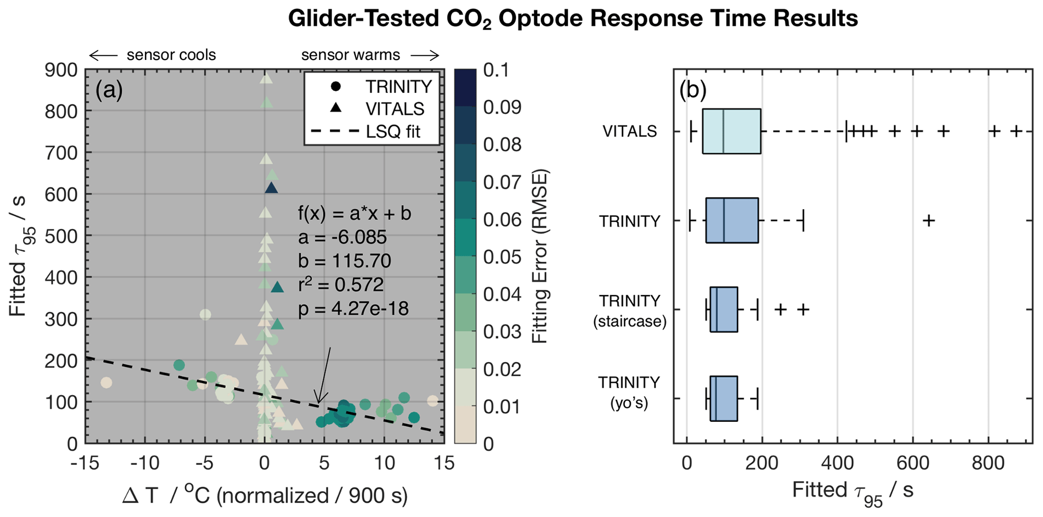
Figure 4 Panel (a) shows the CO₂ optode τ₉₅ values vs. temperature gradients ΔT normalized by dt=900 s and color-coded for the root mean square error (RMSE) of fits to the exponential model $x\left(t\right)=(a-b)\exp (-\mathrm{d}t/\mathit{\tau })+b$. Distinct markers are used to differentiate between the VITALS and the Trinity glider data. The dashed line indicates a linear least-squares (LSQ) fit. Panel (b) shows box plots of the fitted CO₂ optode τ₉₅ values from VITALS and Trinity Bay deployments. The Trinity data are divided into staircase profiles and regular yo's.

3 Results and discussion

3.1 Glider-based CO₂ optode performance

Before this study, the CO₂ optode response had not been studied on a glider, and little information was available about its response time characteristics when profiling. We assess the sensor response time by fitting the raw “dphase” sensor signal (ϕ_DLR) with the earlier described exponential model (Eq. 2) during periods when the glider traversed through temperature gradients. From Eq. (2), we use a response time definition of τ₉₅, which is the time to reach 95 % of the total signal level. The larger a sensor's τ value, the longer it takes the sensor to respond to a change in ambient conditions. We use regular yo and staircase profiles from VITALS and Trinity Bay missions to do a comparative analysis of the sensor response time against observed temperature gradients (ΔT). The VITALS data are regular glider profiles (yo's). Only a few staircase profiles from VITALS were available; they were of low quality and are excluded from this analysis. The Trinity data are mostly regular yo's with nine staircase profiles from 3 d during the deployment (e.g., Fig. 3). For both glider tests, we used data for the period after which the sensor had become conditioned to the environment as described earlier.

Figure 4a shows the result of response time fitting against the temperature gradient (ΔT) normalized by the total time of traversing the gradient (dt) and the sensor response (e.g., ${\mathit{\tau }}_{\mathrm{95},\mathrm{normalized}}={\mathit{\tau }}_{\mathrm{95}}/\mathrm{\Delta }T\times \mathrm{900}$ s). We define ΔT as the total temperature change observed in the interval. We multiply normalized values by 900 s or 15 min to arrive at a set of equally referenced temperature gradient and response time values, all corresponding to the same time interval. We chose this interval based on the response time (τ₉₅≈15 min) of the reference sensing system used in the deployments, the Pro CV. We excluded data from time segments shorter than 60 s, longer than 60 min, and τ₉₅>900 s. The VITALS data show increased τ₉₅ value scatter for small temperature gradients, with no noticeable trend in temperature. The Trinity Bay tests reveal a slight bias in increasing response times with negative temperature gradients. This would indicate that the sensor performs better during upcasts than downcasts. We show linear least-squares fits through the Trinity Bay data points, ignoring the large scatter in VITALS data in the fitting result. Figure 4b summarizes the response time between the deployments. The Trinity data are further divided into the staircase profiles and regular yo's. Contrary to our expectation, the staircase profiles did not noticeably reduce the spread of response times compared to regular yo's. A possible explanation is that the staircase profiles are close to when the sensor was still conditioning and when the sensor began to show a strange response near the end of the mission. Only one full staircase mission was done in the middle of the deployment (10 September 2018). A summary of the analysis of the two datasets is given in Table 2.

Table 2 Response time values from glider-based CO₂ optode tests.

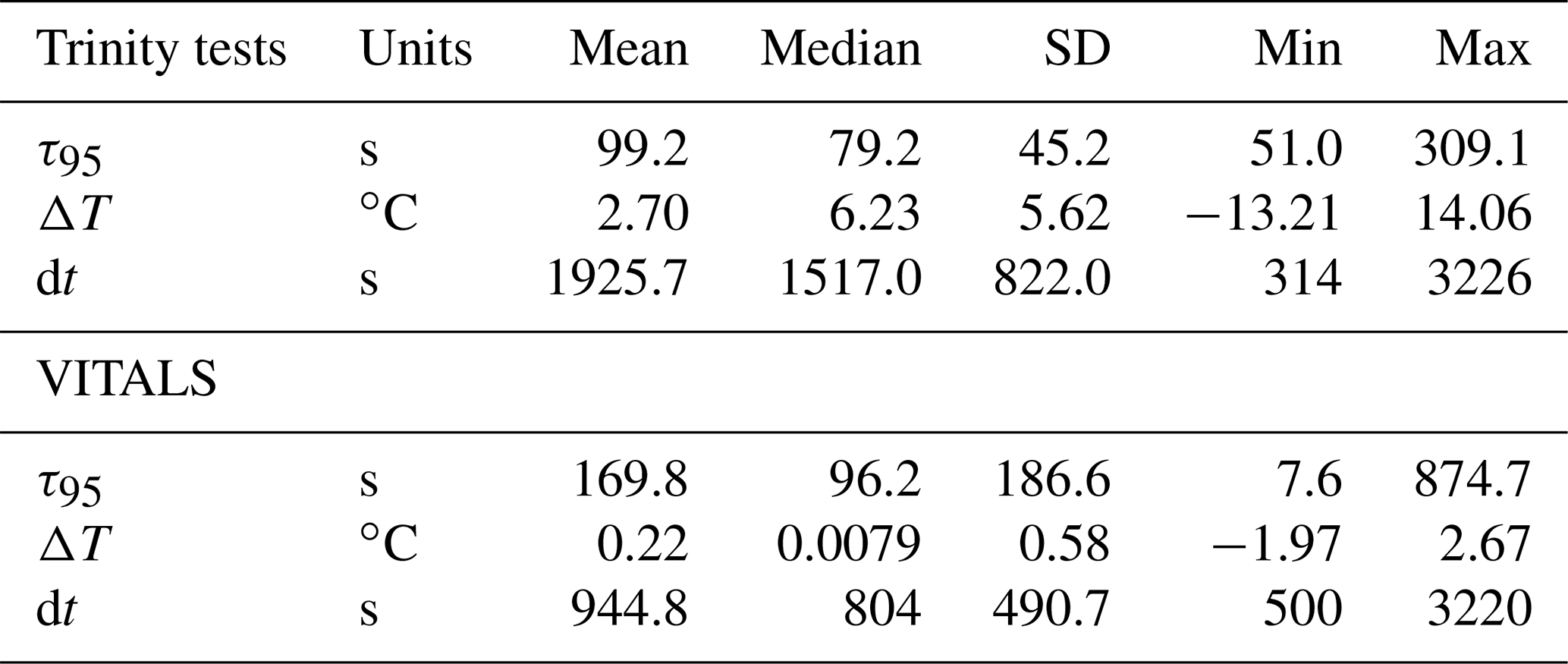
Based on our analysis, we find a median sensor response time (τ₉₅ values) of 79.2 s for the Trinity tests and 96.2 s for the VITALS data, with a mean and standard deviation of 99.2 ± 45.2 and 169.8 ± 186.6 s, respectively. The range of observed response times in Trinity was 51.0–309.1 s. In the VITALS data, the τ₉₅ range is much larger (7.6–874.7). At the same time, ΔT gradients are smaller at 0.22 ± 0.0079 ($\stackrel{\mathrm{‾}}{x}$ ± SD) compared to Trinity Bay with 2.70 ± 5.62. In the Labrador Sea, stratification is greatly reduced compared to Trinity Bay, and temperature gradients are typically small (<3 ^∘C). One would expect shorter response times for smaller temperature gradients. In Trinity Bay, the sensor encountered water temperatures colder than 0 ^∘C. From this analysis alone, it is not clear if there is a permanent effect on the sensor from these cold temperatures. However, Fig. 4a does show an increase in response time values when a sensor cools. Not enough data were collected in Trinity Bay to see if this temperature gradient bias changes or persists over time. Interestingly, the sensor signal (ϕ_DLR) range in the VITALS deployment was different than in Trinity Bay, despite the broader temperature range encountered and similar range in pCO₂. It is possible that some bleaching of the foil had occurred from sunlight despite our best efforts to keep the glider surface time to a minimum.

More work will be necessary to develop a proper response time model. We also did not consider applying a boundary layer and fluid flow model for the optode, such as considered by Bittig et al. (2014) for oxygen optodes. Improvements to the sensor response time and more tests are required to evaluate the influence of the flow field on the sensor performance.

3.2 Comparison: glider and SeaCycler O₂ and CO₂ observations

A novel aspect of the VITALS deployment was the simultaneous measurement of O₂ and CO₂ from a glider and the SeaCycler profiler, allowing both space- and time-varying observations. Given the challenges with validating the glider-based CO₂ optode observations, we used the SeaCycler as an in situ reference for the glider data. For context, the glider and SeaCycler had about 2 months of overlapping observations. Figures 5 and 6 show the time series data from the SeaCycler and monthly averaged panels from the glider transects. The SeaCycler record is divided into distinct periods coinciding with large changes in the at-depth concentration of O₂ and CO₂. The glider measured both the spatial and temporal evolution of the processes captured by the SeaCycler. Figure 6 shows monthly averaged panels (approximately 10 glider passes distance-averaged per month) of the glider data. The much lower spatial density of CO₂ glider profiles (at 15–20 km intervals) compared to O₂ (at least 5 km) means that the CO₂ data resolve only spatial features with scales larger than 20 km compared to a 5 km resolution for O₂. Overall, this region is relatively uniform, with low spatial gradients. Consistent with the SeaCycler observations, we see a flip between concentrations in O₂ and CO₂ between October and November. We also note the different thickness of mixed layer regions across the spatial domain in November.

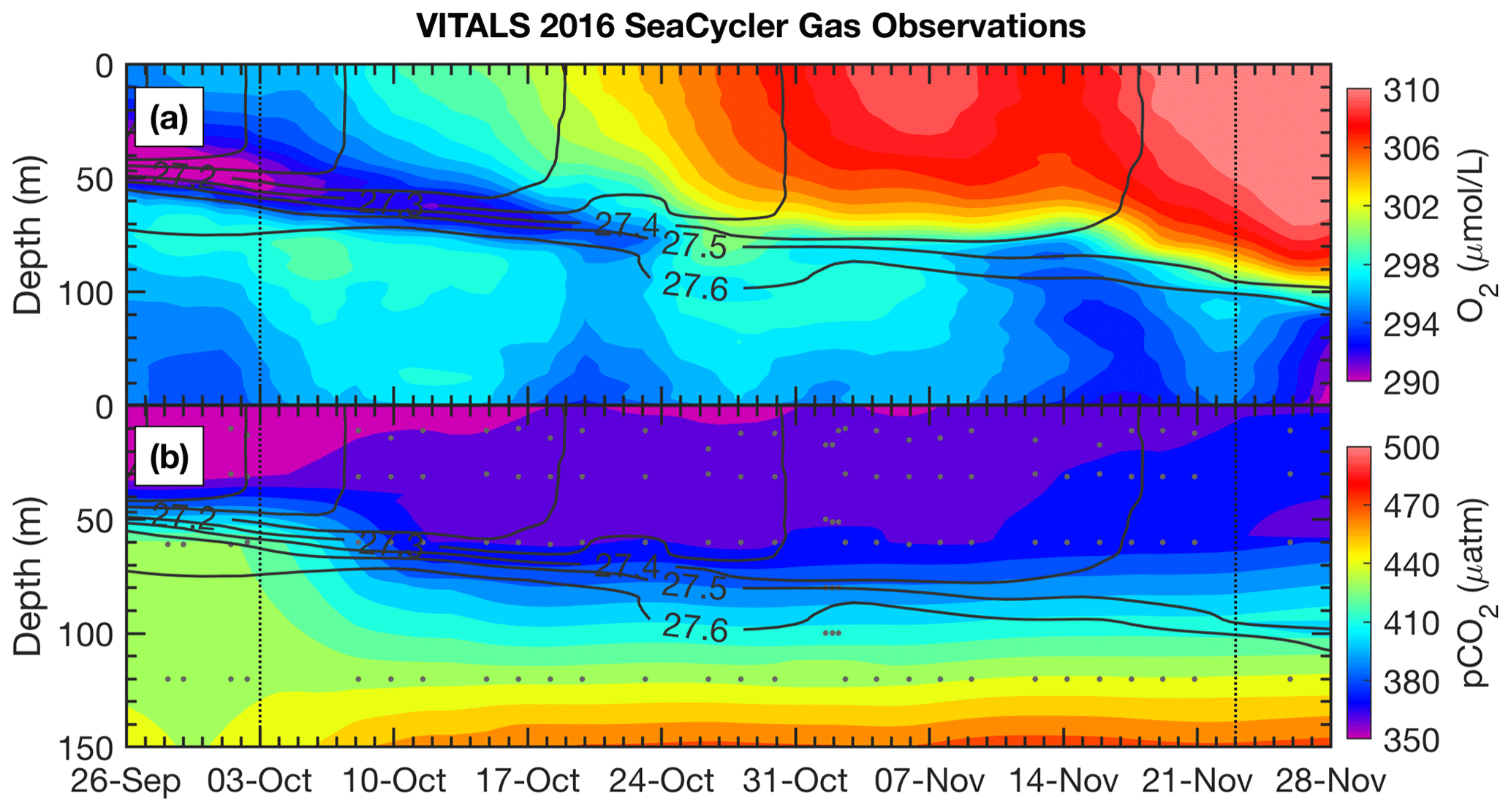
Figure 5 SeaCycler time evolution of (a) O₂ and (b) pCO₂ observations for the joint glider–SeaCycler sampling period with isopycnal anomaly contours overlaid (0.1 kg m⁻³ spacing). Small grey dots are the depth and time of discrete CO₂-Pro CV measurements by the SeaCycler. Vertical dotted lines indicate the start and end of the joint sampling period.

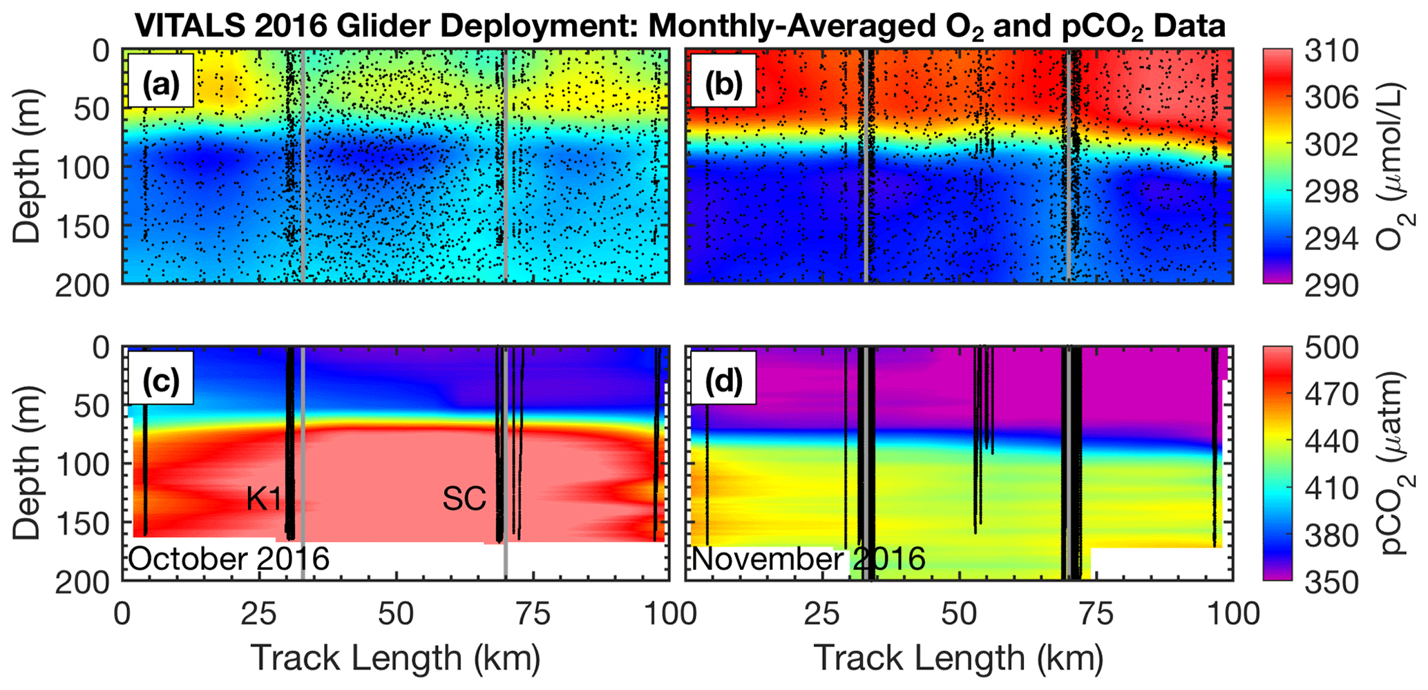
Figure 6 Glider monthly averaged spatial section of (a) O₂ in October and (b) November as well as for pCO₂ in panels (c) and (d), respectively (along-track positions are shown in the blue inset map in Fig. 1). Along-track locations of the K1 mooring and SeaCycler are indicated by vertical lines as are individual glider profiles used for plotting. For glider O₂ data only every 25th data point is shown for clarity.

Table 3 SeaCycler–glider residuals.

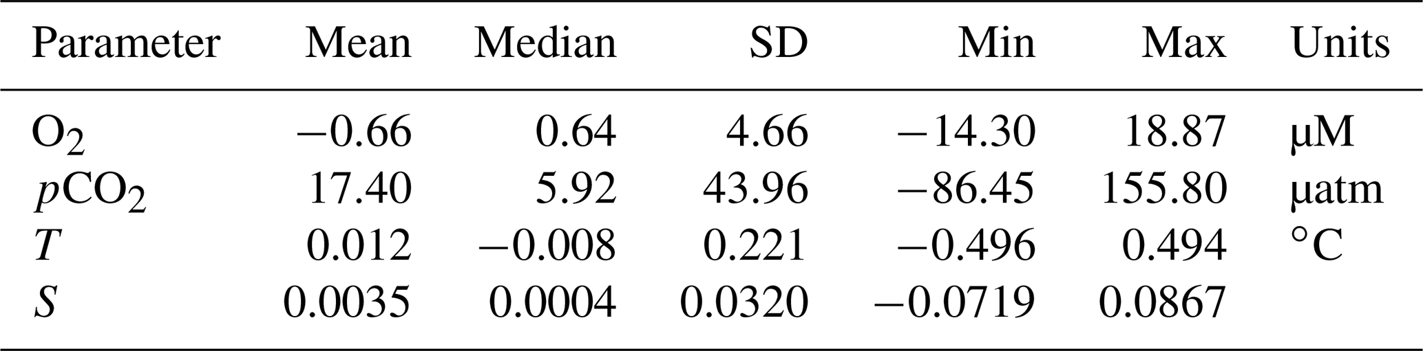
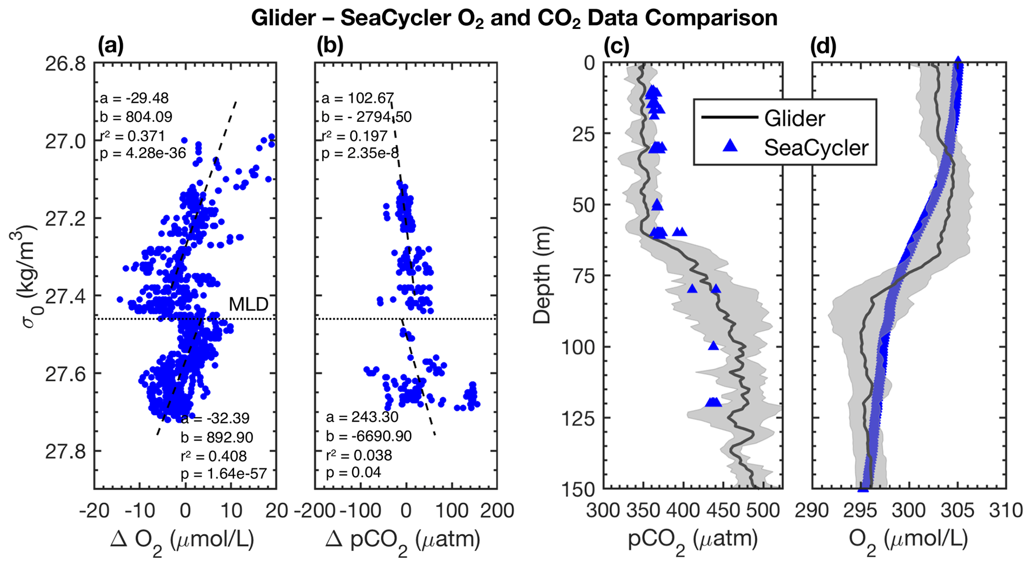
Figure 7 Glider–SeaCycler (a) O₂ and (b) pCO₂ isopycnal-matched residual comparison. Panels (c) and (d) show glider–SeaCycler-corrected depth-averaged pCO₂ and O₂ values with the glider 95 % CI shown as grey shading for the period from 3 October to 22 November 2016. Blue triangles are the mean of SeaCycler measurements for the glider observing period. The dashed horizontal line in panels (a) and (b) is the average density of the mixed layer, and the dashed lines are linear least-squares fits to the residuals in density space.

We intercompare platform observations and compute an in situ reference point for the glider data from the SeaCycler. For the comparison, we only consider data with similar T–S properties using isopycnal matching. We use the glider and SeaCycler data from the joint observing period (3 October to 22 November), binning data across potential density (σ₀) bins of 0.01 kg m⁻³ to compute the temperature and salinity residuals from both datasets. If temperature matched to within 0.5 ^∘C and salinity to within 0.1, we allowed these residuals for further comparison of O₂ and pCO₂ between platform observations. The 95 % confidence interval (CI) is defined as CI $=\stackrel{\mathrm{‾}}{x}$ ± 1.96 SD, where $\stackrel{\mathrm{‾}}{x}$ is the average of the variable of interest (e.g., pCO₂) and SD is the sample standard deviation. From the matching O₂ and CO₂ data, we plot the residual point cloud across the potential density anomaly. We find a strong duality in residual trends marked by the 27.46 kg m⁻³ isopycnal, coinciding with the average mixed layer depth (MLD) defined by a density difference criterion of 0.01 kg m⁻³ with respect to the surface (10 m). We use linear least-squares fits to compute the mean correction of the glider data required to match the SeaCycler (Fig. 7), indicating trends above and below the 27.46 kg m⁻³ isopycnal. Significant scatter (±50 µatm) is observed in CO₂ residuals below the mixed layer. Applying the residual fits from the SeaCycler–glider CO₂ offsets to the glider data as an in situ reference (Fig. 7c), we see reasonable agreement in the mixed layer. Below the mixed layer, the comparison does not fall within the 95 % CI limit. However, we see good agreement and relatively little spread (within ± 10 µM) of O₂ data between SeaCycler and glider sensors, leading to a good in situ reference. We observe that the mean (−0.66) and median (−0.64) offsets for O₂ are close compared to the mean (17.40) and median (5.92) offsets for pCO₂. Using the mean and standard deviation of the residuals and the SeaCycler's uncertainty (± 4.17 µM and ± 2 µatm), we estimate the mean offset and uncertainty for glider O₂ and pCO₂ data as −0.66 ± 6.14 µM and 17.39 ± 44.01 µatm, respectively.

3.3 Glider-observed spatial and temporal variability

Glider-based observations intrinsically link the spatial and time domain, making it hard to differentiate between these two dimensions. In VITALS, we took the approach of doing repeat glider sections along the same trajectory to capture both the time and spatial evolution of O₂ and CO₂ above and below the mixed layer. A Hovmöller diagram (Fig. 8) is useful to look at the propagation of processes across a time- and space-varying field.

We are interested in how much variability in O₂ and pCO₂ is captured by the SeaCycler time series data along the trajectory sampled by the glider when applying the residual fits from Fig. 7 to the glider data. Because the in situ comparison between the glider and SeaCycler CO₂ data was better at the surface, we only consider data within the mixed layer (0–20 m). We compute surface O₂ and pCO₂ anomalies with respect to the SeaCycler by subtracting corresponding SeaCycler surface daily averaged data from the glider record. We use the objective interpolation technique described earlier, interpolating the data using an exponential weighting function to fill in gaps along a 50 d (3 October–22 November) and 100 km grid. We could have used linear interpolation for the glider oxygen data but decided to keep mapping methods consistent between O₂ and pCO₂ data. A drawback of this technique is that it can show artificial variability in the resultant interpolated surface. We applied a low-pass filter, removing signals shorter than 3 d (time of glider transect) and 4 km (average distance between dives). We used larger scales of 40 km for the glider pCO₂ data. Dots indicate the location of data samples.

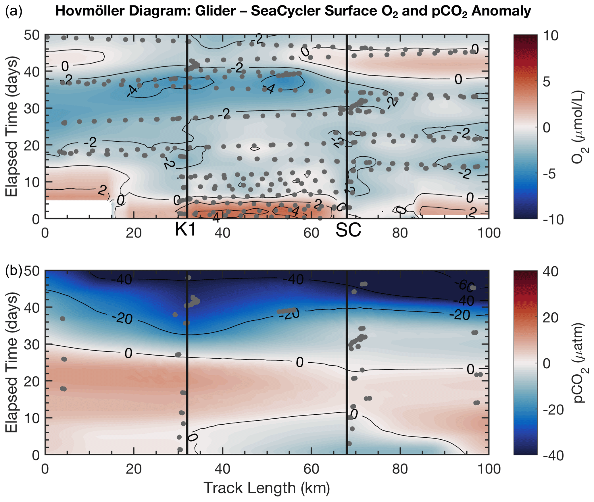
Figure 8 Glider Hovmöller diagram for O₂ (a) and pCO₂ (b) surface-averaged data (0–20 m) with SeaCycler data removed for the period 3 October–22 November 2016. Dots indicate the location of data samples. The location of K1 and SeaCycler (SC) moorings is shown in black.

Figure 8 shows the spatial and temporal anomalies of the glider data referenced to the SeaCycler data. We note that the scales of the anomalies are within the estimated uncertainty of the glider data. We see that only a few spatial features are visible in O₂ data, and the overall spatial structure is not as pronounced as the time variability. Towards the beginning of the record, there is a distinctly more oxygenated zone between the K1 mooring and SeaCycler. This could mean that the low oxygen levels measured by the SeaCycler from August to October had more considerable spatial variability. There are different patterns between moorings. Near the SeaCycler, the O₂ levels are elevated by 2 µM compared to the K1 mooring, while data near the K1 mooring show lower oxygen levels over time. Towards the second half of the glider record, as storm activity increases in November, the spatial domain becomes smoother with spatial variability reduced to ± 1 µM. The glider sampled O₂ daily and along the entire track length, while the CO₂ optode was only sampled at select locations on average every 2–3 d. The CO₂ glider data sampling was too sparse and required too much smoothing to resolve signals smaller than the seasonal cycle. Therefore, the data appear very uniform along the track length. However, this type of direct comparison between platforms will become increasingly important, especially as sensor improvements improve data accuracy. For future glider deployments, this approach may also help to achieve long-term monitoring capability through recalibrating sensors that suffer from drift and help with quality control of mobile platform data.

To separate temporal and spatial variability from each other, we can treat each dimension independently by comparing their autocorrelation scales against each other to measure the variability observed. For this analysis, we did not include the glider observations of CO₂ due to the sparse sampling across space and time. However, the scales that drive variability in T, S, and O₂ data also affect the dynamics of CO₂ solubility and the extent and strength of carbon sinks (Li et al., 2019; Atamanchuk et al., 2020). We use the definition from Chatfield (1998) of the correlogram or autocorrelation r(k) as a function of lag k.

$$\begin{array}{}\text{(3)}& r\left(k\right)={\displaystyle \frac{{\sum }_{t=\mathrm{1}}^{N-k}(x_t-\stackrel{\mathrm{‾}}{x})(x_{t+k}-\stackrel{\mathrm{‾}}{x})}{{\sum }_{t=\mathrm{1}}^N(x_t-\stackrel{\mathrm{‾}}{x}{)}^{\mathrm{2}}}}\end{array}$$

Here, x_t denotes any quantity of interest (e.g., T, S, or O₂), $\stackrel{\mathrm{‾}}{x}$ is the average of x_t along dimension t, k can denote either spatial or temporal lags, and N is the total number of samples along each dimension. We detrended the gridded space–time glider data to remove nonstationary time and spatial trends following Chatfield (1998) and computed the autocorrelation in space and time lags (kilometers and days) for S, T, and O₂. We repeat this analysis across the potential density anomaly contours of 27.3, 27.7, and 27.75 kg m⁻³, corresponding to the surface, intermediate, and deepest water regions surveyed by the glider. We include this analysis in the 95 % CI bounds defined previously as CI $=\stackrel{\mathrm{‾}}{x}$ ± 1.96 SD, where SD is computed from the range of correlation functions calculated for the whole isopycnal glider space–time dataset.

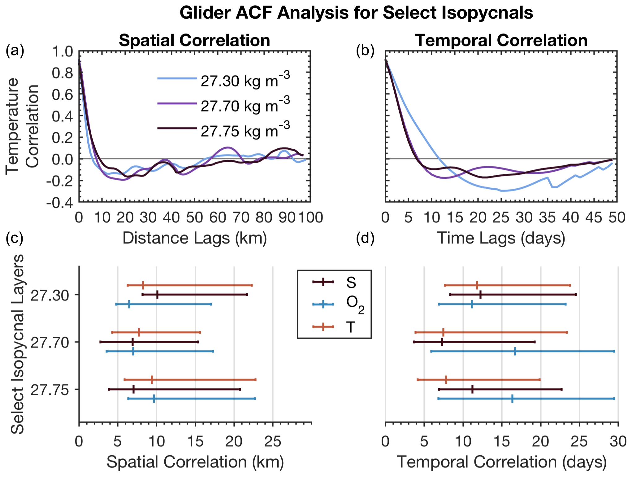
Figure 9 Upper panels show example autocorrelation functions for T as a function of distance and time lags. Lower panels summarize zero crossings for T, S, and O₂ in space and time lags for shown isopycnals together with 95 % CI bounds.

The autocorrelation function for T, S, and O₂ (Fig. 9) shows different spatial scales and timescales across all properties between surface and deeper water layers. T, S, and O₂ have similar spatial first zero crossings of approximately 7–10 km for intermediate and deep waters (27.7–27.75 kg m⁻³). O₂ and T also have similar scales (6–7 km) for surface mixed layer waters (27.3 kg m⁻³). S has the first zero crossings at scales around 10 km at the surface mixed layer. CI limits on T and O₂ are more similar in intermediate-depth waters and differ at the surface, where T and S seem to be more closely related than oxygen. Across T, S, and O₂, the CI limit is constrained by 23 km on the upper end and 3 km on the lower end.

Timescales vary more between properties than do spatial scales. T, O₂, and S have similar temporal correlation at the surface (11–13 d). On the other hand, O₂ has very different intermediate-depth scales (16 d) compared to T and S (7–11 d). These results suggest that there are different underlying dynamics between the surface and intermediate–deep water layers that drive T, S, and O₂ timescales as observed in the temporal SeaCycler record (Fig. 5). The CI timescale limits for O₂ are also different compared to T and S in intermediate layers. The temporal scales for O₂ in the intermediate-depth layer fall within the mean of the CI interval (6–29 d), suggesting that the distribution of correlation values is centered around this range of scales. On the other hand, T and S scales are closer to the lower limit of the 95 % CI bounds (4–24 d).

Overall, spatial scales vary less dramatically between density layers than temporal scales. The presence of energetic shifting of density layers (every 3 to 5 h) in the intermediate-depth waters would force spatial scales to be small. The glider takes about 3 h to complete a full dive–climb cycle over a distance of 3–4 km. As the glider begins the next dive–climb cycle, the glider will likely see a shift in the depth of intermediate-depth density layers as it will be between 3 and 5 h since it first measured the same density layer. A study by Sathiyamoorthy and Moore (2002) found similar timescales of T and S of around 2 weeks at the surface, explaining the observed timescales from buoyancy fluxes observed in OWS Bravo data. They link correlation scales in T and S to cyclonic airflow regime changes in the North Atlantic, suggesting storm activity at roughly 2 weeks in the Labrador Sea in the fall. Their result indicates that storms occurring every few weeks are primarily responsible for changes in T, S, and O₂ in the surface layer.

The significant difference in timescales between T–S (7–11 d) and O₂ (16 d) across intermediate–deep layers, however, is not intuitive. Changes in O₂ may be related to biogenic activity with a 2-week period. However, this would not explain changes in T and S. We cannot be sure without further insights from direct observations into the fall and early winter in the Labrador Sea. The small spatial scales of around 10 km do suggest highly variable changes. Due to temperature dependence, this should also result in localized changes in CO₂ cycling. We still do not know exactly how much carbon is taken up in the Labrador Sea, and understanding the impact of localized changes to solubility pumps is an important step. Small-scale spatial variability of pCO₂ for CO₂ uptake is important. To distinguish the changes in the strength of CO₂ uptake, we need to continue to improve spatial observations of CO₂ concentrations in these regions.

We are aware that neither timescale nor spatial-scale results can be interpreted without being mindful of the glider platform's limitations due to aliasing (Rudnick, 2016) and the uncertainty of the collected data. However, compared to contemporary studies in other water regions, our scale results point to much higher variability across all properties, including CO₂ along time–space dimensions in the Labrador Sea. For reference, traditional annual ship sampling programs in the Labrador Sea, such as the AR7W section, cover the track of the whole glider mission in a fraction of time but have spatial gaps on the order of tens of nautical miles between stations – well above the average spatial correlation length scales observed by our glider mission. Other platforms such as Argo floats cover larger areas but lack the glider platforms' targeted sampling capability. Therefore, gliders play an important role in constructing an effective observing strategy to resolve the fine-scale processes missed by other platforms.

4 Conclusions

In this study, we show data and results of testing a pCO₂ optode sensor (Aanderaa model 4979) on a glider. However, improving glider-based CO₂ observations is essential to capture the evolving space–time dynamics of carbon sinks in the ocean. We addressed three questions in this paper. (1) How suitable is the novel CO₂ optode for glider-based applications? (2) How can multiple autonomous platforms be used to help improve sensor data? (3) How can combined moored and mobile platforms resolve scales of temporal and spatial variability? We view answering these questions as essential to advancing current sensor technology and glider-based CO₂-observing capabilities.

Our deployments were the first glider-based tests of the novel pCO₂ optode. We deployed the glider in an initial test as part of a mission to collect data between two moorings in the central Labrador Sea. From the evaluation of the first mission in the fall of 2016 in the Labrador Sea and questions about the performance of the CO₂ optode sensor during small temperature changes (<3 ^∘C over 100 m), we re-deployed the glider in Trinity Bay, Newfoundland, where vertical temperature differences are large (>10 ^∘C over 100 m). For the second test, we focused on extensive initial tank comparisons between the CO₂ optode and reference sensors using a large saltwater tank that allowed us to submerge all systems at once. We also attempted various glider missions such as the staircase mission vs. regular glider profiles to differentiate the sensor performance. Several difficulties in using the sensor on a glider were observed, such as drift and long response times. In both missions, the sensor foil conditioning effect is initially observed as a steep exponential curve, flattening after some time. In the VITALS mission, the sensor showed strong conditioning effects in the first cycle of the deployment and stabilized after about a month into the deployment. We calculated an initial conditioning offset of 1275 µatm by comparing the sensor data with atmospheric measurements and the SeaCycler. For the Trinity tests, the sensor stabilized after about 4 d (offset of 994 µatm), but the sensor showed a nonlinear depth-dependent response towards the end of the mission, and almost 2 d of data had to be excluded.

From the VITALS Labrador Sea deployment, we calculated average response times (τ₉₅) of the sensor of 169.8 ± 186.6 s for temperature gradients of 0.22 ± 0.58 ^∘C. In Trinity Bay, with larger temperature gradients of 2.70 ± 5.62 ^∘C, we find response times are 99.2 ± 45.2 s. We were able to correct the sensor's response time by applying methods similar to those in Fiedler et al. (2013). However, more tests are required to validate our results and characterize the influence of other factors, such as the boundary layer in the sensor's flow field. We identified a large scatter in sensor response times for small temperature gradients in the Labrador Sea data. We also detected a small bias in performance towards positive temperature gradients, suggesting the sensor performs better in upcasts than in downcasts. Presently the sensor does not yet have the reliability to measure pCO₂ from a glider. The sensor's drift and conditioning are not well understood, and not many prior published test results are available for comparison. The sensing foil likely needs more work to improve stability. The optode has some key strengths, such as its small size, easy integration, and low power consumption. If the foil stability and sensitivity could be improved, the sensor could become a desirable candidate for ocean gas measurements similar to the commonly used O₂ optode.

In the Labrador Sea mission, we demonstrated how to use the SeaCycler CO₂-Pro CV instrument as an in situ mid-deployment reference point to validate the glider CO₂ data. Our corrections for the experimental glider CO₂ optode, using SeaCycler data, yielded a robust surface mixed layer correction of the glider data, but the subsurface data remained noisy. For the more reliable O₂ optode, this method worked well, and agreement in data to within ± 10 µM was achieved. Using the residuals from the glider–SeaCycler comparison, we estimate the mean offset and uncertainty for glider O₂ and pCO₂ data as −0.66 ± 6.14 µM and 17.39 ± 44.01 µatm, respectively.

The unique capability to synchronize and synthesize data from different sensor systems allowed us to investigate the high-resolution glider observations' spatial and temporal character. The repeat sections of the glider yielded a dynamic picture across all measured properties (T, S, O₂, CO₂) in both time and space. On average, we observed spatial scales across measured properties of less than 10 km and temporal scales of 15 d or less. Our results agreed with previous studies, pointing to increased storminess in the fall to explain the roughly 2-week period in timescales. We lacked enough data to also quantify timescales and spatial scales of pCO₂. However, given the strong dependence between T and CO₂, our results point to the importance of having targeted wintertime glider observations to observe small-scale spatial variability of CO₂ cycling. Overall, our analysis points to much finer-scale and more localized processes than commonly described in the literature or captured by other observing systems, underlining the importance of repeat glider observations in this region.

These results clearly show that challenges remain to achieve reliable glider-based CO₂ observations. The CO₂ optode sensor does not yet meet the targets for ocean acidification observations, as discussed by Newton et al. (2015). In the meantime, one option is to measure pH rather than CO₂. The work by Saba et al. (2018), testing an ISFET pH sensor on a Slocum glider, found accuracy to be better than 0.011 pH units and is indeed very promising. These sensors are already in regular use on BGC Argo floats. Calculation of pCO₂ from pH requires knowledge of at least one other carbonate parameter. On the other hand, pH vs. pCO₂ relationships measured at fixed platforms like the SeaCycler could support this calculation. One limitation of the pH sensor is that one could not use the data to measure air–sea gas exchange because it is not a direct measurement of pCO₂. No matter which sensor one chooses, we believe that in situ referencing between platforms can add value to existing and future sensors deployments on autonomous platforms such as floats, gliders, and moorings.

Appendix A: DFO sample analysis

Niskin bottle samples were collected in the lab in 500 mL biological oxygen demand (BOD) bottles. They were poisoned using 100 µL of saturated mercuric chloride (HgCl₂) and allowed to warm in a temperature-controlled bath (25^∘C ± 0.1 ^∘C) before analysis. Winkler titrations were performed on water samples to calculate oxygen concentrations. Uncertainties of the Winkler titrations were ± 0.01 mL L⁻¹ or ± 0.44 micro-molar (± 1 SD). A_T and DIC were estimated from coulometry (Johnson et al., 1993) and potentiometric titration (Mintrop et al., 2000). Equipment used to estimate A_T and DIC was as follows: VINDTA 3D A_T–DIC analyzer connected to a coulometer (UIC, USA, model 5015O) and VINDTA 3S (A_T) analyzer using open-cell differential potentiometry equipped with a reference (Metrohm, Canada, model 6.0729.100) and pH glass (Thermo-Orion, Canada, model 8101BNWP Ross half-cell) electrode, which were both referenced against a grounded platinum electrode. Based on A_T and DIC, pCO₂ was calculated using CO2calc (Robbins et al., 2010) with CO₂ equilibrium constants (Mehrbach et al., 1973; Dickson and Millero, 1987), a total boron constant (Lee et al., 2010), and KHSO4 constants (Dickson, 1990). Analytical instrumentation at DFO undergoes a daily operational evaluation of accuracy using certified reference materials (CRMs), from which estimated uncertainty for DIC and A_T measurements are 3 and 4 µmol kg⁻¹, respectively (Gary Maillet, personal communications, 2020). Including the A_T–DIC input uncertainty in CO2calc, we estimate pCO₂ uncertainty as ± 4.48 µatm.