Global sea level reconstruction for 1900–2015 reveals regional variability in ocean dynamics and an unprecedented long weakening in the Gulf Stream flow since the 1990s

A new monthly global sea level reconstruction for 1900–2015 was analyzed and compared with various observations to examine regional variability and trends in the ocean dynamics of the western North Atlantic Ocean and the US East Coast. Proxies of the Gulf Stream (GS) strength in the Mid-Atlantic Bight (GS-MAB) and in the South Atlantic Bight (GS-SAB) were derived from sea level differences across the GS. While decadal oscillations dominate the 116-year record, the analysis showed an unprecedented long period of weakening in the GS flow since the late 1990s. The only other period of long weakening in the record was during the 1960s–1970s, and red noise experiments showed that is very unlikely that those just occurred by chance. Ensemble empirical mode decomposition (EEMD) was used to separate oscillations at different timescales, showing that the low-frequency variability of the GS is connected to the Atlantic Multi-decadal Oscillation (AMO) and the Atlantic Meridional Overturning Circulation (AMOC). The recent weakening of the reconstructed GS-MAB was mostly influenced by weakening of the upper mid-ocean transport component of AMOC as observed by the RAPID measurements for 2005–2015. Comparison between the reconstructed sea level near the coast and tide gauge data for 1927–2015 showed that the reconstruction underestimated observed coastal sea level variability for timescales less than ∼5 years, but lower-frequency variability of coastal sea level was captured very well in both amplitude and phase by the reconstruction. Comparison between the GS-SAB proxy and the observed Florida Current transport for 1982–2015 also showed significant correlations for oscillations with periods longer than ∼5 years. The study demonstrated that despite the coarse horizontal resolution of the global reconstruction (1^∘ × 1^∘), long-term variations in regional dynamics can be captured quite well, thus making the data useful for studies of long-term variability in other regions as well.

1 Introduction

Various analyses of tide gauge data show an acceleration of global sea level rise over the past century with particularly high rates of rise over the most recent years (Church and White, 2006, 2011; Merrifield et al., 2009; Jevrejeva et al., 2008; Woodworth et al., 2011; Hay et al., 2015; Dangendorf et al., 2017, 2019). However, the presence of pronounced natural variability at various timescales makes the detection of the long-term acceleration due to anthropogenic climate change more difficult with existing sea level data (Kopp, 2013; Dangendorf et al., 2014; Haigh et al., 2014; Kenigson and Han, 2014). Evaluating global sea level acceleration is important for understanding the global climate system, but knowing the mean global sea level rise is insufficient for the preparation of coastal communities under threat of increased flooding. Other factors such as land subsidence and ocean and atmospheric dynamics can have a significant impact on regional relative sea level rise, introducing substantial differences to global sea level rise (Cazenave and Cozannet, 2014).

The US East Coast is a region that has been recently labeled as a “hotspot for accelerated sea level rise” (Boon, 2012; Ezer and Corlett, 2012; Sallenger et al., 2012; Kopp, 2013; Ezer, 2013; Ezer et al., 2013; Gehrels et al., 2020). Land subsidence associated with the Glacial Isostatic Adjustment (GIA) plus local geological, cryospheric and hydrological processes increase local sea level rise along the US East Coast relative to the global rates (Boon, 2012; Kopp, 2013; Miller et al., 2013; Frederikse et al., 2017; Gehrels et al., 2020). An additional factor, less understood, is acceleration and deceleration due to the dynamic response to changes in ocean circulation; for example, a potential slowdown in the GS and AMOC (which the GS is part of) can increase coastal sea level along the western North Atlantic coasts (Ezer and Corlett, 2012; Sallenger et al., 2012; Ezer et al., 2013; Ezer and Atkinson, 2014; Rahmstorf et al., 2015; Little et al., 2019). Therefore, it is important to study regional climatic changes for flood-prone coastal communities. The idea of connections between weakening in the GS strength and rising coastal sea level is not new (Montgomery, 1938; Blaha, 1984) and has been identified in data and ocean models (Ezer, 1999, 2001, 2013, 2015; Ezer et al., 2013; Levermann et al., 2005; Yin and Goddard, 2013; Goddard et al., 2015). Because sea level is lower on the onshore side of the GS and higher on the offshore side (by ∼ 1–1.5 m; due to the geostrophic balance), changes in the path and strength of the GS offshore can impact coastal sea level variations along the US East Coast (see, e.g., Fig. 2 in Ezer et al., 2013). This connection involves various temporal and spatial scales and complex mechanisms, so detecting the exact connections between changes in the AMOC and the GS and coastal variability is still ongoing research (e.g., Little et al., 2019; Piecuch et al., 2019). The processes that transfer large-scale open-ocean signals to coherent regional coastal sea level response involve fast-moving barotropic ocean waves, slow-moving baroclinic waves and coastally trapped waves (Huthnance, 1978; Ezer, 2016; Hughes et al., 2019). Variations in the GS flow and path have a wide range of timescales: daily, mesoscale, seasonal, interannual, decadal, and multi-decadal or even longer. However, since direct continuous observations of the GS are relatively short, about 3 decades of satellite altimeter data and about 4 decades of cable observations of the Florida Current (Baringer and Larsen, 2001; Meinen et al., 2010), it is difficult to study past decadal and multi-decadal variability in ocean dynamics and compare it to current and future climate change. For example, limited past temperature and salinity ship observations and simple diagnostic numerical ocean models suggested that a dramatic decline of ∼30 % in the GS transport happened between the 1960s and 1970s (Levitus, 1989, 1990; Greatbatch et al., 1991); in the same period, an increase in sea level along the US East Coast of 5–10 cm was observed (Ezer et al., 1995). These changes in the 1960s and 1970s resemble recent changes (i.e., coastal sea level rise during periods of GS weakening), but direct observations of the GS and AMOC were not available at the time to allow comparisons with recent changes. Using ocean models forced by surface observations since the 1960s, Blaker et al. (2014) found similarities between the extreme minimum in AMOC in 2009–2010 and a similar minimum in 1969–1970, but this approach has some shortcomings due to model errors and lack of accurate surface forcing for earlier years.

One approach to overcome the above limitations of studying long-term past changes is to take advantage of the global coverage of recent altimeter data and combine these data with sparse, but long, tide gauges to obtain global sea level reconstructions. Various optimization and spatial analysis methods were used to produce global reconstructed sea level (Church et al., 2011; Calafat et al., 2014; Hamlington et al., 2014; Hay et al., 2015; Dangendorf et al., 2019). Here, we used the latest hybrid reconstruction of Dangendorf et al. (2019) (see more details in the next section), since it contains both spatial and temporal variability, as well as long-term trends in sea level. Note that this monthly global reconstruction excludes nonclimatic land motion, excludes seasonal cycles and is currently available at 1^∘ × 1^∘ resolution for 1900–2015 (future improvements assimilating higher-resolution ocean models, newly digitized tide gauge data and an extended period are planned). Dangendorf et al. (2019) used this reconstruction to study global sea level acceleration and the influence of Southern Hemisphere winds on sea level, while Gehrels et al. (2020) used it to study past sea level rise hotspots along the western North Atlantic Ocean coasts and their relation to the North Atlantic Oscillation (NAO) and to Arctic ice melt. The main goal here is to evaluate the usefulness of this reconstruction to study processes of long-term regional ocean dynamics. The western North Atlantic Ocean was chosen as a test case because of the important role that the GS and AMOC play in the basin's dynamics and the fact that the nearby coasts are considered “hotspots” for sea level rise, as described above. Some questions that the study addresses include the following: (1) can a coarse-resolution reconstruction that does not resolve sharp fronts like that of the GS be able to capture dynamic variations in a western boundary current? (2) How well does the reconstruction, which relies on a relatively short period of altimeter data and sparse tide gauge data, compare with recent independent observations of Atlantic Ocean circulation features such as the AMOC and the Florida Current? (3) What characterizes the long-term variability of sea level and ocean dynamics? In particular, it is important to assess how recent weakening in the AMOC is compared with past changes over the last century.

The paper is organized as follows: first, the data and the analysis methods are described in Sect. 2. Then in Sect. 3 the regional and global trends are compared, the reconstruction is evaluated against observations and decadal variations are studied. Finally, in Sect. 4, a summary and conclusions are offered.

2 Data sources and analysis methods

The global reconstructed sea level (RecSL) record (1900–2015) analyzed here is described by Dangendorf et al. (2019). This RecSL is a hybrid reconstruction based on 479 tide gauge records, satellite altimeter data and several geophysical ancillary datasets of contributing processes (e.g., gravitational, rotational and deformational effects of mass changes known as “fingerprints”, ocean circulation models, and GIA), combining the techniques of the Kalman smoother (Hay et al., 2015), optimal interpolation and empirical orthogonal functions (Calafat et al., 2014) at different timescales. The result is a monthly sea level field on a (1^∘ × 1^∘) grid that includes both variability and trends (though the annual cycle was removed). The aim here is to examine this global dataset for its usefulness in studies of regional ocean dynamics. The western North Atlantic region is characterized by strong mesoscale variability, an intense western boundary current (the Gulf Stream) and important coastal impacts from climate change and sea level rise along the US East Coast. Therefore, it is a challenging task for a coarse-resolution reconstruction, which does not resolve mesoscale features, to accurately represent the regional dynamics. Figure 1 shows, for example, a comparison between the mean sea surface height (SSH) in the RecSL and the higher-resolution (1∕4^∘ × 1∕4^∘) AVISO satellite altimeter data (Ducet et al., 2000). While the RecSL captured the main circulation patterns in the North Atlantic Ocean, the coarse-resolution reconstruction is more noisy and underestimates spatial SSH gradients (note, however, that fronts in each monthly field are more defined than in the long-term mean field).

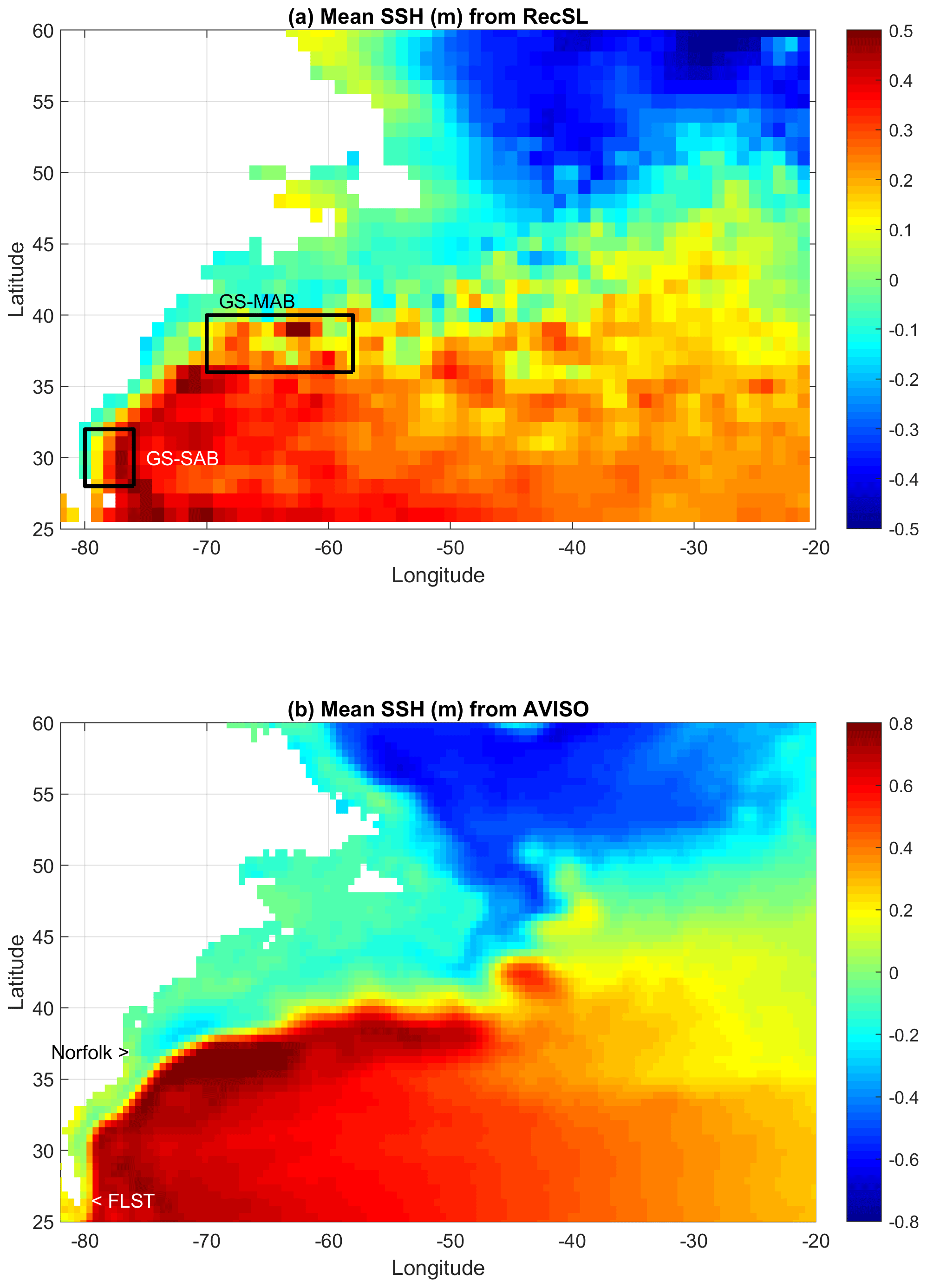
Figure 1 Mean sea surface height in the North Atlantic Ocean during the satellite era (1993–2015) obtained from (a) the RecSL reconstruction on a 1^∘ × 1^∘ grid and (b) the AVISO altimeter data on a 1∕4^∘ × 1∕4^∘ grid. Note the different color scale. The regions where the proxy Gulf Stream is defined in the Mid-Atlantic Bight (MAB) and the South Atlantic Bight (SAB) are marked in (a), and the location of the observations of the Norfolk sea level and the Florida Current transport at the Florida Straits (FLST) are marked in (b).

From the reconstructed sea level, a proxy of the GS strength was derived for two regions (Fig. 1a). Based on the assumption that the surface flow is close to geostrophic balance, the sea level gradient across the GS represents the strength of the surface GS. A shortcoming of this proxy is that it may not capture subsurface changes. In the Mid-Atlantic Bight (MAB), for each longitude the GS location is defined by the maximum north–south sea level gradient, so the averaged maximum gradient represents the mean eastward-flowing GS in the region (58–70^∘ W, 36–40^∘ N). The units are change in centimeters per 1^∘ latitude. In the South Atlantic Bight (SAB) similar latitudinal averaging of east–west gradients will represent the mean northward-flowing GS in the region (76–80^∘ W, 28–32^∘ N), i.e., between the Florida Strait and Cape Hatteras. These two proxies will be referred to as GS-MAB and GS-SAB, respectively.

The monthly mean sea level record (1927–2015) for the tide gauge station in Sewells Point near Norfolk (76.33^∘ W, 36.95^∘ N; Fig. 1b) was obtained from the Permanent Service for Mean Sea-level (PSMSL, http://www.psmsl.org, last access: January 2020; Woodworth and Player, 2003; Holgate et al., 2013). Since the RecSL record does not include seasonal variability (Dangendorf et al., 2019), the mean annual cycle was calculated and removed from the tide gauge data to allow a fair comparison. The Norfolk station at the southern end of the Chesapeake Bay was chosen because it is one of the US cities currently facing some of the largest impacts of sea level rise and increased flooding. This tide gauge record was subject to numerous studies that link coastal sea level there with changes in ocean dynamics (Ezer, 2001, 2013; Ezer and Corlett, 2012; Ezer et al., 2013; Ezer and Atkinson, 2014). While this tide gauge was part of the reconstruction, it is not completely independent from RecSL, so the hybrid reconstruction has been validated thoroughly using random independent unassimilated sites (see the Supplement in Dangendorf et al., 2019). There are so many tide gauges along the US East Coast that the inclusion or exclusion of a single site such as Sewells Point will have a negligible effect on the reconstructed fields.

The Atlantic Meridional Overturning Circulation (AMOC) data were obtained from the RAPID observations at 26.5^∘ N for 2005–2015, as described in various studies (https://www.rapid.ac.uk/, last access: January 2020; McCarthy et al., 2012; Srokosz et al., 2012; Smeed et al., 2014, 2018). The AMOC transport (given in Sverdrups; 1 Sv = 10⁶ m³ s⁻¹) is the sum of three components: (1) the upper mid-ocean transport obtained from observations of density changes across the Atlantic Ocean, (2) the Ekman transport estimated from wind stress data, and (3) the Gulf Stream transport obtained from cable measurements of the Florida Current across the Florida Strait. These three components of AMOC are provided twice daily, but they were used here only to calculate monthly averages.

The monthly Atlantic Multi-decadal Oscillation (AMO) index (Enfield et al., 2001) for 1900–2015 was obtained from NOAA (https://www.esrl.noaa.gov/psd/data/timeseries/AMO/, last access: January 2020); AMO represents variations in the sea surface temperature (SST) over the Atlantic Ocean. Long-term variations in sea level, such as a ∼60-year-long cycle, are thought to be influenced by AMO (Chambers et al., 2012), and correlations of AMO with patterns of sea level along the US and European coasts are often indicated (Ezer et al., 2016; Han et al., 2019).

Daily observations of the Florida Current (FC) transport at ∼27^∘ N (see Fig. 1b) for 1982–2015 were obtained from NOAA/AOML (http://www.aoml.noaa.gov/phod/floridacurrent/, last access: January 2020); the data are described by Baringer and Larsen (2001), Meinen et al. (2010), and many other studies. Monthly averaged values were calculated to allow comparisons with the RecSL record. Note that the FC data had a gap from October 1998 to June 2000. However, the EMD analysis (see below) as a sifting or filtering process (described below) can easily handle uneven sampling intervals and data gaps, so it can detect variations on timescales longer than the gaps; this has been experimentally tested for long tide gauge records (see Fig. 8 in Ezer et al., 2016).

A useful tool to analyze nonlinear time series is empirical mode decomposition (EMD; Huang et al., 1998; Wu et al., 2007), whereby a repeated sifting process decomposes records into a finite number of intrinsic oscillatory modes c_i(t) and a residual “trend” r(t). The number of modes depends on the record length and the variability of the data. Unlike regression fitting methods, the shape of the trend is not predetermined (i.e., the method is “nonparametric”). Each individual mode does not necessarily represent a particular physical process, but often a group of modes can be shown to relate to a known forcing (Ezer et al., 2013; Ezer, 2015). EMD decomposes the original time series into modes:

$$\begin{array}{}\text{(1)}& \mathit{\eta }\left(t\right)=\sum _{i=\mathrm{2}}^{N-\mathrm{1}}{c}_i\left(t\right)+r\left(t\right).\end{array}$$

In the EMD analysis output, mode 1 will be the original time series (η), modes 2 to N−1 are oscillating modes with different frequencies from high to low, and mode N will be the trend (r). Combining several low-frequency modes will be equivalent to a low-pass filter. Note that unlike spectral analysis, the frequency and amplitude in each mode are not constant, and thus the analysis can capture nonlinear changes, such as climatic changes in the amplitude of decadal variability. An improved version of the original EMD is ensemble EMD (EEMD; Wu and Huang, 2009) used here, whereby ensembles of simulations with white noise are averaged. Here, 100 ensemble members are used with white noise of 0.1 of the standard deviation (see Ezer and Corlett, 2012, and Ezer et al., 2016, for sensitivity experiments with EEMD parameters and error estimations). EEMD filters out unphysical modes and is more accurate for detecting real low-frequency variability (Kenigson and Han, 2014). All the calculations here use EEMD, though for simplicity the text refers to “EMD”. Note that the sum of the low-frequency modes plus the trend will be equivalent to a low-pass empirical filter that will have a lower number of degrees of freedom than the original time series. Therefore, when calculating confidence levels on correlations between EMD modes, the “effective sampling size” or “effective number of degrees of freedom” is estimated following the method suggested by Thiebaux and Zwiers (1984). In this method, autocorrelation is used to estimate the typical timescales of low-frequency EMD modes and then the confidence level is adjusted accordingly. Empirical testing showed, for example, that if the 116-year-long monthly RecSL record correlation coefficient of R=0.08 provides a 95 % confidence level (P≤0.05), obtaining the same confidence level for low-frequency modes with autocorrelation timescales of 2, 5 and 10 years will require R>0.25, 0.35 and 0.55, respectively. There have been discussions on the robustness of EMD in terms of accurately detecting multi-decadal variability and nonlinear trends in sea level records (Chambers, 2015). Therefore, to bolster the EMD-based correlation analyses between the GS proxy, FC transport and the AMO, we also applied a wavelet coherence analysis (Grinsted et al., 2004), with the results being presented in Appendix A.

3 Results

3.1 Regional and global sea level rise

Using the same reconstruction (RecSL) analyzed here, Dangendorf et al. (2019) found, in addition to substantial decadal variability, a significant and persistent acceleration in global mean sea level rise since the 1960s. They attributed the initiation of this recent acceleration to shifts in Southern Hemisphere wind patterns, driving changes in ocean circulation and increasing the ocean's heat uptake. In the western North Atlantic, some studies suggest that acceleration in sea level along the eastern coasts of North America may be related to a slowdown of the AMOC and GS (Leverman et al., 2005; Boon, 2012; Ezer and Corlett, 2012; Sallenger et al., 2012; Yin and Goddard, 2013; Caesar et al., 2018). Future projections from climate models consistently indicate a weakening AMOC (Cheng et al., 2013; Reintges et al., 2017), though with divergent associated sea level responses in different models (Little et al., 2019). Therefore, it is important to understand the AMOC–sea level connection and try to detect current and past changes from observations. Bingham and Hughes (2009), for example, suggested that every 1 Sv weakening in the AMOC could raise the sea level along the North American coast by ∼2 cm. To evaluate regional patterns in sea level rise, the sea level change in the southwestern North Atlantic for different periods was calculated (Fig. 2a–e) as was the sea level change for the entire record for 1900–2015 (Fig. 2f). Two findings emerge from this analysis: first, the sea level is rising at very different rates during different periods. For example, from 1915 to 1935 (Fig. 2a), the sea level rose in the southwestern North Atlantic region by ∼ 0.02–0.04 m (rate of ∼ 1–2 mm yr⁻¹; similar to the global rate seen in Fig. 2 of Dangendorf et al., 2019), while from 1995 to 2015 (Fig. 2e) the sea level in this region rose by ∼ 0.05–0.2 m (rate of 2.5–10 mm yr⁻¹). Therefore, there is clearly a faster sea level rise since the 1990s compared with previous periods (i.e., sea level rise acceleration), but the sea level rise is spatially very uneven (Fig. 2f). It also seems that due to decadal variability, some periods even experienced a decreasing rate of sea level rise (i.e., deceleration); for example, sea level rise from 1955 to 1975 (Fig. 2c) was slower than sea level rise for 1935–1955 (Fig. 2b). Second, the largest changes are seen near the GS around 35–40^∘ N, with additional changes on the rim of the subtropical gyre (the reduction in sea level difference between the center and edge of the subtropical gyre can be interpreted as a sign of weakening circulation). The total sea level change between the first and last 5 years of the RecSL record (Fig. 2f) shows a faster sea level rise north of the GS (red area) and a slower sea level rise south of the GS (blue area), thus indicating a potential weakening trend in the geostrophic surface flow of the GS; this prospect is investigated later. Variations in the NAO and AMOC can cause changes in the GS position and/or in broadening its front (Taylor and Stephens, 1998; Joyce et al., 2000; Smeed et al., 2018), which can also result in spatial variations in sea level rise as seen here. However, the 1^∘ × 1^∘ RecSL grid will not resolve most of the variability in the GS position (Fig. 1a), which nevertheless can be seen by the higher-resolution altimeter data (Fig. 1b; see also Fig. 1 in Ezer et al., 2013).

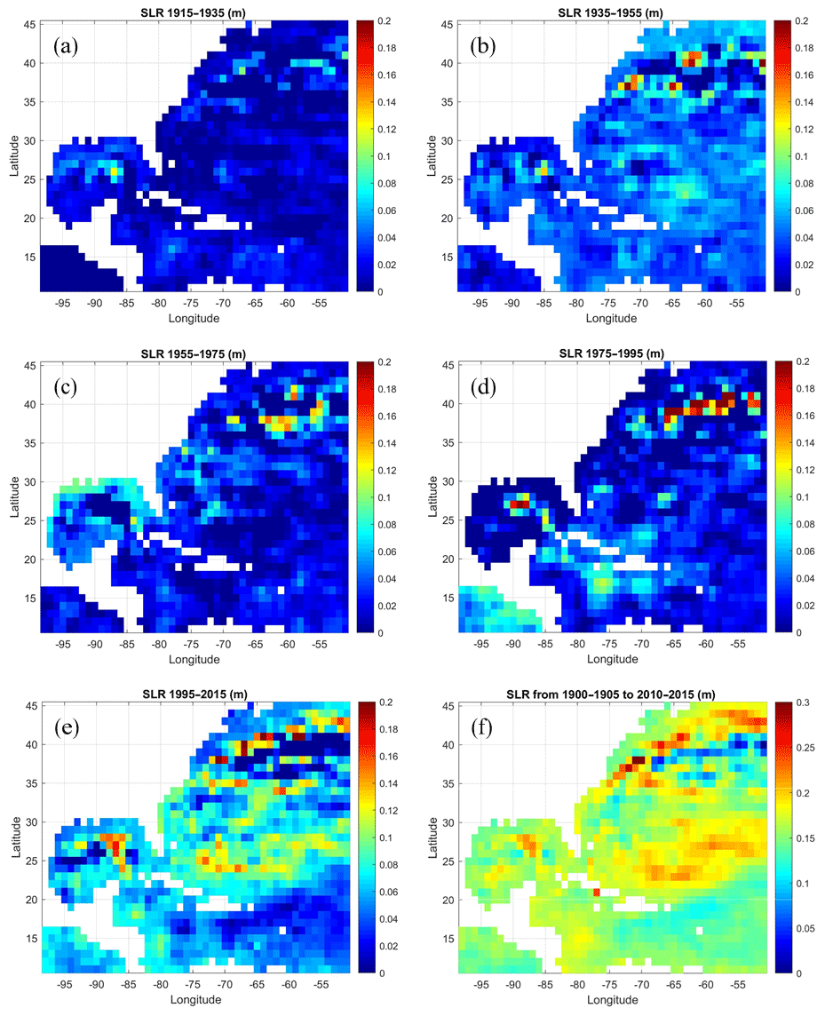
Figure 2 (a)–(e) Sea level change in different periods. (a) The difference between the mean sea level in 1915 and the mean sea level in 1935, (b) for 1935–1955, (c) for 1955–1975, (d) for 1975–1995 and (e) for 1995–2015. Note that the maximum sea level change in the color bar, 0.2 m per 20 years, is equivalent to a sea level rise of 10 mm yr⁻¹. (f) Sea level change between the first and last 5 years of the record (note the different color scale).

A comparison of the global monthly mean sea level with the regional mean sea level in the southwestern North Atlantic (the area shown in Fig. 2) indicates a similar general trend (Fig. 3a), but a much larger interannual and decadal regional variability of up to ±4 cm over the global mean sea level (Fig. 3b). Regionally, a lower than average sea level is seen in the 1920s–1940s, and a higher than average sea level is seen in the 1950s and 1980s. Low-pass-filtered data (Fig. 3b) show variations on two major timescales, periods of ∼ 5–10 years (the sum of EMD modes with periods longer than ∼5 years is shown in red) and ∼ 10–60 years (the sum of EMD modes with periods longer than ∼10 years is shown in blue). The decadal and multi-decadal variations in the global acceleration and deceleration of sea level were described by Dangendorf et al. (2019) and others, but we further want to evaluate here if regional variations in ocean dynamics may play a role and how these variations are connected to basin-scale climate modes (Han et al., 2019). Note that multi-decadal modes are not resolved by the satellite altimetry era, so low-frequency variations in the hybrid RecSL record are estimated by the Kalman smoother applied on the tide gauge records, while altimeter data contribute mostly to interannual to decadal variability (Dangendorf et al., 2019). We will return later to discuss the potential mechanisms behind the regional variability seen in Fig. 3b, but before that it is important to validate the RecSL record and evaluate its ability to capture observed the variability.

Figure 3 (a) Global mean sea level (black line) and regional mean sea level over the area shown in Fig. 2 (green line). (b) Difference between the monthly regional and global mean sea levels (green line). Heavy red and blue lines represent low-pass-filtered records obtained from the sum of EMD modes with timescales longer than ∼5 and ∼10 years, respectively.

3.2 Comparison of the reconstruction with recent data

Very few datasets are long enough to evaluate the entire 116 years of the reconstruction. However, various recent observations can be used to examine how well the global reconstruction can resolve regional and basin-wide dynamic processes. The focus here is on two types of observations: coastal sea level and the Florida Current.

3.2.1 Coastal sea level

The long tide gauge record (starting in 1927) at Sewells Point in Norfolk, VA (in the lower Chesapeake Bay), has been the subject of many studies due to the acceleration in flooding at this city (Boon, 2012; Ezer and Corlett, 2012; Ezer, 2013; Ezer and Atkinson, 2014); this location can be used to represent sea level variability in the MAB (Ezer et al., 2013). Note that due to the coarse resolution, the reconstruction completely omits the Chesapeake Bay. The reconstructed sea level also removes land subsidence, which is substantial in Norfolk (Boon, 2012; Ezer and Corlett, 2012; Kopp, 2013). Moreover, the altimeter data used in the reconstruction do not extend to the near-coast area or to rivers and bays, so comparisons between tide gauge data and altimeter data often show that small-scale and high-frequency variations in coastal sea level are not well represented in altimeter data, but interannual and decadal variations are captured quite well (see, e.g., Fig. 2 in Ezer, 2015). Therefore, a comparison of this tide gauge with the reconstruction (basically a 1^∘ × 1^∘ box offshore of the Chesapeake Bay) will indicate what portion of the coastal sea level variability has an origin in the offshore large-scale dynamic variability. Figure 4 shows that while interannual variations in the reconstruction are highly correlated with the tide gauge, variability in the reconstruction is only about one-half of the coastal observations. The correlation of ∼0.8 is generally consistent with comparisons made by Dangendorf et al. (2019) for other locations and may indicate that about 60 % of the coastal sea level variability is not locally generated within the bay area (at least for monthly data; hourly or daily data may have more influence from local atmospheric forcing and tides). The reconstruction may not evenly represent all timescales, so to examine this point the variability in the coastal sea level and in the reconstructed sea level is decomposed into EMD modes (Fig. 5). Cross-correlations help to identify the main oscillations in each mode. While statistically significant correlation (at 95 % confidence) is found at all modes (see Sect. 2 for details on confidence levels of EMD modes), the amplitudes of the variations are underestimated for high-frequency oscillations. In Fig. 6 the EMD modes of the observed and reconstructed sea level are compared. While the reconstruction captured the mean frequency of each observed mode almost perfectly (Fig. 6a), the variability of the reconstruction is underestimated by about a factor of 2 for the whole time series (mode 1) and for oscillations with periods $T<\sim \mathrm{5}$ years (Fig. 6b). The underestimation is likely due to the variability in the satellite altimeter data and not due to the reconstruction itself. For longer timescales (modes 7–10) the reconstruction captured the coastal variability extremely well, with correlations of ∼ 0.9–1. The lowest frequency of oscillating mode 10 in Fig. 5 is almost identical in the reconstructed and observed sea level, showing an apparent positive acceleration in sea level rise since the 1960s, in accordance with the global acceleration seen in Dangendorf et al. (2019). Modes 6–8 (with periods of 5–20 years) show especially strong oscillations (Figs. 5 and 6c). Note that much longer records are needed to study the oscillations of the lowest frequencies when only a few cycles are available, though unlike spectral analysis methods, the EMD method is able to detect the potential existence of very low-frequency modes, even from incomplete cycles.

Figure 4 (a) Comparison of the monthly observed coastal sea level (green line) at the tide gauge near Norfolk, VA (76.33^∘ W, 36.95^∘ N; see Fig. 1), and the reconstructed sea level (black line) in the closest 1^∘ × 1^∘ box near the coast. (b) Scatter plot of the data comparison. The trend and the seasonal cycle were removed from both time series.

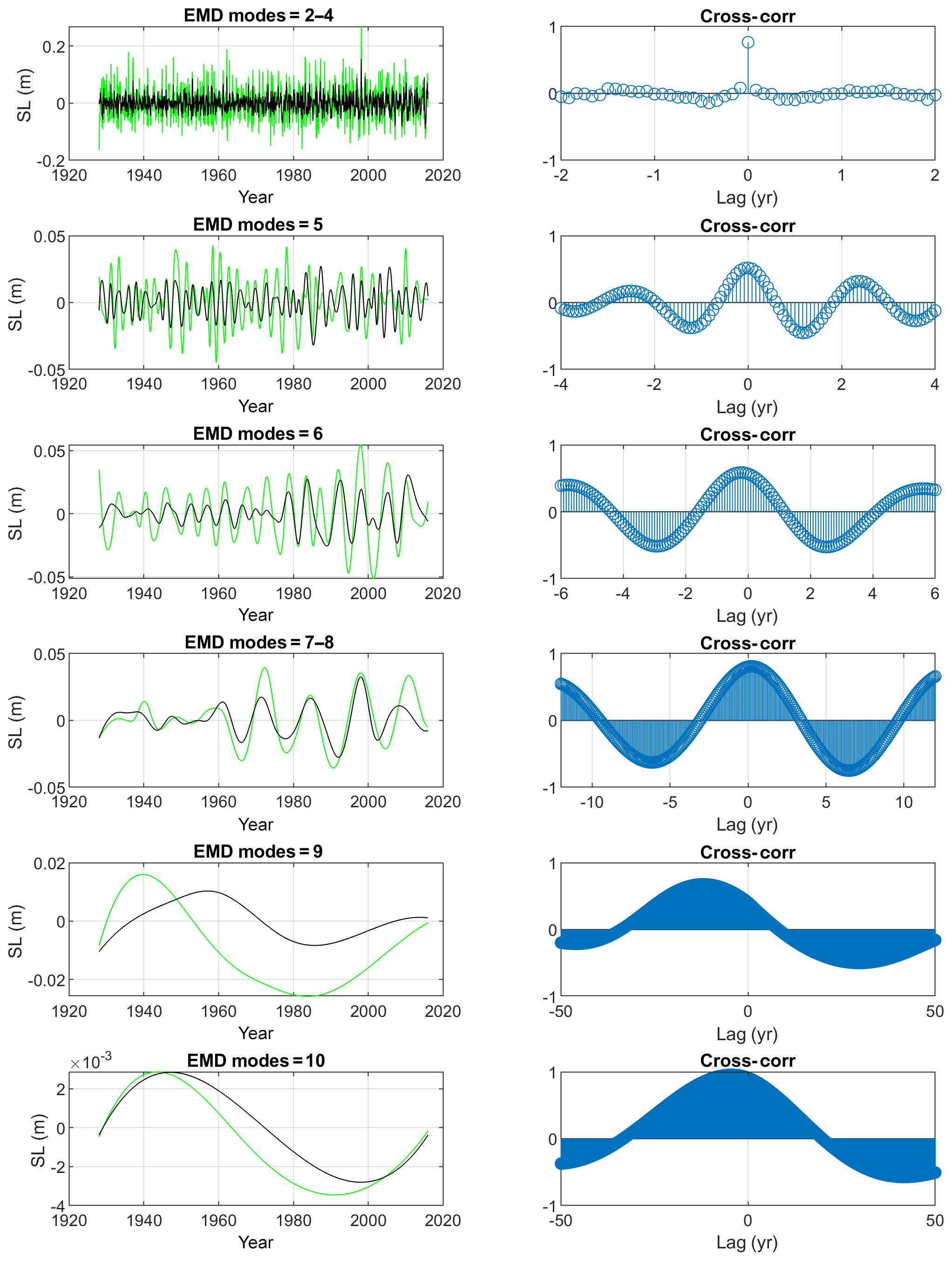
Figure 5 (left) EMD oscillating modes of the observed Norfolk sea level (green) and the reconstructed sea level (black). (right) Cross-correlation as a function of lag. High- to low-frequency modes are from top to bottom panels.

Figure 6 (a) Mean period of the EMD oscillating modes for the observed sea level (blue) and the reconstructed sea level (red). (b) Standard deviation of each EMD mode. (c) The cross-correlation between the observed and reconstructed sea level as a function of EMD modes and lag. Note that mode 1 is the original time series, modes 2–10 are oscillating modes (with time-dependent amplitude and frequency) and mode 11 is the trend.

3.2.2 The Florida Current (FC)

In Fig. 7 the observed FC transport for 1983–2015 is compared with the reconstructed GS proxy for the MAB and the SAB. Note that for this period, the FC shows a small weakening trend of −0.03 Sv yr⁻¹ (∼0.9 % per decade), while a larger recent weakening (∼1.5 % per decade) is seen during the RAPID/AMOC observations of 2005–2015 (see discussion in next section). The correlations of the FC with the GS proxy are larger in the SAB (R=0.58; Fig. 7b) where the GS is closer to the Florida Straits than in the MAB (R=0.28; Fig. 7a) where the GS is farther downstream from the observed FC (see Fig. 1). The lower correlation in the MAB (though statistically significant at 95 %) seems to be due to a phase lag between the upstream SAB and the downstream MAB. This incoherence between the GS and coastal sea level on the two sides of Cape Hatteras (i.e., the SAB versus the MAB) was investigated in several recent studies (Woodworth et al., 2016; Valle-Levinson et al., 2017; Domingues et al., 2018; Ezer, 2019). It is interesting to note that the relation between low-frequency changes in the FC transport and sea level as seen in Fig. 7b implies a ratio of about 1 Sv to 1.5 cm, while Bingham and Hughes (2009) suggested a ratio of ∼1 Sv to 2 cm between AMOC transport and coastal sea level.

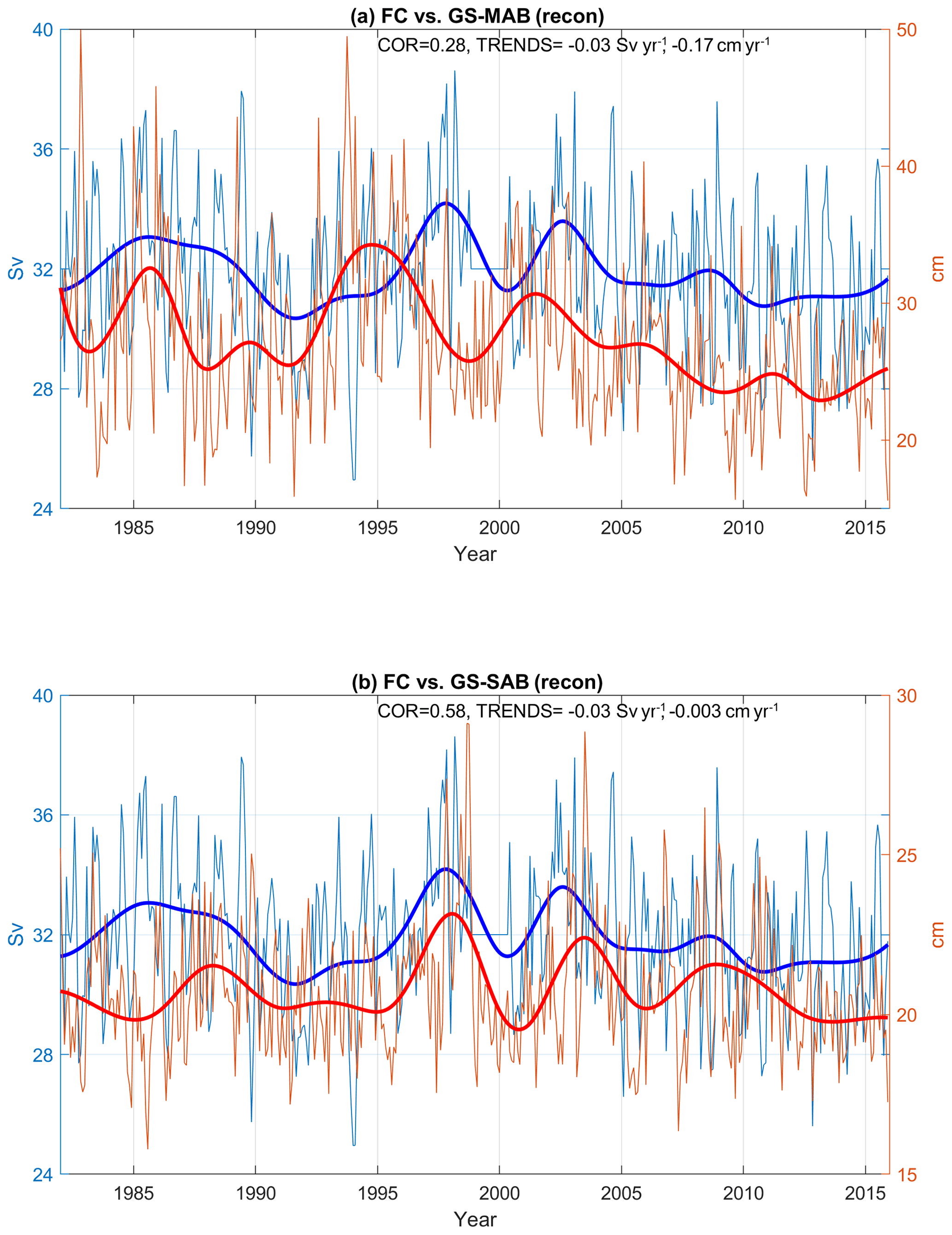
Figure 7 Comparisons between the observed monthly Florida Current transport (blue, in Sverdrup units on the left) and the GS proxy (red, in centimeter sea level change units on the right) obtained from the reconstructed sea level difference across the GS for (a) eastward velocity in the GS-MAB and (b) northward velocity in the GS-SAB. Thin lines are monthly values and, the heavy lines are low-pass-filtered records (sum of low-frequency EMD modes). The correlation of the low-frequency modes and the trends of the monthly records are indicated.

EMD analysis further compares the relationship between the GS-SAB proxy (derived from the east–west sea level difference) and the observed FC for different modes (Fig. 8). The high-frequency oscillations of the FC and the GS-SAB are not significantly correlated; in fact, oscillations for an approximately 2-year period show a small but nonsignificant anticorrelation at lag zero (second panels from the top in Fig. 8). However, variability on timescales longer than ∼5 years is highly correlated (R = 0.8–0.9 for modes 6–8 in Fig. 8), with the GS-SAB lagging behind the observed FC transport; this low-frequency variability in modes 6–8 represents cycles with periods of ∼5, ∼12 and ∼24 years, respectively (see right panels in Fig. 8). This result is further supported by a complementary wavelet coherence analysis (Appendix A, Fig. A1). While theoretically it is expected that sea level difference across the GS will be correlated with the FC, it is encouraging that a coarse-resolution global reconstruction on a 1^∘ grid that does not resolve the GS front very well can still capture the majority of the low-frequency variability of the FC. It is noted that although the reconstruction is based on satellite altimeter data that started in 1993, ocean dynamic variability in the 1980s, before the satellite age, is still captured quite well.

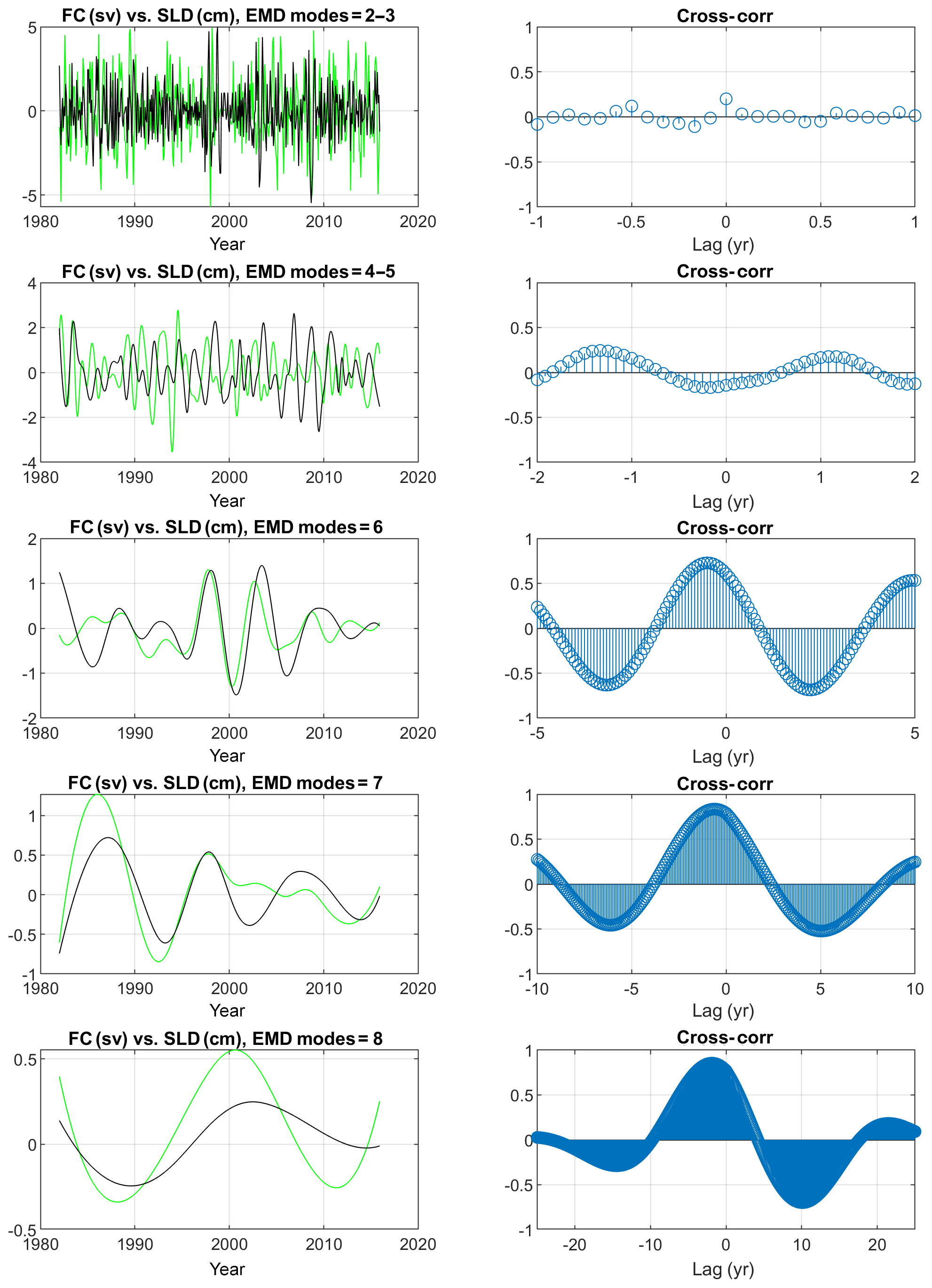
Figure 8 (left) EMD oscillating modes of the observed Florida Current transport (green, in Sverdrups) and GS-SAB proxy from the reconstructed sea level (black, in centimeters). (right) Cross-correlation as a function of lag. High- to low-frequency modes are from top to bottom panels.

3.3 Potential driving mechanisms for decadal variability in the RecSL

Variability in the GS-MAB proxy (obtained from sea level gradients as described in Sect. 2) is shown in Fig. 9a, indicating large variability on interannual and decadal timescales, with a persistent weakening trend since ∼1990 after a period of strengthening flow from the 1970s to the 1990s. The changes in the low-frequency oscillations are shown in Fig. 9b, indicating two long periods with declining GS strength (red area) during the 1960s and 1970s and after ∼1995, with maximum weakening of ∼25 % per decade. Recent observations by Andres et al. (2020) at 68.5^∘ W found the GS transport to be about 10 % weaker today than it was in the 1980s at the same location, but the same study also found a very large discrepancy in the trend between two sections located just a few hundred kilometers from each other; a western section from ship crossing showed no statistically significant trend (Rossby et al., 2014), and an eastern section from mooring data showed potential weakening of ∼ 5 % per decade to 10 % per decade. Based on altimeter data, Dong et al. (2019) and Zhang et al. (2020) also showed different trends between the eastern and western parts of the GS. Therefore, an average GS proxy over a large area as used here may filter out spatial variations; the RecSL record is also much longer than the altimeter data used in the above studies. The coarse resolution of the reconstruction also served as a filter that smoothed out small spatial variations and the impact from local recirculation gyres as seen in Andres et al. (2020). The GS-MAB proxy here shows that the recent weakening period is the longest in this record. To test if the long period of GS weakening is “unprecedented” or distinct from random natural variability, statistical analysis with 1000 simulations using random red noise (following an autoregressive process of the order of 1) imitating the spectrum of the record in Fig. 9a was performed, and the results are shown in Appendix A, Fig. A2. This analysis shows that obtaining long periods of weakening from random variability is extremely rare: in 116 000 years of artificial simulations there were only three cases of weakening of 10 % per decade that lasted for 10 years. For comparison, in the 116 years of reconstructed GS there were two such cases, with 10 % per decade weakening of ∼10 years in the 1970s and ∼15 years in the 2000s.

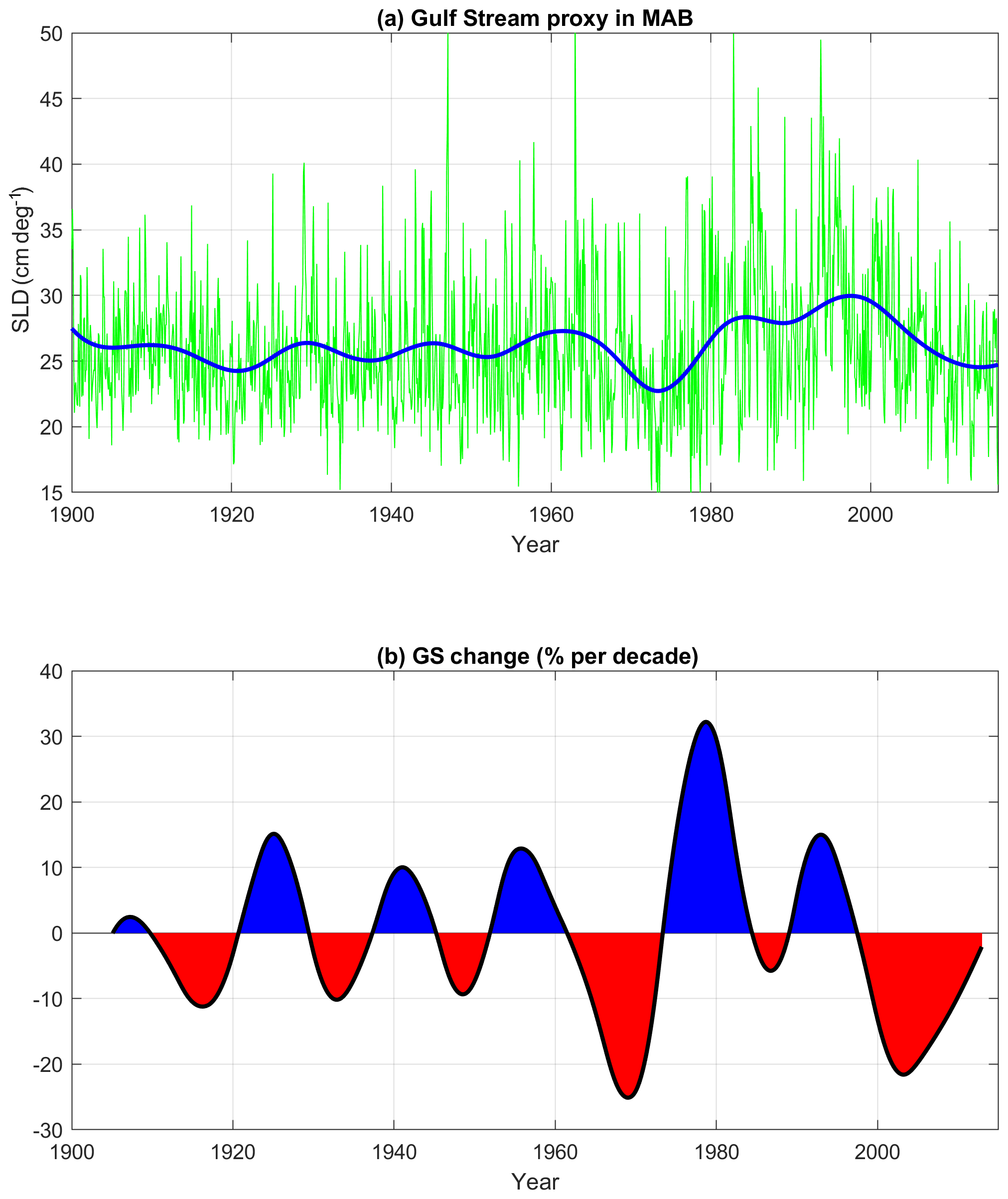
Figure 9 (a) Gulf Stream proxy in the Mid-Atlantic Bight (GS-MAB) calculated from the average change in sea level across the GS; the units are centimeter change per 1^∘ latitude. The green line is for monthly values, and the heavy blue line is the sum of low-frequency EMD modes. (b) The change in the strength of the GS of the low-frequency modes in (a); the units are percentage change per decade, with red and blue representing periods of weakening and strengthening of the GS flow.

Various mechanisms can affect variations in the GS flow such as changes in the strength of the subpolar gyre circulation (Hakkinen and Rhines, 2004) or weakening in the AMOC (Bryden, 2005; McCarthy et al., 2012; Srokosz et al., 2012; Ezer et al., 2013; Smeed et al., 2014, 2018; Blaker et al., 2014; Roberts et al., 2014; Ezer, 2015; Rahmstorf et al., 2015; Caesar et al., 2018). The earlier period of GS weakening in the 1960s–1970s is consistent with observations and models that showed large density changes in the North Atlantic and as much as 30 % weakening in the GS between 1955–1959 and 1970–1974 (Levitus, 1989, 1990; Greatbatch et al., 1991; Ezer et al., 1995). At the time of these early studies, before the age of satellite altimeters, observations were limited and models less sophisticated, so there were some doubts that the large weakening in the GS during the 1960s and 1970s was real. However, this reconstruction by Dangendorf et al. (2019) and another reconstruction of AMOC from sea level data by Ezer (2015) both confirm the results of the early studies, showing only two periods of pronounced weakening in the AMOC since the 1950s. Future observations will show if the recent decline is just a relaxation from the strong GS of the 1980s and 1990s or a continuous downward trend. The relation between the GS-MAB proxy and basin-scale processes is thus analyzed below by looking at two measures: the AMO and AMOC.

3.3.1 The Atlantic Multi-decadal Oscillation (AMO)

The large decadal and multi-decadal variations in the GS-MAB proxy as seen in Fig. 9 are compared with the annual Atlantic Multi-decadal Oscillation index (AMO; Enfield et al., 2001) for 1900–2015 (Fig. 10). EMD is used to compare oscillating modes with similar timescales. High-frequency modes of the GS and AMO are not significantly correlated, but variability in the two time series on timescales of ∼ 10–60 years is correlated, especially the lowest-frequency modes (bottom two panels in Fig. 10), with correlations of 0.5–0.8 that are statistically significant at 95 % (after considering the reduction in degrees of freedom in the low-frequency modes; see explanation in Sect. 2). The wavelet coherence analysis (Appendix A, Fig. A3) principally confirms the sign of these correlations in a 16-year frequency band, though they are not statistically significant. This indicates that the correlations identified by EMD should be taken as preliminary, requiring further data and analyses that are beyond the scope of this paper. Mode 6 (bottom panels in Fig. 10) indicates cyclic behavior at periods up to ∼60 years, consistent with previous studies (Chambers et al., 2012). Various studies indicated a connection between AMO, which represents variations in SST, and sea level. Ezer et al. (2016), for example, showed a change in the sign of the correlation across the GS, which could indicate changes in the GS strength; if sea level rises at one side of the GS and drops at the other side, the change in gradient indicates a change in the strength or position of the GS. The EMD analysis also indicates nonstationary variations with changing amplitude and period over time, showing larger oscillations in all modes after the 1960s, though this might also be related to a decreasing performance in the sea level reconstruction before the 1940s when the tide gauge records become much sparser. It is acknowledged that correlation does not indicate cause and effect and that each EMD mode may not necessarily represent a specific mechanism. For example, for oscillations on timescales of 10–40 years the AMO lags behind the GS by 2–5 years (the second and third panels in Fig. 10), but for longer timescales (bottom panels of Fig. 10) the GS lags behind the AMO by 5–10 years. It is interesting to note that modes 4 and 5 captured the minimum GS-MAB in the 1970s, while mode 6 captured the minimum in the 2000s. The positive correlation between low-frequency variations in the GS and the AMO can be interpreted in several ways – during periods of more intense flow the GS transports more heat to the North Atlantic, thus raising SST and increasing the AMO index (i.e., AMO lags behind the GS). On the other hand, the AMO is connected to slow variations in AMOC that after some delay can impact the GS (i.e., GS lags behind AMO). The low-frequency multi-decadal modes seen here resemble findings from ocean models such as the decadal variations seen in the early Atlantic model of Ezer (1999) and in a realistic Atlantic Ocean model of Sevellec and Federov (2013), who found an oscillatory AMOC mode with a period of ∼24 years and an e-folding decay timescale of ∼40 years that relates to the westward propagation of large-scale temperature anomalies (thus connecting AMOC with the AMO). Therefore, the relation of GS-MAB and the observed AMOC is analyzed next.

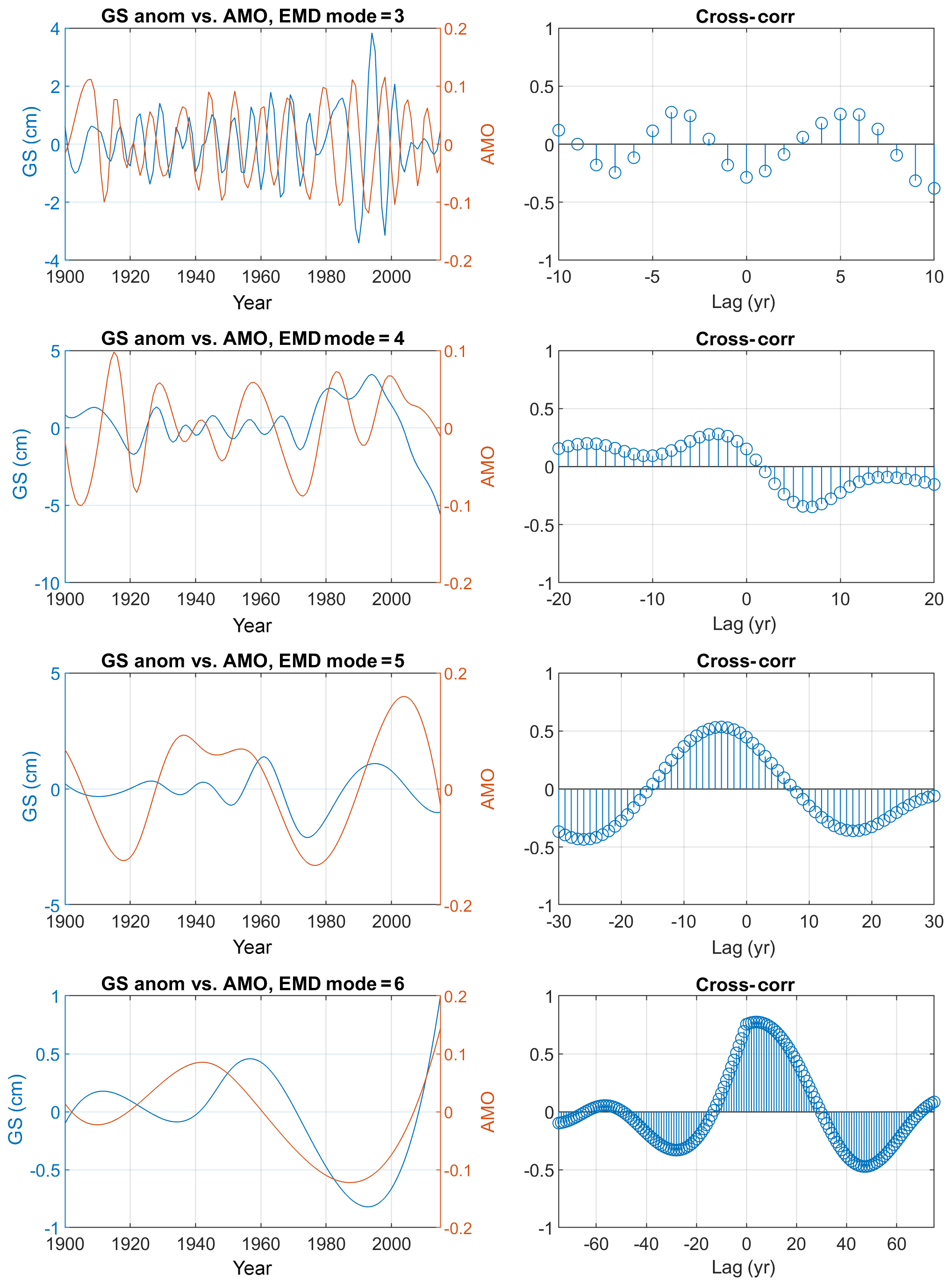
Figure 10 (left) Comparison of EMD oscillating modes of the monthly GS-MAB proxy (blue; units: sea level change across the GS in centimeters per degree latitude) and the AMO index (red). (right) Cross-correlation as a function of lag. There are a total of seven EMD modes; modes 2–6 are the oscillating modes.

3.3.2 The Atlantic Meridional Overturning Circulation (AMOC)

Continuous observations of AMOC transport at 26.5^∘ N are available since 2004 from the RAPID program (McCarthy et al., 2012; Srokosz et al., 2012; Smeed et al., 2014, 2018). Previous studies found connections between AMOC and sea level difference across the GS as derived from two tide gauges (Ezer, 2015), so it is interesting to examine if the reconstructed GS shows a relation to the observed AMOC. The RAPID/AMOC transport is the combined contribution from three sources: the upper mid-ocean (UMO) due to density gradients, wind-driven Ekman (EK) transport and Gulf Stream transport as observed by the cable across the Florida Current (FC). These three components and the total AMOC transport are compared with the proxy GS-MAB record for 2005–2015 (Fig. 11). Shown are the monthly values and the low-frequency EMD modes. The low-frequency variations in the total AMOC transport are significantly correlated (P<0.05) with the GS-MAB proxy (R=0.64), and both show a weakening trend of ∼12 % over this decade of comparison (Fig. 11a). However, the GS-MAB proxy is not significantly influenced by the EK (Fig. 11c; R=0.1) or the FC (Fig. 11d; $R=-\mathrm{0.1}$) components of AMOC. Note that the FC record used by RAPID in Fig. 11d is much shorter than the entire FC record in Fig. 7; thus, the longer record captures lower-frequency modes and shows higher correlation with the GS-MAB (Fig. 7a; R=0.28). It does seem, though, that more than 50 % of the variability in the GS-MAB is due to the UMO (R=0.72). Moreover, the weakening trend in the GS-MAB also seems to be due to the weakening in the UMO (Fig. 11b). The GS-MAB lags behind changes in the UMO by about a year, a result also obtained in Ezer (2015). Coherent oscillations with periods of ∼ 2–3 years dominate the low-frequency modes for GS-MAB, UMO, EK and the total AMOC transport. In summary, it is encouraging that despite the limitation of using only surface and coastal data in the reconstruction, it can capture the variability of AMOC including changes in the subsurface density field (i.e., UMO). It is also noted that in the earlier period of a weakening GS in the 1970s (Fig. 9), changes in the Atlantic density field rather than changes in the wind fields were suggested as the main cause of this weakening (Levitus, 1989, 1990; Greatbatch et al., 1991; Ezer et al., 1995), which is consistent with the finding here of the main cause of the recent period of GS weakening.

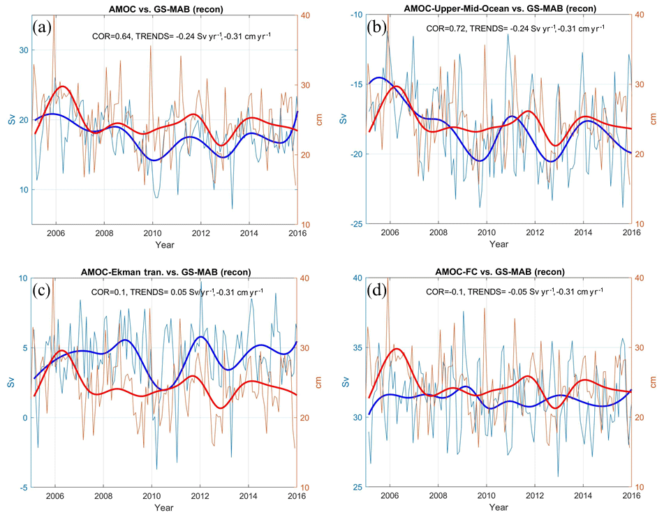
Figure 11 Comparison between the GS-MAB proxy and the RAPID observations: (a) total AMOC transport, (b) upper mid-ocean transport, (c) Ekman transport and (d) the Florida Current transport. The GS proxy (in blue) is the average north–south sea level change across the GS (in centimeters per 1^∘ latitude) representing the eastward-flowing strength of the geostrophic surface flow; RAPID observations (transport in Sverdrups) are in red. Thin lines are monthly values, and the heavy lines represent the sum of low-frequency EMD modes. The correlation of the low-frequency modes and the trends of the monthly records are indicated.

4 Summary and conclusions

Since continuous coverage of global sea level from satellite altimeters started only in recent decades (since the middle 1990s) and century-long tide gauge records are sparse, it is a challenge to study long-term variations in sea level and ocean dynamics (decades to multi-decades and longer) with existing data. Such studies are important for understanding natural variations, anthropogenic changes, and the increased risk to coastal communities from climate change and sea level rise. To overcome the lack of past data and sparse tide gauges data, various statistical optimization techniques were used to reconstruct past global sea level. Here, a new hybrid reconstruction by Dangendorf et al. (2019) for 1900–2015 was examined, with two main goals in sight: first, to evaluate the reconstruction against recent observations in order to see if the global coarse-resolution reconstruction can capture variations in regional coastal sea level and ocean dynamics; and second, to study mechanisms and forcing of long-term variability and their relation to basin-scale modes. The focus of the study was on the southwestern North Atlantic Ocean, where the dynamics are dominated by the variability of the Gulf Stream system and where offshore GS dynamics can drive coastal sea level rise and variability (Blaha, 1984; Leverman et al., 2005; Ezer, 2001, 2013, 2015, 2019; Ezer et al., 2013; Salenger et al., 2012; Yin and Goddard, 2013; Domingues et al., 2018).

Close examination of the western North Atlantic region in the reconstructed sea level shows uneven acceleration in different periods during the 116-year record, with larger acceleration in the last 2 decades than that of previous periods, as indicated globally in Dangendorf et al. (2019) and others. However, regionally, the largest changes in sea level rise rates are found near the GS with often opposing sea level changes north and south of the GS front, thus pointing to the hypothesis that spatial variations in sea level near the GS are linked to changes in the GS strength (and possibly position). To study variations in the GS, a proxy of the GS strength was derived from sea level differences across the GS in two subregions, the SAB and the MAB. Using EMD analysis, long-term (timescales longer than 5 years) variations in the reconstructed GS were found to be significantly correlated with the low-frequency oscillations of the AMO, detecting the two periods of weakening GS. Calculations using wavelet coherence found similar patterns as the EMD calculations, but the correlations were not statistically significant (Appendix A, Fig. A3). Another interesting result is that during the 116-year record, there are two distinct periods of relatively long weakening in the GS flow; each one lasts for at least a decade when the maximum trend was a declining flow of about 20 % per decade to 25 % per decade. The first period with a slowing GS was seen in the 1960s and 1970s. This period of weakening circulation was previously identified by limited observations (Levitus, 1989, 1990) and early basin-scale diagnostic models (Greatbatch et al., 1991; Ezer et al., 1995) that suggested up to 30 % slowdown in the GS transport over a 15-year period (though model results could not be verified due to lack of observations at the time). This weakening was suggested to relate mostly to changes in the subsurface Atlantic Ocean density field and to lesser degree to changes in the wind-driven Ekman transport. Regional acceleration in sea level rise along the US East Coast due to the weakening GS was also seen in models and data during this time (Ezer et al., 1995). However, only years later, based on more data, did the link between weakening in the GS and AMOC and accelerated coastal sea level become a topic of considerable research (e.g., Levermann et al., 2005; Yin and Goddard, 2013; Sallenger et al., 2012; Ezer et al., 2013). The second period of significant weakening in the reconstructed GS was the longest in the 116-year record (∼ 1998–2015; it may continue beyond the reconstruction record). It is noted, though, that the uncertainties of the reconstruction increase substantially before the 1950s, when tide gauge records become sparse. Experiments with 1000 simulations of red noise (Appendix A, Fig. A2) show that obtaining such a long period of GS weakening from random natural variability is extremely rare. During the more recent period significantly more observations exist that support the recent weakening trend, including altimeter data (Ezer et al., 2013; Ezer, 2015; Dong et al., 2019; Zhang et al., 2020), reconstruction from temperature data (Rahmstorf et al., 2015; Caesar et al., 2018) direct measurements of the GS (Rossby et al., 2014; Andres et al., 2020) and the AMOC/RAPID observations (McCarthy et al., 2012; Srokosz et al., 2012; Baringer et al., 2013; Smeed et al., 2014). A comparison of the reconstructed GS and the observed AMOC shows a similar downward trend for 2005–2015 and similar oscillations with periods of 2–5 years. The recent weakening of the reconstructed GS and the variability were correlated with variations in the upper mid-ocean transport component of the AMOC and to lesser degree in recent years by changes in the Ekman transport, somewhat resembling processes suggested in the past to explain the 1960s–1970s changes.

While Dangendorf et al. (2019) validated the RecSL globally, another goal here was to evaluate the reconstructed sea level against recent observations in the study area. Coastal tide gauge data in the lower Chesapeake Bay (in the flood-prone city of Norfolk) for 1927–2015 were compared with the reconstructed sea level offshore (the bay is completely absent from the 1^∘ × 1^∘ coarse-resolution reconstruction). Observations of the Florida Current transport for 1982–2015 were also compared with the reconstructed GS in the SAB. EMD analysis (Huang et al., 1998) was used to decompose the time series into nonstationary modes of different timescales in order to examine what portion of the observed variability can be captured by the reconstruction. The results show that for timescales of ∼5 years and longer, the reconstruction can capture most of the observed variability (correlations of 0.8–0.9) in both the coastal sea level and the FC transport. Wavelet coherence analysis of the FC and GS-SAB (Appendix A) largely confirms the results of the EMD analysis.

In summary, the study demonstrated that despite the coarse horizontal resolution of the global reconstruction (1^∘ × 1^∘) and the sparse data available before the satellite altimetry age, some long-term variations in regional dynamics can be captured quite well by this global reconstruction, therefore providing a useful tool for studies of long-term past variability in other regions as well. The long reconstruction can help studies of decadal and longer natural variability as well as anthropogenic climate change. For example, the study shows that while the ocean circulation and the GS are subject to natural multi-decadal variations, the recent weakening in the GS is unprecedented in length during the 116 years of the reconstruction. It also confirmed the existence of another period of a significantly weakening GS during the 1960s and 1970s, which was previously suggested only by limited observations. Future observations are needed to determine if the recent weakening will last due to anthropogenic forces or recover like the previous slowdown.

Appendix A

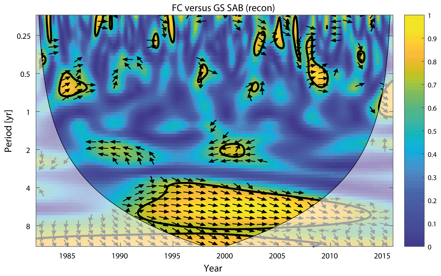
Figure A1 Squared wavelet coherence between the FC transport and GS-SAB time series. The 5 % significance level against red noise is shown as a thick contour. All significant sections above 4 years show in-phase behavior, which is indicated by arrows that are directed to the right.

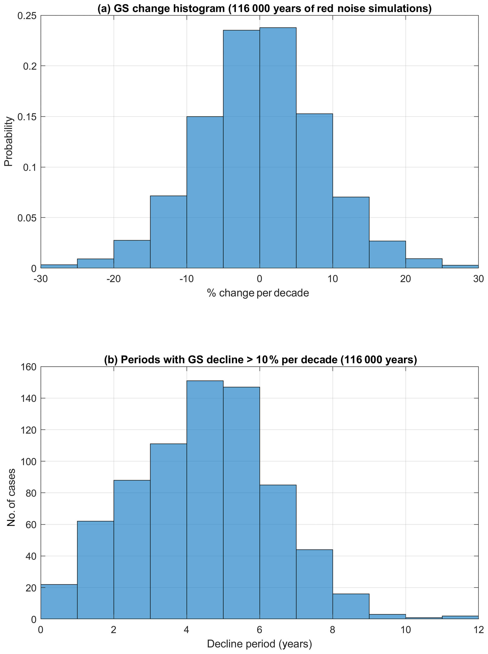
Figure A2 Histogram of the statistics of the GS-MAB flow changes using 1000 realizations of 116 years with random red noise (total of 116 000 years); the simulations imitate the spectrum of the reconstructed GS in Fig. 9a. In each of these simulations GS change was calculated using EMD as in Fig. 9b. (a) The probability of obtaining different GS changes shows that the chance of GS weakening by over 20 % per decade (as seen in the reconstruction) is less than 1 % for any particular month. (b) The distribution of period length with GS flow declining by at least 10 % per decade shows that there were only three cases of GS weakening that last at least 10 years during the 116 000 years. For comparison, the GS-MAB in Fig. 9b shows two such cases in 116 years: a ∼10 year weakening period in the 1970s and a ∼15 year weakening period in the 2000s.

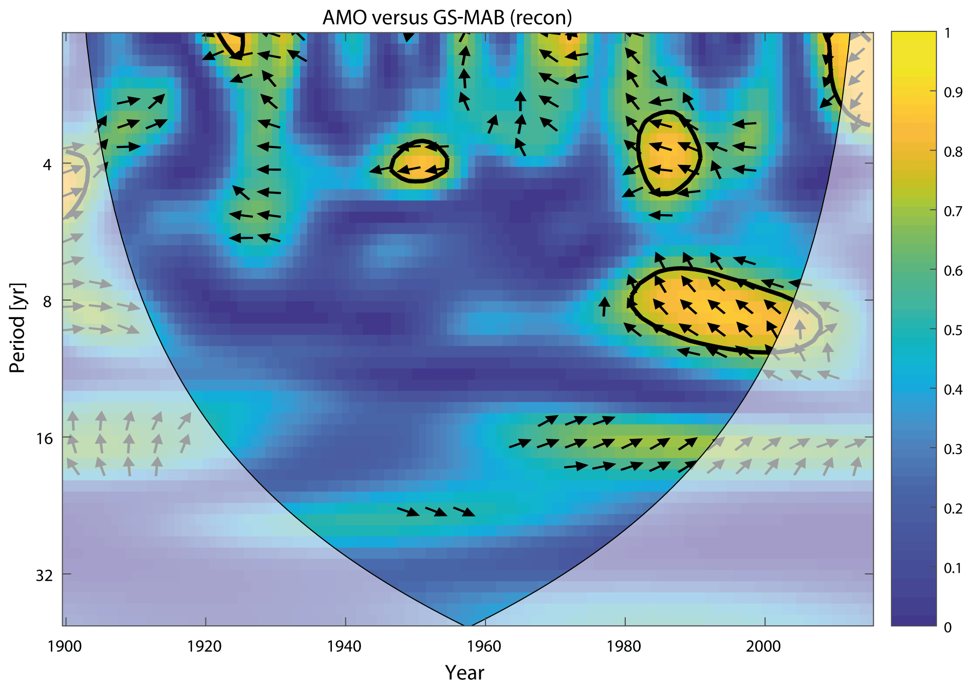
Figure A3 Squared wavelet coherence between the AMO index and GS-MAB time series. The 5 % significance level against red noise is shown as a thick contour. All significant sections (mostly after the 1980s) for periods below 10 years show antiphase behavior, which is indicated by arrows that are directed to the left. Positive, through statistically nonsignificant, correlations are found in the 16-year bands since the 1960s and confirm the low-frequency modes identified by the EMD in the main paper.