The long-term spatiotemporal variability of sea surface temperature in the northwest Pacific and China offshore

The variability of the sea surface temperature (SST) in the northwest Pacific has been studied on seasonal, annual and interannual scales based on the monthly datasets of extended reconstructed sea surface temperature (ERSST) 3b (1854–2017, 164 years) and optimum interpolation sea surface temperature version 2 (OISST V2 (1988–2017, 30 years). The overall trends, spatial–temporal distribution characteristics, regional differences in seasonal trends and seasonal differences of SST in the northwest Pacific have been calculated over the past 164 years based on these datasets. In the past 164 years, the SST in the northwest Pacific has been increasing linearly year by year, with a trend of 0.033 ^∘C/10 years. The SST during the period from 1870 to 1910 is slowly decreasing and staying in the range between 25.2 and 26.0 ^∘C. During the period of 1910–1930, the SST as a whole maintained a low value, which is at the minimum of 164 years. After 1930, SST continued to increase until now. The increasing trend in the past 30 years has reached 0.132 ^∘C/10 years, and the increasing trend in the past 10 years is 0.306 ^∘C/10 years, which is around 10 times that of the past 164 years. The SST in most regions of the northwest Pacific showed a linear increasing trend year by year, and the increasing trend in the offshore region was stronger than that in the ocean and deep-sea region. The change in trend of the SST in the northwest Pacific shows a large seasonal difference, and the increasing trend in autumn and winter is larger than that in spring and summer. There are some correlations between the SST and some climate indices and atmospheric parameters; the correlations between the SST and some atmospheric parameters have been discussed, such as those of the North Atlantic Oscillation (NAO), Pacific Decadal Oscillation (PDO), Southern Oscillation Index (SOI) anomaly, total column water (TCW), NINO3.4 index, sea level pressure (SLP), precipitation, temperature at 2 m (T2) and wind speed. The lowest SST in China offshore basically occurred in February and the highest in August. The SST fluctuation in the Bohai Sea and Yellow Sea (BYS) is the largest, with a range from 5 to 22 ^∘C; the SST in the East China Sea (ECS) is from 18 to 27 ^∘C; the smallest fluctuations occur in the South China Sea (SCS), maintained at range of 26 to 29 ^∘C. There are large differences between the mean and standard deviation in different sea regions.

1 Introduction

The ocean is one of the important components of the ocean–atmosphere coupling system (Chelton and Xie, 2010; Wu et al., 2019a, b, 2020). Relative to the atmosphere, the ocean has characteristics such as slow change and large heat capacity (England et al., 2014). Because of the gradual changes in the ocean, climate change at the interannual, decadal and longer timescales may be closely related to the ocean (Trenberth and Hurrell, 1994; Ault et al., 2009). Sea surface temperature (SST) is the basis for the interaction between the ocean and the atmosphere (Wu et al., 2019c, d), and it characterizes the combined results of ocean heat content (Buckley et al., 2014; Griffies et al., 2015) and dynamic processes (Takakura et al., 2018). It is a very important parameter for climate change and ocean dynamics processes, and reflects sea–air heat and water vapor exchange. Observations and numerical simulations show that large-scale sea surface temperature anomalies of over 20^∘ in longitude and latitude can cause significant changes in atmospheric circulation, such as the El Niño and La Niña phenomena (Chen et al., 2016; Zheng et al., 2016). During El Niño, the trade winds in the tropical eastern Pacific are weakened, and the SST increased significantly, which was 3–5 ^∘C higher than normal years. As a result, major changes have been made in the atmospheric circulation and ocean circulation, which have caused the worldwide atmospheric and marine environment and the abnormality of climate (Li et al., 2017).

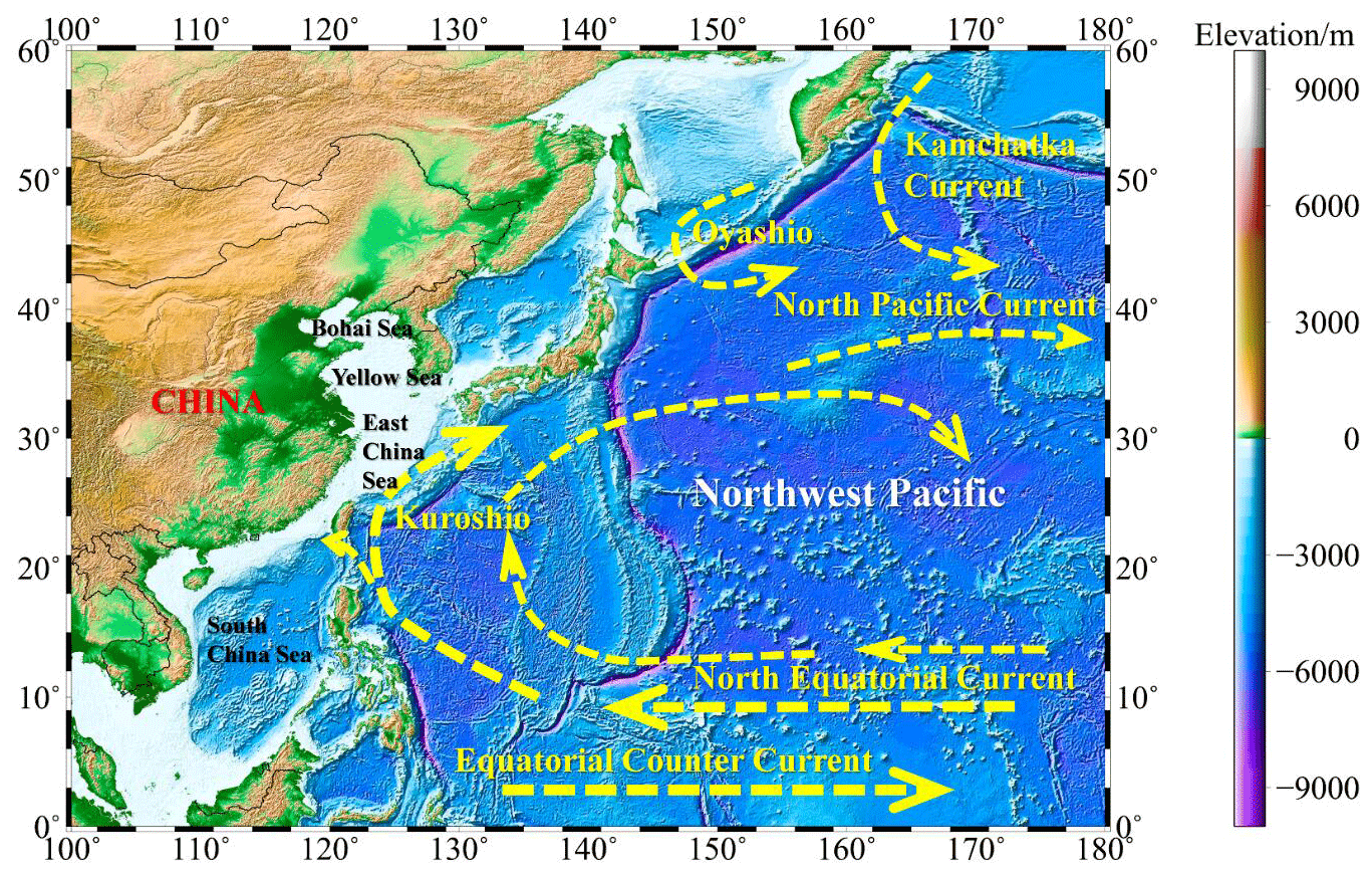
Figure 1 Bathymetric map of the northwest Pacific and ocean circulation.

The northwest Pacific is particularly affected by the El Niño in the eastern Pacific and determines the oceanic climate change in China (Hu et al., 2018). On one hand, climate change causes an increasing SST in the northwestern Pacific, which increases the vertical stratification of the water, affects the atmospheric circulation and changes the intensity and period of coastal winds and upwelling. On the other hand, the 10-year periods of the Pacific Decadal Oscillation (PDO) and the El Niño–Southern Oscillation (ENSO) occur on average every 2 to 7 years, resulting in large variations in upwelling (Xiao et al., 2015; Yang et al., 2017; Xue et al., 2018). These factors will all lead to the impact on the marine environment in Chinese coastal areas, causing land-based droughts, floods and climate disasters (Xu et al., 2018). Therefore, it is very urgent to study the impact of climate change on SST in the northwest Pacific and China offshore. As one of the main parameters of global climate change and one of the important characterizations and predictors of El Niño, the study of SST changes is particularly important.

Previous scholars have done a lot of work on the changing trend of SST. According to the Fifth Assessment Report (AR5) of the Intergovernmental Panel on Climate Change (IPCC), the global SST warming trend was 0.064 ^∘C/10 years between 1880 and 2012 (Pachauri et al., 2014). In fact, many studies have shown that the Pacific SST anomalous changes are closely related to global and regional climate changes, and they have multi-scale temporal variations (Graham, 1994; Latif, 2006; Shakun and Shaman, 2009; Li et al., 2014). In addition, ENSO and PDO, which are closely linked to global and regional climate change, are found in this area. Therefore, the Pacific is one of the key ocean areas that scholars have studied for a long time (Bao and Ren, 2014; Mei et al., 2015; Stuecker et al., 2015; Wills et al., 2018).

So far, two types of main meteorological SST datasets have been obtained: one based on measured mid-resolution (1–5^∘) 100-year datasets and the other based on satellite high-resolution (1–10 km) decadal datasets (Wang et al., 2011; Smith et al., 2014; Huang et al., 2015, 2016; Diamond et al., 2015). The former has rebuilt a time series of months over 150 years and the latter has accumulated over 30 years of time series on a daily average basis (Tian et al., 2019). The existing climatic datasets already have conditions for allowing the creation of a natural mode of change in SST in terms of duration and resolution (Liu et al., 2017; Wang et al., 2018). With the continuous improvement of ocean observation technology and the accumulation of satellite remote sensing data, the conditions for the scholars to use the satellite data for short-term climate change research have been met. In recent years, the research and discussion on the interannual change of SST based on satellite remote sensing SST has attracted wide attention (Tang et al., 2003; Yang et al., 2013; Zhang et al., 2015; Skirving et al., 2018).

Satellite remote sensing can achieve large-area simultaneous measurements with high temporal and spatial resolution. The remote sensing SST obtained is conducive to a more comprehensive and rapid understanding of oceanographic phenomena that affect the ocean surface, including El Niño (Robinson, 2016). At present, about 30 years of satellite remote sensing SST data have been accumulated (Franch et al., 2017), and a set of sea surface temperature data has been provided to study the conditions for the occurrence and development of ocean surface heat change modes in the temporal and spatial span and resolution. So, satellite remote sensing SST has received widespread attention in recent years.

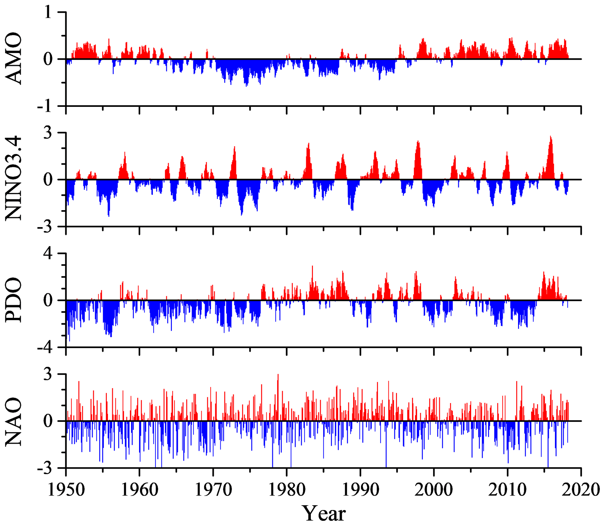
Figure 2 Atlantic Multidecadal Oscillation (AMO) index (a), NINO3.4 index (b), PDO index (c) and NAO index (d) during 1950–2017.

At present, based on satellite remote sensing data, the timescales for the study of changes in SST in the northwest Pacific, especially in China offshore, are mostly within 20 years, which is relatively short for studying climate change (Song et al., 2018; Pan et al., 2018). Most of the research is targeted at specific local sea areas, and there is less research on the changes of the SST in the northwest Pacific covering all marginal seas of China. Therefore, it is necessary to study the SST variation of large-scale and long-term sequences based on satellite remote sensing data.

Previous scholars have made great contributions to the study of global warming, but most of them are the overall changes in the regional average SST, and they tend to ignore the characteristics of changes in certain key sea areas. There are great differences in the trends of SST in different sea areas. The long-term trends of the SST changes in the northwest Pacific (0–60^∘ N, 100–180^∘ E) over the past 164 years (1854–2017) have been calculated based on the monthly datasets of extended reconstructed sea surface temperature (ERSST) 3b in this study. The temporal and spatial distribution characteristics of SST, the overall long-term trend, the regional variation of the seasonal trend and the seasonal differences were analyzed. The correlations with SST changes and climate parameters and indices have been analyzed. To provide a reference for the study of global climate change, the characteristics of SST changes in China offshore have been studied in this paper.

High-spatial-resolution SST datasets including average SST field and monthly SST anomaly (SSTA) field have been obtained. In view of the fact that there are many interannual and intra-annual changes, this paper analyzes the characteristics of SST changes based on these datasets. The trend, the interdecadal changes in SST and their causes, and the correlations with the climate parameters and indices such as NINO3.4 index are relatively low. The ocean thermal dynamic phenomenon is preliminarily discussed. The datasets are processed and analyzed to study the trend changes of SST in the northwest Pacific, to explore the correlation and response mechanisms with climate systems such as ENSO and PDO, and to conduct a detailed analysis of typical sea areas.

2 Study region, data and methods

2.1 Study region

The northwest Pacific is the northwest region of the Pacific, defined as the offshore region of 0–60^∘ N and 100–180^∘ E in this study (Fig. 1). There are more tropical cyclones over the northwest Pacific than any other sea area in the world, with an average annual average of 35. About 80 % of these tropical cyclones will develop into typhoons. On average, about 26 tropical cyclones per year reach at least the intensity of tropical storms, accounting for about 31 % of the global tropical storms, and are more than double the number of any other area. The sea–air interaction in this area is very strong and the change of SST is worth exploring.

Figure 3 The temporal variability of annual SST.

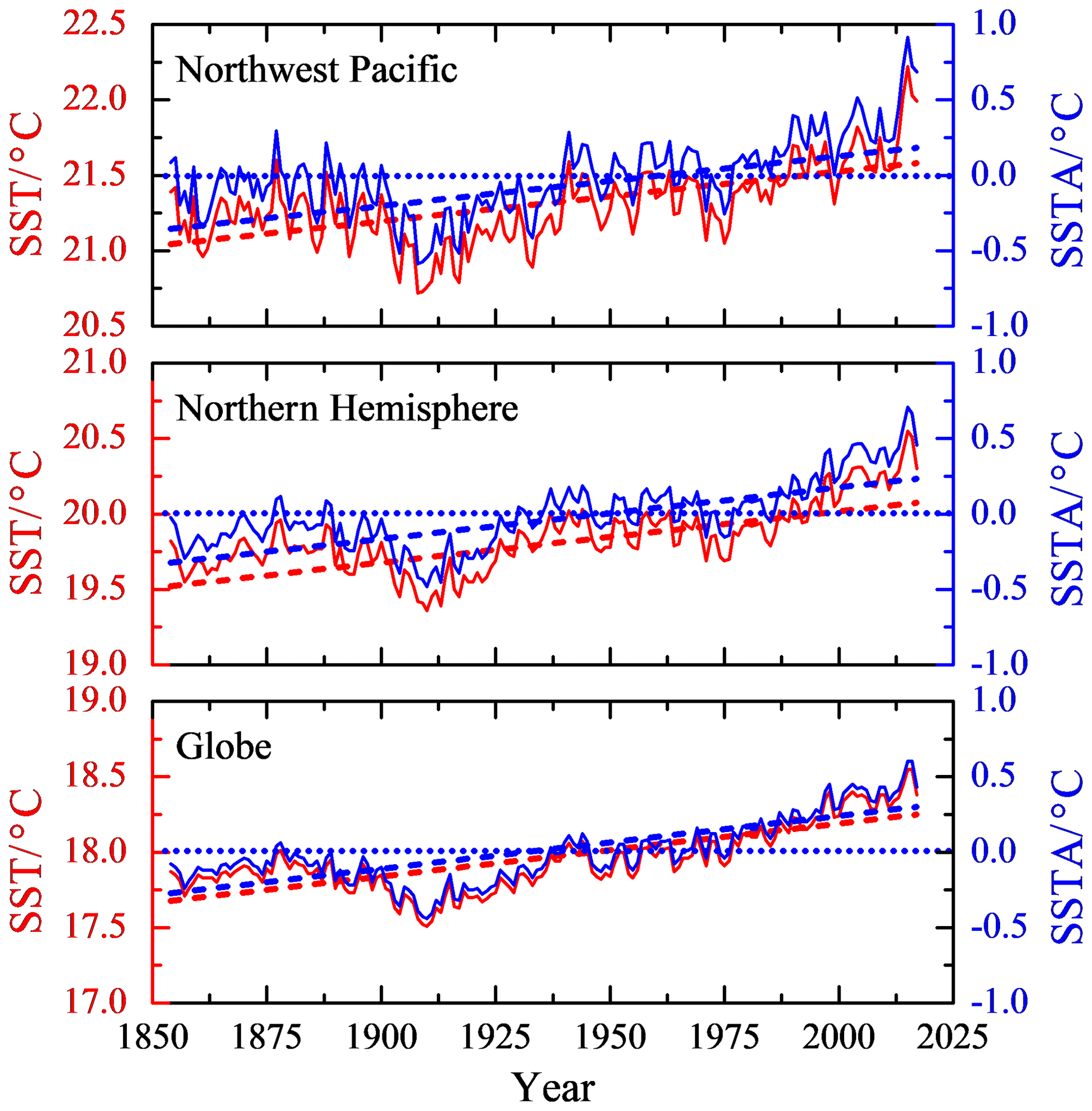
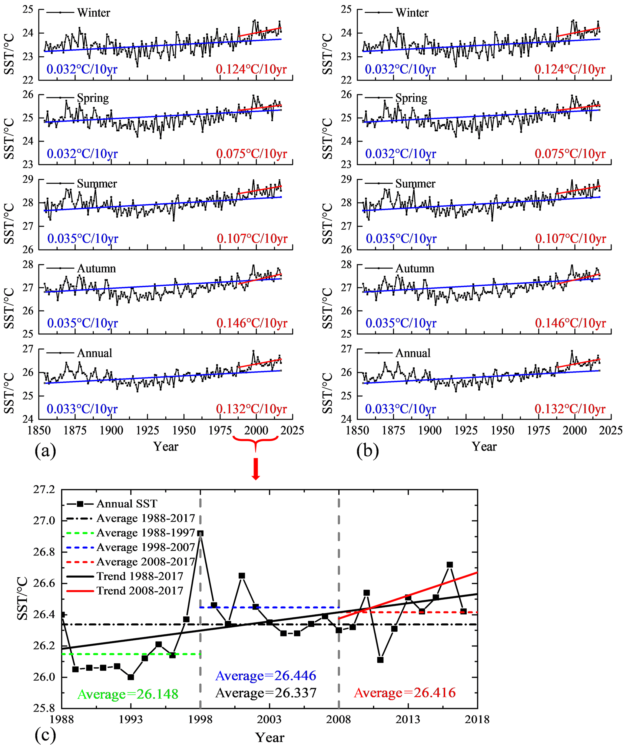
Figure 4 Variability of seasonal/annual SST. (a) The annual SST over the 1854–2017 period; (b) the SST anomaly over the 1854–2017 period; (c) the SST over the 1988–2017 period (the last 30 years).

2.2 SST dataset

Several data sources are used to analyze the long-term temporal and spatial variability of SST in the northwest Pacific in this present study. Long-term statistics are based on the monthly SST data from ERSST 3b (1854–2017) (Smith et al., 2008). The ERSST dataset is a global monthly sea surface temperature analysis derived from the International Comprehensive Ocean–Atmosphere Dataset with missing data filled in by statistical methods. This monthly analysis begins in January 1854 and continues to the present (https://www1.ncdc.noaa.gov/pub/data/cmb/ersst/v3b/, last access: 3 January 2020). The primary SST dataset analyzed in this study is the NOAA optimum interpolation sea surface temperature V2 (OISST V2 1982–2017; http://www.esrl.noaa.gov/psd/data/gridded/data.noaa.oisst.v2.html, last access: 29 December 2019) (Reynolds et al., 2002, 2007). There are many SST datasets, such as the Hadley Centre Sea Ice and Sea Surface Temperature (HadISST1) dataset, which replaces the Global sea-Ice and Sea Surface Temperature (GISST) datasets and is a unique combination of monthly globally complete fields of SST and sea ice concentration on a 1^∘ latitude–longitude grid from 1870 to date. However, from May 2007, the dataset of in situ measurements used in the HadISST dataset has changed. The advantage of this dataset is apparent when compared with other gridded datasets such as HadISST, ERSST and OSTIA, which spans only the period starting from 2007.

The seasonal mean data are obtained by averaging the monthly average SST after the above-mentioned processing. The spring is March, April and May (MAM), the summer is June, July and August (JJA), the autumn is September, October and November (SON), and the winter is December of the previous year and January and February (DJF).

The SST anomaly is the deviation from the long-term SST average of the observations of the SST describing a particular area and time. The year anomaly represents the deviation of the average of the SST for a given year from the mean of the multi-year SST. The month anomaly represents the deviation of the average of the SST for a particular month from the average of the SST for that particular month for many years. In this paper, the mean value from 1854 to 2017 is taken as the climate mean state, and the sea surface temperature anomaly is subtracted from the SST field to obtain the SSTA field.

Table 1 The average trend of SST (unit: ^∘C/10 years).

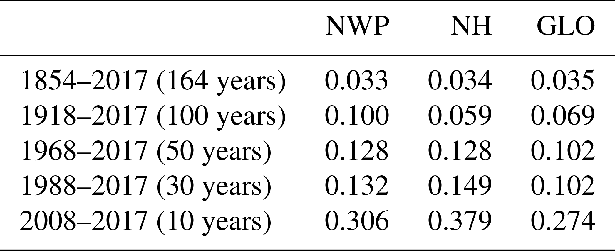
NWP: northwest Pacific; NH: Northern Hemisphere; GLO: globe. All the trends are significant at the 95 % confidence level.

2.3 Climate index dataset

The Atlantic Multidecadal Oscillation (AMO) is a climate cycle that affects the SST of the North Atlantic Ocean based on different modes on multidecadal timescales (http://www.esrl.noaa.gov/psd/data/timeseries/AMO, last access: 1 December 2019; McCarthy et al., 2015). NINO3.4 index uses SST to characterize ENSO; the NINO3.4 SST region consists of temperature measurements between 5^∘ N and 5^∘ S and 120–170^∘ W (Gergis and Fowler, 2005). The PDO index is the time coefficient of the first mode obtained by performing the empirical orthogonal function (EOF) of the mean SSTA to the north of 20^∘ N in the North Pacific (http://jisao.washington.edu/pdo/PDO.latest, last access: 30 September 2018). The North Atlantic Oscillation (NAO) is the most prominent modality in the North Atlantic. Its climate impact is most prominent mainly in North America and Europe, but it may also have an impact on the climate in other regions such as Asia. Recent studies have not only further confirmed its existence but also revealed its connection with a wide range of oceans and atmospheric conditions.

The correlation between the SST and the atmospheric parameters is analyzed based on the ERA-Interim data. ERA-Interim refers to the European Centre for Medium-Range Weather Forecasts (ECMWF), which is an independent intergovernmental organization supported by 34 countries. Its goal is to develop numerical methods for midterm weather forecasting. The country provides forecasting services, conducts scientific and technological research to accumulate forecasts, and accumulates meteorological data. ERA-Interim is the latest global reanalysis product developed by ECMWF. The weather data and climate data from January 1988 to December 2017 are used in this paper, such as sea surface temperature, sea-to-air interface heat flux and wind field data at a height of 10 m; the spatial resolution of these datasets is $\mathrm{1.5}{}^{\circ }\times \mathrm{1.5}{}^{\circ }$.

2.4 Methods

Regression analysis is an important part of mathematical statistics and multivariate statistics. It is a mathematical method to study the correlation between variables and variables. The regression analysis has a wide range of applications in the statistical forecasting of oceans and atmospheres. It is used to analyze the statistical relationship between a variable (called forecast) and one or more independent variables (called predictions) and to establish a forecast. The regression equation is produced by the quantity and forecast factor, and then based on this equation to make predictions of the forecast volume. Regression analysis includes linear regression and non-linear regression. The linear regression is commonly used, and a linear regression analysis method is used in this paper.

Use x_i to represent a climate variable with a sample size of n. Use t_i to represent the time corresponding to x_i and establish a linear regression between x_i and t_i. The formula can be expressed as

$$\begin{array}{}\text{(1)}& x_i=a+b{t}_i,i=\mathrm{1},\mathrm{2},\mathrm{3},\mathrm{\dots },n,\end{array}$$

where a is the regression constant and b is the regression coefficient. a and b can be calculated using the least-squares method.

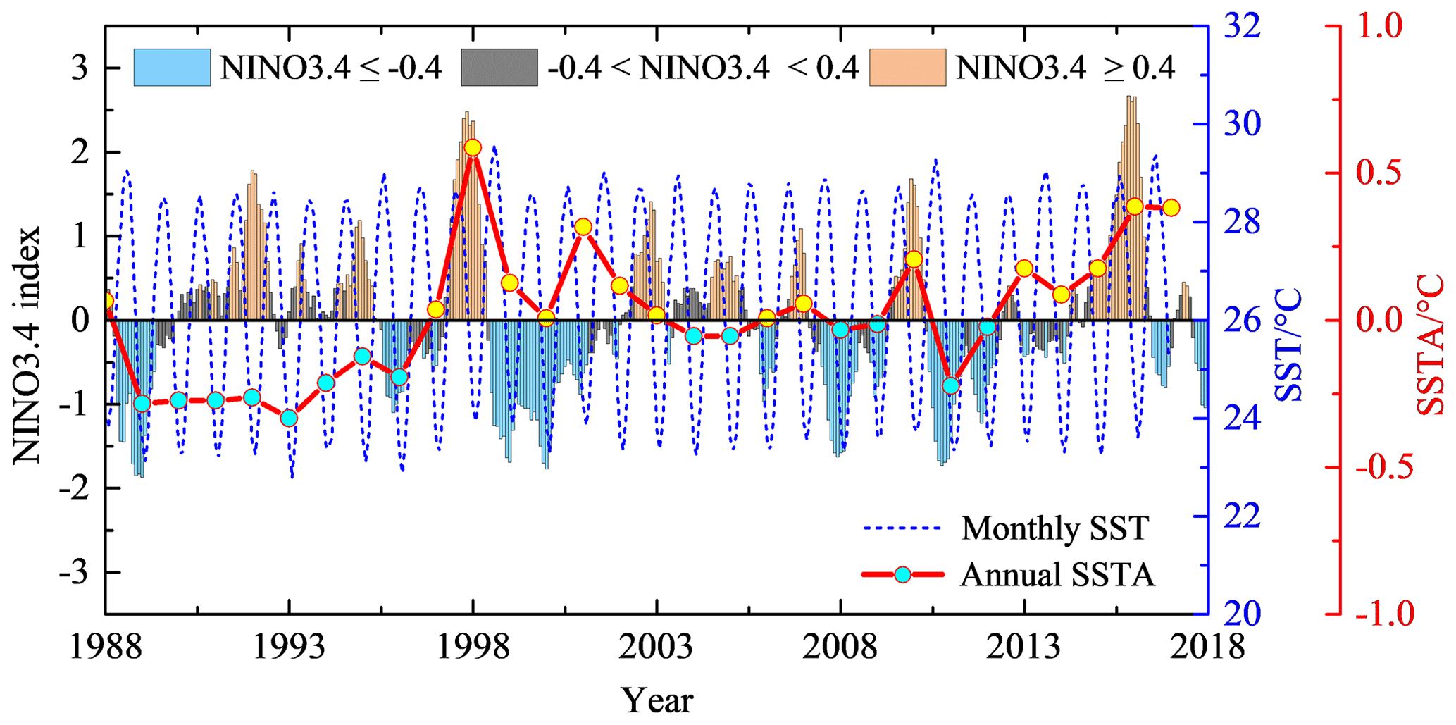
Figure 5 The NINO3.4 index and SST/SSTA during 1988 to 2017. (El Niño is in pink and La Niña is in blue.)

For the observation data x_i and the corresponding time t_i, the least-squares calculation result of the regression coefficient b and the constant a is expressed as

$$\begin{array}{rl}& b={\displaystyle \frac{\sum _{i=\mathrm{1}}^n\left(x_i-\stackrel{\mathrm{‾}}{x}\right)\left(t_i-\stackrel{\mathrm{‾}}{t}\right)}{\sum _{i=\mathrm{1}}^n{\left(x_i-\stackrel{\mathrm{‾}}{x}\right)}^{\mathrm{2}}}}\\ & a=\stackrel{\mathrm{‾}}{x}-b\stackrel{\mathrm{‾}}{t}.\end{array}$$

The correlation coefficient between time t_i and x_i is

$$\begin{array}{}\text{(2)}& r=\sqrt{{\displaystyle \frac{\sum _{i=\mathrm{1}}^n{t}_i^{\mathrm{2}}-\frac{\mathrm{1}}{n}{\left(\sum _{i=\mathrm{1}}^n{t}_i\right)}^{\mathrm{2}}}{\sum _{i=\mathrm{1}}^n{x}_i^{\mathrm{2}}-\frac{\mathrm{1}}{n}{\left(\sum _{i=\mathrm{1}}^n{x}_i\right)}^{\mathrm{2}}}}}.\end{array}$$

The correlation coefficient r is expressed as the degree of closeness of the linear correlation between the variable x and the time t. When r > 0, b > 0, indicating that x increases with time t; when r < 0, b < 0, indicating that the variable x decreases with time t. A significance test is performed on the correlation coefficient to determine the significance level α (confidence is 1α) first. If |r|>r_α, this shows that the trend of the variable x with time t is significant; otherwise, it is not significant.

Figure 6 Spatial distribution of monthly SST over the 1988–2017 period.

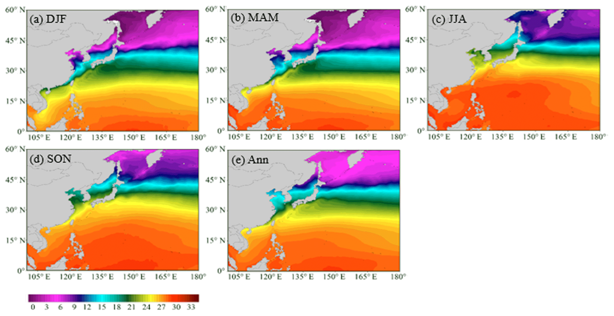
Figure 7 Spatial distribution of seasonal/annual SST over the 1988–2017 period: (a) winter: DJF; (b) spring: MAM; (c) summer: JJA; (d) autumn: SON; (e) annual.

3 Results and discussion

3.1 Temporal distribution of SST

With the gradual warming of the global climate, the average temperature of the ocean is also rising. In order to reflect the overall trend of SST in the northwest Pacific over the past 164 years (1854–2017), the average monthly SST data from 1854 to 2017 were used. The time series curve of SST in the northwest Pacific, the Northern Hemisphere and the global ocean was obtained by processing, and the overall trend of the SST was analyzed, as shown in Fig. 3. As can be seen from the figure, SSTs in the different regions have shown an increasing trend and SST has shown a significant increasing trend since the 20th century.

The SST datasets were used to calculate the SST anomaly time series and its linear variation trend in the northwest Pacific, the Northern Hemisphere and the global ocean, as shown in Fig. 3. The slope of the linear equation with one unknown obtained by least-squares fitting is the annual change rate of SST, as shown in Table 1. It shows the increasing trend of SST at different timescales. It can be seen that the data show that the SST in the different regions has shown a significant warming trend as a whole. It can be seen from Table 1 that, from 1854 to 2017, the SST trend of northwest Pacific, Northern Hemisphere and global ocean has increased by 0.033 to 0.035 ^∘C per 10 years. In the past 50 years, the increasing rate of SST has reached 0.10 ^∘C/10 years or more, and the increasing rate in the last 10 years has reached 0.30 ^∘C. It can be seen that the warming trend of SST in the northwest Pacific is very significant.

There exist decadal to multidecadal variations in the SST and SST anomalies series, with a general cool period from the 1880s to the 1910s, a weak warm period from the 1920s to the 1940s, a weak cool period from the 1970s to the 1980s and a recent warm period from the 1990s to the present. Figure 3 also shows that the interannual to decadal variability is larger in the northwestern Pacific, and it is smaller in the global ocean, indicating an increase in SST anomaly variability with the area. It is also interesting to note that the last 10 years see a larger increasing trend of annual mean SST than that for the last 164, 100, 50 and 30 years, indicating an obvious speed-up of warming of the northwest Pacific, Northern Hemisphere and global ocean occurs in the last 10 years, and the growth rate over the past decade has been around 10 times that of the past 164 years.

In the past 164 years, the correlation coefficient of SST trends in the northwest Pacific was 0.73. It passed the 95 % significance test, which shows that the linear trend is significant, and the regression coefficient is 0.0033. This shows that, in the past 164 years, the SST in the northwest Pacific has been increasing linearly year by year at a rate of 0.033 ^∘C/10 years. It can be seen from Fig. 3 that during the period of 1870–1910, the SST slowly decreased, staying in the range between 25.2 and 26.0 ^∘C; during the period of 1910–1930, the SST as a whole maintained a low value, and the change range was small, which is at the minimum over 164 years; since 1930, the SST has started to rise and the trend has continued to this day.

In order to demonstrate the seasonal variation of the SST trend in the northwest Pacific, the SST at $\mathrm{1}{}^{\circ }\times \mathrm{1}{}^{\circ }$ at each grid point in the northwest Pacific was averaged from 1854 to 2017 by winter, spring, summer, autumn and year in this study. The season-by-season linear trend of SST at each grid point has been analyzed. At the same time, the season-by-season time series of the SST anomalies were calculated and the seasonal variation of the comparison trends was shown in Fig. 4.

Figure 4a and b show seasonal and annual mean SST and SST anomalies series. The blue lines are their trends of every seasonal mean SST and SST anomaly series for the western Pacific during 1854–2017; the red lines are their trends during 1988–2017. The increasing trends during 1854–2017 are between 0.032 and 0.035^∘/10 years for all seasons. The seasonal pattern for the last 30 years shows a more significant warming trend than that over the 164-year period. Significant warming occurs in all seasons, with those of autumn and winter being the largest, reaching 0.146 and 0.124^∘/10 years, respectively, during the last 30 years, and that of spring the smallest.

An El Niño or La Niña event is identified if the NINO3.4 index exceeds +0.4 ^∘C for El Niño or −0.4 ^∘C for La Niña, so ±0.4 ^∘C is used for discriminating anomalies in this study. The magenta points indicate that the SST anomaly is larger than 0.4 ^∘C, and the cyan points indicate that the SST anomaly is smaller than −0.4 ^∘C in Fig. 4b. As can be seen from the figure, during the period from 1890 to 1960, there were more negative anomalies and less than −0.4 ^∘C, indicating that there was a cool period during this period. In the period from 1988 to 2017, there are more positive anomalies and more than 0.4 ^∘C, indicating that there was a warm period in the past 30 years.

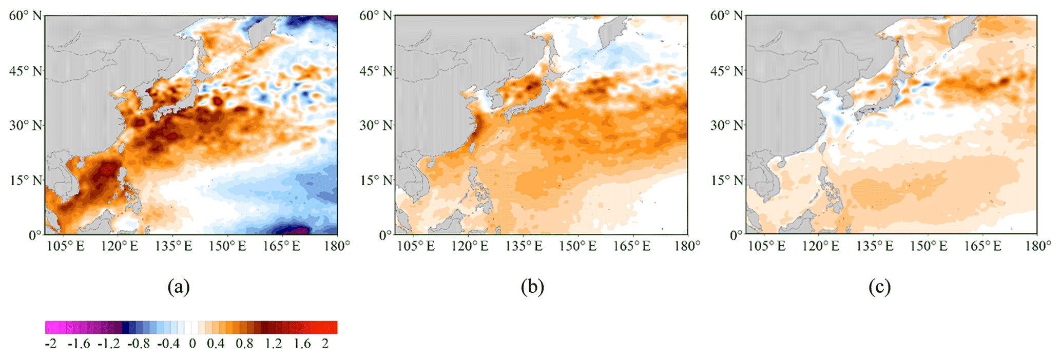
Figure 8 (a) Annual 1998 minus 1988–2017; (b) annual 1998–2007 minus 1988–1997; (c) annual 2008–2017 minus 1988–2017.

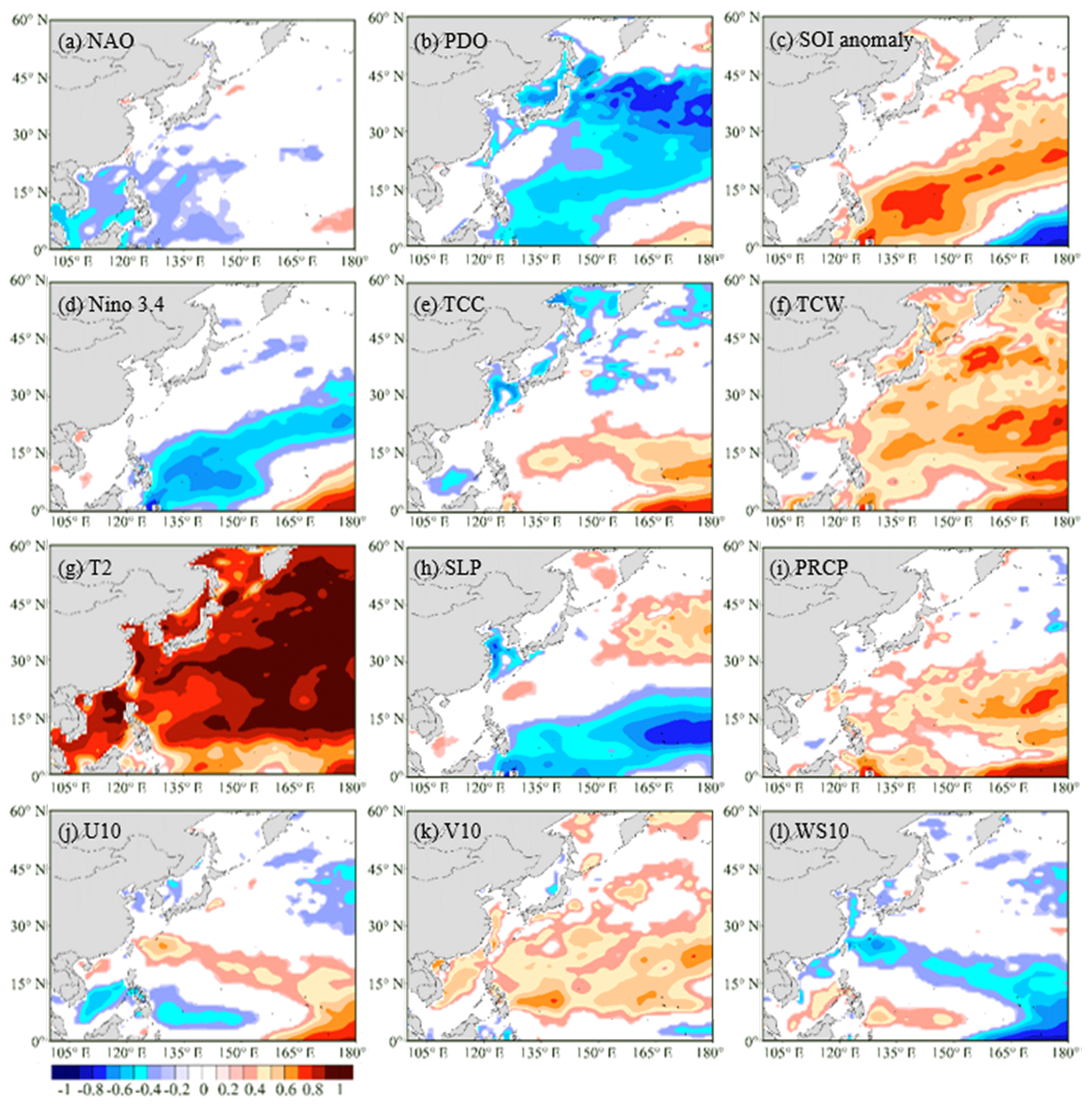
Figure 9 The correlation coefficient between SST and the atmospheric components (level of significance equal to 0.05).

In the analysis of the SST changes in the northwest Pacific during the past 164 years, it has been found that there was a strong warming trend in SST over the past 30 years since 1988. It had been shown that the SST in the northwest Pacific had an overall warming trend starting from the 1970s in the previous studies (Zhou et al., 2009; Kosaka and Xie, 2013) and this study. The time series of the SST in the northwest Pacific from 1988 to 2017 was plotted as shown in Fig. 4c.

Yamamoto's (1986) method has been used to determine the extremum point, and the formula is

$$\begin{array}{}\text{(3)}& R_{\mathrm{SN}}={\displaystyle \frac{\left|\stackrel{\mathrm{‾}}{X_{\mathrm{1}}}-\stackrel{\mathrm{‾}}{X_{\mathrm{2}}}\right|}{S_{\mathrm{1}}+S_{\mathrm{2}}}},\end{array}$$

where $\stackrel{\mathrm{‾}}{X_{\mathrm{1}}}$, $\stackrel{\mathrm{‾}}{X_{\mathrm{2}}}$, S₁ and S₂ are the average and standard deviation of the two stages before and after the extreme year. It was found that there were six stations when $X_{\mathrm{1}}=X_{\mathrm{2}}=\mathrm{10}$, R_SN≥0.7 in 10 years before and after 1998/1999, and the significance level of the statistic reached α=0.05, according to which the SST was considered to have a extremum in this year. The difference between the mean value of the anomaly before and after the extreme was 0.30 ^∘C, and similar results can also be seen in Fig. 4c. It can be found that, in the past 30 years, the SST in the northwest Pacific has significantly warmed up as a whole. The highest annual mean SST appears in 1998, and the temperature has undergone a weak decreasing trend since then, but the average SST during 1998–2007 reaches 26.446 ^∘C, which is higher than around 0.3 ^∘C during 1988–1997. In the last 30 years of SST in the northwest Pacific, the increasing trend in the last 10 years has been obviously greater than the trend in the last 30 years.

The monthly average sea surface temperature in the northwest Pacific is represented by an undulating curve, as shown by the dashed blue line in Fig. 5, and the sea surface temperature anomaly is a dotted red line. The positive value is filled in yellow, and the negative value is filled in cyan. The NINO3.4 index is one of several ENSO indicators based on sea surface temperatures. NINO3.4 is the average sea surface temperature anomaly in the region bounded by 5^∘ N to 5^∘ S, from 170 to 120^∘ W. This region has large variability on El Niño timescales and is close to the region where changes in local sea surface temperature are important for shifting the large region of rainfall typically located in the far western Pacific. An El Niño or La Niña event is identified if the 5-month running average of the NINO3.4 index exceeds +0.4 ^∘C for El Niño or −0.4 ^∘C for La Niña for at least 6 consecutive months.

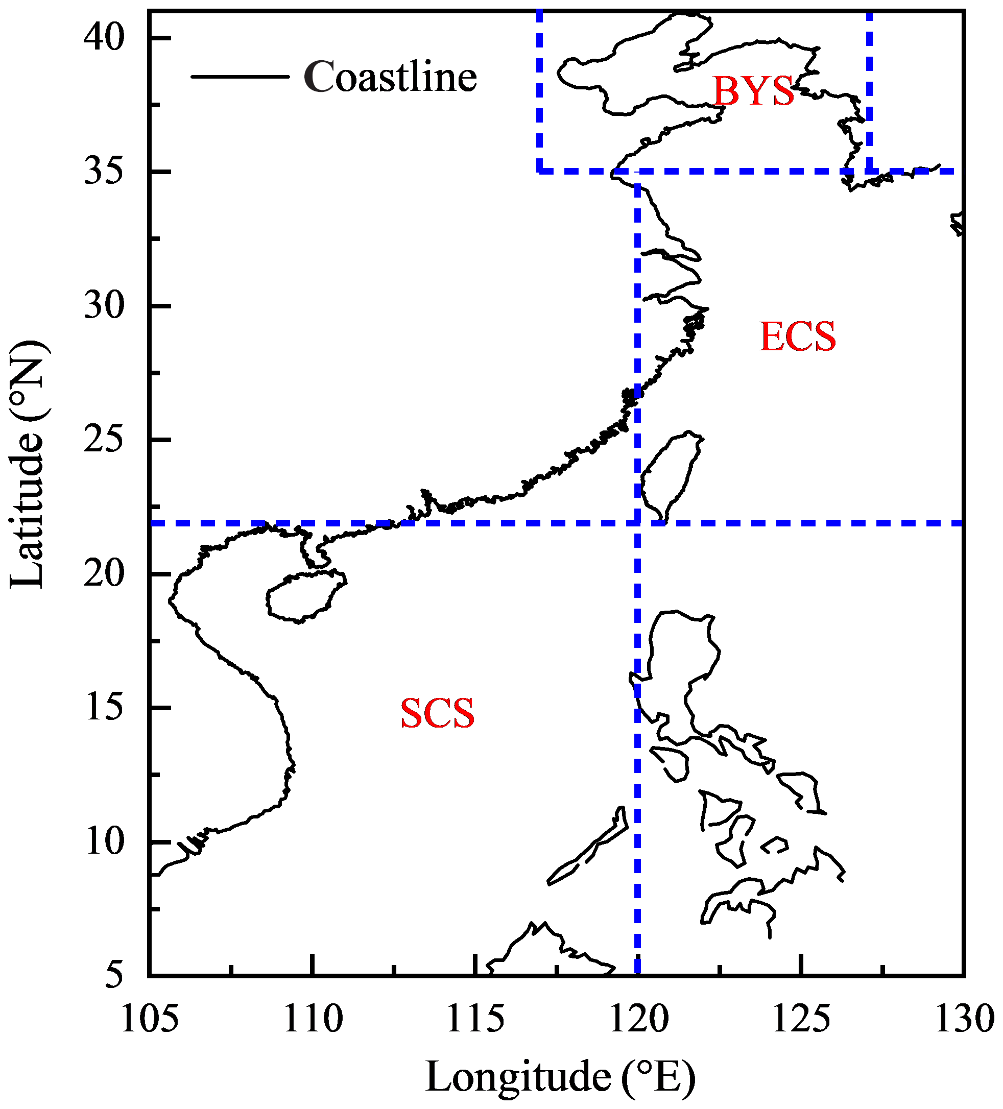
Figure 10 Study regions defined in this paper.

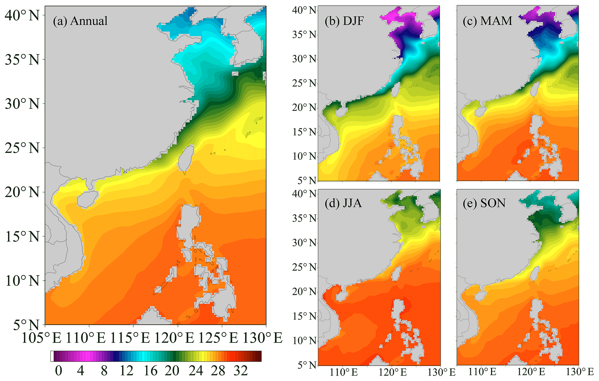
Figure 11 Annual (a) and seasonal (b, c, d, e) mean SST distribution during 1988–2017 in the China Sea: (a) annual; (b) winter: DJF; (c) spring: MAM; (d) summer: JJA; (e) autumn: SON.

It can be seen from Fig. 5 that the SSTA minimum value point occurs from 1989 to 1996; the maximum value point occurs in 1998 and 2016, and the maximum year coincides with the El Niño year. It is shown that the anomalous changes of the SST in the northwest Pacific are closely related to the occurrence year of ENSO. The changes of the SST in the northwest Pacific are obviously affected by the anomalous changes of SST in the equatorial Pacific. The average SSTA was basically negative before 1996 and the basic value after it was positive. That is, the average SSTA was generally lower than the average of 1988–2017 before 1996, and the average SSTA after 1996 was basically higher than the average of 1988–2017, which is also reflected in Fig. 4c.

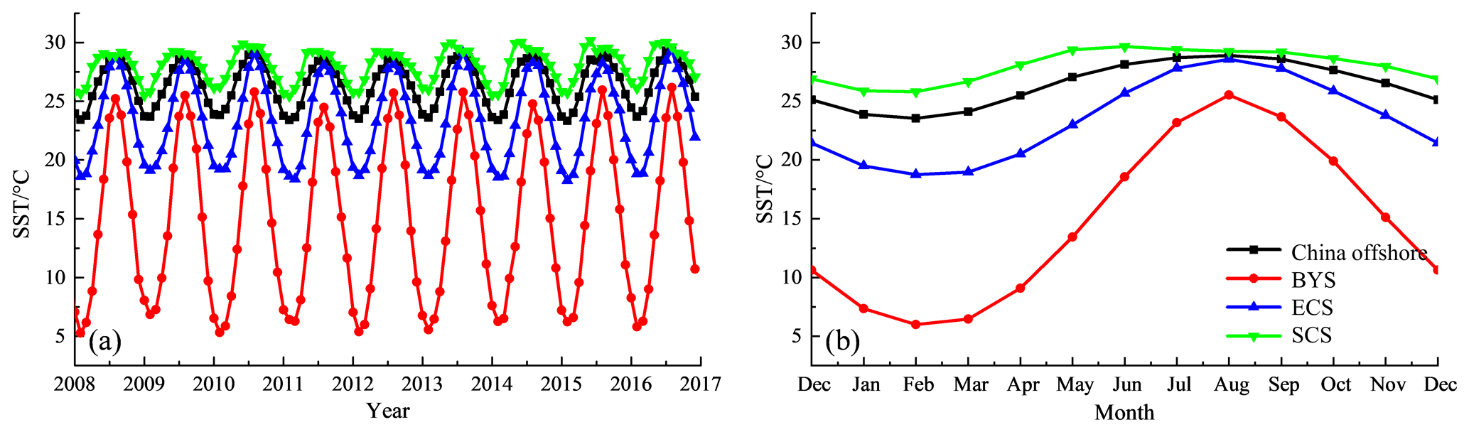
Figure 12 Long-term monthly mean SST of the marginal seas of China during 2008–2017: (a) yearly; (b) monthly. Black line: China offshore; red line: Bohai Sea and Yellow Sea (BYS); blue line: East China Sea (ECS); green line: South China Sea (SCS).

Table 2 Annual and seasonal SST characteristics of the study area in China offshore based on monthly data from 1988 to 2017.

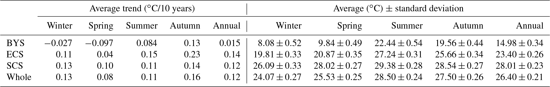
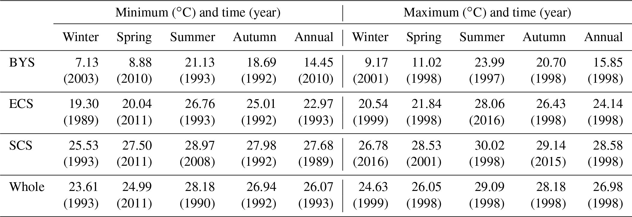
Table 3 Peak value and time of the annual and seasonal SST of the study area in China offshore based on monthly data from 1988 to 2017.

3.2 Spatial distribution of SST

Figure 6 shows the spatial distribution of the 30-year average SST for each month of 1988–2017. From the figure, we can find that the spatial distribution of annual average SST in each month is similar, and the SST is higher in the low-latitude (near the Equator) region and lower in the high-latitude region. In the low-latitude region, SST is more evenly distributed along the latitudes in January to April and November to December, and is higher in the south and lower in the north. From May to October, the distribution of SST along the latitude is tilted, showing the distribution characteristics as higher in the southwest and lower in the northeast, which is affected by the ocean circulation. In addition, as can also be seen in Fig. 6, in the low-latitude region, the SST range of change in different months is relatively small, between 27 and 33 ^∘C, the change range of 5 to 6 ^∘C. In the high-latitude region, the SST can be less than 3 ^∘C at the lowest and greater than 15 ^∘C at the highest, with a relatively large variation of more than 12 ^∘C.

Figure 7 shows the spatial distribution of seasonal and annual mean SSTs during the 1988–2017 period. As can be seen from the figure, the spatial distribution of average SST in each season and annually is similar, and similar to the monthly results (Fig. 6). In the low-latitude region, the SST is higher but in the high latitudes. SST is relatively low. Annual mean SST decreases with increasing latitude, with high temperature ranging from 26 to 28 ^∘C in the south and low temperature ranging from 3 to 6 ^∘C in the north, which is closely related to the solar radiation distribution in the deep-sea region. The isotherm is northeast–southwest oriented and the SST gradient increases as it gets closer to the mainland coastal line. It is obvious that the landmass effect in the wintertime has contributed to the tilting of the isotherms, which was pointed out by Bao et al. (2014).

Figure 8 shows the results of SST anomaly in three characteristic stages. Figure 8a shows the SST anomaly for the annual 1998 minus 1988–2017, Fig. 8b is the annual SST difference between the 10 years after 1998 (1998–2007) and the previous 10 years (1988–1997), and Fig. 8c is the SST anomaly for the last 10 years (2008–2017) and the past 30 years (1988–2017).

It can be seen that there was a significant positive anomaly across the past 30-year average in 1998 from Fig. 8a. The positive anomalies around 1.0 ^∘C are shown in a large area in China offshore, indicating that the SST is significantly warmer. In the southeast and northeast areas of the northwest Pacific, negative anomalies have occurred in this region, and the lowest is close to −0.6 ^∘C, indicating that the SST has cooled in this region. The SSTA in the northwest Pacific showed a trend of high in the west and low in the east. From the previous analysis, we found that this extremum is highly coincident with El Niño (Fig. 5). Therefore, it is likely that this phenomenon has been caused by the temperature difference and time difference caused by the transfer of high-temperature water in the northeast Pacific to the northwest Pacific under the combined influence of atmospheric circulation and ocean circulation.

It can be seen from Fig. 8b that the SST during the 10 years from 1998 to 2007 has significantly increased compared with the previous 10 years from 1988 to 1997. The positive anomaly is 0.4 to 0.8 ^∘C in the southern region of 40^∘ N. In the 10 years since 1998, the SST in the region has increased by 0.4 to 0.8 ^∘C over the previous 10 years. In the region between 45 and 60^∘ N, the effect is small and is maintained between −0.2 and 0 ^∘C, indicating that the SST in this region has not changed substantially or slightly.

Figure 8c shows the anomalous results of SST over the last 10 years (2008–2017) and relatively nearly 30 years (1988–2017). As can be seen from the figure, in addition to the Bohai Sea, the Yellow Sea and the southern region of Japan, there is a wide range of positive anomaly in other regions, and the past 10 years have increased on average in the past 30 years. From Fig. 4a and b, we have known that the increasing trend of SST over the past 30 years is around 3–4 times that of the rising trend of SST over the past 164 years. Therefore, the increasing trend of SST in the past 10 years is more significant, which is consistent with the results in Fig. 4c and Table 1.

3.3 Correlation between the SST and the atmospheric parameters

Based on monthly data from ERA-Interim, there is some correlation between SST and atmospheric parameters that has been shown in Fig. 9; all marked patterns are at the level of significance equal to 0.05. It can be seen from Fig. 9a that there is a non-significant correlation between SST and NAO but in China offshore and around the region. It shows a weak negative correlation between China offshore SST and NAO. The PDO is an important factor of climate change of the northwest Pacific, and it has a strong correlation with ENSO. The PDO has a great influence on the Asian monsoon and climate change in the northwest Pacific and is closely related to ENSO. The significant negative correlation between SST and PDO can be seen in Fig. 9b. The NINO3.4 index is usually used to indicate the intensity of the El Niño/La Niña events. So there is a significant negative correlation between SST and the NINO3.4 atmospheric parameter in Fig. 9d.

There is a significant positive correlation between SST and the Southern Oscillation Index (SOI) in Fig. 9c, which is a standardized index based on the observed sea level pressure differences between Tahiti and Darwin, Australia. The monthly correlation between SST and temperature at 2 m (T2) is high throughout the study region, most markedly (R > 0.95) over all of the northwest Pacific. The effect of T2 on SST is significant over 98 % of the study region in all seasons. This is in good agreement with the previous studies (Skliris et al., 2012; Shaltout and Omstedt, 2014). Similarly, based on monthly data, there is a significant positive correlation between SST and total column water (TCW) and precipitation (PRCP).

The maximum negative correlation between the effect of 10 m wind speed (WS10) on SST occurs in the southeastern northwest Pacific and is significant only in a small region. However, the direct correlation between V10 and SST is significant and positive over more of the northwest Pacific.

3.4 China offshore SST characteristics

China offshore is defined as the four sea areas of the Bohai Sea, Yellow Sea, East China Sea and South China Sea, and includes the Kuroshio Extension, the part of northwest Pacific and the sea surrounding Japan in this study, which is defined as the offshore region of 5–41^∘ N and 105–130^∘ E. The changes in the average SST in the Yellow Sea and the Bohai Sea are very similar, so we analyze the two sea areas together. Therefore, the region is further divided into three subregions: Bohai Sea and Yellow Sea (BYS, 35–41^∘ N and 117–127^∘ E), East China Sea (ECS, 22–35^∘ N and 120–130^∘ E) and South China Sea (SCS, 5–22^∘ N and 105–120^∘ E).

Figure 11 shows the spatial distribution of seasonal and annual mean SSTs in China offshore during the 1988–2017 period. Annual mean SST decreases with increasing latitude, with high temperature ranging from 26 to 28 ^∘C in the south and low temperature ranging from 14 to 16 ^∘C in the north, which is closely related to the solar radiation distribution in the offshore region. The isotherm is northeast–southwest oriented and the SST gradient increases as it gets closer to the mainland coastal line. It is obvious that the landmass effect in the winter has contributed to the tilting of the isotherms, which was pointed out by Bao et al. (2014). The ECS exhibits the largest temperature gradient, and the SCS in the tropical zone exhibits the lowest temperature gradient.

The monthly mean surface temperature changes over the past 10 years in the three regions (BYS, ECS and SCS) and the whole sea area (China offshore) are shown in Fig. 12. Figure 12a shows the year-by-year variation of SST in different regions in the last 10 years, and Fig. 12b shows the monthly SST variations in different regions in the past 10 years. The change variability of SST in different regions is basically synchronized. The minimum temperature basically occurs in February and the warmest occurs in August. The fluctuation range of SST in BYS is the largest, basically between 5 and 22 ^∘C, from 18 to 27 ^∘C in the East China Sea, and the smallest fluctuations are in the South China Sea, maintained at a range of 26 to 29 ^∘C. There are large differences between the mean and standard deviation in different regions.

Table 2 shows the annual and seasonal SST characteristics of the study area in China offshore based on monthly data from 1988 to 2017. It can be found that in addition to the winter and spring in the BYS, the SST in each season of other regions shows an increasing trend from the table. The average increasing trend of SST during 1988 to 2017 in BYS is 0.015 ^∘C/10 years, 0.14 ^∘C/10 years for the ECS, 0.12 ^∘C/10 years for the SCS and 0.12 ^∘C/10 years for the whole China offshore area, respectively, and all the trends are significant at the 99 % confidence level. From the point of average annual SST, the SST in the South China Sea is the highest, reaching 28.01 ^∘C, followed by the East China Sea with 23.4 ^∘C, the lowest in the Bohai Sea and the Yellow Sea is 14.98 ^∘C, and the SST in the whole China offshore area is 26.4 ^∘C. Table 3 shows the peak value and time of the annual and seasonal SST of the study area in the China offshore area based on monthly data from 1988 to 2017. In the past 30 years, colder SST occurs in 1989, 1990, 1992, 1993, 2003, 2008, 2010 and 2011. Warmer SST occurs in 1997, 1998, 1999, 2001, 2015 and 2016.

4 Conclusions

The northwest Pacific sea surface variability is affected by a combination of oceanic and atmospheric processes and displays significant regional and seasonal behavior. Monthly SST datasets based on ERSST 3b (1854–2017, 164 years) and OISST V2 (1988–2017, 30 years) are used to make some long-term temporal and spatial variability statistics. The following conclusions can be drawn from the analysis.

In the last 164 years, SST in the northwest has gradually increased, with an increasing trend of 0.033 ^∘C/10 years. Especially in the past 30 years, the increasing trend of SST reached 0.132 ^∘C/10 years, and the increasing trend of SST reached 0.306 ^∘C/10 years in the last 10 years. The trend of the SST varies seasonally. The increasing trends in winter and autumn are 0.124 and 0.146 ^∘C/10 years, respectively, which are greater than those in spring and summer, with 0.075 and 0.107 ^∘C/10 years, respectively. There was an SST extremum point that occurred around 1998; the average annual SST for the 10 years after 1998 increased by 0.3 ^∘C over the previous 10 years. It has been found that the change of SST/SSTA in the northwest Pacific is closely related to the ENSO through the statistical analysis of the NINO3.4 index and SST/SSTA.

From the perspective of spatial distribution, the annual mean SST decreases with increasing latitude, with high temperatures ranging from 27 to 33 ^∘C in the south and low temperatures ranging from 3 to 15 ^∘C in the north. The SST is higher in the low-latitude (near the Equator) region and lower in the high-latitude region. In the low-latitude region, SST is more evenly distributed along the latitudes in November to April, but from May to October, the distribution of SST along the latitude is tilted, showing the distribution characteristics as higher in the southwest and lower in the northeast, which is affected by the ocean circulation.

There are many correlations between the SST and some climate indices and atmospheric parameters, such as PDO, SOI, NINO3.4, total water vapor column (TCW), T2, sea level pressure (SLP), PRCP and wind speed at 10 m (U10, V10 and WS10). Two very significant positive correlations between SST and T2, TCW have been found, of which the correlation coefficient between SST and T2 exceeded 98 %. PDO and NINO3.4 are negatively correlated with SST, and the correlation between other indices and parameters and SST is weak.

The whole China offshore area was divided into three sections to analyze its spatial variability in different regions, which are the BYS, ECS and SCS. The SST in the BYS is coolest, with a range from 5 to 22 ^∘C, and the warmest in the SCS, with a range from 26 to 29 ^∘C. It can be seen from the statistical data that, in addition to the winter and spring in the BYS, SST in other regions and at other times had shown a warming trend. In the past 30 years, the trend of SST increase of BYS was 0.015 ^∘C/10 years, while those of ECS and SCS were 0.14 and 0.12 ^∘C/10 years, respectively.