the Creative Commons Attribution 4.0 License.
the Creative Commons Attribution 4.0 License.
 | 03 Jul 2020
Ventilation of the northern Baltic Sea
Thomas Neumann
Herbert Siegel
Matthias Moros
Monika Gerth
Madline Kniebusch
Daniel Heydebreck
The Baltic Sea is a semi-enclosed, brackish water sea in northern Europe. The deep basins of the central Baltic Sea regularly show hypoxic conditions. In contrast, the northern parts of the Baltic Sea, the Bothnian Sea and Bothnian Bay, are well oxygenated. Lateral inflows or a ventilation due to convection are possible mechanisms for high oxygen concentrations in the deep water of the northern Baltic Sea.
In March 2017, conductivity–temperature–depth (CTD) profiles and bottle samples, ice core samples, and brine were collected in the Bothnian Bay. In addition to hydrographic standard parameters, light absorption has been measured in all samples. A complementary numerical model simulation provides quantitative estimates of the spread of newly formed bottom water. The model uses passive and age tracers to identify and trace different water masses.
Observations indicate a recent ventilation of the deep bottom water at one of the observed stations. The analysis of observations and model simulations shows that the Bothnian Bay is ventilated by dense water formed due to mixing of Bothnian Sea and Bothnian Bay surface water initializing lateral inflows. The observations show the beginning of the inflow and the model simulation demonstrates the further northward spreading of bottom water. These events occur during wintertime when the water temperature is low. Brine rejected during ice formation barely contributes to dense bottom water.
Please read the corrigendum first before continuing.
-
Notice on corrigendum
The requested paper has a corresponding corrigendum published. Please read the corrigendum first before downloading the article.
-
Article
(13870 KB)
-
The requested paper has a corresponding corrigendum published. Please read the corrigendum first before downloading the article.
- Article
(13870 KB) - Full-text XML
- Corrigendum
- BibTeX
- EndNote


The Baltic Sea is a semi-enclosed marginal sea in northern Europe with a positive freshwater budget (e.g., Lass and Matthäus, 2008), and as a result, the surface salinity ranges from 14 g kg−1 (south) to 2.5 g kg−1 (north). Due to its hydrographic conditions, an estuarine-like circulation is established and a strong and permanent vertical density stratification occurs. These hydrographic conditions set the prerequisites for vulnerability to hypoxia and anoxia below the pycnocline. In general, a ventilation is only possible by lateral intrusions of oxygenated water of a sufficiently high density which allows this water to enter depths below the pycnocline. Indeed, the modern Baltic Sea shows wide areas of hypoxia in its central part. However, the northern parts of the Baltic Sea, the Bothnian Sea and Bothnian Bay, are characterized by well-oxygenated bottom water, although for the last decades a decreasing oxygen concentration was reported (Raateoja, 2013).
The common prerequisite for deep water renewal due to inflows (cascading) is a sufficient lateral density gradient and slope of the ocean floor. A comprehensive summary of possible mechanisms producing density gradients and theoretical aspects for the initiation of cascades is given in Shapiro et al. (2003). In the case of the northern Baltic Sea, salinity difference is the main driver for lateral density gradients. Small temperature differences close to the temperature of maximum density during winter do not have a significant effect on density compared to the effect of observed salinity gradients.
The bathymetric structure of the Baltic Sea is characterized by connected basins separated by shallow sills (Fig. 1). Cascades of descending water may be initiated if the density of water over the sills exceeds the density of the adjacent basin sufficiently. The depth of final interleaving depends on the lateral density difference and the entrainment on its way by the dense water plume. Stigebrandt (1987) estimates the entrainment into dense bottom currents of the Baltic Sea as a function of the slope (Eq. 3.12 in Stigebrandt, 1987). For the central Baltic Sea, major Baltic inflows (e.g., Mohrholz, 2018) are the dominating process for bottom water ventilation. The origin of the new water mass is the North Sea; it leaves the surface in the western Baltic Sea and spreads northward as a dense bottom plume.
Marmefelt and Omstedt (1993) investigated processes for deep water renewal in the northern Baltic Sea and concluded that inflows of dense water are the main process rather than vertical convection. In contrast to major Baltic inflows in the central Baltic Sea, those inflows into the Bothnian Sea and Bothnian Bay originate from surface water of the Sea of Åland and Northern Quark (Fig. 1), respectively. Therefore, this inflowing water is saturated with oxygen, and these events may occur more often than major Baltic inflows. Other possible processes, thermal and haline convection, have been assessed as highly unlikely. However, Marmefelt and Omstedt (1993) also noticed that more observations from the Bothnian Bay are needed during wintertime.
Geological studies from the Baltic Sea (Moros et al., 2020) indicate that deep water formation cause widespread resuspension and transport of sediment during colder climatic periods. Sediment contourite drifts are prominent in depths greater than 200 m in the Gulf of Bothnia and the northern Baltic Proper, and therefore cold conditions appear to favor dense water production. In fact, one cannot compare today's climate with conditions during the Little Ice Age (e.g., Kabel et al., 2012), when widespread sea ice dominated the Baltic Sea in winter. Today, the Baltic Sea shows conditions where sea ice appears regularly and surface water is cooled down to freezing temperature in the Bothnian Bay only. However, a mechanistic description of the detected sediment redistribution is still lacking.
In addition to dense water formation due to saline water from adjacent seas as described by Marmefelt and Omstedt (1993), dense water also can be formed due to brine from sea ice formation. It is an usual phenomenon in Arctic and Subarctic regions. Dense and saline water masses are generated at hotspots of sea ice production, the polynyas. But also melting sea ice can produce considerable salt fluxes into the ocean. Peterson (2018) observed a substantial salt loss in Arctic sea ice due to warming. The explanation is an increased permeability which allows gravity drainage. The general idea of new water mass formation due to brine is that dense water is generated at the shelf and then a gravity driven flow can reach deeper regions of the ocean (Aagaard et al., 1981; Ivanov et al., 2004; Skogseth et al., 2008). However, due to the rough weather conditions, experimental studies are sparse.
Sea ice in the northern Baltic Sea shows a considerably lower bulk salinity compared to sea ice in the Arctic ocean due to the low seawater salinity. Usually, values less than 1 g kg−1 have been observed (e.g., Meiners et al., 2002; Granskog et al., 2005). In addition, Baltic Sea ice can consist of up to 35 % metamorphic snow (Granskog et al., 2006), and therefore the brine volume in Baltic Sea ice is smaller than that in Arctic sea ice. However, brine salinity is comparable (Assur, 1958).
In this study, we present data from a 2 d long expedition with the RV Maria S. Merian in the sea-ice-covered Bothnian Bay, the most northern basin of the Baltic Sea (Fig. 1), in March 2017. Samples from sea ice, brine, and water column profiles and bottle samples have been taken and analyzed. Furthermore, we performed numerical model studies to reproduce the campaign and to provide additional data for analysis. The aim of this study is to identify relevant processes ventilating the deep water of the Bothnian Bay and to quantify the importance of brine for dense water formation.

Figure 1Bathymetry of the Baltic Sea showing names of different geographic regions we will use in the text. The map was created using the software package GrADS 2.1.1.b0 (http://cola.gmu.edu/grads/, last access: 19 June 2020), using published bathymetry data (Seifert et al., 2008).
The Baltic Sea ice season of 2016–2017 was mild with a maximum ice extent of 80 000 km2 reached on 12 February (Baltic Icebreaking Management, 2017). Sea ice samples and water samples in the northern Baltic Sea, the Bothnian Bay and the Bothnian Sea, were taken during the expedition MSM62 with RV Maria S. Merian between 12 and 13 March 2017. During this time, the Bothnian Bay was well covered by sea ice (Fig. 2).
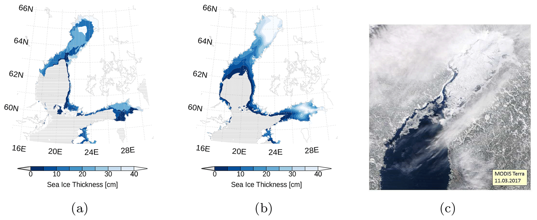
Figure 2Sea ice thickness (a) at 12 March 2017 in the Bothnian Sea and the Bothnian Bay. Data are based on the Finnish Meteorological Institute's ice charts and freely distributed by the Copernicus Marine Environment Monitoring Service (marine.copernicus.eu). Panel (b) is the same as (a) but from our model simulation. Sea ice coverage (c), quasi-true color image derived from MODIS at 11 March 2017. The map in panels (a) and (b) was created using the software package GrADS 2.1.1.b0 (http://cola.gmu.edu/grads/, last access: 19 June 2020).
For sea ice sampling, the RV sailed into the ice cover until it was surrounded by pack ice. In a distance of about 50 m from the RV, ice core samples were taken. Near the ice core stations, shipborne conductivity–temperature–depth (CTD) measurements were performed. For this purpose, the RV steamed a short distance to be freed from surrounding sea ice and the CTD probe could be lowered undisturbed. Names and locations of stations are shown in Fig. 3.
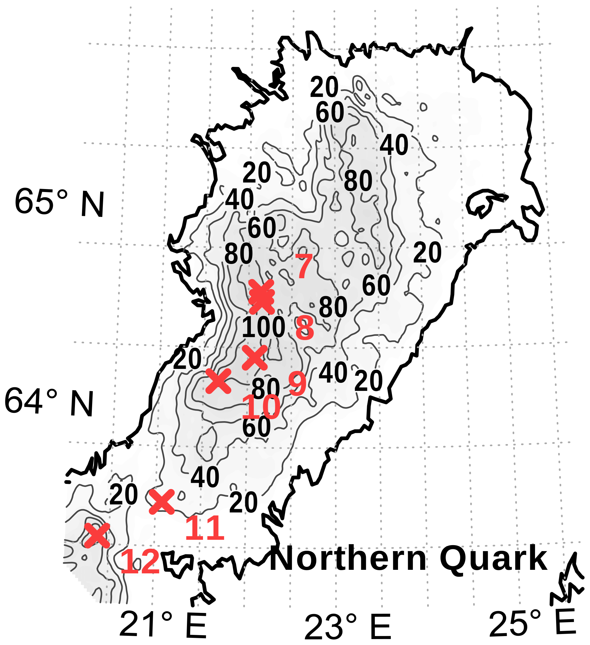
Figure 3Locations of stations (red crosses) in the Bothnian Bay (stations 7 to 10), the Northern Quark (station 11), and the Bothnian Sea (station 12). Stations 7, 11, and 12 were CTD-only stations. At stations 8, 9, and 10, sea ice and brine samples were taken. Near stations 9 and 10 also a CTD cast was performed. The map was created using the software package GrADS 2.1.1.b0 (http://cola.gmu.edu/grads/, last access: 19 June 2020), using published bathymetry data (Seifert et al., 2008).
2.1 Ice core sampling
With the aid of an ice corer, three to four sea ice cores were taken at each station. The lengths of the cores varied from 0.3 to 0.6 m. Obvious snow and loose parts were removed from the surface. In addition, holes approximately half the depth of the ice thickness were drilled; the ice core was removed and brine draining from the ice accumulated in the hole. After about 30 min, we took the brine sample from the borehole with a pipette. Brine could be collected at two stations (stations 8 and 10; Fig. 3).
Onboard, the ice cores were cut into two or three segments depending on the total length and structure of the ice core. Snow was removed from the ice fragments and then the ice was melted for further analysis. After salinity estimations, the meltwater was filtered and samples were prepared for analysis of yellow substances. Salinity of the ice cores and brine was measured with a hand-held CTD (see Sect. 2.2). Due to the size of the sensor pack, a small sample volume of about 100 mL was sufficient. In addition, selected salinity samples (Table 1) were measured with a Guildline’s Autosal 8400B laboratory salinometer. The accuracy of the Autosal is better than 0.002 equivalent practical salinity units (PSUs).
2.2 Water column sampling
A CTD system “SBE 911plus” (Sea-Bird Electronics) was used to measure pressure, temperature, conductivity, oxygen, fluorescence chlorophyll, back-scattering turbidity, and CDOM (colored dissolved organic matter, fluorescence method 370∕460 nm ex ∕ em). For temperature, conductivity, and oxygen, two sensors were installed to ensure a high standard of data quality. A benthic altimeter delivered the bottom distance. Additionally, the CTD probe was equipped with an SBE 32 water sampler with 13 free-flow bottles of 5 dm3 volume. The CTD was always put for at least 3 min at 10 m depth into the water before the cast started in order to remove air bubbles from the pumping system and water samplers. The CTD was lowered at 0.3 to 0.5 m s−1.
We recalibrated each oxygen profile with the assumption that the upper 5 m are well mixed and saturated with oxygen, i.e., a small offset has been applied to all oxygen profiles. This assumption was made on the basis of temperature and salinity profiles (Fig. 7) which are homogeneous in the upper layer.
After sea ice coring, a hand-held CTD was deployed through the borehole to measure the water column directly below the sea ice. For these measurements, a CTD48M by Sea & Sun Technology was used. The CTD48M is a very small multi-parameter probe for precise online measurements. Data are stored internally and can be downloaded after the mission. Due to the low weight of 1.2 kg and the small housing diameter of 48 mm, the probe is well suited for deployments in a borehole.
The probe was equipped with a pressure, temperature, and conductivity sensor. The pressure transducer is a piezoresistive full bridge. For temperature measurements, a platinum resistor with nominal 100 ohm resistance at 0 ∘C (PT100) is used. Conductivity is measured by a cell which consists of a quartz glass cylinder with seven platinum-coated ring electrodes.
All shown quantities, like conservative temperature, absolute salinity, freezing temperature, density, etc., have been computed following the TOES-10 manual (ICO et al., 2010) from measured in situ data.
2.3 Seawater optics
For the determination of the spectral absorption of dissolved organic substances (CDOM, yellow substances), seawater was filtered under low vacuum through Whatman GF/F glass fiber filters (pore size approximately 0.7 µm). The filtered water was measured in a 10 cm cuvette using a dual-beam Perkin Elmer Lambda 2 instrument in the wavelength range between 300 and 750 nm with increments of 1 nm. Milli-Q water was the reference. Comparisons between Whatman GF/F and membrane filters with a pore size of 0.2 µm did not deliver significant differences for the area of investigation.
The spectral absorption coefficients ay(λ) were calculated according to Kirk (1994):
where A(λ) is the spectrophotometer absorbance at wavelength λ, l is the optical path length, and A(720 nm) is the baseline correction. The spectral dependence of CDOM absorption is characterized by an exponential increase to shorter wavelengths with a maximum in the UV spectral range and can be described according to Jerlov (1976) and Kirk (1994) by the following equation:
where ay(λ) is the absorption coefficient at the wavelength λ, λ0 is the reference wavelength, and s is the spectral slope for the exponential dependence. The absorption coefficient at 440 nm is used for comparisons.
2.4 Model simulations
For the analysis of different water masses, we use a three-dimensional numerical model of the Baltic Sea. The model code is Modular Ocean Model (MOM) 5.1 (Griffies, 2004) adapted for the Baltic Sea. The horizontal resolution is 1 nautical mile. Vertically, the model is resolved into 152 layers with a layer thickness of 0.5 m at the surface and gradually increasing with depth up to 2 m.
The circulation model MOM5.1 is coupled with a sea ice model (Winton, 2000) which accounts for ice formation and drift. Brine rejection is simulated by a sea surface salt flux. With a prescribed bulk ice salinity, the surplus salt is rejected immediately during freezing. Due to the numerics of ocean models (grid spacing on the order of kilometers and the hydrostatic approximation), the models cannot resolve microscopic processes like brine release. Therefore, we implemented a parametrization for the subgrid-scale convection of brine proposed by Nguyen et al. (2009). The parametrization distributes rejected brine within the mixed layer vertically simulating convective salt plumes. We used the calibration of Nguyen et al. (2009) for this study.
For earmarking water masses, we used the capability of the MOM5.1 model to define passive tracers which are set to unity at the surface at each model time step. Two passive tracers, each for the Bothnian Bay and the Bothnian Sea, are set up. Figure 4 shows the horizontal and vertical extent of the passive tracers. Due to vertical mixing, the passive tracer is evenly distributed over the mixed layer after a few days of simulation. In addition, we have defined an age tracer for each passive tracer. The age of the corresponding tracer is set to zero at the surface at each model time step and otherwise increases with each time step. Furthermore, we defined a brine tracer for each passive tracer region. The brine tracer represent the salinity rejected from sea ice during freezing. That is, the brine tracer is the salinity fraction due to brine.
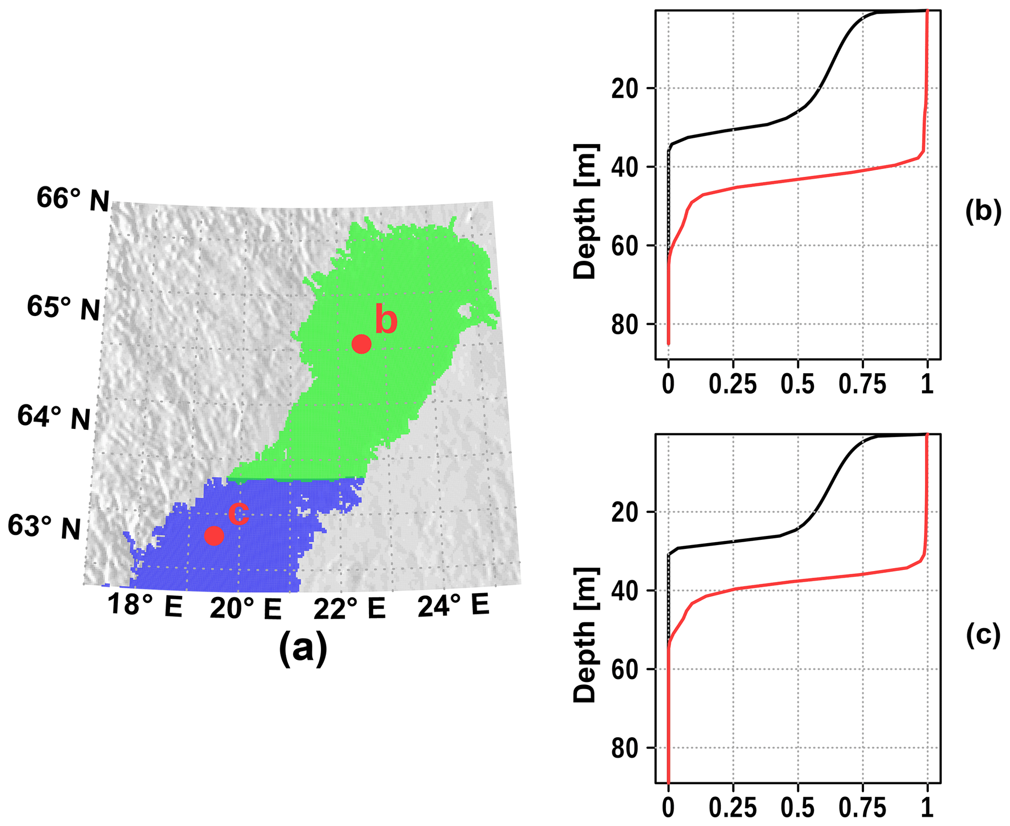
Figure 4Initializing of the surface tracer in the northern Baltic Sea: horizontal extent (a) of Bothnian Sea surface tracer (blue) and Bothnian Bay surface tracer (green), and vertical extent (b, c). The vertical profiles after 1 d (black) and after 10 d (red) are shown.
The model has been forced by meteorological data from the coastDat-2 data set (Geyer and Rockel, 2013). We run the model from 1948 to 2018, and the passive tracers have been activated in January 2017. In many studies, the model has been successfully applied (e.g., Neumann, 2010; Neumann et al., 2015). An assessment of the model performance in the northern Baltic Sea is given in Appendix A.
3.1 Sea ice samples
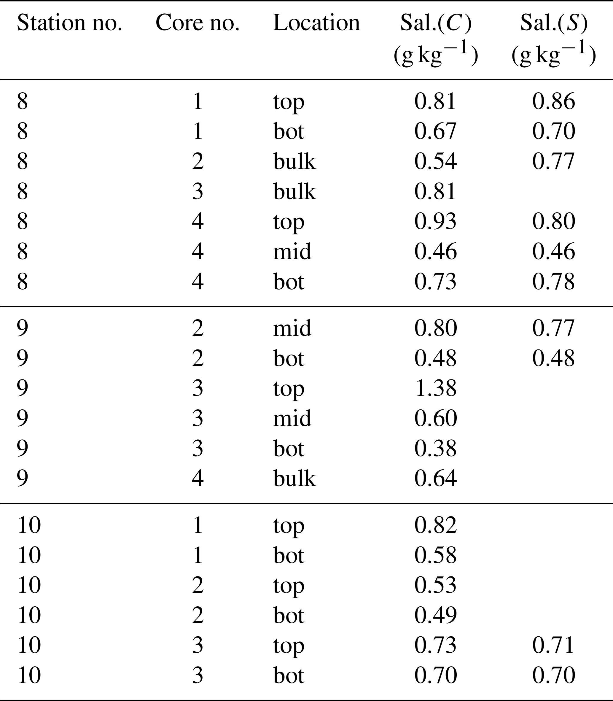
Bulk salinity of the sea ice cores is summarized in Table 1. Salinity measurements with the salinometer and the mini CTD of the melted ice core water are very close and therefore, the mini CTD measurements appear to be reliable. The mean bulk salinity of our sea ice samples amount to about 0.6 g kg−1 and the sea surface salinity at the ice core stations showed values between 2.95 and 3.0 g kg−1.
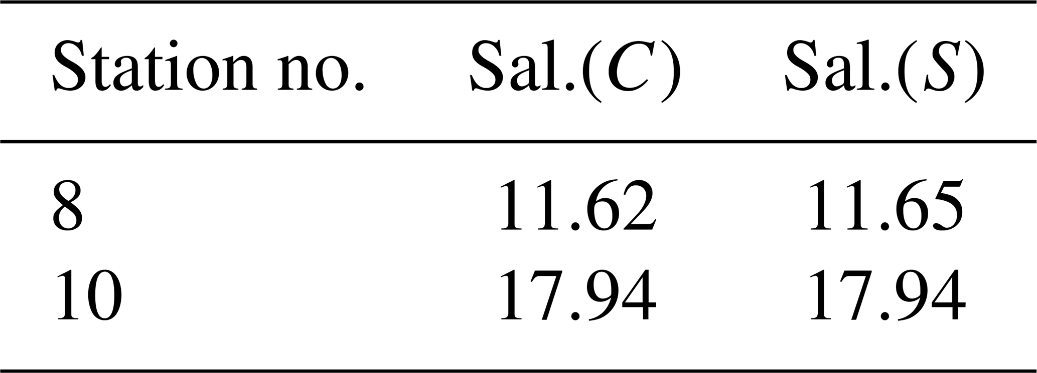
Table 1Ice core samples from stations 8, 9, and 10. Location shows which part of the core is used for analysis. Top, mid, and bot are the upper, middle, and lower parts of the ice core, respectively. Bulk is for the whole ice core. Sal.(C) and Sal.(S) are the absolute salinity measured with mini CTD and salinometer, respectively.
The sampled brine volume at station 9 was too small for further analysis. Brine salinity for stations 8 and 10 is listed in Table 2. As for the ice core samples, salinity measurements with mini CTD and salinometer are very close to each other. The mean brine salinity is about 15 g kg−1.
Table 2Brine samples from stations 8 and 10. Sal.(C) and Sal.(S) are the absolute salinity measured with mini CTD and salinometer, respectively.
Altogether, the sea ice measurements can be summarized as follows. The mean sea ice bulk salinity of our samples is about 0.6 g kg−1. Taking into account a sea surface salinity of 3.0 g kg−1, 2.4 g of salt are rejected from 1 kg frozen seawater into the water column, while the rejected brine shows a salinity of 15 g kg−1.
The spectral absorption of CDOM was measured at samples from three ice stations (8, 9, 10; Fig. 3). Surface water samples from ice holes and CTD rosette were compared with brine and water from different melted ice layers – mainly top, middle, and bottom layers. The absorption shows strong differences between ice samples, surface water, and brine. Highest values were measured in brine and lowest values in ice water, while only small differences were found within the different groups. Absorption measurements of brine was possible only at station 10 due to low brine volumes sampled at stations 8 and 9. The measured spectra are shown in Fig. 5.
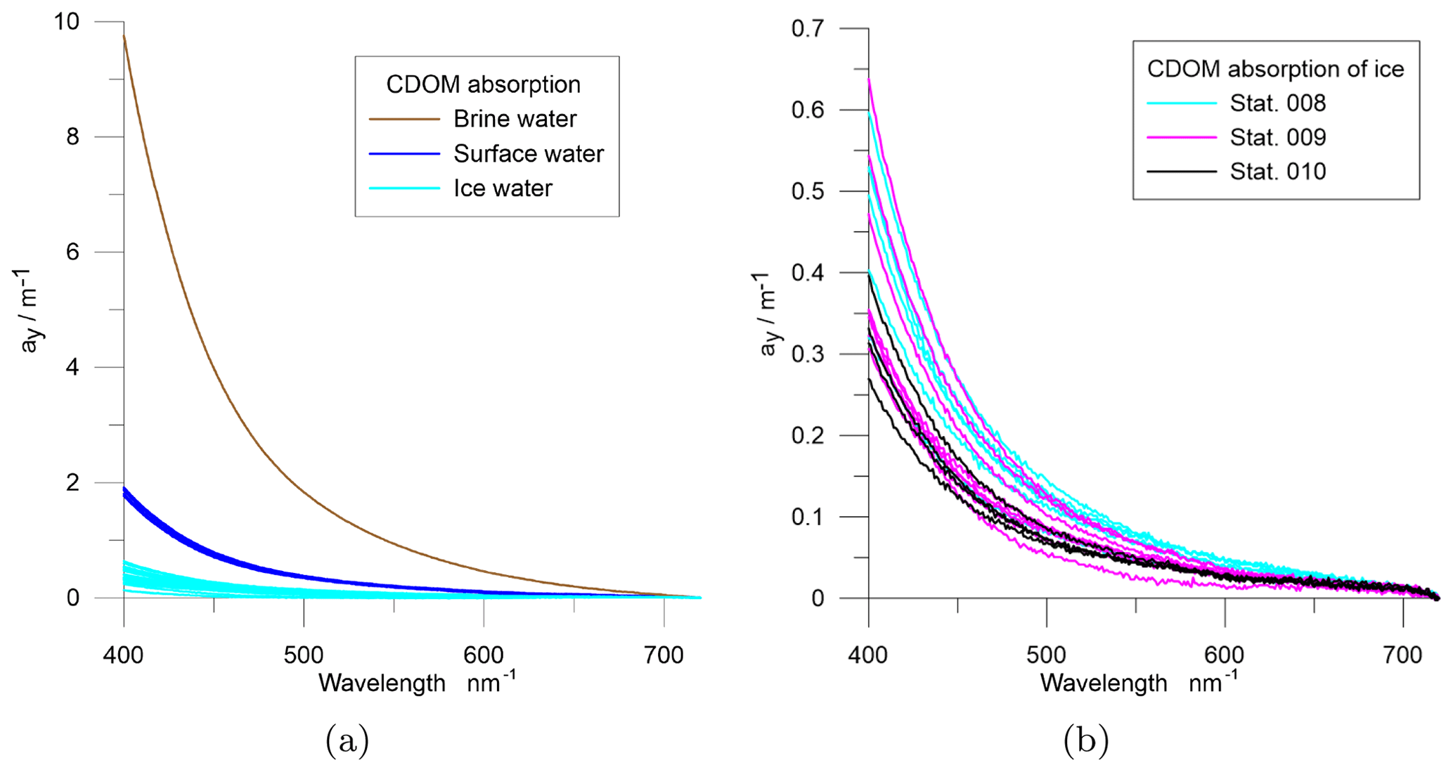
Figure 5Spectral absorption at the sea ice stations including surface water from ice holes and CTD-rosette samples, brine, and water from different melted ice core sections at stations 8, 9, and 10 (Fig. 3). Panel (b) shows melted sea ice absorption separately.
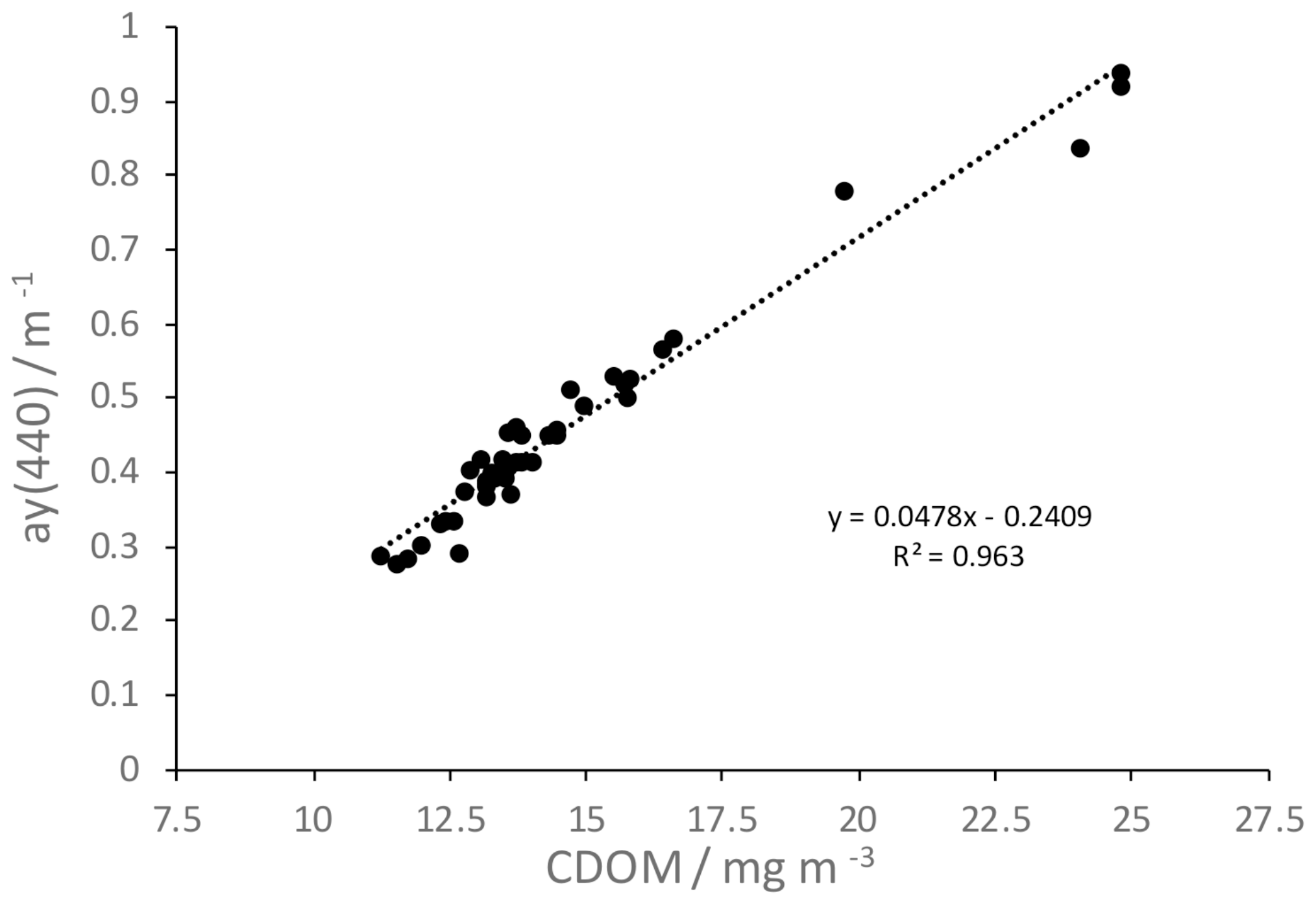
Figure 6Linear regression between CDOM absorption at 440 nm and CDOM content derived from Wetlabs CDOM fluorescence sensor.
For the relation between CDOM absorption at 440 nm and CDOM content estimated from Wetlabs CDOM fluorescence sensor (Sect. 2.2), we derived a linear regression (Fig. 6). This regression can be used to calculate CDOM absorption from CDOM content, and vice versa.
CDOM concentrations at station 10, estimated from the relation in Fig. 6, are listed in Table 3. Similar to salt, CDOM concentration increases in brine due to sea ice formation. However, the increase for salt (17.94 g kg−1 to 2.95 g kg−1) is stronger than the increase for CDOM (103.99 mg m−3 to 23.8 mg m−3). That means, relatively more CDOM remains in sea ice. Müller et al. (2011, 2013) showed that CDOM in Baltic Sea ice is enriched compared to salt with an enrichment factor of up to 39 %. Our estimates for station 10 show an enrichment of 50 % to 70 %.
Table 3CDOM absorption and CDOM concentration in brine, water, and sea ice at station 10.

3.2 Water column samples
Figure 7 shows temperature, salinity, oxygen, and CDOM profiles from stations 7, 9, 10, and 11 (see Fig. 3 for locations).
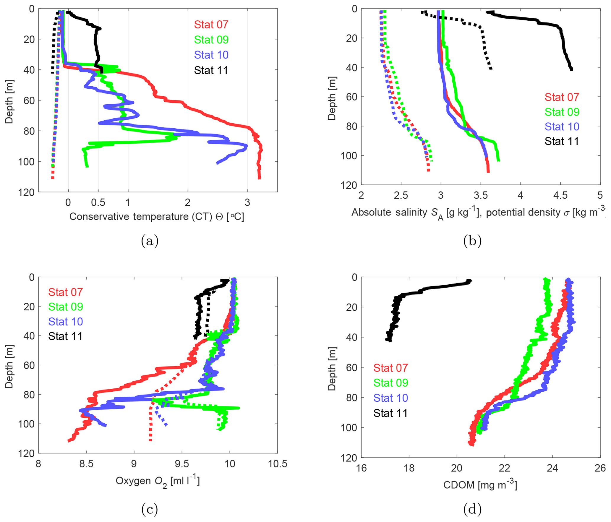
Figure 7Shipborne CTD profiles at stations 7, 9, 10, and 11 (Fig. 3) for conservative temperature (a), absolute salinity (b), oxygen (c), and CDOM (d). Dotted lines show the freezing temperature (a), the potential density (b), and the saturation oxygen concentration (c).
In the Bothnian Bay, temperature near the surface is close to the freezing temperature. The density profiles suggest that the upper 20 to 30 m are well mixed. At the Northern Quark (station 11), stratification starts just below the surface, presumably due to water from the Bothnian Bay which is continuously mixed with the underlying water from the Bothnian Sea.
A weak stratification also existed below the sea ice measured with the hand-held mini CTD through the bore holes. Temperature stratification starts at a depth of about 25 m. We do not show the data since they are very similar to the data measured with the shipborne CTD.
At all Bothnian Bay stations, temperature and salinity increase with depth below the mixed layer while oxygen is decreasing, either due to salinity and temperature increase (still close to saturation concentration) or due to oxygen consumption. There is an exception at station 9, where a 20 m thick layer above the ocean floor is well oxygenated, even slightly oversaturated, showing a very low temperature. We assume that this water mass was formed from water which recently was in contact with the sea surface and therefore, indicate a ventilation event of the bottom water at station 9. To identify a possible genesis of this bottom water, we analyzed the temperature–salinity (TS) properties based on our CTD measurements.
The TS characteristics are shown in Fig. 8. In addition to the Bothnian Bay stations, we included station 12 from the northern Bothnian Sea. Only data points with oxygen concentrations close to saturation, and from station 12 only the upper 20 m, are included. This restriction is justified by the fact that the water mass of interest, the bottom water at station 9, is saturated with oxygen and the Northern Quark sill depth is shallower than 20 m and constrains inflows from the Bothnian Sea.
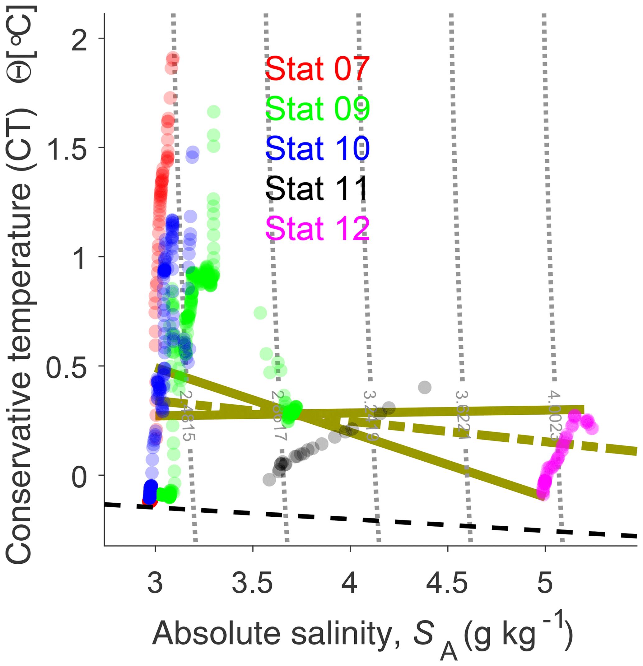
Figure 8TS diagram for stations 7, 9, 10, 11, and 12 (Fig. 3). Gray dotted lines show the density. Greenish solid and dash-dotted lines show mixing lines for station 9 bottom water from Bothnian Bay and Bothnian Sea surface water, and from Bothnian Bay water and brine, respectively. Brine is outside the figure with SA of 15 g kg−1 and CT of . Only data points with oxygen concentration close to saturation are considered. For station 12, data points are restricted to a depth shallower than 20 m. The dashed black line is the freezing temperature. Stronger opacity of the data points refers to a higher number of data.
The bottom water from station 9 (well oxygenated) is roughly in the middle of Fig. 8, where mixing lines are crossing. The light greenish, solid lines indicate mixing of water masses from the Bothnian Sea and Bothnian Bay which potentially could have contributed to the bottom water at station 9. The surface water in the Bothnian Bay is close to freezing temperature down to 40 m depth (Fig. 7) and not a candidate for forming the bottom water of station 9. The northern Bothnian Sea surface water is at the other end (right side) of the mixing lines. The greenish dash-dotted line in Fig. 8 is the mixing line, if brine and Bothnian Bay water would form station 9 bottom water. Brine properties have been chosen according to our observations and (freezing temperature). Based on the temperature constraints given by TS characteristics, we suggest that recent Bothnian Bay surface water was not contributing to station 9 bottom water.
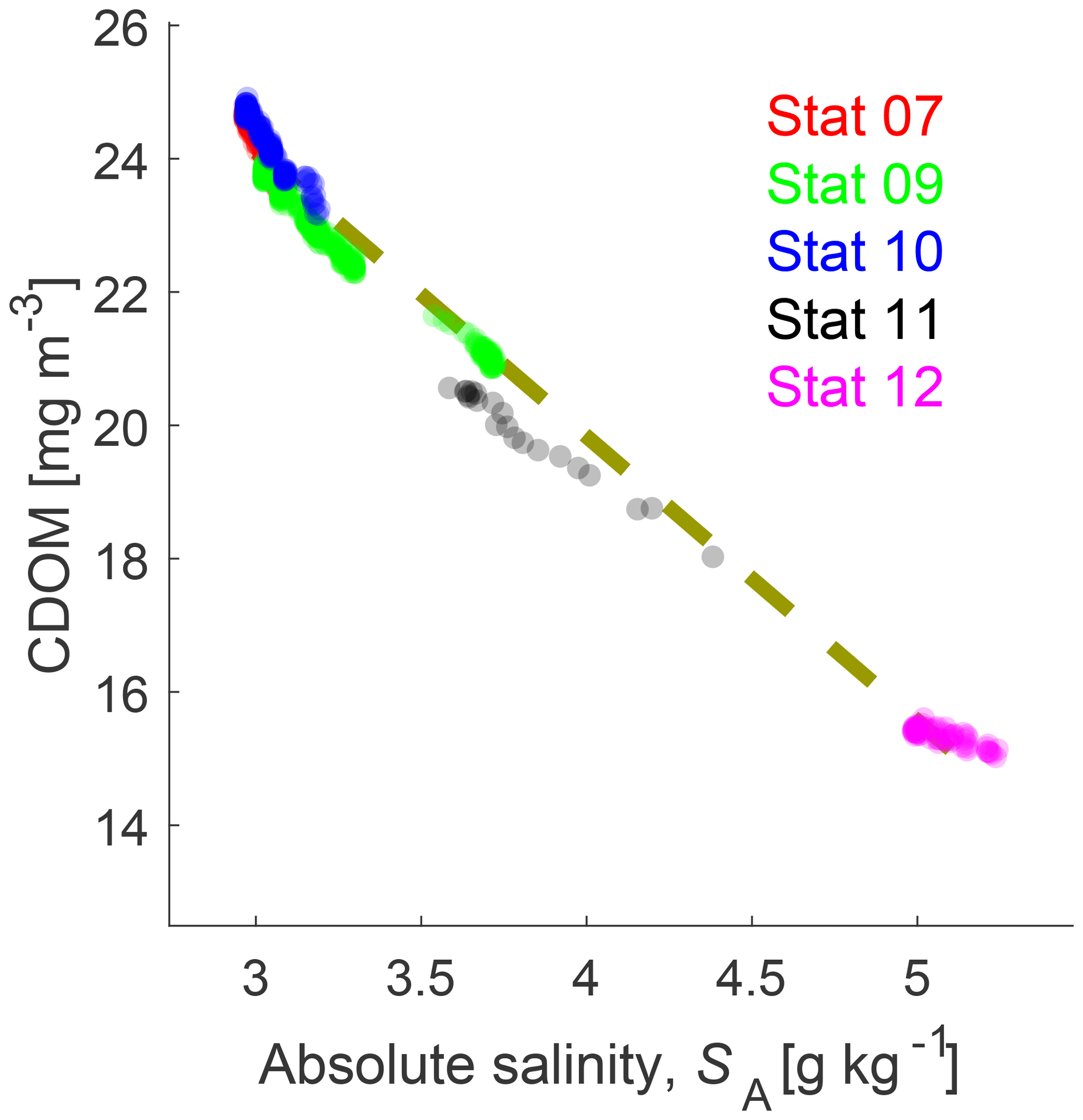
Figure 9Salinity–CDOM diagram. The dashed line is the mixing line. Stronger opacity of the data points refers to a higher number of data. Data of station 7 are mostly covered by station 9 and 10 data.
The salinity–CDOM relationship is shown in Fig. 9. The main source for CDOM in the northern Baltic Sea are yellow substances carried by rivers into the Baltic Sea. Yellow substances in the Baltic Sea are relatively refractory, and therefore a linear CDOM salinity relation exists (e.g., Harvey et al., 2015). All oxygen saturated water masses are along the mixing line.
3.3 Model simulations
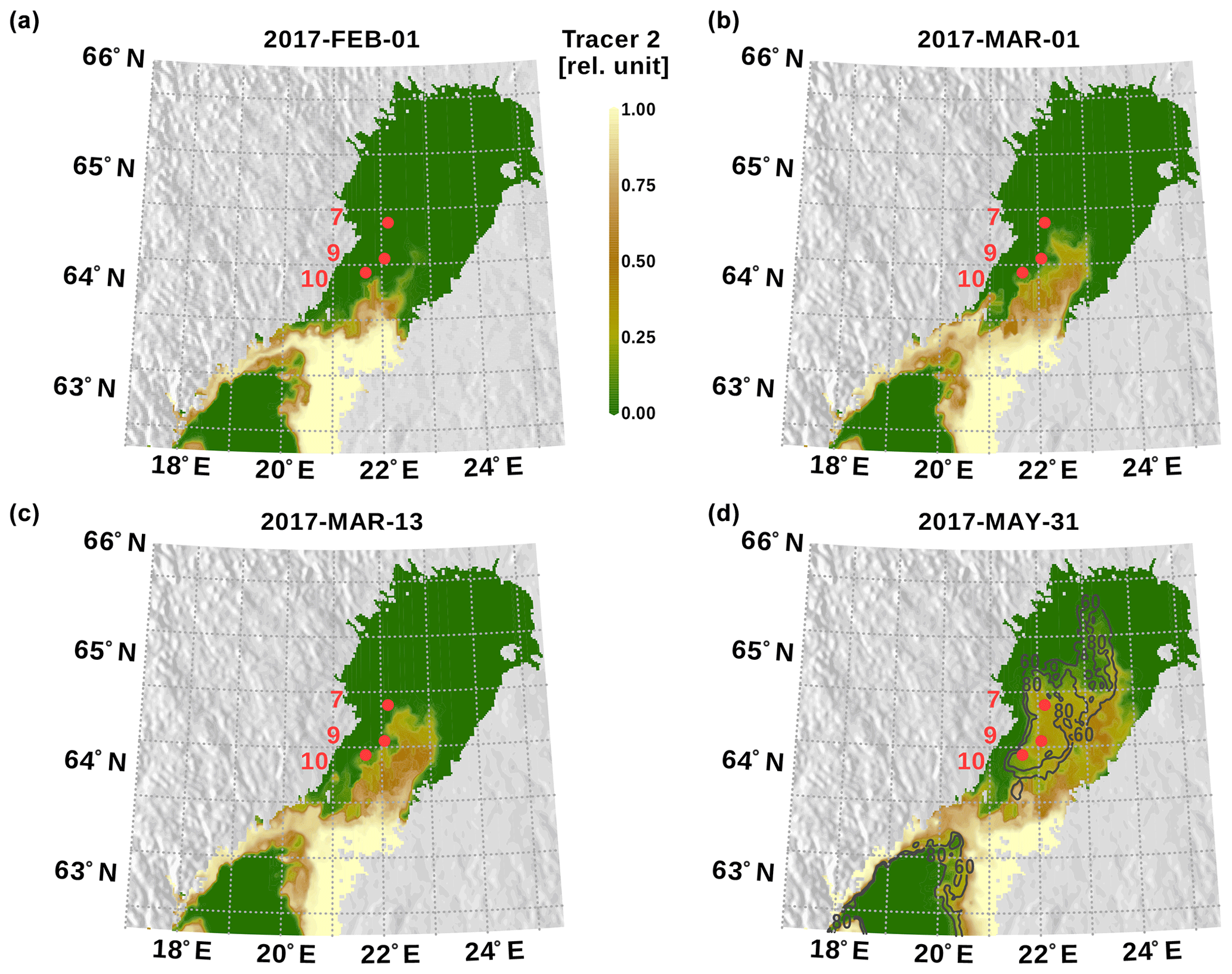
Figure 10Bothnian Sea surface tracer concentration in the bottom model layer. Red dots indicate the observation stations. In panel (d), bathymetry contour lines for 60 and 80 m depths are shown.
The propagation of Bothnian Sea surface tracer is shown in Fig. 10 as the surface tracer concentration just above the sea floor, i.e., former surface water already descended to the bottom. Surface water from the Bothnian Sea arrives at the area of our observations in mid-March. The snapshot from 31 May shows the areas which are ventilated until the end of the model simulation where the dense water plume arrives at the most northern deep parts of the basin.
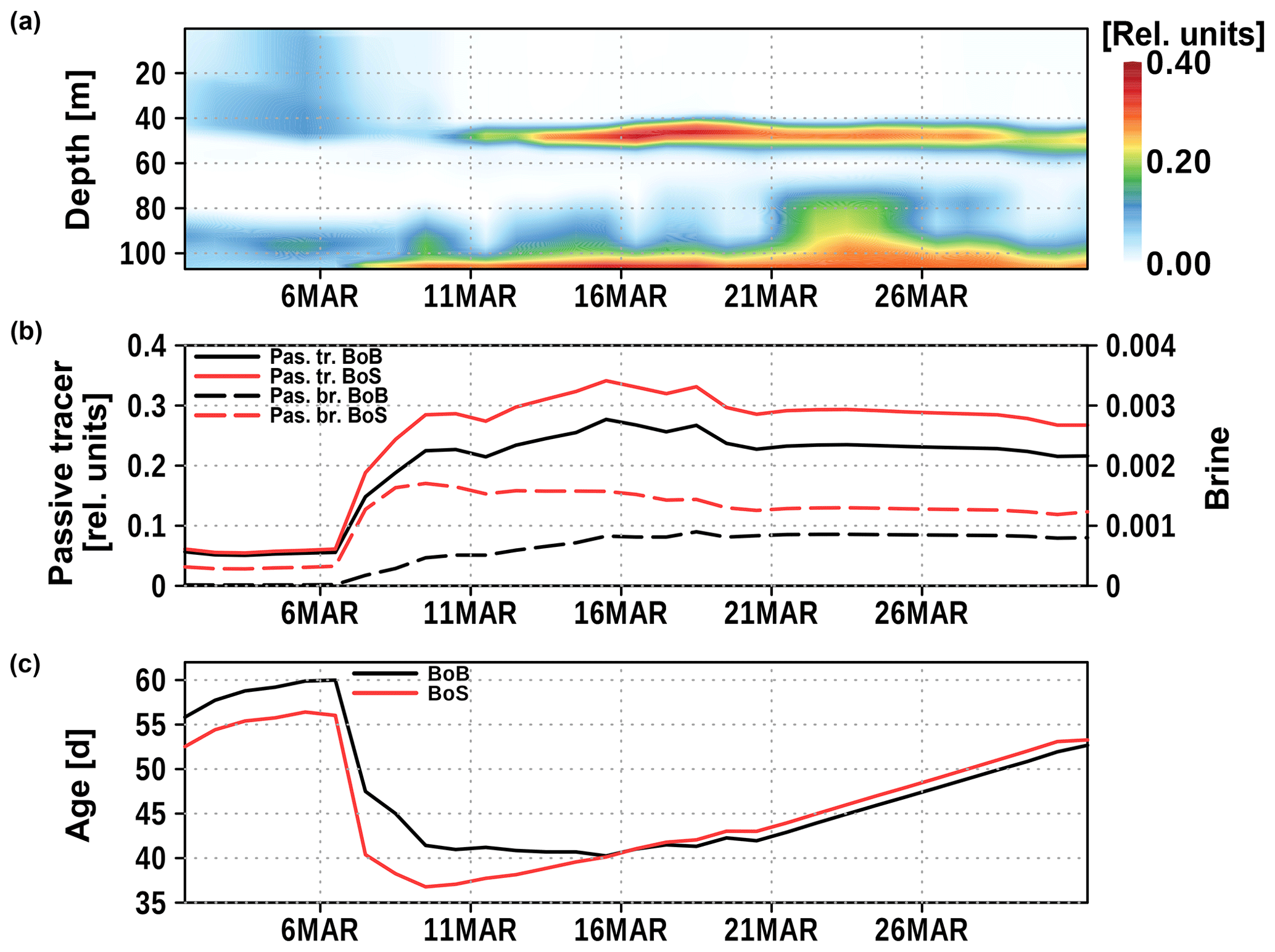
Figure 11Time series of Bothnian Sea and Bay surface tracer at station 9 (Fig. 3). Panel (a) shows the vertical distribution of Bothnian Sea surface water; panel (b) shows the concentrations of Bothnian Sea (red) and Bothnian Bay (black) surface water, and the concentration of brine (dashed, right y axis) in the bottom water at station 9; panel (c) shows the mean age of Bothnian Sea and Bothnian Bay surface water in the bottom water at station 9.
In Fig. 11, we show the time development of the surface tracer concentrations at station 9. A considerable concentration of Bothnian Sea surface water arrives around 10 March in the bottom water of station 9. Both surface tracers, from the Bothnian Bay and the Bothnian Sea, account for 50 %–60 % of the bottom water. The contribution of brine is less than 1 % and negligible. The mean age of surface water is shown in Fig. 11c. In the beginning of March, it shows the age of the small amount of surface water that arrived shortly after the simulation had been started. The mean age decreases by 20–25 d when the pulse of surface water (7–10 March) arrives. The last surface contact of Bothnian Sea water was about 35 d prior, i.e., around 1 February. At this time, surface water masses from the Bothnian Sea and Bothnian Bay have been mixed. The resulting density initiated a downslope transport into the Bothnian Sea from the surface.
In March 2017, a well-oxygenated and cold bottom water layer was observed at station 9 in the center of the Bothnian Bay (Fig. 7). The water column showed a pronounced density stratification mainly due to a halocline in about 80 m depth with less oxygen than in the bottom water. Therefore, it is very likely that the oxygen-rich water arrived at this position rather by lateral intrusion or inflow than by vertical mixing. In the sea-ice-covered Bothnian Bay, two mechanisms potentially could have produced the observed water mass. (i) Bothnian Sea surface water crossed the Northern Quark, was mixed with Bothnian Bay surface water, descended to the bottom due to high density, and followed the topography into the basin, or (ii) brine release from sea ice and ambient water formed a denser water mass, preferentially in shallower coastal areas which then, as a gravity current, arrived at the deep basin.
The low temperature and the very high oxygen concentration (Fig. 7) reveal that the contributing water masses were in contact with the surface recently. A TS analysis in Fig. 8 suggest that mixing of the observed Bothnian Sea (magenta dots) and Bothnian Bay water hardly can result in the observed oxygen-rich and cold bottom water. Only a small portion of Bothnian Bay water in about 40–50 m depth (blue dots) shows the appropriate TS properties. However, assuming temperatures would be higher earlier in the winter season, surface water from the Bothnian Sea and from the Bothnian Bay can mix into the observed bottom water.
The model simulation with a passive tracer approach supports these findings. The majority of new bottom water is formed from surface water which starts to descend in the beginning of February.
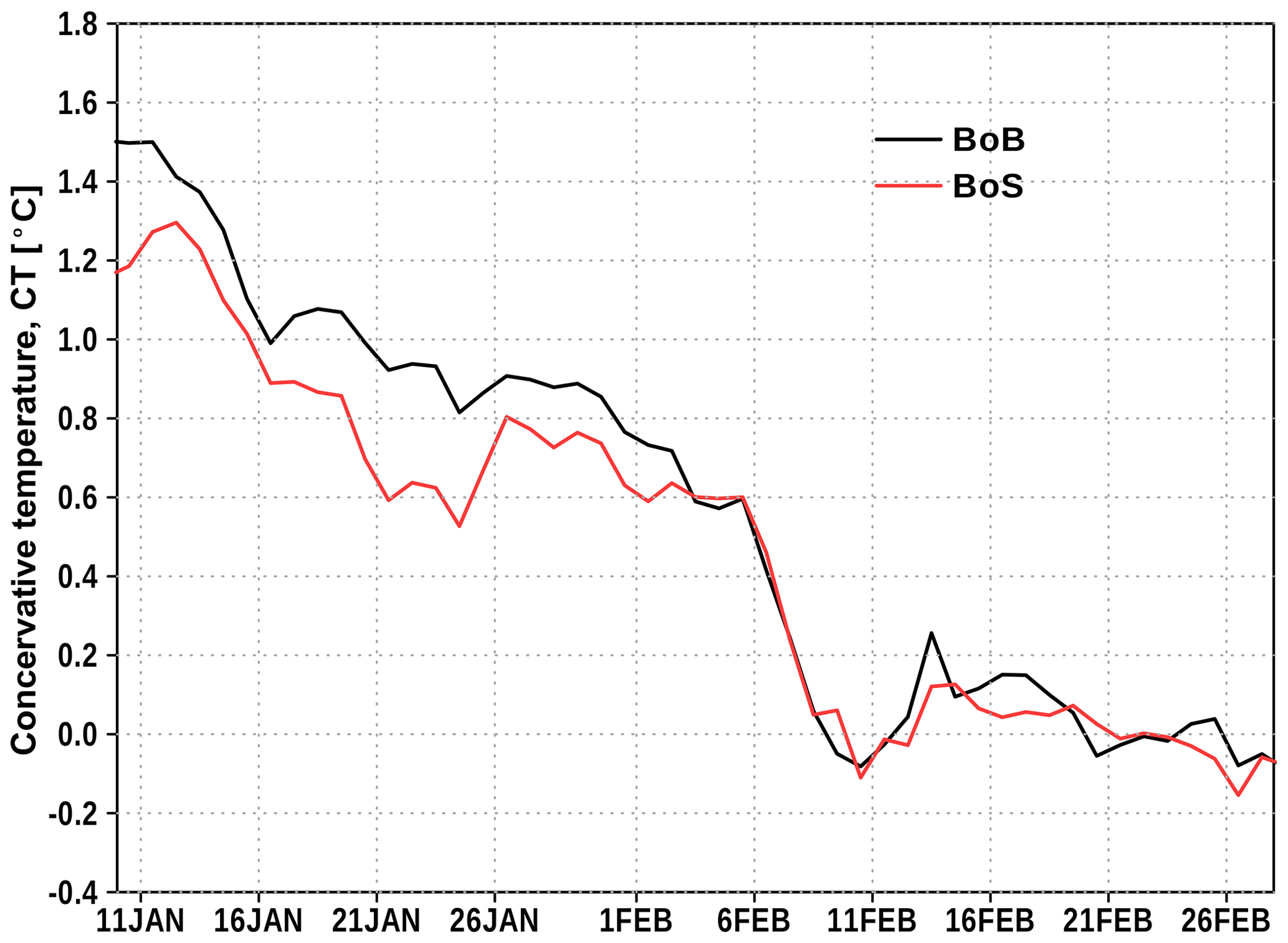
Figure 12Model SST in the southern Bothnian Bay (black) and the northern Bothnian Sea (red).
We show in Fig. 12 the sea surface temperature (SST) development as seen in our model simulation. The shown SST is an area average for the southern Bothnian Bay and the northern Bothnian Sea. In both areas, the SST simultaneously decreases and a suitable SST, forming the observed bottom water, can be found in the beginning of February.
However, approximately 30 % of simulated bottom water was not in contact with the surface. This is also evident from the simulated temperature. It drops from 2.8 to 1.6 ∘C with the arrival of the new water mass and reflects that about one third is from older and warmer, intermediate or bottom water. The overestimation of entrainment is a known issue of z-coordinate models, especially for down flowing dense water plumes (Winton et al., 1998).
Harvey et al. (2015) show a linear relationship between CDOM fluorescence and CDOM absorption, and CDOM absorption and salinity (negative slope) in the Bothnian Sea, resulting in a linear relationship (negative slope) between CDOM fluorescence and salinity. Figure 9 clearly shows this relationship. Assuming that CDOM (yellow substances) are largely conservative, the bottom water at station 9 could be the result of mixing Bothnian Sea and Bothnian Bay water. For an analysis of water masses, we estimate the mixing ratio (mx). The mx is the volume ratio of Bothnian Bay surface water SBS to Bothnian Sea surface water SQ giving Bothnian Bay bottom water SBB based on measured salinity.
With the salinity of the surface water at station 12 SQ=4.9, of Bothnian Bay surface water SBS=3.0, and of Bothnian Bay bottom water at station 9 SBB=3.75, mx is 1.53. Using this mixing ratio, we can estimate the CDOM concentration in the Bothnian Bay bottom water: given surface CDOM concentrations in the Bothnian Sea (15.4 mg m−3) and Bothnian Bay (24 mg m−3) result in a bottom water concentration in the Bothnian Bay of 20.6 mg m−3. This value is close to the observed value of 21 mg m−3 (Fig. 7).
Mixing of brine and Bothnian Bay surface water cannot decrease CDOM to the observed level. If CDOM behaves similarly to salt during freezing, that is, concentration increases in brine, the mixed water would show an elevated CDOM concentration like salt. Müller et al. (2011) and Müller et al. (2013) showed that CDOM is enriched in sea ice compared to salt. The enrichment factor of CDOM in sea ice relative to salt is on the order of 1.3. Therefore, the CDOM concentration in brine is less increased than salinity but still higher than in the surface water and a brine induced bottom water would have higher CDOM concentrations than the surface water. These findings agree with our model simulations showing virtually no brine in the bottom water (Fig. 11).
Model simulations and observations show that bottom water ventilation in the Bothnian Sea is due to mixing of surface water at the Northern Quark forming dense water which then initiates a downflow cascade into the Bothnian Bay. Shapiro et al. (2003) developed a theory for dense water cascades at continental shelves and derived a criterion discriminating between an accelerated event and a steady Ekman layer flow. The conditions for an accelerated cascade (Shapiro et al., 2003, Eq. 9) are not fulfilled in the case of the Bothnian Bay; thus, the downslope flow is rather a bottom boundary layer Ekman flow than an accelerated event.
A density estimate based on our observed data shows that the density gradient between Bothnian Bay bottom water and surface water at the Northern Quark vanishes if the SST exceeds 8 ∘C. Therefore, ventilation will occur in winter only.
During a cruise in March 2017, we took sea ice samples in the northern Baltic Sea, the Bothnian Bay. The bulk ice salinity was about 0.6 g kg−1. Brine samples showed a salinity of about 15 g kg−1 and the surface water a salinity of about 3 g kg−1. In addition, CTD casts were performed at three different locations. At one location, the bottom water was saturated with oxygen and the temperature was very low (0.3 ∘C) compared to the other two stations. We find that this bottom water was formed due to a recent intrusion of former surface water. Complementing the observations, a numerical model experiment has been designed allowing to track different water masses.
Observations, and especially CDOM data, exclude a mechanism where brine contributes to dense water formation. Also the model simulation gives no evidence for a contribution of brine.
The plausible ventilation mechanism is the inflow of Bothnian Sea surface water into the Bothnian Bay. We found a possible time for such an inflow 5 weeks before our measurements. This mechanism can only work if the sea surface salinity of the adjacent basin is considerably higher than the salinity of the bottom water. A prerequisite for this configuration is a shallow sill separating the basins. The depths have to be sufficiently shallower than the halocline to prevent saline deep water inflows. A necessary horizontal density gradient is established only for a low surface water temperature. Consequently, these ventilation events occur in the winter season. These findings confirm Marmefelt and Omstedt (1993), who excluded haline convection for the Bothnian Sea based on budget estimates and considered this process as very unlikely for the Bothnian Bay.
We observed the ventilation at one station only. However, the model simulation shows that the dense water plume progresses further northward during spring and ventilates also the northernmost part. We are aware that our observations are a snapshot supported by numerical model simulations. Therefore, we are planning an extended campaign including moorings equipped with current meters. The model simulations are an excellent tool stimulating and guiding CTD and mooring stations.
All sea ice and brine data are in this text. Data from the hand-held CTD and shipborne CTD data are available from https://doi.org/10.12754/data-2019-0002. Model simulation data are freely available from https://thredds-iow.io-warnemuende.de/thredds/catalogs/publications/thomas/catalog_neumann2020_ref.html?dataset=IOW-THREDDS-Baltic_ref_2020-04-21-10 (Neumann, 2020).
In this section, we demonstrate the model performance for reproducing sea ice, temperature, and salinity in the northern Baltic Sea. Although the model run starts in 1948, we show the validation from 1990 to 2018, the last 30 years of the simulation. We skip the first 40 years, because the model was still drifting due to the long residence time of the Baltic Sea, especially in the northern parts.
Figure A1 shows the annual maximum ice extent from observations (red bars) and from the model simulation (green bars). The variability is well reproduced by the model, while in most years the extent is somewhat overestimated. In the model, we summed up all ice classes including frazil which might not always be part of the observations.
In the following figures, we show temperature and salinity data from two stations in the Bothnian Bay and in the Bothnian Sea, respectively. We focus on surface data (green) and data from close to the sea floor (blue). All observations are freely distributed by ICES (http://www.ices.dk, last access: 19 June 2020). In Fig. A2, the locations of the two stations are shown.
Temperature and salinity are reasonably reproduced in the Bothnian Bay (station F9). A weakness are the low bottom temperature events which are not reproduced well by the model. The reason is the overestimation of entrainment in z-coordinate models as discussed in Sect. 4.
Salinity in the Bothnian Sea (station SR5) bottom water is overestimated by approximately 0.5 g kg−1. Surface salinity and temperature show a reasonably good performance.
In summary, we assess that the model is able to reproduce the relevant processes sufficiently. The experiment with the passive tracers shows that despite the enhanced entrainment also the ventilation of bottom water is reflected in the model.
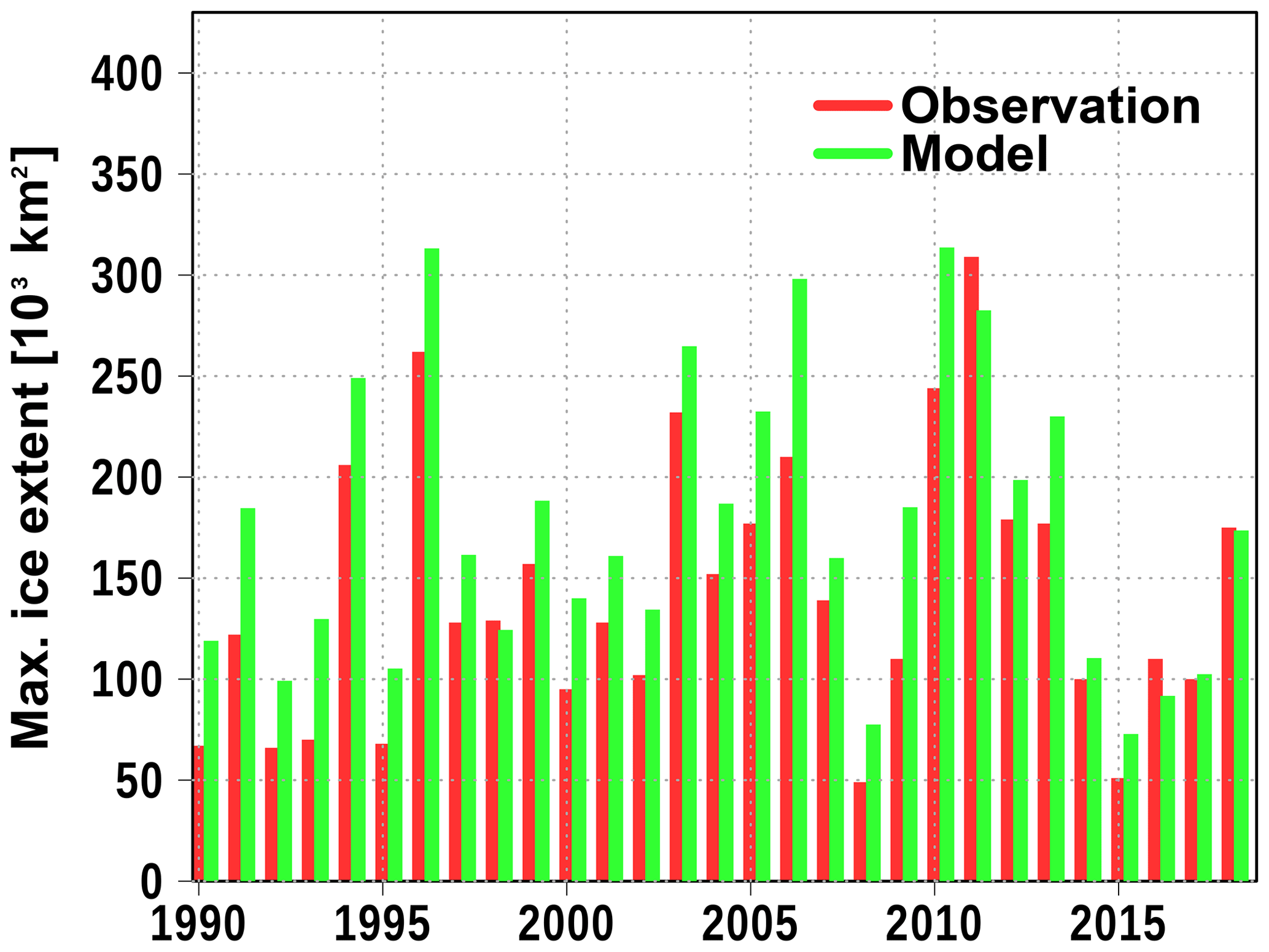
Figure A1Simulated (green) and observed (red) maximum sea ice extent. Observations are obtained freely from https://en.ilmatieteenlaitos.fi/ice-winter-in-the-baltic-sea (last access: 19 June 2020).
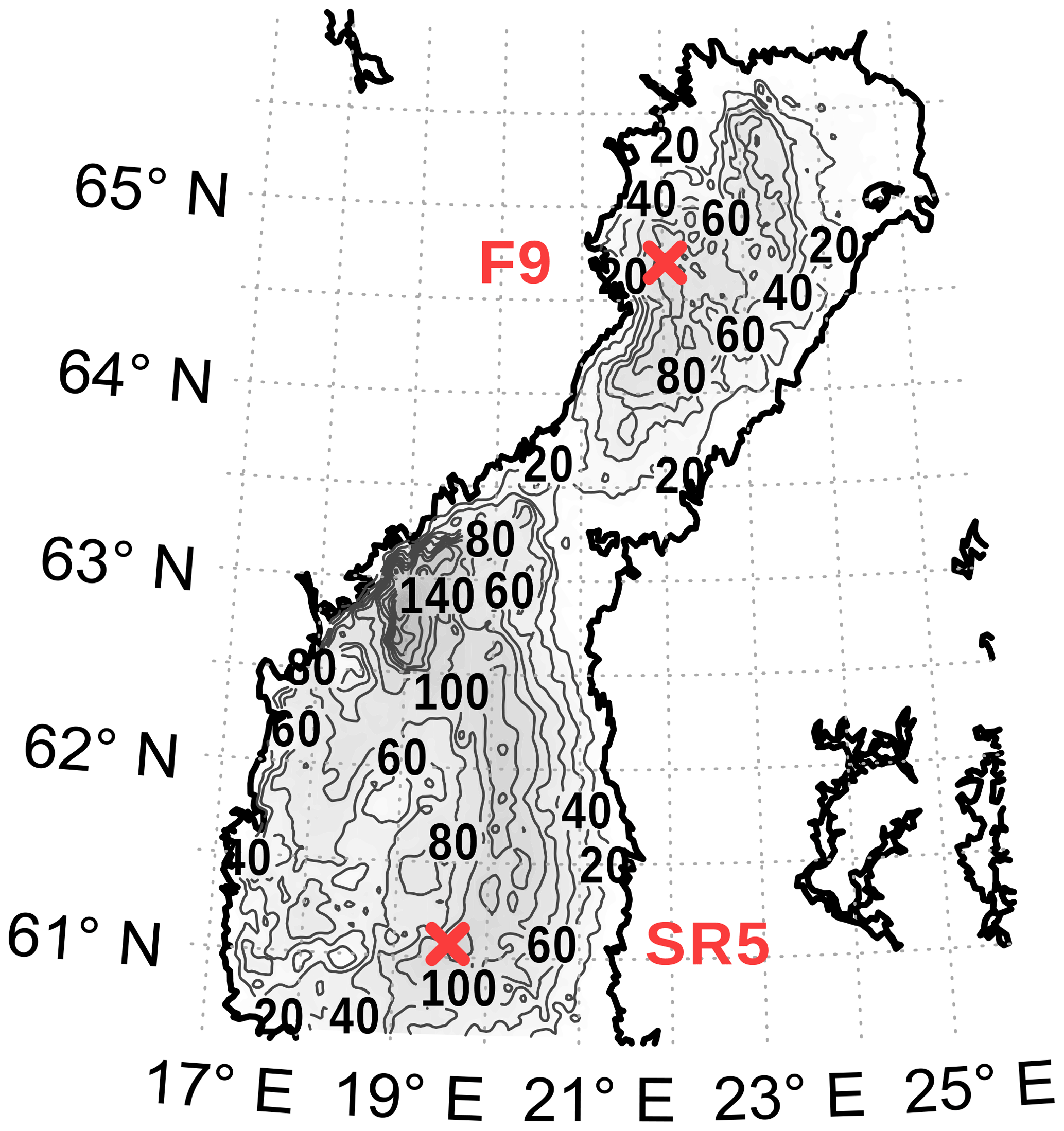
Figure A2Location of the validation stations. The map was created using the software package GrADS 2.1.1.b0 (http://cola.gmu.edu/grads/, last access: 19 June 2020), using published bathymetry data (Seifert et al., 2008).
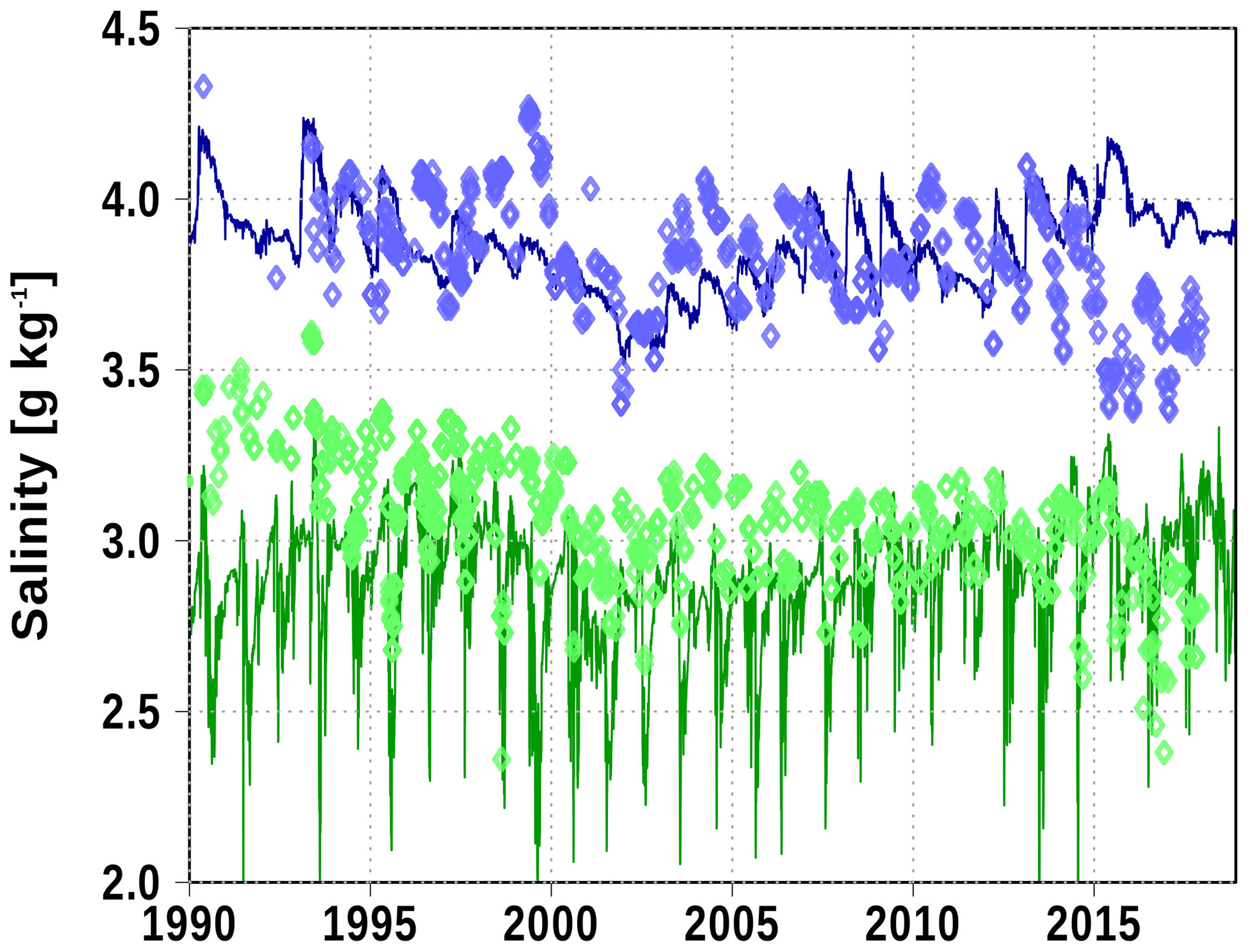
Figure A3Surface (green) and bottom (blue) salinity at station F9. Solid line: model; diamonds: observations (http://www.ices.dk, last access: 19 June 2020).
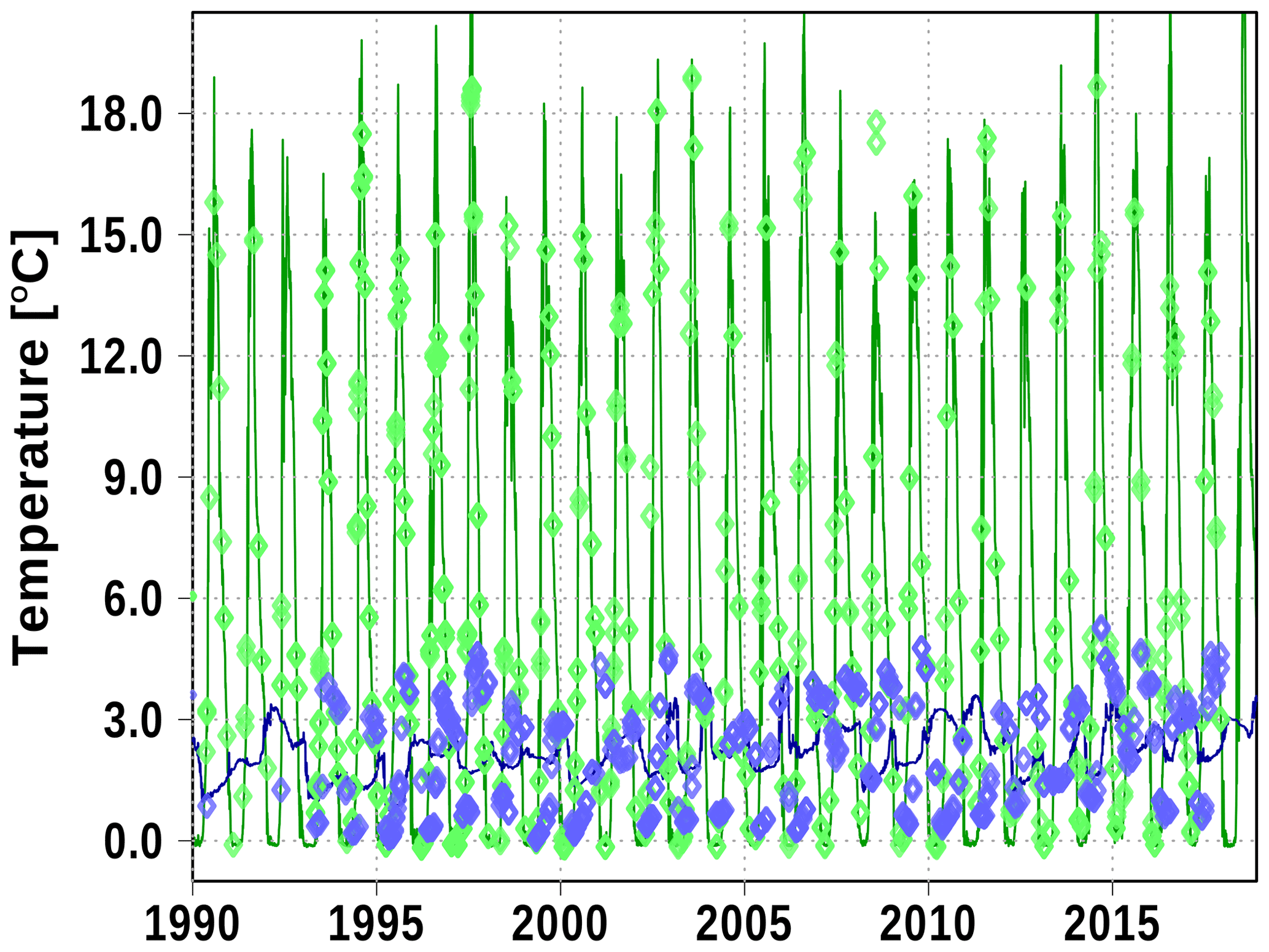
Figure A4Surface (green) and bottom (blue) temperature at station F9. Solid line: model; diamonds: observations (http://www.ices.dk, last access: 19 June 2020).
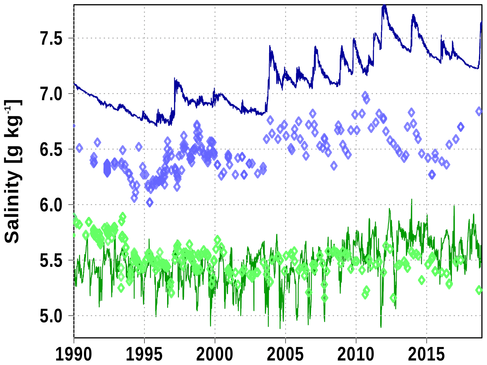
Figure A5Surface (green) and bottom (blue) salinity at station SR5. Solid line: model; diamonds: observations (http://www.ices.dk, last access: 19 June 2020).
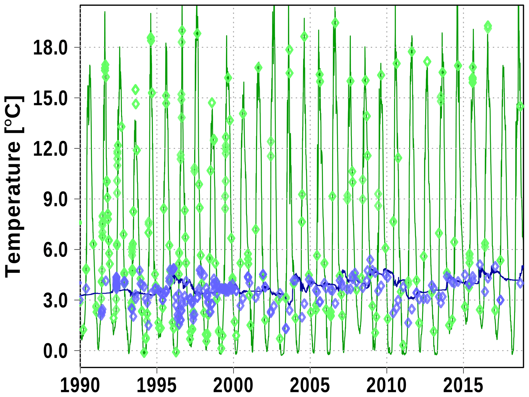
Figure A6Surface (green) and bottom (blue) temperature at station SR5. Solid line: model; diamonds: observations (http://www.ices.dk, last access: 19 June 2020).
TN and MM designed the experiment; TN designed and performed the model simulations; HS and MG performed optical measurements; MK and DH performed CTD and ice core measurements. All authors contributed to data analysis and writing the manuscript.
The authors declare that they have no conflict of interest.
We are very grateful for the assistance of the crew members of the RV Maria S. Merian who made possible research in the sea-ice-covered Baltic Sea. Chief scientist Ralph Schneider always supported our experiments, especially the sea ice coring. Ingo Schuffenhauer operated the CTD and the salinometer. Computational power was provided by the North-German Supercomputing Alliance (HLRN). We are very grateful to three anonymous referees who helped considerably to improve the manuscript.
The publication of this article was funded by the Open Access Fund of the Leibniz Association.
This paper was edited by John M. Huthnance and reviewed by three anonymous referees.
Aagaard, K., Coachman, L., and Carmack, E.: On the halocline of the Arctic Ocean, Deep-Sea Res., 28, 529–545, https://doi.org/10.1016/0198-0149(81)90115-1, 1981. a
Assur, A.: Composition of Sea Ice and its Tensile Strength, in: Arctic Sea Ice, 106–138, U.S. National Academy of Science – National Research Council, Washington, D.C., 1958. a
Baltic Icebreaking Management: Baltic Sea Icebreaking Report 2016–2017, Tech. rep., Baltic Icebreaking Management, available at: http://baltice.org/app/static/pdf/BIM Report 16-17.pdf (last access: 19 June 2020), 2017. a
Geyer, B. and Rockel, B.: coastDat-2 COSMO-CLM Atmospheric Reconstruction, https://doi.org/10.1594/WDCC/coastDat-2_COSMO-CLM, 2013. a
Granskog, M., Kaartokallio, H., Kuosa, H., Thomas, D. N., and Vainio, J.: Sea ice in the Baltic Sea? A review, Estuarine, Coastal and Shelf Science, 70, 145–160, https://doi.org/10.1016/j.ecss.2006.06.001, 2006. a
Granskog, M. A., Kaartokallio, H., Kuosa, H., Thomas, D. N., Ehn, J., and Sonninen, E.: Scales of horizontal patchiness in chlorophyll a, chemical and physical properties of landfast sea ice in the Gulf of Finland (Baltic Sea), Polar Biology, 28, 276–283, https://doi.org/10.1007/s00300-004-0690-5, 2005. a
Griffies, S. M.: Fundamentals of Ocean Climate Models, Princeton University Press, Princeton, NJ, 2004. a
Harvey, E. T., Kratzer, S., and Andersson, A.: Relationships between colored dissolved organic matter and dissolved organic carbon in different coastal gradients of the Baltic Sea, AMBIO, 44, 392–401, https://doi.org/10.1007/s13280-015-0658-4, 2015. a, b
ICO, SCOR, and IAPSO: The international thermodynamic equation of seawater – 2010: Calculation and use of thermodynamic properties., Tech. Rep. 56, Intergovernmental Oceanographic Commission, Manuals and Guides, UNESCO, 2010. a
Ivanov, V., Shapiro, G., Huthnance, J., Aleynik, D., and Golovin, P.: Cascades of dense water around the world ocean, Prog. Oceanogr., 60, 47–98, https://doi.org/10.1016/j.pocean.2003.12.002, 2004. a
Jerlov, N. (Ed.): Marine Optics, vol. 14 of Elsevier Oceanography Series, Elsevier, https://doi.org/10.1016/S0422-9894(08)70789-X, Amsterdam, Oxford, New York, 1976. a
Kabel, K., Moros, M., Porsche, C., Neumann, T., Adolphi, F., Andersen, T. J., Siegel, H., Gerth, M., Leipe, T., Jansen, E., and Sinninghe Damsté, J. S.: Impact of climate change on the Baltic Sea ecosystem over the past 1000 years, Nat. Clim. Change, 2, 871–874, https://doi.org/10.1038/nclimate1595, 2012. a
Kirk, J. T.: Light and Photosynthesis in Aquatic Ecosystems, 2nd edn., Cambridge University Press, New York, 1994. a, b
Lass, H.-U. and Matthäus, W.: General Oceanography of the Baltic Sea, chap. 2, 5–43, Wiley-Blackwell, Hoboken, New Jersey, https://doi.org/10.1002/9780470283134.ch2, 2008. a
Marmefelt, E. and Omstedt, A.: Deep water properties in the Gulf of Bothnia, Cont. Shelf Res., 13, 169–187, https://doi.org/10.1016/0278-4343(93)90104-6, 1993. a, b, c, d
Meiners, K., Fehling, J., Granskog, M. A., and Spindler, M.: Abundance, biomass and composition of biota in Baltic sea ice and underlying water (March 2000), Polar Biol., 25, 761–770, https://doi.org/10.1007/s00300-002-0403-x, 2002. a
Mohrholz, V.: Major Baltic Inflow Statistics – Revised, Front. Mar. Sci., 5, 384, https://doi.org/10.3389/fmars.2018.00384, 2018. a
Moros, M., Kotilainen, A. T., Snowball, I., Neumann, T., Perner, K., Meier, H. M., Leipe, T., Zillén, L., Sinninghe Damsté, J. S., and Schneider, R.: Is deep-water formation in the Baltic Sea a key to understanding seabed dynamics and ventilation changes over the past 7000 years?, Quatern. Int., in press, https://doi.org/10.1016/j.quaint.2020.03.031, 2020. a
Müller, S., Vähätalo, A. V., Granskog, M. A., Autio, R., and Kaartokallio, H.: Behaviour of dissolved organic matter during formation of natural and artificially grown Baltic Sea ice, Ann. Glaciol., 52, 233–241, https://doi.org/10.3189/172756411795931886, 2011. a, b
Müller, S., Vähätalo, A. V., Stedmon, C. A., Granskog, M. A., Norman, L., Aslam, S. N., Underwood, G. J., Dieckmann, G. S., and Thomas, D. N.: Selective incorporation of dissolved organic matter (DOM) during sea ice formation, Mar. Chem., 155, 148–157, https://doi.org/10.1016/j.marchem.2013.06.008, 2013. a, b
Neumann, T.: Climate-change effects on the Baltic Sea ecosystem: A model study, J. Mar. Sys., 81, 213–224, https://doi.org/10.1016/j.jmarsys.2009.12.001, 2010. a
Neumann, T.: Tracer Experiment Bothnian Bay, available at: https://thredds-iow.io-warnemuende.de/thredds/catalogs/publications/thomas/catalog_neumann2020_ref.html?dataset=IOW-THREDDS-Baltic_ref_2020-04-21-10, last access: 29 June 2020. a
Neumann, T., Siegel, H., and Gerth, M.: A new radiation model for Baltic Sea ecosystem modelling, J. Mar. Sys., 152, 83–91, https://doi.org/10.1016/j.jmarsys.2015.08.001, 2015. a
Nguyen, A. T., Menemenlis, D., and Kwok, R.: Improved modeling of the Arctic halocline with a subgrid-scale brine rejection parameterization, J. Geophys. Res.-Oceans, 114, C11014, https://doi.org/10.1029/2008JC005121, 2009. a, b
Peterson, A. K.: Observations of brine plumes below melting Arctic sea ice, Ocean Sci., 14, 127–138, https://doi.org/10.5194/os-14-127-2018, 2018. a
Raateoja, M.: Deep-water oxygen conditions in the Bothnian Sea, Boreal Env. Res., 18, 235–249, 2013. a
Seifert, T., Tauber, F., and Kayser, B.: Digital topography of the Baltic Sea, available at: https://www.io-warnemuende.de/topography-of-the-baltic-sea.html (last access: 15 July 2019), 2008. a, b, c
Shapiro, G. I., Huthnance, J. M., and Ivanov, V. V.: Dense water cascading off the continental shelf, J. Geophys. Res.-Oceans, 108, 3390, https://doi.org/10.1029/2002JC001610, 2003. a, b, c
Skogseth, R., Smedsrud, L. H., Nilsen, F., and Fer, I.: Observations of hydrography and downflow of brine-enriched shelf water in the Storfjorden polynya, Svalbard, J. Geophys. Res.-Oceans, 113, C08049, https://doi.org/10.1029/2007JC004452, 2008. a
Stigebrandt, A.: A Model for the Vertical Circulation of the Baltic Deep Water, J. Phys. Oceanogr., 17, 1772–1785, https://doi.org/10.1175/1520-0485(1987)017<1772:AMFTVC>2.0.CO;2, 1987. a, b
Winton, M.: A Reformulated Three-Layer Sea Ice Model, J. Atmos. Ocean. Technol., 17, 525–531, https://doi.org/10.1175/1520-0426(2000)017<0525:ARTLSI>2.0.CO;2, 2000. a
Winton, M., Hallberg, R., and Gnanadesikan, A.: Simulation of Density-Driven Frictional Downslope Flow in Z-Coordinate Ocean Models, J. Phys. Oceanogr., 28, 2163–2174, https://doi.org/10.1175/1520-0485(1998)028<2163:SODDFD>2.0.CO;2, 1998. a
The requested paper has a corresponding corrigendum published. Please read the corrigendum first before downloading the article.
- Article
(13870 KB) - Full-text XML