the Creative Commons Attribution 4.0 License.
the Creative Commons Attribution 4.0 License.
 | 15 Jun 2020
Mechanisms of decadal changes in sea surface height and heat content in the eastern Nordic Seas
Sara Broomé
Léon Chafik
Johan Nilsson
The Nordic Seas constitute the main ocean conveyor of heat between the North Atlantic Ocean and the Arctic Ocean. Although the decadal variability in the subpolar North Atlantic has been given significant attention lately, especially regarding the cooling trend since the mid-2000s, less is known about the potential connection downstream in the northern basins. Using sea surface heights from satellite altimetry over the past 25 years (1993–2017), we find significant variability on multiyear to decadal timescales in the Nordic Seas. In particular, the regional trends in sea surface height show signs of a weakening since the mid-2000s, as compared to the rapid increase in the preceding decade since the early 1990s. This change is most prominent in the Atlantic origin waters in the eastern Nordic Seas and is closely linked, as estimated from hydrography, to heat content. Furthermore, we formulate a simple heat budget for the eastern Nordic Seas to discuss the relative importance of local and remote sources of variability; advection of temperature anomalies in the Atlantic inflow is found to be the main mechanism. A conceptual model of ocean heat convergence, with only upstream temperature measurements at the inflow to the Nordic Seas as input, is able to reproduce key aspects of the decadal variability in the heat content of the Nordic Seas. Based on these results, we argue that there is a strong connection with the upstream subpolar North Atlantic. However, although the shift in trends in the mid-2000s is coincident in the Nordic Seas and the subpolar North Atlantic, the eastern Nordic Seas have not seen a reversal of trends but instead maintain elevated sea surface heights and heat content in the recent decade considered here.
- Article
(7797 KB) - Full-text XML
- BibTeX
- EndNote


The Nordic Seas, a collective name for the Greenland–Iceland–Norwegian seas, are the link between the Atlantic and the Arctic oceans and are recognized to play an important role in the global climate system (Drange et al., 2005). Warm and saline waters of Atlantic origin cross the Greenland–Scotland Ridge (Fig. 1) and flow northward through the eastern part of the Nordic Seas before entering into the Arctic Ocean (Mauritzen, 1996; Orvik and Niiler, 2002; Skagseth et al., 2008; Furevik et al., 2007), affecting the local sea ice and atmosphere on its way. The densest waters sustaining the lower limb of the Atlantic Meridional Overturning Circulation (Chafik and Rossby, 2019) are also produced in this region, by heat loss to the atmosphere, before flowing southward at depth across the Greenland–Scotland Ridge into the North Atlantic Ocean (Mauritzen, 1996; Hansen and Østerhus, 2000).
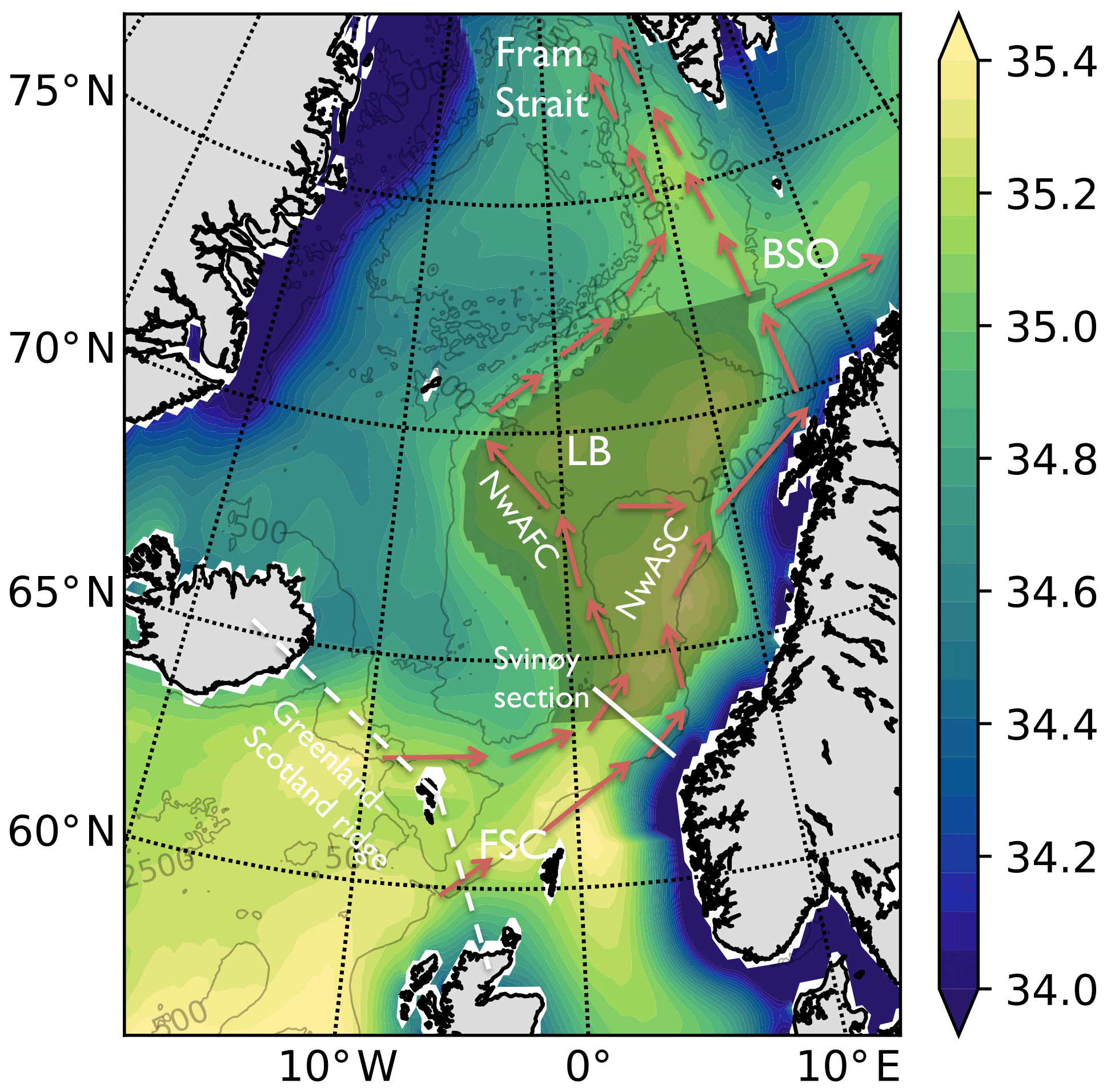
Figure 1Map of the Nordic Seas with average surface salinity (Zweng et al., 2013) in shading. The general pathways of the Norwegian Atlantic Front Current (NwAFC) and the Norwegian Atlantic Slope Current (NwASC) are indicated together with the Lofoten Basin (LB), Barents Sea Opening (BSO), Fram Strait, parts of the Greenland–Scotland Ridge, the Faroe–Shetland Channel (FSC) and the Svinøy hydrographic section. The darker shaded region is the area enclosed by the mean location of the 35.0 surface salinity isohaline between 63.5 and 72.5∘ N. This area represents the Atlantic water (AW) area in the current study. Grey contours are bathymetry (Becker et al., 2009).
Since the Nordic Seas make up a major source of heat for the Arctic Ocean it is important to understand the thermal variability and the mechanisms behind it. The Nordic Seas experience intrinsic variability on many timescales (e.g. Siegismund et al., 2007; Mork et al., 2014; Glessmer et al., 2014; Eldevik et al., 2009; Årthun et al., 2017; Shi et al., 2017). Carton et al. (2011) found several warm and cold events on multiyear timescales in an extensive 60-year hydrographic record. Segtnan et al. (2011) used reanalysis to examine the heat and freshwater budgets and find the largest water mass modifications to occur in the eastern part of the Nordic Seas. Asbjørnsen et al. (2018) used a consistent model framework to set up a closed heat and freshwater budget. A common question that these studies and many others address is if the source of variability is local, by interaction with the atmosphere, or remote and advected into the Nordic Seas. Anomalies have been found to propagate from the North Atlantic over the Greenland–Scotland Ridge (Årthun and Eldevik, 2016; Furevik, 2000; Koszalka et al., 2013), and the Atlantic inflow is tightly linked to dynamics of the subpolar gyre (Hátún et al., 2005). Interestingly, the subpolar North Atlantic has recently experienced strong decadal variability (Robson et al., 2016; Piecuch et al., 2017; Ruiz-Barradas et al., 2018), but the possible impacts of this further north are not well established. The focus of this study is on recent decadal variability in the Atlantic water domain in the eastern parts of the Nordic Seas, with emphasis on the mechanisms behind the variability.
For a couple of decades now, we have been able to monitor sea level change and study key aspects of ocean dynamics using satellite altimetry. The dynamic sea surface height (SSH) retrieved from satellites carries information on ocean circulation, as it represents streamlines of the surface geostrophic currents, as well as sea level. The SSH reflects both steric height and dynamic bottom pressure (Broomé and Nilsson, 2016); regional sea level change can be related to not only warming/cooling and freshening/salinification by air–sea fluxes but also redistribution of mass, heat and freshwater by time-varying ocean currents (Gill and Niller, 1973; Stammer et al., 2013). On timescales from days to months, local wind forcing and rapidly propagating waves are the main drivers of variability in sea level (Stammer, 1997). On longer timescales, multiyear/interannual-to-decadal, which are relevant to this study, the steric component of the SSH due to the integrated buoyancy of the water column instead becomes the main driver of the variability in sea level (Richter and Maus, 2011). The time series of satellite altimetry starts in 1993 and is now becoming useful for studying recent decadal variability (Chafik et al., 2019).
This study aims to analyse the decadal variability in the Nordic Seas, using the altimetric time series of dynamic SSH combined with in situ data. More specifically, in Sect. 3.1 we find that in addition to a general positive trend in sea level, the Nordic Seas have had a period of rapid increase in SSH followed by a period of slowly increasing SSH. This decadal variability is concentrated in the eastern, Atlantic origin waters. We show that the decadal variability in SSH is linked to heat content, and through a heat budget and conceptual model in Sect. 3.2 we argue that the variation in temperature of the inflowing Atlantic water in the south is the main contributor to the variability. A strong connection to recent decadal variability in the subpolar gyre, discussed in Sect. 3.3, further strengthens this idea, but it also raises some questions about possible variations in the connection over time.
2.1 Satellite altimetry (SSH)
This study has been conducted using satellite altimetry retrieved from E.U. Copernicus Marine Service Information. We use absolute dynamic topography (ADT), which is the sea surface height above the geoid, i.e. the part of the SSH related to the ocean circulation. The gradient of the ADT is directly proportional to the surface geostrophic current. The ADT has undergone several correction, calibration and homogenization processes, bringing data from several satellite missions together (Pujol et al., 2016). The ADT is distributed as daily fields on a regular 1∕4∘ grid and has here been averaged into monthly fields from 1993 until 2017. The monthly time series has been deseasonalized by subtracting a monthly climatology constructed from 1993 to 2017.
2.2 Hydrography
We use the EN4.2.0 data set provided by the UK Met Office (Good et al., 2013), with bias correction by Gouretski and Reseghetti (2010), on a 1∘ horizontal grid and 42 depth levels with higher resolution closer to the surface. Similarly to the ADT, we construct time series of deseasonalized monthly means.
From the hydrographic data, the steric height (ηS) and a baroclinic volume transport function (ψ), proportional to the potential energy anomaly, can be calculated (Gill and Niller, 1973; Walin et al., 2004) as follows:
where
is a nondimensional density anomaly that measures the density deficit of the Atlantic Water (AW) layer relative to the deep water, g is the acceleration of gravity and f is the Coriolis parameter. Note that the steric height is not uniquely defined as it is specified relative to a reference density. However, changes in steric height and in ψ are independent of the reference density. We can decompose the ADT (say η) as (Gill and Niller, 1973)
where and gρηB is a bottom pressure (that again depends on the reference density). Still, ADT and steric height data allow changes in sea level to be partitioned into changes due to steric height and bottom pressure.
The transport stream function ψ is the potential energy anomaly divided by f and represents the vertically integrated thermal-wind flow from to the surface. Note that in a 1.5-layer model with an active upper layer with the depth H, the steric height and baroclinic transport (or potential energy) are closely related and given by (Nilsson et al., 2005)
To capture the dynamics and heat content of the waters of Atlantic origin that occupy the eastern Nordic Seas, integrations are done down to a depth level representative for the time-mean depth of the AW, in this case the EN4 depth level 657 m (see e.g. Skagseth and Mork, 2012). The deep water below the AW is colder and the thermal expansion coefficient lower; thus the contribution to the steric height is supposedly lower. By limiting the integration to 657 m, we exclude the contribution from the deep water that does not experience the same variability as the AW and is not directly affected by the North Atlantic. The depth of the AW is, however, uniform in neither space nor time but extends for example deeper in the Lofoten Basin than it does further south. The analysis is not sensitive to the choice of integration depth, and quantitatively similar spatial patterns and decadal variability are also obtained for integrations extending down to about 1000 m.
2.3 Air–sea heat flux
The net air–sea heat flux has been calculated from five different sources of surface fluxes. Three are from atmospheric reanalyses, ERA-Interim (Dee et al., 2011), NCEP (Kalnay et al., 1996) and JRA-55 (Kobayashi et al., 2015). The National Oceanography Centre (NOC) surface flux (Berry and Kent, 2009, 2011) is calculated from observations of bulk atmospheric properties, and J-OFURO (Tomita et al., 2019) is satellite-derived. Here we have used monthly time series from 1993 to 2013, defined positive upwards, i.e. positive when the ocean loses heat to the atmosphere. All products have been regridded to a grid using bilinear interpolation.
3.1 Sea surface height trends and heat content
Over the last 3 decades, the sea surface height in the Nordic Seas has generally been rising. Figure 2 shows the linear trend in SSH from 1993 to 2017, which is positive almost everywhere and has a local maximum in the AW in the Lofoten Basin of over 0.5 cm yr−1. In parallel, hydrographic observations show that the steric height and the baroclinic transport function (Eqs. 1, 2) have increased during the same period; in Fig. 2 there is also the trend in steric height and transport function, or equivalently potential energy anomaly. Most of the hydrographic trend is in the Atlantic origin sector of the Nordic Seas, and the local maximum is, similarly to the SSH, located in the Lofoten Basin. The heat content of the AW has also increased, and a maximum can again be identified in the Lofoten Basin (Skagseth and Mork, 2012; Mork et al., 2014; Shi et al., 2017). The trends in SSH, steric height (ηS) and baroclinic volume transport (ψ) differ in the shallow shelf regions, but the broad features in areas within the AW that are deeper than 500 m are similar. The pattern of these trends resembles that of the time-mean steric height, and in turn, as the buoyancy of the AW is essentially uniform, the time-mean steric height roughly maps the depth of the AW layer (see Broomé and Nilsson, 2016, Fig. 3). What this reasoning suggests is that the trend in SSH is to a first approximation caused by a uniform warming of the AW. This notion is also supported by Skagseth and Mork (2012).
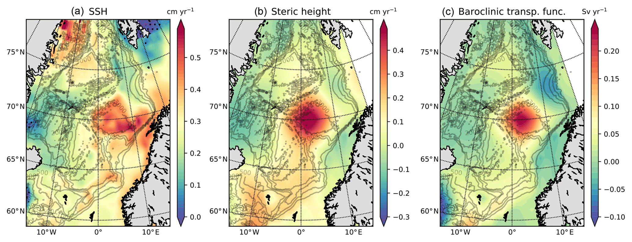
Figure 2(a) Linear trend in SSH (cm yr−1) over the full altimetry period 1993–2017. (b) Linear trend in steric height (cm yr−1) (see Eq. 1) from 1993 to 2016. (c) Linear trend in baroclinic transport function (Sv yr−1; Sv (sverdrup): 106 m3 s−1) (see Eq. 2) from 1993 to 2016. Grey contours are bathymetry (Becker et al., 2009).
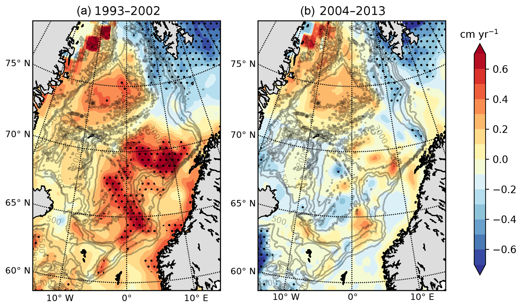
Figure 3Linear trend in SSH (cm yr−1) for (a) 1993–2002 and (b) 2004–2013. A global trend for the full altimetry period 1993–2017 has been removed from the data. Dotted areas are significant at a 95 % confidence level, determined using the two-sided hypothesis Wald test with t distribution (Oliphant, 2007). Grey contours are bathymetry (Becker et al., 2009).
The pattern seen in the trends of the SSH, steric height and potential energy resemble the pattern of the time-mean steric height, more so than that of the time-mean SSH (see e.g. Broomé and Nilsson, 2016, Fig. 3). This indicates that the general warming of the AW during the period 1993 to 2017 also has entailed a gradual reorganization of the circulation both at the surface and over the depth of the AW. The circulation in the AW domain consists of a current system of two branches (Orvik and Niiler, 2002): the Norwegian Atlantic Front Current (NwAFC) and the Norwegian Atlantic Slope Current (NwASC); see Fig. 1. Figure 2 reveals a strengthening of an anticyclonic flow anomaly in the Lofoten Basin, which tends to divert water southeast of the Lofoten Basin (LB) towards the outer NwAFC branch, flowing along the western limit of the LB. Thus, near the LB the trends in AW density serve to strengthen the outer NwAFC branch at the expense of the inner NwASC branch. This is expected to augment the heat transport by the mean flow that enters the LB from the south (Dugstad et al., 2019). Potentially, this could also increase the residence time of the AW in the region as an increasing fraction of the AW tends to follow the NwAFC, taking a longer path along the western edge of the LB. Periods with long-term trends of AW cooling and densification can be expected to show similar patterns of trends in SSH and baroclinic flow as seen in Fig. 2 but with the reversed sign.
The broad-scale positive trend in heat content, steric height and baroclinic transport function in the Lofoten Basin, recorded in the time- and space-interpolated hydrographic data, may partly reflect an increase in the intensity and number of mesoscale anticyclonic eddies shed from the continental slope that propagate into the central basin (Köhl, 2007; Raj et al., 2015; Chafik et al., 2015). Higher influx of eddies from the slope can invigorate the long-lived dominating anticyclonic eddy (Köhl, 2007), known as the Lofoten Vortex, which has a strong local hydrographic signature and moves around in the central basin (Søiland et al., 2016). The associated changes in steric height (Fig. 2) in the Lofoten Basin have served to induce an anticyclonic flow anomaly carrying a larger fraction of AW from the slope current into the basin. This flow anomaly acts to enhance the near-surface heat transport by the mean flow entering the Lofoten Basin from the south (Dugstad et al., 2019). In combination with alterations of eddy fluxes from the Lofoten Escarpment (Spall, 2010; Chafik et al., 2015) the anticyclonic mean-flow anomaly is a plausible mechanism for the build-up of the Lofoten Basin heat content over the period 1993–2017. However, for the large-scale trend pattern it does not matter if the warming in the Lofoten Basin is caused by mesoscale eddies or by mean-flow changes.
Decadal variability
Analysis of the time series of satellite altimetry reveals that the positive trend is not constant in time. Figure 3 shows the linear trend in SSH for two decadal periods, one from 1993 to 2002 and the other from 2004 to 2013. These two periods have very different patterns; the first period has a pronounced positive trend in the AW and also in the Greenland Sea, while the second period has smaller amplitudes and no clear sign of a trend in the AW. It is clear that most of the linear increase seen in Fig. 2 occurs in the first of these periods.
It is also apparent that the greatest change in trend between the two decadal periods occurs in the Atlantic water domain south of the Barents Sea Opening (BSO). To identify the Atlantic water variability we define the AW area, shaded grey in Fig. 1, as the area between 63.5 and 72.5∘ N that is enclosed by the time-mean position of the 35.0 surface isohaline. The defined area comprises the AW from the southern section where different inflows over the Greenland–Scotland Ridge merge into the eastern boundary current system up to and including the deep pool of AW in the Lofoten Basin. North of this, the AW fractionates between the Barents Sea and the continental slope towards the Fram Strait.
The SSH is averaged over the defined AW area, resulting in the time series shown in Fig. 4. The data have been deseasonalized to remove the otherwise-dominant seasonal cycle of high SSH in summer and low SSH in winter, reflecting the seasonal variation in heat content and wind forcing. A large monthly variability remains in addition to a long-term trend of about 0.3 cm yr−1. Around 2004 or 2005, the area-averaged SSH shifts from a period of high variability and positive trend to a stagnant period of smaller variability and no trend.
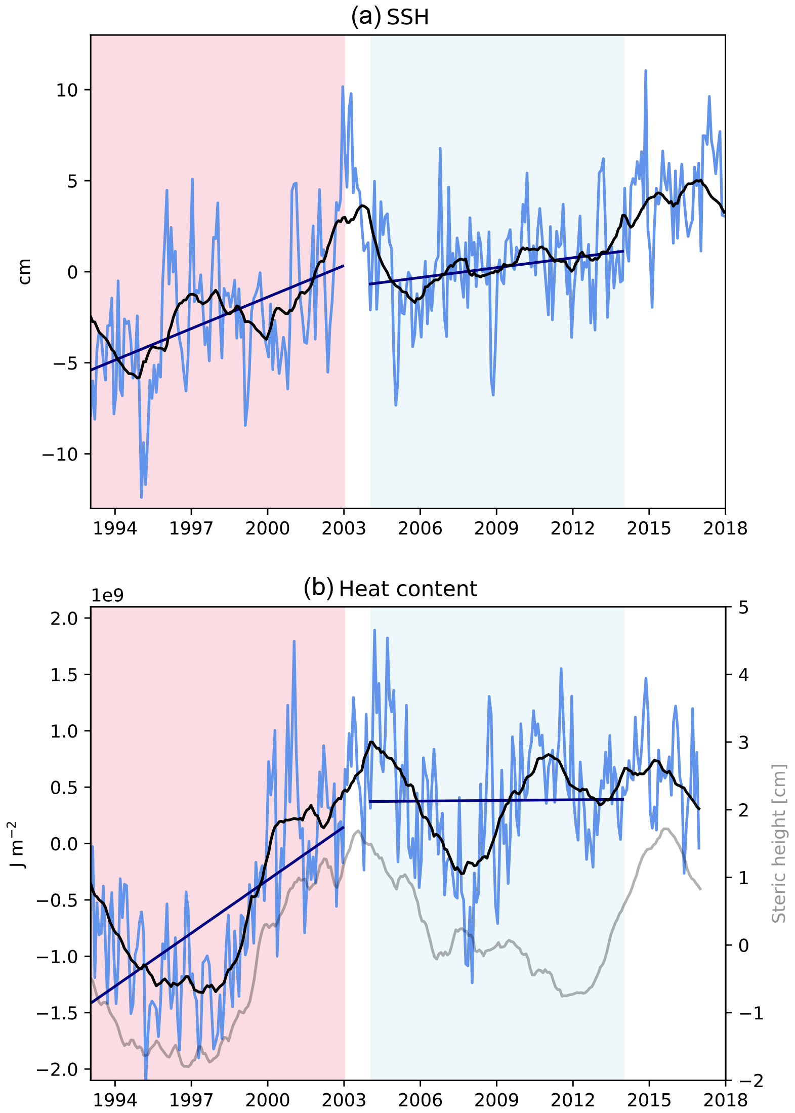
Figure 4(a) Monthly (light blue) and 24-month low-pass-filtered (black) SSH (cm) from 1993 to 2017 averaged over the AW area (see Fig. 1). The SSH has been deseasonalized. In dark blue are the linear trends of the SSH for the two periods 1993–2002 and 2004–2013. (b) Monthly (light blue) and 24-month low-pass-filtered (black) heat content in the upper 657 m of the AW area (J m−2) from 1993 to 2016. The heat content has been deseasonalized. In dark blue are the linear trends for the two periods 1993–2002 and 2004–2013. In grey is the deseasonalized, 24-month low-pass-filtered steric height (cm).
The variations in the SSH on multiyear and longer timescales are closely related to heat content (Richter and Maus, 2011; Shi et al., 2017), and Fig. 4 shows a corresponding AW time series of heat content. The variability on decadal timescales is similar to the SSH; in Fig. 4 there seems to first be a period of strong positive trend of about 5 W m−2, followed by a stagnant period, with the shift in the mid-2000s. This indicates that the observed decadal variability in the SSH is mainly a steric signal, a conclusion made also by Shi et al. (2017), but with some contribution from changes in wind forcing (Chafik et al., 2019). This is further supported by the low-frequency variation in the steric height, shown in grey in Fig. 4b, which closely follows that of the heat content. The exception is around 2010–2011, when the steric height decreased, while the heat content kept increasing, in connection with a strong increase in salinity as seen for example in Fig. 3 in Mork et al. (2019).
The selection of the two periods is somewhat arbitrary, and the trends are generally sensitive to the endpoints. Therefore, the periods should only be considered as guidelines, and the full time series is included for transparency. Here, the altimetric time series has been the basis for the choice. There is an anomalous high event in the SSH around 2003 in Fig. 4, which is well correlated with a deepening of the AW layer, mostly in the Lofoten Basin, and less well correlated with temperature or heat content (Skagseth and Mork, 2012). We have therefore chosen to exclude the year 2003 from the periods.
In the next sections we will discuss the mechanisms behind the changes in trends between the two decadal periods. First, a heat budget will be set up to discern the relative influence of ocean advection and air–sea heat fluxes. Second, based on the heat budget, we will discuss a simple conceptual model to show that changes in the temperature of the Atlantic origin inflow is a likely source of decadal variability. Third, we will analyse the connection between the AW in the Nordic Seas and the upstream subpolar North Atlantic.
3.2 Simple heat budget
A simple heat budget might give insight into the causes of the decadal variability. We consider the heat budget for a fixed volume of Atlantic Water in the Nordic Seas (VAW), defined by the lateral boundaries in Fig. 1 and down to a fixed depth representative of the depth of the AW. The heat content is defined by
where cp is the heat capacity per unit volume for seawater and T is the temperature, and the heat budget is
Here, C is the ocean heat convergence, and Q is the upward net heat flux at the sea surface.
Let us now use the heat budget to examine the heat content for the two decadal periods of interest here, called 1 (first) and 2 (second). Subtracting the budget in Eq. (8) for each period, we can write
where are the averages over periods 1 and 2, respectively, and A is the surface area of the AW domain. The heat content of the AW volume (Fig. 4) has a linear increase during the first period per unit area of about 5 and one of about 0 W m−2 during the second period, i.e.
To analyse if the surface heat flux Q can explain the observed decadal variability, we use observations of net air–sea heat flux. However, the available estimates of surface heat flux differ significantly in pattern, variability and mean state (see e.g. Carton et al., 2018). To demonstrate this, we use five different estimates of the net flux, defined positive upwards, averaged over the two periods of interest and over the AW area; see Table 1 and Fig. 5. In an annual mean, the whole AW area loses heat to the atmosphere, but the mean heat loss in Table 1 varies by about 20 W m−2, or 25 %–30 %, between the products. To explain the observed variability, assuming in turn that the ocean heat divergence is zero, the second decade would have to experience a higher heat loss to the atmosphere, i.e. . This is true for one of the surface flux products (NOC), while the other estimates are close to zero or almost 10 W m−2 in the other direction. The spatial patterns of the difference in surface heat flux between the two periods (Fig. 5) also vary significantly between the data sets, and none of these patterns match the SSH trend pattern (Fig. 2) with its distinct peak in the Lofoten Basin.
Table 1Net surface heat flux Q (W m−2), defined positive upwards, averaged over the AW area (defined in Fig. 1) for the first period 1993–2002 () and the second period 2004–2013 (). The AW area loses heat to the atmosphere in an annual mean. Five different products of surface heat flux are used, as follows: ERA-Interim (reanalysis), JRA-55 (reanalysis), NCEP/NCAR (reanalysis), NOC (in situ observations) and J-OFURO3 (satellite observations). See also Fig. 5.
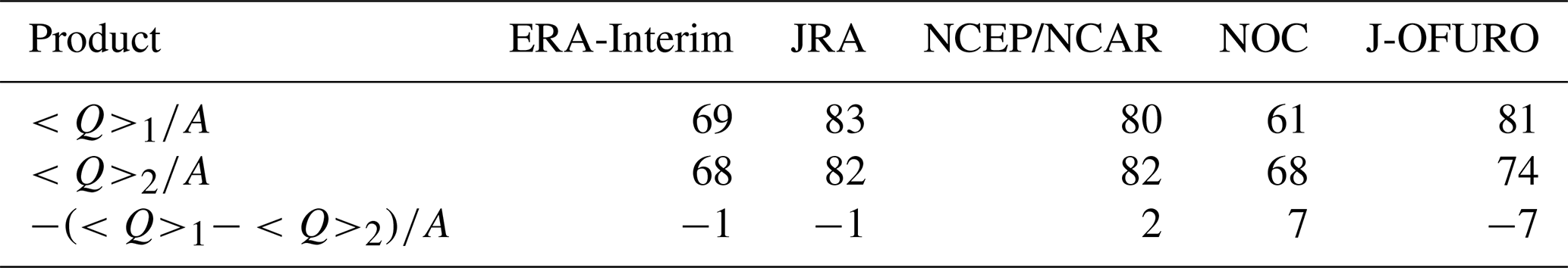
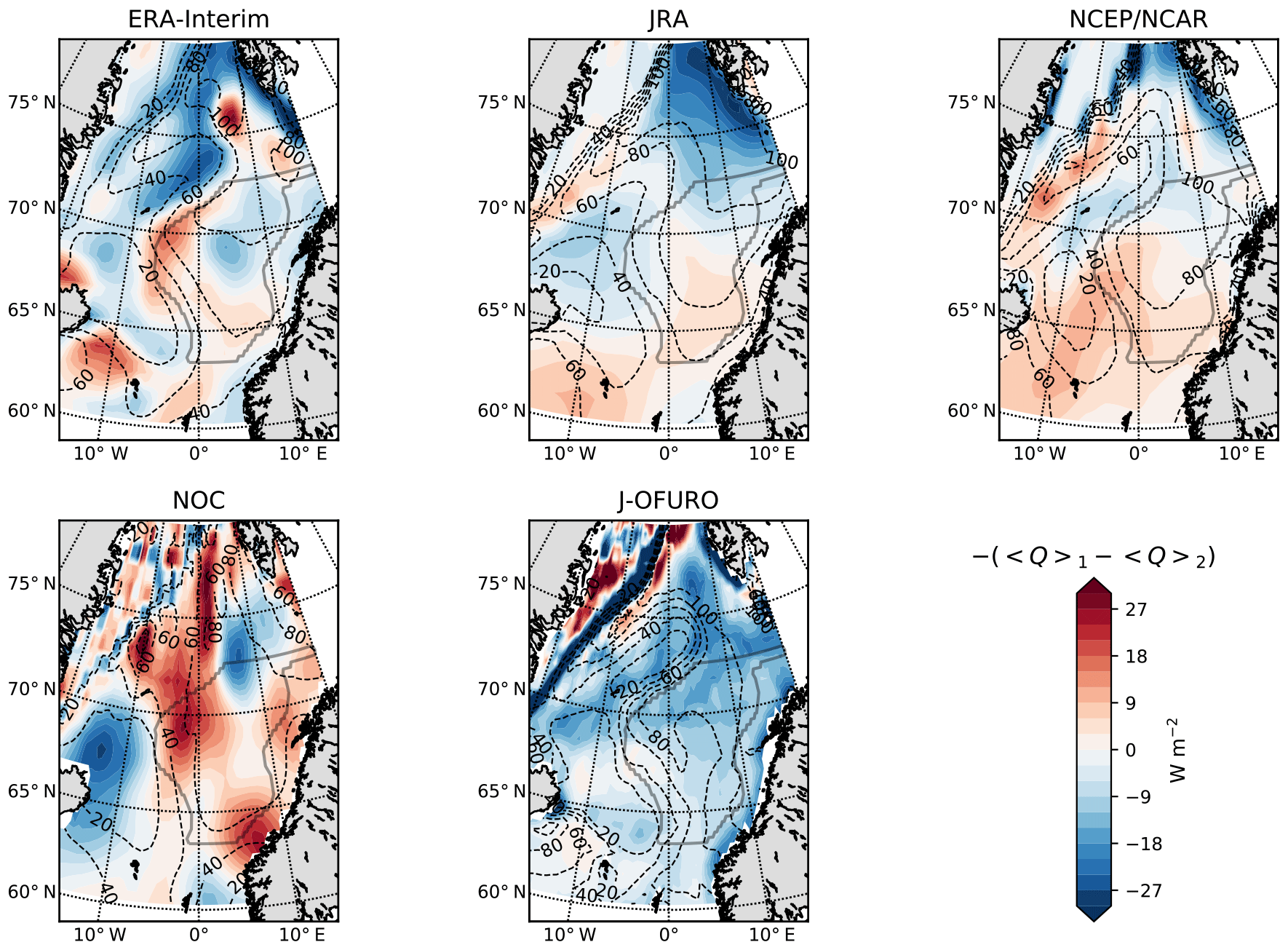
Figure 5Net surface heat flux Q (W m−2), defined positive upwards, for five different products (ERA-Interim, JRA-55, NCEP/NCAR, NOC Surface Flux Dataset and J-OFURO). Shading represents the difference between the periods 1993–2002 and 2004–2013, i.e. , overlaid by the climatological mean net surface heat flux 1993–2013 (dashed contours). The solid grey line depicts the AW domain (cf. Fig. 1).
Several observational studies have found that the surface heat flux can only explain a smaller part of the low-frequency variations in the AW heat content in the Nordic Seas (Carton et al., 2011; Skagseth and Mork, 2012; Shi et al., 2017). A study of a physically consistent ocean state estimate also shows that surface heat flux is not the main source of AW heat content interannual variability (Asbjørnsen et al., 2018). Although the surface heat flux data are not conclusive, we argue that the surface heat flux is not the main source of the change in decadal trends. We will thus continue by considering the other possible source in our heat budget, namely the ocean heat convergence. In the next section we will quantify the convergence and try to disentangle the contribution from variations in temperature and transport.
Conceptual model of ocean heat convergence
We will now show that temperature variations in the AW, flowing across the Greenland–Scotland Ridge and into the southern border of the Nordic Seas AW domain, can explain a significant fraction of the observed heat content variability. To demonstrate this, we model ocean heat convergence as
where Ti∕To is the temperature of the in/outflowing AW and Ψ is the volume transport. Using this, the heat budget in Eq. (8) becomes
We write the variables in the heat budget as a sum of a time-mean part (overbar) and a time varying part (prime), (), and this is done similarly for Ψ and Q. Using these definitions and neglecting the nonlinear term, we obtain
where we have used the fact that the linearized steady-state heat budget is . Further, we set
where T′ is the mean AW temperature anomaly. We will now make two simplifying assumptions. First, since the centre of mass of the AW is located near the Lofoten Basin, close to the northern boundary of our AW domain, we assume that the outflow temperature is approximately equal to the mean AW temperature anomaly T′(t). Second, based on the discussion of the surface heat flux in Sect. 3.2 we will here assume that Q′ is small and thereby limit the analysis to the ocean heat convergence. Using these two simplifications in Eqs. (13) and (14), we obtain the following equation for the mean AW temperature anomaly:
Here, the terms on the righthand side are the forcings due to anomalies in inflow temperature and AW volume transport, respectively. Taking an Atlantic Water area and depth of m2 and ∼700 m, respectively, and Sv (Mork and Skagseth, 2010) gives an e-folding timescale τ∼3 years, which is comparable to published estimates of AW residence times of 3 to 4 years (Koszalka et al., 2013; Broomé and Nilsson, 2018).
Equation (15) is based on the reasonable assumption that the low-frequency ocean heat convergence is dominated by changes in the AW circulation, rather than in air–sea heat fluxes. To examine if variations in temperature or transport dominate the variation in heat convergence, we note that the ratio between the second and first term on the righthand side of Eq. (15) is
This is the ratio between the two driving terms, and if it is small, temperature anomalies dominate over transport anomalies in the ocean heat convergence; the converse occurs when the ratio is large. The Svinøy section is roughly located at the upstream border of our Atlantic Water domain. Here, the mean AW transport is Sv (Mork and Skagseth, 2010), and can be estimated from the steady-state heat budget (Eq. 12) as ; taking W m−2 (see Table 1) gives ∘C. Further, measurements in the Svinøy section indicate low-frequency flow and temperature anomalies (>5 years) that give and (estimated from Fig. 7 in Mork and Skagseth, 2010). This gives a value of about 0.7 for the ratio in Eq. (16), suggesting that variations in temperature can be slightly more important than variations in volume flow. We obtain similar results using observations from the Faroe–Shetland Channel (Berx et al., 2013; Bringedal et al., 2018; Østerhus et al., 2019). We note that per unit area in the AW domain, the term in Eq. (13) gives a heat convergence of 40 W m−2 for a ΔT′ anomaly of 1 ∘C. Thus, a difference in inflow and outflow temperatures less than 0.5 ∘C could explain the observed increase in heat content from the mid-1990s to around 2004.
Our considerations show that AW temperature variations can be as important for the ocean heat convergence as variations in AW volume transport. However, the ocean heat transport variations in sections across the AW, such as the Svinøy section, tend to be dominated by variations in the volume transport (Orvik and Skagseth, 2005; Asbjørnsen et al., 2018). The reason is that there is a net volume transport across the sections, which requires the heat transport to be defined relative to a reference temperature. This reference temperature, characterizing a return flow, is usually taken to be 0 ∘C for AW heat transport in the Nordic Seas (Orvik and Skagseth, 2005). Using a reference temperature of 0 ∘C to estimate the heat transport anomaly in Eq. (13) gives an effective temperature difference ∘C (the mean temperature of the section in degrees Celsius), rather than ∘C (the temperature difference between in- and out-flowing water) as used here for estimating the ocean heat convergence.
We also note that observations of volume transport at the southern inflows to the Nordic Seas indicate no clear decadal trends over the time period (Berx et al., 2013; Hansen et al., 2015; Bringedal et al., 2018; Østerhus et al., 2019). The volume transport can also be estimated from the slope of SSH (Chafik et al., 2015). Over the slope in the FSC, such a barotropic calculation (not shown) gives a mean transport of just under 4 Sv (consistent with the 4.1 Sv direct estimates by Rossby and Flagg, 2012), with monthly estimates ranging from 0 to 8 Sv but no clear decadal trends. Accordingly, it is unlikely that variations in AW volume transport and air–sea fluxes have been the main drivers of the observed trends in heat content and SSH in the eastern Nordic Seas in the period presently considered.
Motivated by these considerations, we examine how well the simple model defined by Eq. (15) can reproduce the evolution of the mean AW temperature anomaly, given the inflow temperature as the only forcing. We note that by converting the observed heat content anomaly (by dividing it by cpVAW) to a temperature anomaly, the left-hand side of Eq. (15) can be used to compute the total model forcing, defined by , representing the forcing required to reproduce the observations. This allows us to examine both how well the inflow temperature reproduces the total model forcing and the observed AW heat content variations. For this purpose, we estimate the AW inflow temperature from sea surface EN4 temperatures in the Faroe–Shetland Channel and in the Svinøy section from 1955 up to the present and integrate Eq. (15) numerically forward in time. In the calculations, we use the e-folding timescales (τ) 2.5, 3.0 and 4.0 years, which are in the range of estimated residence times in the presently defined AW domain (Koszalka et al., 2013; Broomé and Nilsson, 2018). This range of τ implies that the temperature/heat-content anomaly evolution in the model is influenced by the upstream temperature history a couple of years back in time. The heat content is related to the temperature by Eq. (14), using a mean depth of the AW layer of 700 m (note that the depth level 657 m in the EN4 data, used earlier, is the level closest to 700 m).
Figure 6 shows the proxies for the AW inflow temperature forcing and the resulting modelled heat content anomaly as well as the low-pass-filtered AW heat content anomaly estimated from the EN4 data (from Fig. 4). Figure 6a also shows the total model-forcing temperature anomaly (the righthand side of Eq. 15) needed to reproduce the observed heat content variations. For easy comparison, the heat content anomalies have been set to zero in 1993. The results based on the Svinøy section temperature (results are similar when the Faroe–Shetland Channel temperature is used) show that the simple model reproduces the main features of the low-frequency evolution of the AW heat anomaly. For all three values of τ, the modelled heat content anomaly increases from the mid-1990s to the mid-2000s with a more stagnant period following, in broad agreement with the observations. In effect, the model acts as a low-pass filter on the driving inflow temperature , suppressing variability with timescales shorter than about 4 years. Thus, the model heat anomaly is mainly forced by the general increase in the inflow temperature up to around 2003 and the more constant inflow temperature in the period thereafter. There are some obvious differences between the model and the observational estimate of the heat content. Specifically, the increase in the heat anomaly in the data from around 1997 to 2004 is weaker and possibly delayed by a couple of years in the model. A strengthening of the AW volume transport of some 10 %–20 % or a decreased surface heat loss during this period may explain the deviation between the simple model and the data-based estimate of the heat content anomaly. By comparing the forcing from the inflow temperature variations to the total model forcing (Fig. 6a), we note that the total model forcing is higher from around 1998 to 2002. Current metre observations show that the AW inflow to the Nordic Seas (Bringedal et al., 2018; Østerhus et al., 2019) and through the Svinøy section (Mork and Skagseth, 2010) increased some 20 % from around 1995 to 2000. This makes variations in AW volume transport a plausible cause for why the heat content increase is weaker in the conceptual model than in the observations in the earlier period. Nevertheless, despite the rather drastic simplifications of the conceptual model, this calculation shows that the variations in the inflow temperature at the southern boundary are important for the observed low-frequency heat content variability in the AW domain.

Figure 6(a) Sea surface EN4 temperature anomaly (∘C) in the Faroe–Shetland Channel (FSC, red) and in the Svinøy section (Svinoy, blue), used as proxies for the inflow temperature anomaly . The dashed black line shows the total model forcing temperature needed to reproduce the observed AW heat content anomaly (black line in b). (b) Modelled AW heat content anomaly (blue), which is obtained by integrating Eq. (15) forward in time, using the Svinøy section temperatures and the e-folding timescales (τ) equal to 2.5, 3.0 and 4.0 years. The black line shows the heat content AW anomaly estimated from the EN4 data; the same data are shown in Fig. 4, but here they are low-pass-filtered with a 24-month running mean.
3.3 Connection to the upstream subpolar North Atlantic
Since our results suggest that local air–sea heat fluxes cannot explain the decadal heat content variability and that ocean advection of temperature anomalies from the south is the main cause, it is reasonable to assume a close connection to the subpolar North Atlantic (SPNA). In this regard, several studies have documented a link between SPNA temperature variability and the Nordic Seas, mediated by advection of temperature anomalies along the eastern branch of the North Atlantic Current (Chepurin and Carton, 2012; Årthun and Eldevik, 2016; Årthun et al., 2017; Langehaug et al., 2019). We will now consider if such an advective connection can explain Nordic Seas AW temperature variations from the period from around 1993 to 2016.
Figure 7, based on empirical orthogonal function analysis (Hannachi et al., 2007), shows that the leading mode of temperature variability in the SPNA (explained variance is 70 %), of both surface and subsurface temperatures down to ∼400 m, is dominated by pronounced decadal variability. However, while the decadal temperature changes in the eastern Nordic Seas (Fig. 7a) track those in the SPNA (Fig. 7b) during the 1993–2004 period, a clear disconnection is seen after 2005. Consistent with the SSH and heat content analysis (e.g. Fig. 4), Fig. 7 shows that while the SPNA has been cooling since the mid-2000s, the Nordic Seas have not. This disconnection suggests a weak relationship between the eastern Nordic Seas and changes in the SPNA during its cooling phase (∼mid-2000s to 2016) but a strong connection, as shown here and documented by many studies (Hátún et al., 2005; Skagseth and Mork, 2012), during the warming phase of the SPNA (∼early 1990s to mid-2000s).
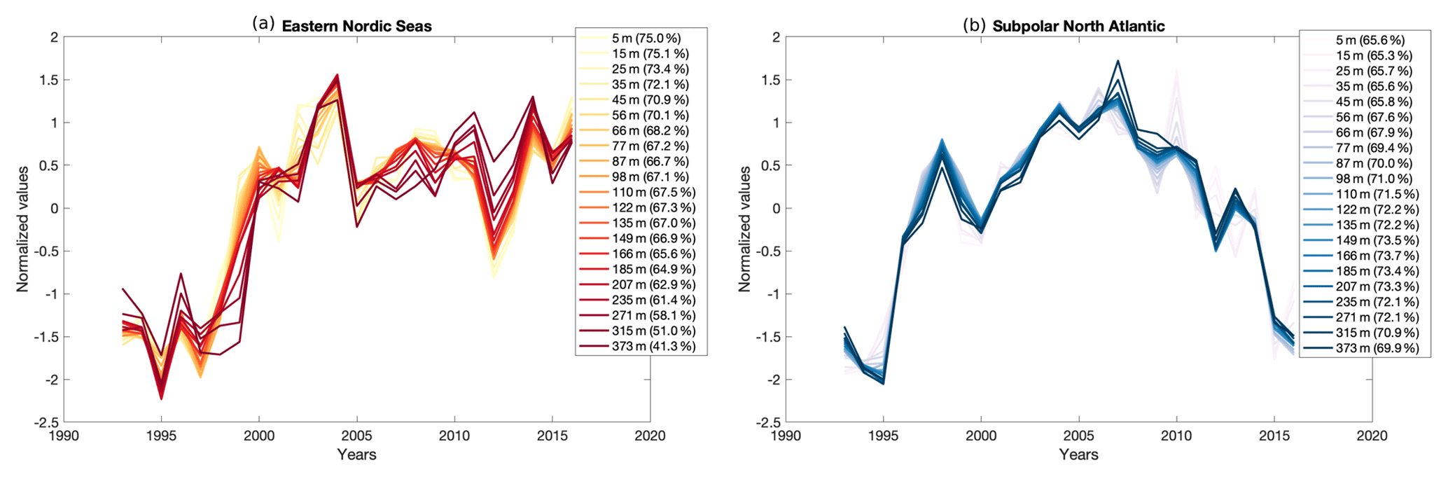
Figure 7The leading mode of variability in the deseasonalized (no trend removed) and annually averaged temperature anomalies down to 400 m in (a) the eastern Nordic Seas (10∘ W–15∘ E, 62–72∘ N) and (b) the subpolar North Atlantic (45–5∘ W, 55–65∘ N) for the 1993–2016 period using EN4. The explained variance in every depth can be seen in parentheses in the figure legend.
This weakened (enhanced) connection between the SPNA and the Nordic Seas during the recent cooling (warming) phase may be explained by the horizontal circulation and hence the shape of the subpolar gyre/front in the eastern SPNA. As the subpolar gyre strengthens (weakens) during the cooling (warming) phase, in response to several years of strong (weak) wind-stress curl (Häkkinen et al., 2011), it also expands (contracts) in size, and the subpolar front shifts eastwards (westwards), which, in turn, leads to a smaller (larger) fraction of subtropical water masses spreading along the eastern boundary, across the Greenland–Scotland Ridge and into the Nordic Seas. This view is supported by a spatial correlation analysis between the leading mode of temperature variability in the Nordic Seas at 100 m compared with that in the wider North Atlantic, shown in Fig. 8. The resulting pattern indicates that the relationship with the SPNA is only strong and significant along the subtropical path in the eastern subpolar gyre and around its rim rather than in the central SPNA, where the correlation is weak, negative and not significant. It is thus possible that the contraction and expansion of the subpolar gyre, through its control of the northward access of warm and saline subtropical waters in the eastern subpolar gyre (Hátún et al., 2005; Häkkinen et al., 2011; Chafik et al., 2019), may have regulated the observed time-varying connection between the SPNA and the Nordic Seas (Figs. 4 and 7) and hence the rate of ocean heat content and sea surface height change in the eastern Nordic Seas on decadal scales.
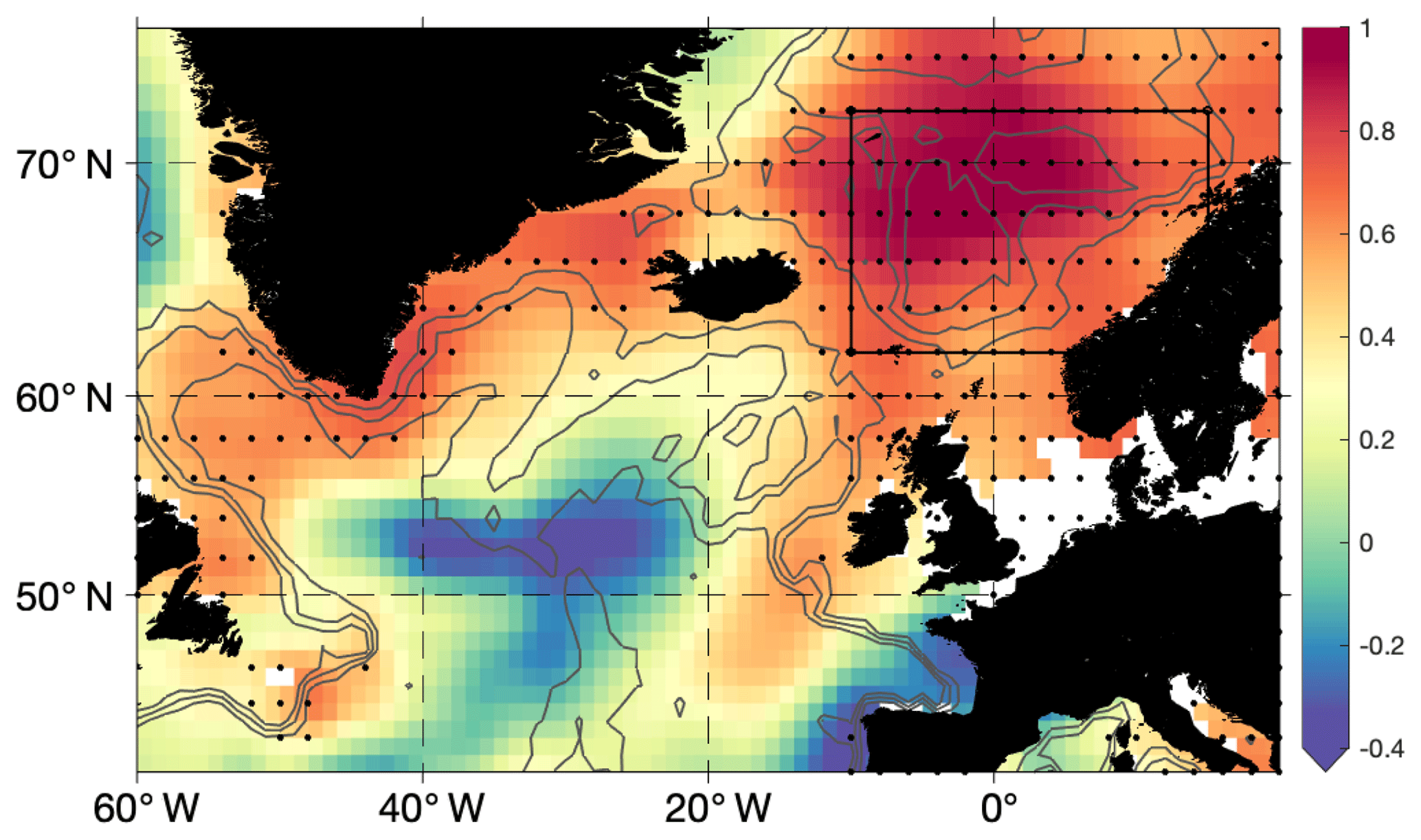
Figure 8Correlation analysis between the leading mode of temperature variability at 100 m in the eastern Nordic Seas (see black box and Fig. 7a) against temperature anomalies at every grid point at the same depth. The data (not detrended) have been deseasonalized and annually averaged before the analysis. Black dots indicate significance at the 95 % confidence level according to a random phase test (Ebisuzaki, 1997). Grey contours depict the 1000, 2000 and 3000 m depth contours.
The subpolar gyre linkage discussed above together with the simple model in Sect. 3.2.1, which only includes inflow temperature variations, suggests that air–sea fluxes could not have caused the observed shift in decadal heat content trends. However, this does not rule out that atmospheric circulation anomalies may also have helped to maintain warm ocean temperatures in the Nordic Seas since the mid-2000s, resulting in the stagnant period instead of the cooling seen in the SPNA. This may be consistent with conclusions from a recent study by Asbjørnsen et al. (2018), which reported that local forcing from air–sea heat fluxes are important for modulating the anomalies on their northward path. However, it is also possible that the ongoing cooling in the SPNA (Chafik et al., 2019) had simply not yet reached the Nordic Seas at the end of 2016. Although we have only speculated the cause for this stagnant period, our simple model of heat convergence reproduced the decadal heat content variability in the eastern Nordic Seas reasonably well, despite the observed disconnection from the SPNA. This important result thus suggests that temperature conditions in the northeastern Atlantic and at the Greenland–Scotland Ridge are key in setting the decadal variability in ocean heat content and SSH changes in the eastern Nordic Seas.
In this study of the Atlantic Water (AW) of the Nordic Seas, we analyse changes in sea surface height (SSH) on decadal timescales since 1993 and investigate underlying mechanisms. Over the full period of satellite observations of SSH, 1993–2017, there is a general positive trend coincident with a warming of AW in the eastern Nordic Seas. We identify a shift in the trend of SSH in the AW, from a decade with a strong positive trend to a more stagnant decade. A similar change in trend is also found in the heat content of the AW. We argue that the steric height changes related to the variation in heat content is the main reason for the observed decadal changes in SSH trends and further investigate whether the source of the decadal changes is local or remote.
Through a simple heat budget adapted to the AW, we discuss three possible reasons for the decadal variations in heat content: a difference in net surface heat flux between the two periods (local source) and a difference in either volume transport or temperature of the AW inflow at the southern boundary (remote source). We conclude that the most plausible cause of changes in SSH and heat content on decadal timescales is remote and advected with the Atlantic source waters entering the Nordic Seas over the Greenland–Scotland Ridge. We also conclude that decadal-scale changes in inflow temperature, rather than in volume transport, have dominated during the period considered in this study. A quantitative estimate of the relative contributions from volume transport and temperature in the heat transport shows that a difference in inflow temperature of 0.5 ∘C is enough to explain the decadal changes in heat content. Furthermore, we construct a simplified conceptual heat budget model to forecast the AW heat content based on a single measurement of temperature at one of the main inflow regions to the Nordic Seas, i.e. the Faroe-Shetland Channel. The model is able to reproduce the main features of the observed decadal changes in AW heat content and SSH in time and magnitude. Interestingly, the AW in the Nordic Seas has not experienced the same reversal of trends as the upstream central subpolar North Atlantic but instead seems more related to the rim of the SPNA and maintains warm ocean temperatures and high SSH during the period considered.
We have connected decadal variability to upstream conditions, which has implications for decadal climate predictability in the Nordic Seas. It is equally important to note that the conditions observed in the AW of the Nordic Seas can have an impact further downstream (Polyakov et al., 2017; Smedsrud et al., 2013; Sandø et al., 2010). For example, discussions in the past few years have referred to an “Atlantification” of the Barents Sea and Arctic Ocean as a cause of sea ice loss (see e.g. Årthun et al., 2012; Polyakov et al., 2017), highlighting the importance of upstream AW conditions. Last but not least, this study shows that the satellite absolute dynamic topography can be used to study decadal variability in heat content, which is useful since the satellite data are accessible, have no summer bias, and generally have better and more even resolution in time and space than hydrography.
The absolute dynamic topography data are available from http://marine.copernicus.eu/services-portfolio/access-to-products/ (last access: 10 August 2018, Copernicus Marine Service, 2018) with the product identifier: SEALEVEL_GLO_PHY_L4_REP_OBSERVATIONS_008_047. The EN4.2.0 hydrographic data are available from https://www.metoffice.gov.uk/hadobs/en4/ (last access: 20 November 2018, Met Office Hadley Centre, 2018). ERA-interim is available through ECMWF: https://www.ecmwf.int/en/forecasts/datasets/reanalysis-datasets/era-interim (last access: 25 June 2019, ECMWF, 2019). NCEP/NCAR is available through NOAA: https://psl.noaa.gov/data/gridded/data.ncep.reanalysis.html (last access: 25 June 2019, NOAA NCEP, 2019). The JRA reanalysis (JMA, 2013) along with the NOC surface flux (National Oceanography Centre Southampton, 2008) are available from the Research Data Archive: https://rda.ucar.edu/ (last access: 25 May 2018). The J-OFURO (2019) data are available from https://j-ofuro.scc.u-tokai.ac.jp/en/ (last access: 25 June 2019).
SB carried out the analysis from an original idea of LC and with continuous input from LC and JN. SB wrote the bulk of the paper, with JN as main author of Sect. 3.2 and LC as the main author of Sect. 3.3.
The authors declare that they have no conflict of interest.
We thank Jonas Nycander and two anonymous reviewers for valuable comments.
This research has been supported by the Swedish National Space Agency (grant nos. 133/17 and 111/16).
The article processing charges for this open-access
publication were covered by Stockholm University.
This paper was edited by Trevor McDougall and reviewed by two anonymous referees.
Årthun, M. and Eldevik, T.: On anomalous ocean heat transport toward the Arctic and associated climate predictability, J. Climate, 29, 689–704, 2016. a, b
Årthun, M., Eldevik, T., Smedsrud, L. H., Skagseth, Ø., and Ingvaldsen, R.: Quantifying the influence of atlantic heat on Barents sea ice variability and retreat, J. Climate, 25, 4736–4743, 2012. a
Årthun, M., Eldevik, T., Viste, E., Drange, H., Furevik, T., Johnson, H. L., and Keenlyside, N. S.: Skillful prediction of northern climate provided by the ocean, Nat. Commun., 8, 15875, https://doi.org/10.1038/ncomms16152, 2017. a, b
Asbjørnsen, H., Årthun, M., Skagseth, Ø., and Eldevik, T.: Mechanisms of ocean heat anomalies in the Norwegian Sea, J. Geophys. Res.-Oceans, 124, 2908–2923, 2018. a, b, c, d
Becker, J. J., Sandwell, D. T., Smith, W. H. F., Braud, J., Binder, B., Depner, J., Fabre, D., Factor, J., Ingalls, S., Kim, S.-H., Ladner, R., Marks, K., Nelson, S., Pharaoh, A., Sharman, G., Trimmer, R., Von Rosenburg, J., Wallace, G., and Weatherall, P.: Global Bathymetry and Elevation Data at 30 Arc Seconds Resolution: SRTM30_PLUS, revised for Mar. Geod., 32, 355–371, 2009. a, b, c
Berry, D. I. and Kent, E. C.: A new air–sea interaction gridded dataset from ICOADS with uncertainty estimates, B. Am. Meteorol. Soc., 90, 645–656, 2009. a
Berry, D. I. and Kent, E. C.: Air–sea fluxes from ICOADS: The construction of a new gridded dataset with uncertainty estimates, Int. J. Climatol., 31, 987–1001, 2011. a
Berx, B., Hansen, B., Østerhus, S., Larsen, K. M., Sherwin, T., and Jochumsen, K.: Combining in situ measurements and altimetry to estimate volume, heat and salt transport variability through the Faroe–Shetland Channel, Ocean Sci., 9, 639–654, https://doi.org/10.5194/os-9-639-2013, 2013. a, b
Bringedal, C., Eldevik, T., Skagseth, Ø., Spall, M. A., and Østerhus, S.: Structure and Forcing of Observed Exchanges across the Greenland–Scotland Ridge, J. Climate, 31, 9881–9901, https://doi.org/10.1175/JCLI-D-17-0889.1, 2018. a, b, c
Broomé, S. and Nilsson, J.: Stationary Sea Surface Height anomalies in cyclonic boundary currents: Conservation of potential vorticity and deviations from strict topographic steering, J. Phys. Oceanogr., 46, 2437–2456, https://doi.org/10.1175/JPO-D-15-0219.1, 2016. a, b, c
Broomé, S. and Nilsson, J.: Shear dispersion and delayed propagation of temperature anomalies along the Norwegian Atlantic Slope Current, Tellus A, 70, 1–13, 2018. a, b
Carton, J. A., Chepurin, G. A., Reagan, J., and Häkkinen, S.: Interannual to decadal variability of Atlantic Water in the Nordic and adjacent seas, J. Geophys. Res., 116, C11035, https://doi.org/10.1029/2011JC007102, 2011. a, b
Carton, J. A., Chepurin, G. A., Chen, L., and Grodsky, S. A.: Improved global net surface heat flux, J. Geophys. Res.-Oceans, 123, 3144–3163, 2018. a
Chafik, L. and Rossby, T.: Volume, heat and freshwater divergences in the subpolar North Atlantic suggest the Nordic Seas as key to the state of the meridional overturning circulation, Geophys. Res. Lett., 46, 4799–4808, 2019. a
Chafik, L., Nilsson, J., Skagseth, Ø., and Lundberg, P.: On the Flow of Atlantic Water and Temperature Anomalies in the Nordic Seas Towards the Arctic Ocean, J. Geophys. Res.-Oceans, 120, 7897–7918, https://doi.org/10.1002/2015JC011012, 2015. a, b, c
Chafik, L., Nilsen, J. E. Ø., Dangendorf, S., Reverdin, G., and Frederikse, T.: North Atlantic Ocean Circulation and Decadal Sea Level Change During the Altimetry Era, Scientific Reports, 9, 1041, https://doi.org/10.1038/s41598-018-37603-6, 2019. a, b, c, d
Chepurin, G. A. and Carton, J. A.: Subarctic and Arctic sea surface temperature and its relation to ocean heat content 1982–2010, J. Geophys. Res., 117, C06019, https://doi.org/10.1029/2011JC007770, 2012. a
Copernicus Marine Service: http://marine.copernicus.eu/services-portfolio/access-to-products/, last access: 10 August 2018. a
Dee, D. P., Uppala, S., Simmons, A., Berrisford, P., Poli, P., Kobayashi, S., Andrae, U., Balmaseda, M., Balsamo, G., Bauer, P., Bechtold, P., Beljaars, A., van de Berg, L., Bidlot, J.-R., Bormann, N., Delsol, C., Dragani, R., Fuentes, M., Geer, A. J., Haimberger, L., Healy, S., Hersbach, H., Hólm, E. V., Isaksen, L., Kållberg, P. W., Köhler, M., Matricardi, M., McNally, A., Monge-Sanz, B. M., Morcrette, J.-J., Peubey, C., de Rosnay, P., Tavolato, C., Thépaut, J.-N., and Vitart, F.: The ERA-Interim reanalysis: Configuration and performance of the data assimilation system, Q. J. Roy. Meteor. Soc., 137, 553–597, 2011. a
Drange, H., Dokken, T., Furevik, T., Gerdes, R., Berger, W., Nesje, A., Orvik, K. A., Skagseth, O., Skjelvan, I., and Osterhus, S.: The Nordic seas: an overview, in: The Nordic Seas: An Integrated Perspective, edited by: Drange, H., Dokken, T., Furevik, T., Gerdes, R., and Berger, W., Geoph. Monog. Series, 158, 1–10, 2005. a
Dugstad, J., Fer, I., LaCasce, J., Sanchez de La Lama, M., and Trodahl, M.: Lateral Heat Transport in the Lofoten Basin: Near-Surface Pathways and Subsurface Exchange, J. Geophys. Res.-Oceans, 124, 2992–3006, https://doi.org/10.1029/2018JC014774, 2019. a, b
Ebisuzaki, W.: A method to estimate the statistical significance of a correlation when the data are serially correlated, J. Climate, 10, 2147–2153, 1997. a
ECMWF: https://www.ecmwf.int/en/forecasts/datasets/reanalysis-datasets/era-interim, last access: 25 June 2019. a
Eldevik, T., Nilsen, J. E. Ø., Iovino, D., Olsson, K. A., Sandø, A. B., and Drange, H.: Observed sources and variability of Nordic seas overflow, Nat. Geosci., 2, 406–410, 2009. a
Furevik, T.: On anomalous sea surface temperatures in the Nordic Seas, J. Climate, 13, 1044–1053, 2000. a
Furevik, T., Mauritzen, C., and Ingvaldsen, R.: The flow of Atlantic water to the Nordic Seas and Arctic Ocean, in: Arctic alpine ecosystems and people in a changing environment, edited by: Ørbæk, J. B., Kallenborn, R., Tombre, I., Hegseth, E. N., Falk-Petersen, S., and Hoel, A. H., Springer, Berlin, Heidelberg, 123–146, 2007. a
Gill, A. and Niller, P.: The theory of the seasonal variability in the ocean, Deep Sea Research and Oceanographic Abstracts, 20, 141–177, 1973. a, b, c
Glessmer, M. S., Eldevik, T., Våge, K., Nilsen, J. E. Ø., and Behrens, E.: Atlantic origin of observed and modelled freshwater anomalies in the Nordic Seas, Nat. Geosci., 7, 801–805, 2014. a
Good, S. A., Martin, M. J., and Rayner, N. A.: EN4: Quality controlled ocean temperature and salinity profiles and monthly objective analyses with uncertainty estimates, J. Geophys. Res.-Oceans, 118, 6704–6716, 2013. a
Gouretski, V. and Reseghetti, F.: On depth and temperature biases in bathythermograph data: Development of a new correction scheme based on analysis of a global ocean database, Deep-Sea Res. Pt. I, 57, 812–833, 2010. a
Häkkinen, S., Rhines, P. B., and Worthen, D. L.: Atmospheric blocking and Atlantic multidecadal ocean variability, Science, 334, 655–659, 2011. a, b
Hannachi, A., Jolliffe, I. T., and Stephenson, D. B.: Empirical orthogonal functions and related techniques in atmospheric science: A review, Int. J. Climatol., 27, 1119–1152, https://doi.org/10.1002/joc.1499, 2007. a
Hansen, B. and Østerhus, S.: North Atlantic–Nordic Seas exchanges, Prog. Oceanogr., 45, 109–208, 2000. a
Hansen, B., Larsen, K. M. H., Hátún, H., Kristiansen, R., Mortensen, E., and Østerhus, S.: Transport of volume, heat, and salt towards the Arctic in the Faroe Current 1993–2013, Ocean Sci., 11, 743–757, https://doi.org/10.5194/os-11-743-2015, 2015. a
Hátún, H., Sandø, A. B., Drange, H., Hansen, B., and Valdimarsson, H.: Influence of the Atlantic subpolar gyre on the thermohaline circulation, Science, 309, 1841–1844, 2005. a, b, c
JMA (Japan Meteorological Agency): JRA-55: Japanese 55-year Reanalysis, Monthly Means and Variances, Research Data Archive at the National Center for Atmospheric Research, Computational and Information Systems Laboratory, Boulder CO, https://doi.org/10.5065/D60G3H5B, 2013. a
J-OFURO: https://j-ofuro.scc.u-tokai.ac.jp/en/, last access: 25 June 2019. a
Kalnay, E., Kanamitsu, M., Kistler, R., Collins, W., Deaven, D., Gandin, L., Iredell, M., Saha, S., White, G., Woollen, J., Zhu, Y., Chelliah, M., Ebisuzaki, W., Higgins, W., Janowiak, J., Mo, K. C. Ropelewski, C., Wang, J., Leetmaa, A., Reynolds, R., Jenne, R., and Joseph, D.: The NCEP/NCAR 40-year reanalysis project, B. Am. Meteorol. Soc., 77, 437–472, 1996. a
Kobayashi, S., Ota, Y., Harada, Y., Ebita, A., Moriya, M., Onoda, H., Onogi, K., Kamahori, H., Kobayashi, C., Endo, H., Miyaoka, K., and Takahashi, K.: The JRA-55 reanalysis: General specifications and basic characteristics, J. Meteorol. Soc. Jpn., Ser. II, 93, 5–48, 2015. a
Köhl, A.: Generation and stability of a quasi-permanent vortex in the Lofoten Basin, J. Phys. Oceanogr., 37, 2637–2651, 2007. a, b
Koszalka, I., LaCasce, J., and Mauritzen, C.: In pursuit of anomalies–Analyzing the poleward transport of Atlantic Water with surface drifters, Deep-Sea Res. Pt. II, 85, 96–108, 2013. a, b, c
Langehaug, H. R., Sandø, A. B., Årthun, M., and Ilıcak, M.: Variability along the Atlantic water pathway in the forced Norwegian Earth System Model, Clim. Dynam., 52, 1211–1230, 2019. a
Mauritzen, C.: Production of dense overflow waters feeding the North Atlantic across the Greenland-Scotland Ridge. Part 1: Evidence for a revised circulation scheme, Deep-Sea Res. Pt. I, 43, 769–806, 1996. a, b
Met Office Hadley Centre: https://www.metoffice.gov.uk/hadobs/en4/, last access: 20 November 2018. a
Mork, K. A. and Skagseth, Ø.: A quantitative description of the Norwegian Atlantic Current by combining altimetry and hydrography, Ocean Sci., 6, 901–911, https://doi.org/10.5194/os-6-901-2010, 2010. a, b, c, d
Mork, K. A., Skagseth, Ø., Ivshin, V., Ozhigin, V., Hughes, S. L., and Valdimarsson, H.: Advective and atmospheric forced changes in heat and fresh water content in the Norwegian Sea, 1951–2010, Geophys. Res. Lett., 41, 6221–6228, 2014. a, b
Mork, K. A., Skagseth, Ø., and Søiland, H.: Recent warming and freshening of the Norwegian Sea observed by Argo data, J. Climate, 32, 3695–3705, 2019. a
National Oceanography Centre Southampton (NOCS): NOCS Surface Flux Dataset v2.0, Research Data Archive at the National Center for Atmospheric Research, Computational and Information Systems Laboratory, Boulder CO, https://doi.org/10.5065/V8E1-ZD23, 2008. a
Nilsson, J., Walin, G., and Broström, G.: Thermohaline circulation induced by bottom friction in sloping-boundary basins, J. Mar. Res., 63, 705–728, 2005. a
NOAA National Center for Environmental Prediction (NOAA NCEP): https://psl.noaa.gov/data/gridded/data.ncep.reanalysis, last access: 25 June 2019. a
Oliphant, T. E.: Python for Scientific Computing, Comput. Sci. Eng., 9, 10–20, https://doi.org/10.1109/MCSE.2007.58, 2007. a
Orvik, K. A. and Niiler, P.: Major pathways of Atlantic water in the northern North Atlantic and Nordic Seas toward Arctic, Geophys. Res. Lett., 29, 1896, https://doi.org/10.1029/2002GL015002, 2002. a, b
Orvik, K. A. and Skagseth, Ø.: Heat flux variations in the eastern Norwegian Atlantic Current toward the Arctic from moored instruments, 1995–2005, Geophys. Res. Lett., 32, L14610, https://doi.org/10.1029/2005GL023487, 2005. a, b
Østerhus, S., Woodgate, R., Valdimarsson, H., Turrell, B., de Steur, L., Quadfasel, D., Olsen, S. M., Moritz, M., Lee, C. M., Larsen, K. M. H., Jónsson, S., Johnson, C., Jochumsen, K., Hansen, B., Curry, B., Cunningham, S., and Berx, B.: Arctic Mediterranean exchanges: a consistent volume budget and trends in transports from two decades of observations, Ocean Sci., 15, 379–399, https://doi.org/10.5194/os-15-379-2019, 2019. a, b, c
Piecuch, C. G., Ponte, R. M., Little, C. M., Buckley, M. W., and Fukumori, I.: Mechanisms underlying recent decadal changes in subpolar North Atlantic Ocean heat content, J. Geophys. Res.-Oceans, 122, 7181–7197, 2017. a
Polyakov, I. V., Pnyushkov, A. V., Alkire, M. B., Ashik, I. M., Baumann, T. M., Carmack, E. C., Goszczko, I., Guthrie, J., Ivanov, V. V., Kanzow, T., Krishfield, R., Kwok, R., Sundfjord, A., Morison, J., Rember, R., and Yulin, A.: Greater role for Atlantic inflows on sea-ice loss in the Eurasian Basin of the Arctic Ocean, Science, 356, 285–291, 2017. a, b
Pujol, M.-I., Faugère, Y., Taburet, G., Dupuy, S., Pelloquin, C., Ablain, M., and Picot, N.: DUACS DT2014: the new multi-mission altimeter data set reprocessed over 20 years, Ocean Sci., 12, 1067–1090, https://doi.org/10.5194/os-12-1067-2016, 2016. a
Raj, R. P., Chafik, L., Nilsen, J. E. Ø., Eldevik, T., and Halo, I.: The Lofoten Vortex of the Nordic Seas, Deep-Sea Res. Pt. I, 96, 1–14, 2015. a
Richter, K. and Maus, S.: Interannual variability in the hydrography of the Norwegian Atlantic Current: Frontal versus advective response to atmospheric forcing, J. Geophys. Res., 116, C12031, https://doi.org/10.1029/2011JC007311, 2011. a, b
Robson, J., Ortega, P., and Sutton, R.: A reversal of climatic trends in the North Atlantic since 2005, Nat. Geosci., 9, 513–517, 2016. a
Rossby, T. and Flagg, C. N.: Direct measurement of volume flux in the Faroe-Shetland Channel and over the Iceland-Faroe Ridge, Geophys. Res. Lett., 39, L07602, https://doi.org/10.1029/2012GL051269, 2012. a
Ruiz-Barradas, A., Chafik, L., Nigam, S., and Häkkinen, S.: Recent subsurface North Atlantic cooling trend in context of Atlantic decadal-to-multidecadal variability, Tellus A, 70, 1–19, 2018. a
Sandø, A. B., Nilsen, J. E. Ø., Gao, Y., and Lohmann, K.: Importance of heat transport and local air-sea heat fluxes for Barents Sea climate variability, J. Geophys. Res., 115, C07013, https://doi.org/10.1029/2009JC005884, 2010. a
Segtnan, O., Furevik, T., and Jenkins, A.: Heat and freshwater budgets of the Nordic Seas computed from atmospheric reanalysis and ocean observations, J. Geophys. Res., 116, C11003, https://doi.org/10.1029/2011JC006939, 2011. a
Shi, W., Zhao, J., Lian, X., Wang, X., and Chen, W.: Slowdown of sea surface height rises in the Nordic seas and related mechanisms, Acta Oceanol. Sin., 36, 20–33, https://doi.org/10.1007/s13131-017-1027-x, 2017. a, b, c, d, e
Siegismund, F., Johannessen, J., Drange, H., Mork, K., and Korablev, A.: Steric height variability in the Nordic Seas, J. Geophys. Res., 112, C12010, https://doi.org/10.1029/2007JC004221, 2007. a
Skagseth, Ø. and Mork, K. A.: Heat content in the Norwegian Sea, 1995–2010, ICES J. Mar. Sci., 69, 826–832, 2012. a, b, c, d, e, f
Skagseth, Ø., Furevik, T., Ingvaldsen, R., Loeng, H., Mork, K. A., Orvik, K. A., and Ozhigin, V.: Volume and heat transports to the Arctic Ocean via the Norwegian and Barents Seas, in: Arctic-Subarctic Ocean Fluxes, edited by: Dickson, R. R., Meincke, J., and Rhines, P., Springer Netherlands, 45–64, 2008. a
Smedsrud, L. H., Esau, I., Ingvaldsen, R. B., Eldevik, T., Haugan, P. M., Li, C., Lien, V. S., Olsen, A., Omar, A. M., Otterå, O. H., Risebrobakken, B., Sandø, A. B., Semenov, V. A., and Sorokina, S. A.: The role of the Barents Sea in the Arctic climate system, Rev. Geophys., 51, 415–449, 2013. a
Søiland, H., Chafik, L., and Rossby, T.: On the long-term stability of the Lofoten Basin Eddy, J. Geophys. Res.-Oceans, 121, 4438–4449, https://doi.org/10.1002/2016JC011726, 2016. a
Spall, M. A.: Non-local topographic influences on deep convection: An idealized model for the Nordic Seas, Ocean Model., 32, 72–85, 2010. a
Stammer, D.: Steric and wind-induced changes in TOPEX/POSEIDON large-scale sea surface topography observations, J. Geophys. Res., 102, 20987–21009, 1997. a
Stammer, D., Cazenave, A., Ponte, R. M., and Tamisiea, M. E.: Causes for Contemporary Regional Sea Level Changes, Annu. Rev. Mar. Sci., 5, 21–46, https://doi.org/10.1146/annurev-marine-121211-172406, 2013. a
Tomita, H., Hihara, T., Kako, S., Kubota, M., and Kutsuwada, K.: An introduction to J-OFURO3, a third-generation Japanese ocean flux data set using remote-sensing observations, J. Oceanogr., 75, 171–194, 2019. a
Walin, G., Broström, G., Nilsson, J., and Dahl, O.: Baroclinic boundary currents with downstream decreasing buoyancy: A study of an idealized Nordic Seas system, J. Mar. Res., 62, 517–543, 2004. a
Zweng, M., Reagan, J., Antonov, J., Locarnini, R., Mishonov, A., Boyer, T., Garcia, H., Baranova, O., Johnson, D., Seidov, D., and Biddle, M.: World Ocean Atlas 2013, Volume 2: Salinity, edited by: S. Levitus, and Mishonov, A., NOAA Atlas NESDIS 74, 39 pp., 2013. a