the Creative Commons Attribution 4.0 License.
the Creative Commons Attribution 4.0 License.
 | 26 May 2020
Very high-resolution modelling of submesoscale turbulent patterns and processes in the Baltic Sea
Reiner Onken
Burkard Baschek
Ingrid M. Angel-Benavides
In order to simulate submesoscale turbulent patterns and processes (STPPs) and to analyse their properties and dynamics, the Regional Ocean Modeling System (ROMS) was run for June 2016 in a subregion of the Baltic Sea. To create a realistic mesoscale environment, ROMS with 500 m horizontal resolution (referred to as R500) is one-way nested into an existing operational model, and STPPs with horizontal scales <1 km are resolved with a second nest of 100 m resolution (R100). Both nests use 10 terrain-following layers in the vertical. The comparison of the R500 results with a satellite image shows fair agreement. While R500 is driven by realistic air–sea fluxes, the atmospheric forcing is turned off in R100 because it prevents the generation of STPPs and blurs submesoscale structures. Therefore, R100 provides deep insight into ageostrophic processes and associated quantities under quasi-adiabatic conditions that are approximately met in no-wind or light-wind situations. The validity of the results is furthermore limited to the selected region and the time of the year. STPPs evolve rapidly within a about a day. They are characterized by vertical speeds of 𝒪(10) m d−1 and relative vorticities and divergences reaching multiples of the Coriolis parameter. Typical elements of the secondary circulation of two-dimensional strain-induced frontogenesis are identified at an exemplary front in shallow water, and details of the ageostrophic flow field are revealed. The conditions for inertial and symmetric instability are evaluated for the whole domain, and the components of the tendency equation are computed in a subregion. While anticyclonic eddies are generated solely along coasts, cyclonic eddies are rolled-up streamers and found in the entire domain. A special feature of the cyclones is their ability to absorb internal waves and to sustain patches of continuous upwelling for several days, favouring plankton growth. The kinematic properties show good agreement with observations, while some observed details within a small cyclonic eddy are only partly reproduced, most likely due to a lack of horizontal resolution or nonhydrostatic effects.
- Article
(37845 KB) - Full-text XML
- BibTeX
- EndNote


This article was motivated by Expedition Clockwork Ocean, which was conducted during 20–28 June 2016 in the Baltic Sea to the south of the island of Bornholm. The objective of that survey was to observe submesoscale turbulent patterns and processes (STPPs) in order to better understand their role in the cascade of turbulent kinetic energy in the ocean and to assess their impact on primary production.
Presently, knowledge about STPPs in the corresponding area is primarily limited to eddy statistics and originates solely from space-borne remote sensing observations (Gurova and Chubarenko, 2012; Tavri et al., 2016; Karimova and Gade, 2016) and the model study of Vortmeyer-Kley et al. (2019). Some more information about the kinematic properties of STPPs is conveyed by the high-resolution numerical study of Zhurbas et al. (2019), who showed that the overwhelming dominance of cyclonic eddies on satellite images is related to their higher angular velocity, more pronounced differential rotation, and a negative helicity. In the following, high-resolution modelling is used to generate STTPs and to further improve our knowledge about their characteristics (i.e. tracer patterns, kinematics, impact of atmospheric forcing, fronts, instabilities, and eddies) in the corresponding region at the respective time.
Submesoscale turbulence is characterized by horizontal scales between 10 m and 10 km, vertical scales from 1 to 100 m, and timescales from hours to days (McWilliams, 2016). Thus, in the turbulence spectrum of the ocean, the submesoscale occupies 4 orders of magnitude in the horizontal, 3 orders in the vertical, and 3 orders of magnitude in time. As the whole spectrum of horizontal motions extends over 9 orders of magnitude between the basin-scale circulation (106 m) and the dissipation scale (10−2 m; see Müller et al., 2008), a significant fraction of the spectrum is occupied by the submesoscale. The submesoscale wavenumber band is the intermediate regime between the mesoscale and the microscale (McWilliams, 2008); it separates the larger-scale flow, wherein the Coriolis force dominates (Rossby number, Ro<1), from the smaller scales at which the rotation of the Earth is of minor importance (Ro∼𝒪(1)).
The energy sources for ocean currents are mainly at the planetary scale (𝒪(1000 km)), while the energy is removed at the microscale by viscous dissipation of kinetic energy whereby it is finally converted to heat. In order to equilibrate the ocean on climatological timescales, this demands a continuous spectral flow from the planetary scale to the microscale, which is called the “blue” cascade. However, according to the theory of geostrophic turbulence (Charney, 1971; Rhines, 1979), the energy cascade in low-Rossby-number regimes is “red”; i.e. there is a feedback of energy from mesoscale turbulence to larger scales. This leads to the question of how the mesoscale energy is dissipated. A generic answer was given by McWilliams (2016): “Submesoscale currents spontaneously emerge from mesoscale eddies and boundary currents, especially in the surface and bottom boundary layers. They are generated through instabilities, frontogenesis and topographic wakes.” This leads to the required forward cascade.
The elements of submesoscale turbulence are essentially the same as in mesoscale turbulence: fronts, instabilities, meanders, eddies, and filaments. However, the submesoscale spatio-temporal scales are 1 or 2 orders of magnitude smaller. The first observational campaigns explicitly targeting the characteristics of STPPs were the Lateral Mixing Experiment (LatMix) in the North Atlantic (Shcherbina et al., 2015) and the Submesoscale Experiment (SubEx) in the Southern California Bight (Ohlmann et al., 2017).
More detailed knowledge about the generation, kinematics, and dynamics of STPPs is conveyed by experiments with offline-nested numerical models, so far predominantly applied to the regimes of eastern and western boundary currents. Using an idealized ROMS (Regional Ocean Modeling System; Shchepetkin and McWilliams, 2005) model with a flat bottom, a straight coastline, and uniform wind stress, Capet et al. (2008a, b, c) investigated the mesoscale to submesoscale transition in the California Current System. Based on five different model setups with variable horizontal resolution ranging from 12 to 0.75 km, they found that vigorous STPPs develop as the horizontal grid scale is reduced to 𝒪(1) km. The STPPs are initialized by the generation of submesoscale fronts that are strained between mesoscale eddies. Some of these fronts become unstable, develop submesoscale meanders, and fragment into roll-up vortices. These processes are accompanied by vertical velocities up to 50 m d−1 and by relative vorticity values of 𝒪(f), where f is the Coriolis parameter. Computations of the energy balance showed that significant conversion from potential to kinetic energy (baroclinic instability) takes place, both in the mesoscale and submesoscale waveband. A significant forward energy cascade occurs in the submesoscale range in transit to dissipation at the microscale. Using ROMS at very high horizontal resolution (150 m) and with realistic topography, Gula et al. (2016a) studied the submesoscale structure in the interior of a mesoscale cyclonic eddy that was generated on the inshore side of the Gulf Stream interacting with the shelf slope. The model results revealed multiple submesoscale fronts at the rim of the eddy that appear as elongated vorticity filaments, locally reaching multiples of f. Like in the California Current System, these filaments become unstable and break up into strings of submesoscale vortices that are advected into the interior of the mesoscale eddy. There, the cyclonic vortices are associated with low-salinity patches, indicating upwelling. Furthermore, it was shown that the divergence of the flow is dominated by intense small-scale patterns. These patterns are partially associated with the genesis of multiple fronts but also exhibit characteristics of internal gravity waves propagating away from mesoscale fronts. In another article, Gula et al. (2014) investigated the life cycle of a submesoscale cold filament on the south wall of the Gulf Stream: the formation of the filament (filamentogenesis) is primarily caused by an intensification of surface buoyancy gradients due to horizontal straining flows and a two-celled ageostrophic secondary circulation with strong surface convergence and associated downwelling in the centre.
The theory of frontogenesis and the associated secondary circulation are significantly shaped by the meteorological literature (e.g. Eliassen, 1962), whereby a front is formed in the confluence zone of a deformation field (Fig. 9.1b in Holton, 1982) that is generated in the centre of two crosswise arranged pairs of cyclonic and anticyclonic eddies. Typical characteristics of such a front are an along-front geostrophic jet and a cross-front ageostrophic overturning cell with downwelling on the dense side and upwelling on the less dense side of the front. For mesoscale fronts, this picture was authenticated by the idealized model studies of Bleck et al. (1988), Nagai et al. (2006), and Thompson (2000). For submesoscale fronts, the very recent model study of McWilliams (2017) confirms that “these circulation patterns … are qualitatively similar to those due to the 'classical' mechanism of strain-induced frontogenesis.”
Baroclinic instability and instabilities driven by the horizontal shear of currents are the main processes leading to the instability of submesoscale fronts. The solutions to the classical problem of baroclinic instability (Charney, 1947; Eady, 1949) sufficiently explain the most unstable wavelength and growth rate of mesoscale disturbances, but these disturbances encompass a large fraction of the water depth including the surface layer and main thermocline. By contrast, another shortwave type of baroclinic instability was described by Blumen (1979) in the case of reduced stratification of the (atmospheric) boundary layer. The oceanic equivalents for this type are inertial (or centrifugal), symmetric, and mixed-layer instability. The latter was thoroughly investigated by Boccaletti et al. (2007), who showed that this class of instabilities may occur in the surface and bottom mixed layer; therefore, it is denoted as “mixed-layer instability”. It is a hybrid instability composed of gravitational and baroclinic instabilities finally leading to a flattening of isopycnals and a positive (upward) buoyancy flux. It requires lateral buoyancy gradients, and it is composed of short modes between 200 m and 20 km and growth rates around one per day. The starting point for such instabilities is the slumping of isopycnals that is constrained by rotation because the thermal wind balance is established after a pendulum day. Thereafter, baroclinic instability generates wave-like disturbances that upset the thermal wind balance. As shown by Fox-Kemper and Ferrari (2008), the positive vertical buoyancy flux associated with mixed-layer instability is most important for the restratification of the upper ocean. By contrast, inertial (or centrifugal) instability does not require lateral buoyancy gradients but horizontal shear plus negative absolute vorticity. Therefore, inertial instability is driven by barotropic instability, while a vertical buoyancy flux is not necessary. Pure inertial instability is unlikely to occur in the surface mixed layer, but it may arise when currents interact with topography on their right-hand side (on the Northern Hemisphere), creating strong anticyclonic relative vorticity. A necessary condition for the occurrence of inertial instability is a relative vorticity smaller than −f (Haine and Marshall, 1998; Thomas et al., 2013). Symmetric instability is a hybrid gravitational–inertial instability and may be considered to be a special type of mixed-layer instability. To a first approximation, it arises when the potential vorticity is negative and the Richardson number is Ri<1 (Boccaletti et al., 2007). The numerical simulations of Haine and Marshall (1998) confirm that symmetric instability dies as soon as Ri>1 and baroclinic instability takes over. The transition from gravitational–inertial to gravitational–baroclinic instability was explored by Stamper and Taylor (2017) in detail. More in-depth conditions for symmetric instability were formulated by Taylor and Ferrari (2009) and Thomas et al. (2013).
Most of the numerical studies cited above demonstrate that STPPs act as a conveyer for kinetic energy from the mesoscale to the microscale. Besides this role, STPPs are also relevant for primary production (Mahadevan, 2016). In particular, the associated strong upward vertical motions transport nutrients into the sunlit ocean where plankton growth occurs, while carbon fixed by the phytoplankton cells is removed from the euphotic layer by downwelling events (Lévy et al., 2012).
In order to reproduce a realistic mesoscale physical environment, a ROMS model with 500 m horizontal resolution (referred to as R500 in the following) and realistic atmospheric forcing is nested into an operational model, the output of which is provided by the CMEMS (Copernicus Marine Environment Monitoring Service; see below). An even finer nested ROMS model with a grid size of 100 m (R100) is used to enable the generation of STPPs, thus providing a base for an analysis of their properties and dynamics (Fig. 1).
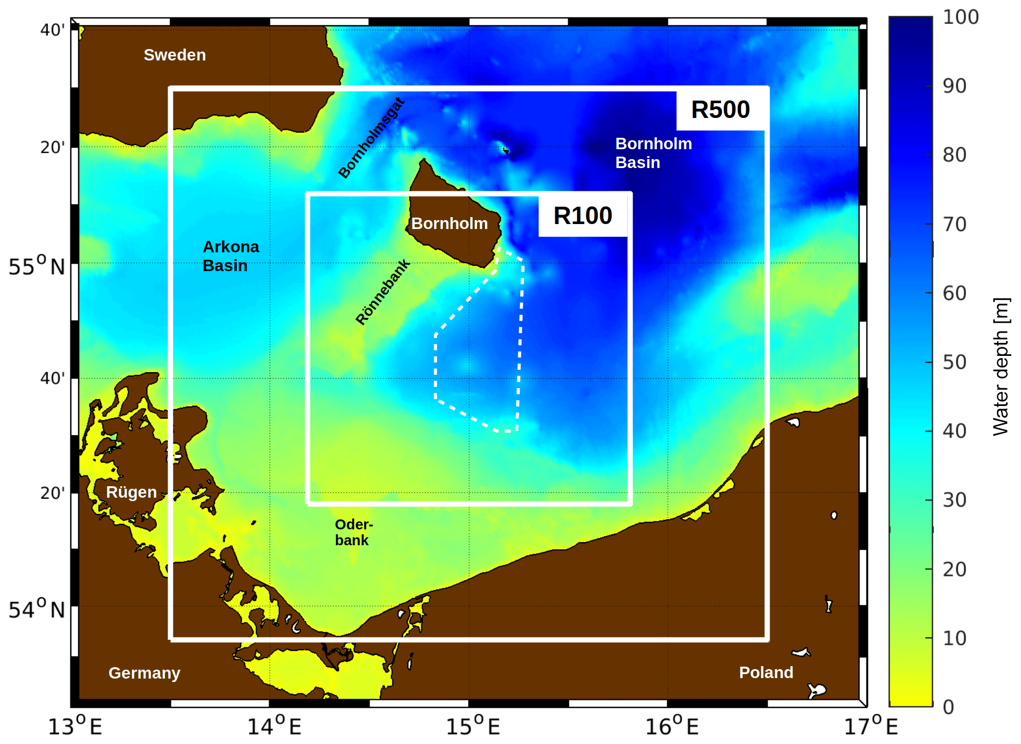
Figure 1The R500 and R100 model domains in the western Baltic Sea. The approximate experimental area of Expedition Clockwork Ocean is indicated by the dashed polygon.
The utilized numerical models are described in Sect. 2. The results of the numerical experiments are presented in Sects. 3 and 4 and compared with observations in Sect. 5, followed by the conclusions. In the following, all time specifications refer to the year 2016 (unless stated otherwise) and are given in UTC (Universal Coordinated Time).
2.1 Geographic and oceanographic setting
The Baltic Sea is a semi-enclosed marginal shelf sea with a mean water depth of 55 m and narrow shallow connections to the North Sea. Due to river runoff, the water balance is positive driving an estuarine circulation with quasi-permanent outflow of fresh surface waters and an intermittent inflow of salty water from the North Sea. At the surface, this creates a horizontal salinity gradient with high salinities in the west and almost freshwater conditions in the far north. Salinity increases with depth, thus stratifying the water column year-round and generating a permanent halocline at about 60 m of depth in the deeper basins. For more details see Feistel et al. (2008), Leppäranta and Myrberg (2009), or Osínski et al. (2010).
The area of this model study is separated into two basins, the Arkona Basin and the Bornholm Basin (Fig. 1). The Arkona Basin is the smaller one, with a maximum water depth of 51 m, while the maximum depth of the Bornholm Basin is 92 m. The basins are connected by two channels, with an exchange of water limited by sills of 45 m depth in the Bornholmsgat (Magaard and Rheinheimer, 1974) and 31 m between Rönnebank and the island of Rügen.
2.2 The CMEMS product
The CMEMS product has been provided at http://marine.copernicus.eu as product BALTICSEA_ANALYSIS_FORECAST_PHY_003_006 (last access 17 February 2020) since April 2015. The product is based on HBM (HIROMB-BOOS model; Berg, 2012), which is an operational ocean circulation model predicting the physical conditions of the Baltic Sea. It is referred to as CMEMS-HBM in the following. CMEMS-HBM used in this study is documented in the product user manual (CMEMS-BAL-PUM-003-006.pdf, version 2.1), and the validation framework is described in the quality information document (CMEMS-BAL-QUID-003-006.pdf). HBM is running twice daily at DMI (Danish Meteorological Institute) in Denmark, and a backup production system is running at BSH (Bundesamt für Seeschifffahrt und Hydrography) in Germany. While the DMI setup uses meteorological data from DMI-HIRLAM with a horizontal resolution of 5 km, the BSH version is driven by data from the Cosmo-EU model with 7 km horizontal resolution provided by the German Weather Service (DWD). CMEMS-HBM comprises daily mean and hourly instantaneous fields at a horizontal resolution of 1 nmi (nautical mile) at 25 depth levels spaced at 5 m between the sea surface and 100 m of depth, with additional levels below at 150, 200, 300, and 400 m of depth. For this article, the daily mean fields of June 2016 were utilized that contained 30 records of the prognostic variables potential temperature, salinity, horizontal velocity, and sea surface height for each June day.
The modelling activity for this study started in early 2017. At that time, the CMEMS-HBM reanalysis product, BALTICSEA_RENALYSIS_PHY_003_011 (also available at http://marine.copernicus.eu), was not yet available since it was released for the first time in April 2018. Hence, there was no alternative for CMEMS-HBM at the required horizontal resolution.
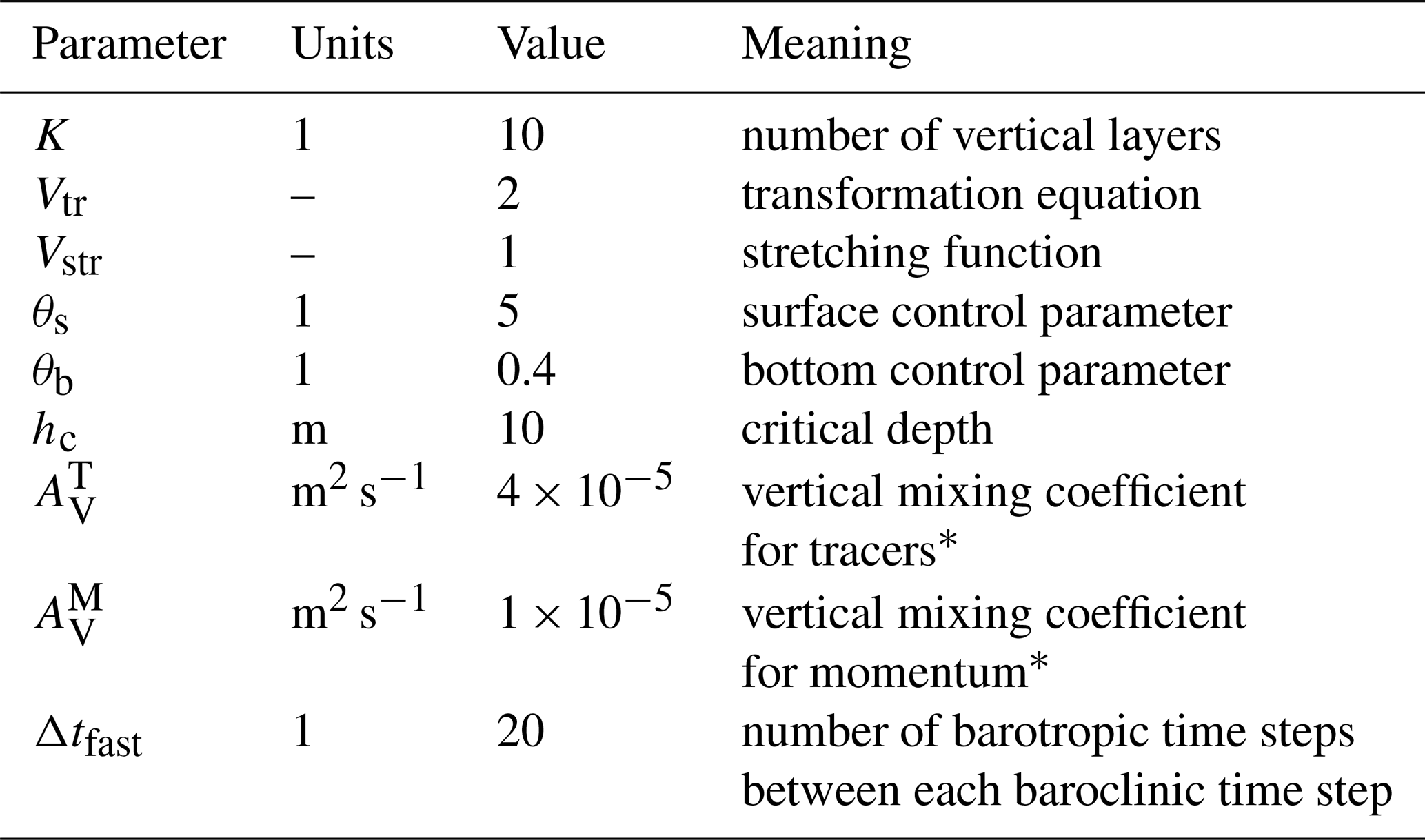
Table 1Parameter settings and the equations used common to all ROMS setups.
2.3 ROMS
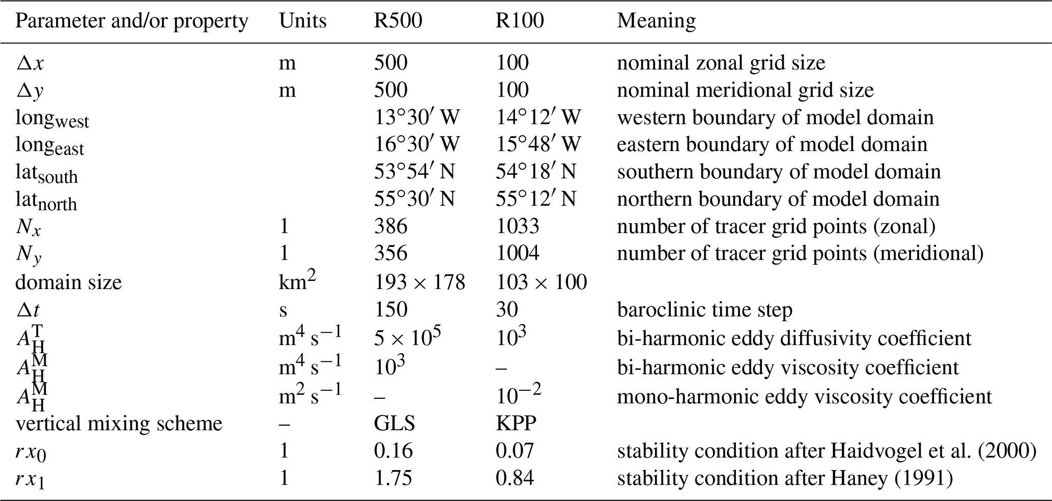
The employed numerical ocean circulation model ROMS is a hydrostatic, free-surface, primitive-equations model. Its algorithms are described in detail in Shchepetkin and McWilliams (2005). In the vertical, the primitive equations are discretized over a variable topography using stretched terrain-following coordinates, so-called s coordinates (Song and Haidvogel, 1994). In the horizontal, spherical coordinates are used. Bi-harmonic mixing along isopycnic surfaces is applied to the tracers in both R500 and R100, while bi-harmonic mixing of momentum is used in R500 and a mono-harmonic formulation in R100. The vertical mixing of momentum and tracers is parameterized with the GLS (generic length scale) scheme by Umlauf and Burchard (2003) in R500 and with the interior closure by Large et al. (1994) in R100, referred to as the KPP scheme. For the bottom friction, a quadratic law is applied, and the pressure gradient term is computed using the standard density Jacobian algorithm by Shchepetkin and Williams (2001). The air–sea interaction boundary layer in ROMS is formulated by means of the bulk parameterization by Fairall et al. (1996). R500 and R100 have the parameters and equations listed in Table 1 in common, while the individual grid-size-dependent parameters and properties are summarized in Table 2. As the spatial scales of the smallest known STPPs are 𝒪(10 m), it is expected that large- and medium-scale STPPs are resolved.
Haidvogel et al. (2000)Haney (1991)Table 2Parameter settings and properties of the R500 and R100 setups.
2.4 Nesting, boundary conditions
There are two offline nesting steps: R500 is nested in CMEMS-HBM, and R100 is nested in R500. While the ROMS-to-ROMS nesting is technically straightforward, the first nest is somewhat more delicate because the CMEMS-HBM output is provided on depth levels, while ROMS uses s coordinates. Therefore, the setup of the R500 domain and the nesting was accomplished as follows.
-
The bathymetry of the GEBCO_2014 grid (General Bathymetric Chart of the Oceans, 30 arcsec horizontal resolution) was used as the lower boundary of the R500 domain, and it was smoothed iteratively until the stability condition rx0≤0.2 was reached everywhere (see Haidvogel et al., 2000, and Table 2).
-
The CMEMS-HBM prognostic variables were interpolated linearly onto the R500 horizontal grid at each CMEMS-HBM depth level in 24 h intervals and for each day of June.
-
The R500 vertical grid was defined according to Table 1, and the CMEMS-HBM fields were interpolated vertically onto the R500 vertical grid. The first record of the resulting data set served as the initial condition for the R500 integration, while the lateral boundary conditions were extracted from all records.
-
R500 was integrated for 1 d, and the near-bottom velocities were checked for odd features that might have been caused by non-zero normal velocities at topographic obstacles which were not resolved in CMEMS-HBM. If such features (e.g. abnormal vertical motions) were noticed, the R500 bathymetry was manually adjusted and the above procedure was iteratively repeated starting with step 3.
For the R500-to-R100 nesting, the same vertical grid definition was used, and no interpolation from depth levels to s coordinates was required. Special care was taken for the preparation of the initial and boundary conditions, as a nesting ratio of 5 is rather challenging: cubic splines were used for the horizontal interpolation of the prognostic variables of R500 onto the child's grid because the structures of jet flows across the open boundaries of the R100 domain looked more realistic than those obtained by linear interpolation. In addition, the downscaled fields were generated in 3 h intervals, leading to a smoother temporal change in the lateral boundary conditions. Cubic splines were used as well for the interpolation of the atmospheric forcing fields on the R100 grid. Because in a nested configuration the s coordinates of the parent and the child at any location are only identical if the bathymetry is the same, the bathymetry of R100 was cloned from R500 and linearly interpolated onto the finer grid.
For each nest, radiation boundary conditions with nudging (Marchesiello et al., 2001) were applied to temperature and salinity, barotropic and baroclinic momentum, and the mixing of turbulent kinetic energy along the lateral boundaries. The boundary conditions of the free surface were defined according to Chapman (1985). In all ROMS setups, the nudging timescales were set to 2 d for the corresponding variables. At the surface, the air–sea interaction in the ROMS nests was specified by means of atmospheric forcing fields from the so-called “assimilation runs” of the ICON-EU model provided by the German Weather Service (DWD). The output of these runs was considered to be the best available product because the runs were initialized in 3 h intervals at 00:00, 03:00, and 06:00 h (and so on) and driven by the most recent near-real-time assimilation fields in contrast to the forecast runs initialized semi-daily at 00:00 and 12:00. The horizontal resolution of ICON-EU is about 6.5 km, and output is produced in 1 h intervals.
STPPs are generated in the straining field of mesoscale eddies. According to Osínski et al. (2010), the condition for eddy-resolving models of the southern Baltic is that the Rossby radius is resolved by at least four to five horizontal nodes. As the Rossby radii in the Bornholm and Arkona basins are in summer around 7.2 and 3.7 km, respectively (Fennel et al., 1991), and since the grid size of CMEMS-HBM is 1 nmi, it is definitively not eddy-resolving or even eddy-permitting (two to three nodes) in the Arkona Basin and perhaps eddy-permitting at best in the Bornholm Basin. The eddy-resolving R500 was initialized from CMEMS-HBM on 1 June at 00:00 and integrated for 30 d. The vertical mixing in R500 is accomplished with GLS using the k−ω setup of Wilcox (1988) with the stability function of Kantha and Clayson (1994).
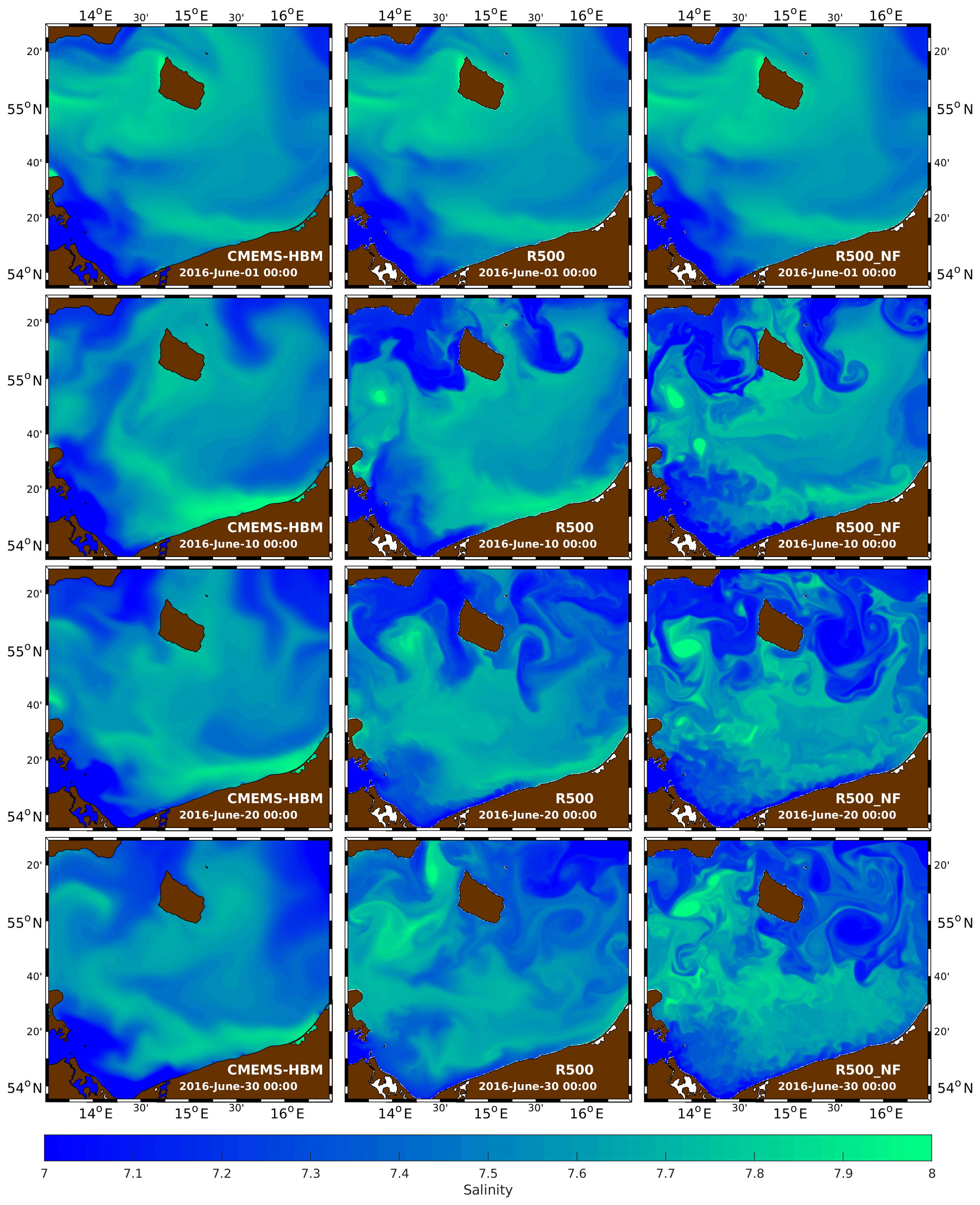
Figure 2Top-layer salinity in CMEMS-HBM (left column), R500 (centre), and R500_NF (right) for 1, 10, 20, and 30 June. The CMEMS-HBM fields are interpolated onto the R500 horizontal grid. Due to the coarser horizontal grid of CMEMS-HBM, inland lakes are not resolved, and salinity values were assigned to places that are dry in R500.
For a Lagrangian water parcel, the freshwater budget is controlled by P–E, which is the difference between precipitation P and evaporation E. On long-term average, P–E is around 0.1 mm d−1 (Smedman et al., 2005), which may cause maximum salinity changes on the order of 10−2 per month for typical mixed-layer depths of 10 m (see Sect. 4.4.3). In contrast, the heat budget is dominated by the shortwave radiation flux, leading to warming of around 5 ∘C of the near-surface layers in June. Hence, salinity is the ideal parameter to trace turbulent patterns, as in the Baltic Sea it behaves like a passive and quasi-conservative tracer. Figure 2 shows salinity in the uppermost layer of CMEMS-HBM and R500 on 1, 10, 20, and 30 June (left and centre panels). R500 rapidly develops turbulent structures that are only marginally identifiable in CMEMS-HBM. These are, for example, the low-salinity outbreaks along the northern boundary, a high-salinity eddy in the Arkona Basin, and mushroom-like patterns east and southeast of Bornholm on 10 and 20 June. The horizontal scales of these features are 𝒪(10 nmi), but smaller patterns with a horizontal extent of 5 nmi, or even less, are also generated by R500, such as the filaments around Bornholm and the meanders immediately off the Polish coast on 20 June. Hence, R500 apparently bridges the gap between the mesoscale and the submesoscale.
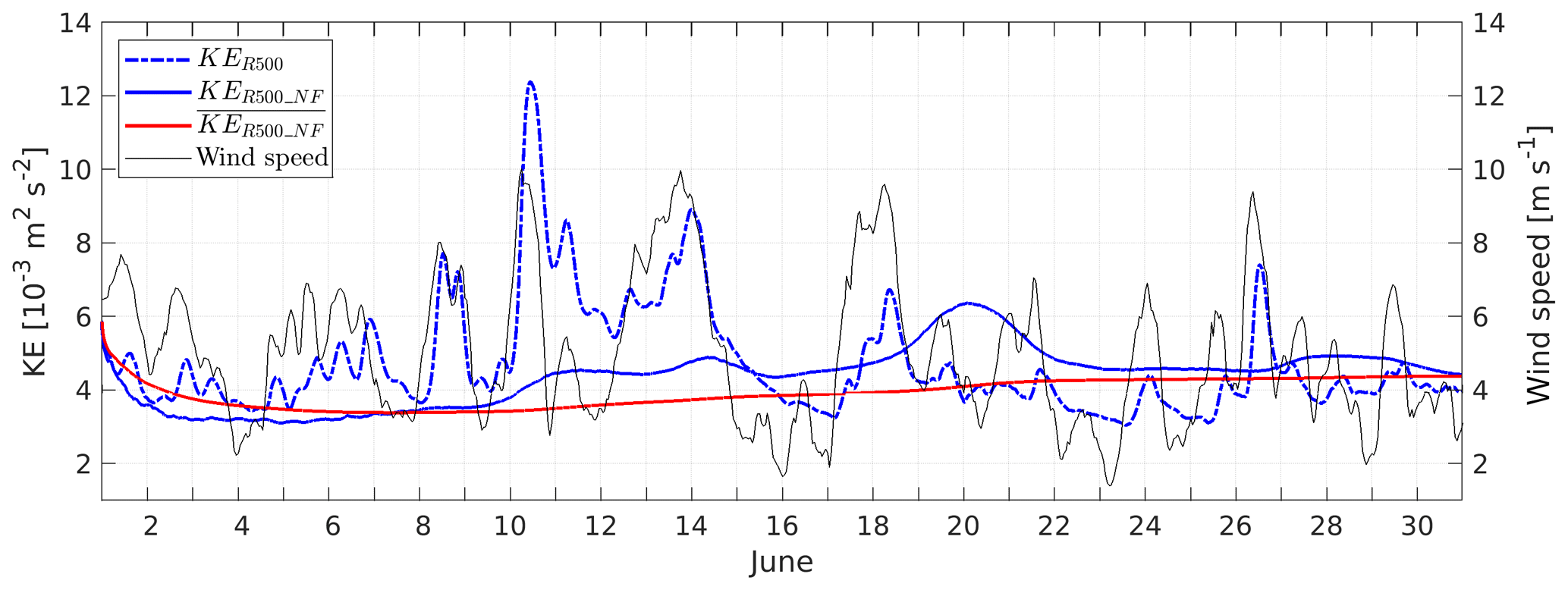
Figure 3Instantaneous (KER500, KER500_NF) and cumulatively averaged () kinetic energy per unit mass of the model runs R500 and R500_NF. The wind speed is shown as a black curve. All quantities are averaged over the model domain.
R500 provides the initial and boundary conditions for R100. It is worth knowing to what extent its generated two-dimensional turbulence is in a state of statistical equilibrium and at what time during the integration an equilibrium state is attained. To determine this so-called spin-up time, the blue dash-dotted graph in Fig. 3 shows a time series of the domain-averaged kinetic energy per unit mass, KER500; it fluctuates strongly between and more than m2 s−2 and does not reach a stable value. Evidently, it is difficult to determine the spin-up time from R500 because KER500 is strongly impacted by wind bursts as shown by the black curve. Therefore, R500 was compared to a run in which the atmospheric forcing was completely turned off by setting the air–sea fluxes of net heat, fresh water, and momentum to zero. This run is referred to as R500_NF (“no forcing”). Here, the intense fluctuations of KE vanished as shown by KER500_NF (blue solid graph), but there are still some smaller-scale oscillations with maxima on 11, 14, 20, and 28 June, the existence of which impedes the estimate of a spin-up time. These oscillations are slightly correlated with the wind bursts lagging behind for about 1 d. Potentially, they are triggered by the remote forcing of CMEMS-HBM via the lateral boundaries, which explains the time lag. Another cause could be vacillations of KE, which is a well-known peculiarity of nonlinear rotating fluids (Hide, 1958; Früh, 2015). In order to filter out the oscillations, the cumulative average was computed. This quantity is frequently used in time series analysis in order to determine the timescale at which a stochastic time series reaches stationarity. In the actual case, attains a maximum of on 1 June and then decreases to about m2 s−2 on 7 June. Thereafter, it increases steadily to on 22 June and remains constant until the end of the month. Hence, stationarity is reached after about 22 d, corresponding to an e-folding scale of 12 d that may be considered the spin-up time.
The analysis of the prognostic fields of R500_NF yielded an additional perception: the tracer fields exhibit much more spatial variability in comparison to the corresponding fields of R500 (see the right panels in Fig. 2). A rich variety of smaller details is revealed that were hidden in the forced run, such as the STPPs along the German and Polish coast, multiple filaments in the entire model domain, and sharper frontal gradients. On longer timescales, the larger-scale patterns also develop differently. Similar findings were presented by the observational study of Kubryakov and Stanichny (2015): from an analysis of satellite altimeter data, they demonstrated that a weakening of the large-scale circulation leads to baroclinic instability of the Rim Current in the Black Sea. An explanation for this behaviour was provided by the earlier studies of Zatsepin et al. (2005). Literally, their laboratory experiments showed that “the development of an instability, the generation of meanders, and the formation of eddies are prevented by the Ekman divergent circulation caused by the wind, which presses the frontal current to the coast throughout the periphery of the tank, thus contributing to the significant increase in kinetic and available potential energy. When the wind forcing stops, the instability grows rapidly.” While the above-mentioned papers focused on mesoscale instabilities, Renault et al. (2018) showed that the evolution of submesoscale instabilities in the California upwelling system is damped by the wind stress as well. Another reason for the decrease in submesoscale activity in response to the increase in the wind speed was provided by Mahadevan et al. (2010), who showed that the wind field blurs the small-scale features by horizontal mixing. These findings are important because they guide the setup of the R100 experiments below.
A comparison with observations is shown in Fig. 4 by means of the surface salinity from R500 and a red–green–blue (RGB) composite derived from a satellite-borne multi-spectral image in the visible spectral range. In the latter, the patterns arise due to the presence of naturally occurring optically active substances like chlorophyll. The comparison between these different quantities is legitimate because both act like passive flow tracers. The image reveals three spiral-like patterns that may be considered proxies for cyclonic (C1, C2) and anticyclonic (AC) eddies. The centre of C1 is almost at exactly the same location (15∘30′ E, 54∘40′ N) in the satellite image and in R500. The centre of C2 is at about 14∘10′ E, 55∘7′ N in R500. Unfortunately, the central part of this cyclone is masked by clouds in the satellite image, but the unmasked portions provide evidence for its existence. Strong peripheral fronts are visible in both R500 and the satellite images. The positions of AC differ the most: in Fig. 4b, the centre of that anticyclone is at 15∘50′ E, 54∘57′ N, and in Fig. 4a it is at about 15∘40′ E, 55∘0′ N, hence roughly 7 nmi to the west. It is legitimate to associate these positions with each other because in both R500 and in the satellite snapshot, as AC is the anticyclonic “partner” of C1, both form a mushroom-like eddy pair. On the whole, the apparent similarities between the observations and the R500 simulations builds some confidence that R500 produces realistic results. Moreover, the above-mentioned eddies and fronts are already visible on 20 June in R500 (see Fig. 2) but not at all in CMEMS-HBM at the same time. Hence, in R500 the mesoscale environment is apparently better reproduced than in CMEMS-HBM.
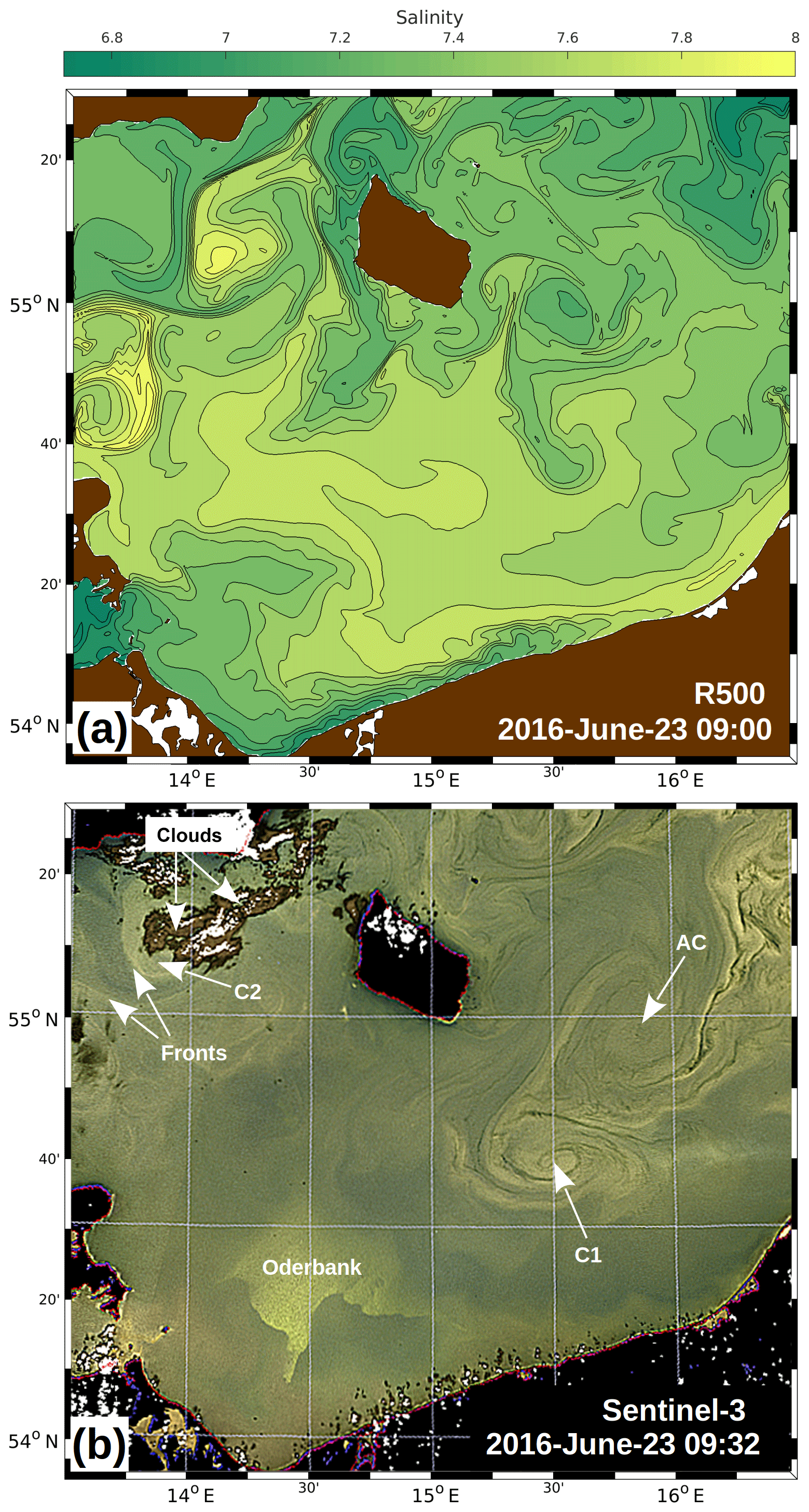
Figure 4(a) Top-layer salinity of the R500 model on 23 June at 09:00. (b) RGB composite from the Ocean and Land Colour Instrument of ESA satellite Sentinel-3 for the R500 domain on 23 June at 09:32. The original image was manually adjusted in order to fit the Mercator projection used in (a). C1, C2, and AC refer to the signatures of cyclonic and anticyclonic eddies, respectively. For the Oderbank; see Fig. 1.
Apparently, R500 is able to reproduce STPPs but only those in the low-wavenumber part of the spectrum. To provide more insight into the higher-wavenumber parts, R100 was initialized from R500 on 15 June at 00:00 and integrated until 29 June at 00:00. Based on the experience with R500, the surface fluxes in R100 were turned off. This is indeed a strong simplification and the model results may differ significantly from the reality. However, it helps to understand the evolution and the dynamics of submesoscale processes, which are controlled primarily by potential vorticity conservation in the adiabatic limit (McWilliams, 2008). Different formulations and coefficients for the horizontal eddy viscosity and diffusivity were tested. The best results were obtained from a model run with mono-harmonic mixing for the momentum and bi-harmonic mixing for the tracers (Table 2). This choice caused a minimum damping of STPPs and a better representation of small-scale details without numerical noise. Moreover, the vertical mixing was parameterized with KPP instead of the time-consuming GLS scheme. From a KE analysis, the spin-up time was an estimated 2 d. Hence, a 6 d spin-up period starting on 15 June was sufficient to produce statistically equilibrated fields on 20 June and thereafter.
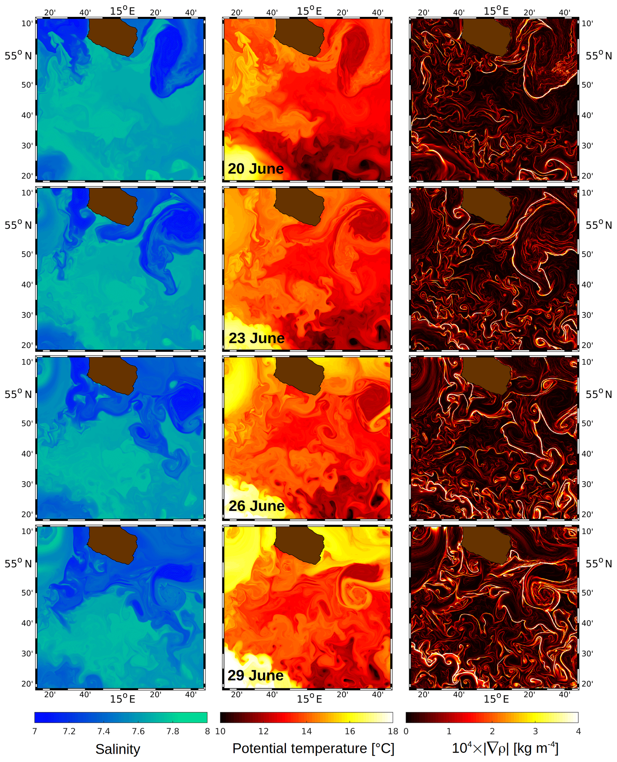
Figure 5R100: top-layer salinity (left column), potential temperature (centre), and the absolute horizontal gradient of potential density (right) on 20, 23, 26, and 29 June. The upper end of the colour axis of is limited to kg m−4 to distinguish higher gradients from the dark background.
In the following, the results of R100 are illustrated by Figs. 5–17 and 18b and c. All figures are snapshots taken on the specified day at 00:00.
4.1 Tracer patterns
The top-layer patterns of salinity and potential temperature are shown in the left and centre panels of Fig. 5 in 3 d intervals for 20–29 June, where the top layer ranges between about 0.3 and 1.7 m. To assess the effect of the downscaling, the salinity patterns are compared with the corresponding ones of R500_NF on 20 and 30 June (Fig. 2). The large-scale features resemble each other to a high degree, such as the low salinity to the west and the east of Bornholm and the higher-salinity pool south of the island. However, R100 exhibits much more variability in the submesoscale waveband, and STPPs down to 1 km scales are resolved. The signatures of such small-scale features are better visible in the temperature patterns, such as the cold patches in the southern region of the R100 domain.
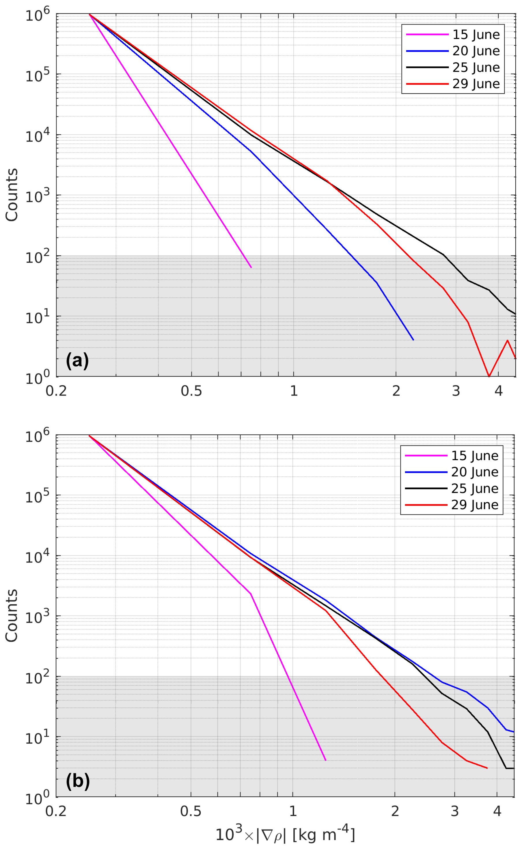
Figure 6R100: frequency distribution of in the top layer. The initial and open boundary conditions for R100 were provided by (a) R500 and (b) R500_NF, respectively. The values were binned in 10 intervals of kg m−4 width between 0 and kg m−4. Counts <100 (gray shaded) representing less than 0.1 % of the total number of horizontal grid points were not considered significant.
Knowledge of the temporal change in the density (or buoyancy) gradient is essential for frontogenetic and frontolytic processes and filamentogenesis, which is expressed by the frontal tendency equation (Holton, 1982; Capet et al., 2008b; Gula et al., 2014). As a first approach, the absolute horizontal gradient of potential density, ρ,
is calculated, where x and y are the Cartesian coordinates pointing to the east and to the north, respectively. This quantity is shown in the right column of Fig. 5. Narrow filaments indicate locations of intensified gradients, i.e. density fronts. From the sequence of the images, it appears that the quantity of the fronts increases with time and that the gradients amplify. This is partly confirmed by a frequency distribution of , shown in Fig. 6a: from 15 to 25 June, the frequency of occurrence grows consistently in all intervals. From 25 to 29 June, however, this behaviour changes. While the frequency distribution for kg m−4 remains almost the same, it decays at the same time for larger values of . Hence, there are fewer locations with strong gradients, indicating a weakening of strong density fronts. In order to determine whether there is an upper limit for the growth of , R100 was repeated but with the initial and open boundary conditions taken from R500_NF. The resulting frequency distribution (Fig. 6b) exhibits more occurrences of strong gradients than in panel (a) on 15 and 20 June. This is plausible because the atmospheric forcing in R500 has blurred the gradients. The frequency distribution of 25 June is almost identical to that of 20 June, and from 25 to 29 June it decays in the same way as in panel (a). Hence, a “frontal arrest” apparently occurs when the strongest gradients approach a critical value around kg m−4, which is reached on 25 June in panel (a) and on 20 June in panel (b). However, it is not clear whether physical processes or numerical diffusion (or both) limit the increase in gradients. For the physical processes, Qw, the straining deformation by the vertical velocity (see Eq. 7) would be a suitable candidate because downwelling on the dense side of a front and upwelling on the less dense side lead to a weakening of the cross-front density contrast. Another process was identified by Sullivan and McWilliams (2018) and Gula et al. (2014), who investigated the life cycle of a dense filament. Therein, frontogenesis is arrested at a small width of about 100 m. It is mostly driven by an enhancement of turbulence through submesoscale horizontal shear instabilities that draw their energy primarily from the horizontal mean shear via the horizontal Reynolds stresses.

Figure 7R100, 26 June: (a) magnitude and direction of top-layer horizontal velocity V (vectors are plotted at 3 km resolution), (b) relative vorticity ζ and (c) horizontal divergence δ, each scaled by f, (d) vertical velocity w at 5 m of depth. The white line in (a) is the 40 m depth contour. The blue box in (a) refers to the zoomed area shown in Figs. 11 and 12, the box in (c) is the zoomed area of Fig. 8, and the box in (d) is the zoom shown in Fig. 15.
4.2 Kinematics
Figure 7 shows the near-surface properties of the velocity field and derived quantities on 26 June. This day was chosen because it represents the conditions in the middle of the survey period and allows for comparisons with Fig. 5.
4.2.1 Horizontal currents
The horizontal velocity field (Fig. 7a) is separated into two regimes: high current speeds frequently exceeding 0.1 m s−1 are found north of about 54∘50′ N, south of 54∘35′ N, and west of 14∘40′ E. They are organized in jet-like streaks or circular features, and their positions are clearly related to the main density fronts shown in Fig. 5. Maximum speeds of 0.32 m s−1 are found in the anticyclonic eddy southeast of Bornholm. The high-speed regime surrounds a pool of water with speeds lower than 0.1 m s−1 in the centre of the model domain. The transition between the high-speed and low-speed regimes appears to be related to the 40 m depth contour (the white line in Fig. 7a), at least in the south and west. Potentially, the bathymetry acts as a waveguide for the westward jet south of Bornholm. One may note that both the anticyclone (AC) and the cyclonic eddy C1 are at about the same position as in Fig. 4a 3 d before.
4.2.2 Relative vorticity
Information about the dynamical properties of the flow field is derived from the relative vorticity ζ, i.e. the vertical component of the curl of the total velocity:
Here, z is the vertical coordinate, and u, v, and w are the zonal, meridional, and vertical components of the total velocity vector V. Figure 7b reveals the whole range of relative vorticity (scaled by f) between the largest scales of about 20 km and the smallest scales on the order of the grid size of 100 m. The dominant mesoscale patterns are the large anticyclonic relative vorticity patch southeast of Bornholm and the wave-like structures to the south that belong to the westward jet mentioned above. Further west and south in the shallow water, pools of concentrated cyclonic relative vorticity vary mostly between 5 and <1 km in size. The smallest visible features are cyclonic streamers, with a width approaching the Nyquist scale of 200 m.
There is a strong asymmetry between the distributions of cyclonic and anticyclonic relative vorticity. The cyclonic relative vorticity is organized in thin filaments, comma-like “hooks”, and quasi-circular pools of water. In contrast, the distribution of the anticyclonic relative vorticity is smoother, and the occupied area is larger than the area utilized by , which is in agreement with McWilliams (2016). The frequency distribution shows that in 63 % of the grid cells, while positive values are found only in 37 %. Moreover, in less than 0.2 % of the grid cells, , indicating negative potential vorticity (Dewar et al., 2015; Gula et al., 2016b) and associated inertial instability.
The relative vorticity structures north of 55∘ N exhibit lamellar patterns that are probably caused by false advection from the parent domain, although cubic splines were applied to all prognostic variables in the context of the downscaling. Such patterns are only visible in the relative vorticity patterns, while the horizontal velocities (Fig. 7a) and the tracer fields (Fig. 5) look rather reliable. Obviously, the downscaling did a good job with the prognostic variables, but along the open boundaries it may not have been able to reflect the first derivatives correctly.
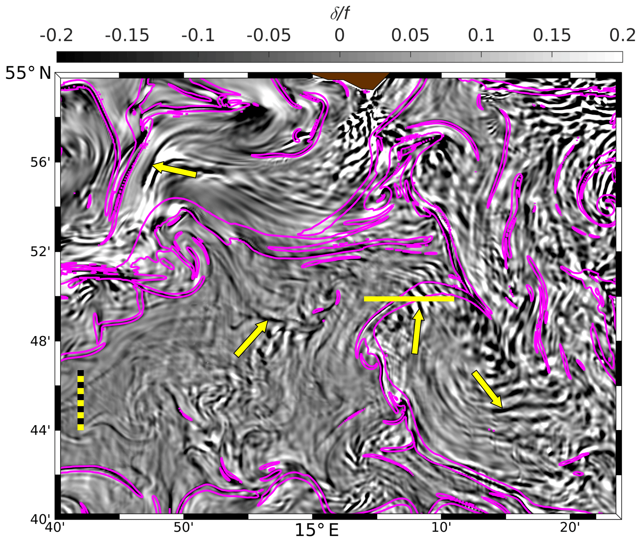
Figure 8R100, 26 June: zoom of f-scaled horizontal divergence δ (grayscale image; for the position of the zoomed area see Fig. 7c). Bright areas indicate divergent flow, and convergences appear dark. The magenta lines show the kg m−4 contours. The yellow arrows likely mark internal wave packages as discussed in the text. The horizontal yellow line is the position of the section shown in Fig. 9. The dashed ruler represents a distance of 5 km.

4.2.3 Divergence and vertical motion, impact of bathymetry
The horizontal divergence of the velocity,
is displayed in Fig. 7c. It can be divided into three different classes of textures: Class I structures are thin, less than 1 km wide filaments of negative divergence (convergent flow) that are bordered by wider areas of divergent flow on one or both sides. The major density fronts (Fig. 8) are aligned with such filaments. In contrast, the areas of convergent flow that are not congruent with enhanced horizontal density gradients belong to Class II. In particular, those patterns tagged by the yellow arrows in Fig. 8 are not correlated with enhanced density gradients (note that the value in magenta already refers to rather low gradients; see Fig. 5). It is conjectured that these features are related to internal waves generated during the genesis of nearby fronts and jets (Plougonven and Snyder, 2007; Shakespeare and Taylor, 2014; Shakespeare, 2019). This is confirmed by Fig. 9: the vertical displacements of isopycnals between E and E are clear indicators for internal waves with a wavelength around 1000 m. In order to verify that these patterns are caused by internal waves, their frequency at 10 m of depth was estimated to about s−1, somewhat less than the buoyancy frequency at the same depth ( s−1) but larger than the Coriolis frequency. Hence, the patterns are indeed intermediate-frequency internal waves. However, a closer inspection is not advisable because ROMS is hydrostatic, and various properties of internal waves are correctly reproduced only in nonhydrostatic models (Wadzuk and Hodges, 2009; Vitousek and Fringer, 2011).
Class III textures are small patches of either sign and horizontal scales of 𝒪(1) km. They are found almost everywhere, but their highest values are found in the area of higher current speeds in the northwest corner of the domain and in the anticyclonic eddy southeast of Bornholm. The topography of potential density surfaces in the anticyclone shows that the patches are accompanied by large excursions of isopycnals, indicating intense internal wave activity. These waves are emitted from fronts at the periphery of the eddy, and the superposition of internal waves coming from different directions leads to the rugged shape of isopycnals and contemporaneously to the patchy pattern that is in agreement with the findings of Väli et al. (2018).
In ROMS, the vertical speed is computed from the continuity equation. As expected, the spatial patterns of the vertical speed are therefore identical to that of the divergence but only for the divergence in the top layer and the vertical speed at the base of that layer. In contrast, the horizontal distribution of the vertical speed at 5 m of depth (Fig. 7d) still resembles the top-layer divergence but with significant differences. The most striking discrepancy is that the thin filaments of convergent flow belonging to Class I (Fig. 7c) are not at all reflected by the vertical motion pattern. On the other hand, the vertical motions related to the internal wave packets discussed above are still clearly visible. To explain this disagreement, Fig. 9 shows a zonal section of the vertical speed, together with the potential density and the meridional velocity. The vertical motion induced by the internal waves attains speeds of up to ±20 m d−1 (≈0.2 mm s−1), and the signal is pronounced over the entire vertical range between the surface and 10 m of depth; by contrast, the magnitude at the location of the front barely exceeds 5 m d−1 (≈0.06 mm s−1), and the vertical speed diminishes with increasing depth. Apparently, the major surplus (deficit) of mass created by the frontal convergence (divergence) at the surface is discharged (imported) by the frontal jet or the secondary divergent circulation (see Fig. 1 in McWilliams et al., 2009, or Bleck et al., 1988). As such a horizontal discharge or import mechanism is not available in a pure internal wave field, the only way to respond to any non-zero divergences is by vertical motion; this is explained in more detail in Sect. 4.4.4. In contrast to these rather moderate vertical velocities, extreme values of around ±250 m d−1 (equivalent to ≈3 mm s−1) are associated with the above-mentioned Class III textures.
In Sect. 4.2.1, it was already mentioned that the horizontal current patterns are somehow correlated with the water depth. Such a relationship applies as well for the patterns of the other variables displayed in Fig. 7; e.g. the spatial variability of relative vorticity and the frequency of narrow filaments of confluent flow are clearly enhanced in the shallow water regions. An explanation for this different behaviour is given by McWilliams (2019), who identified two principal mechanisms for the generation of STPPs: (i) extraction of available potential energy due to horizontal gradients in the weakly stratified surface layer (mixed-layer instability) and (ii) topographic-drag vorticity generation in flows along a sloping bottom, followed by boundary current separation and wake instability. As strong bottom slopes are found only along Rönnebank and in the south of the R100 domain (see Fig. 1), the mechanism (ii) is obviously significant in those areas. However, for water depths >50 m, the bottom is mostly flat and topographic-drag vorticity generation can be excluded.
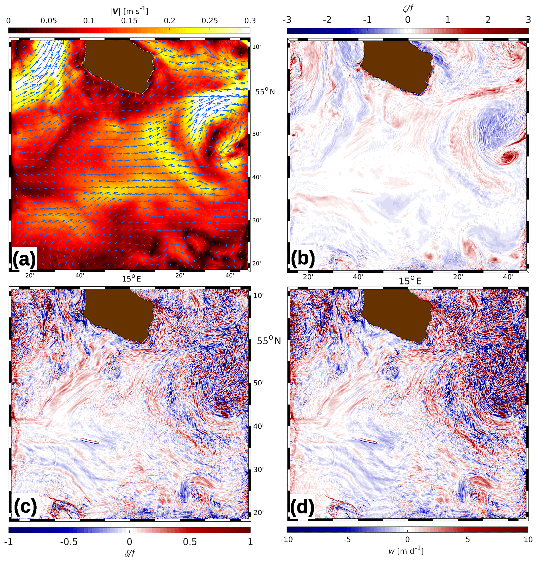
Figure 10R100 with full atmospheric forcing on 26 June: (a) magnitude and direction of top-layer horizontal velocity V (vectors are plotted at 3 km resolution), (b) relative vorticity ζ and (c) horizontal divergence δ, each scaled by f, (d) vertical velocity w at 5 m of depth. For all subplots, the same colour scaling was used as in Fig. 7.
4.3 Impact of atmospheric forcing
In order to justify the approach to run R100 without atmospheric forcing, R100 was repeated but now including all fluxes at the air–sea interface as provided by the ICON-EU model. The results for 26 June for the same parameters as in Fig. 7 are displayed in Fig. 10.
The patterns of the horizontal velocity (Figs. 7a and 10a) resemble each other but only in the “high-velocity regimes” west and east of Bornholm. Here, the direction of the currents did not change significantly, but the maximum speeds increased from 0.32 to about 0.42 ms−1. In contrast, the pattern in the low-speed pool in the centre of the model domain changed dramatically. While in the no-forcing run the maximum speeds rarely exceeded 0.1 ms−1, the highest speeds are now about twice as high. Moreover, the wind stress caused a unidirectional flow to the east as opposed to the alternating flow directions in Fig. 7a. The atmospheric forcing severely impacts the top-layer relative vorticity patterns (panels b of the respective figures). Submesoscale features are no longer detectable; i.e. there are no filaments, comma-like hooks, and circular pools of cyclonic vorticity. However, some mesoscale structures are still visible, for instance the large anticyclonic eddy southeast of Bornholm and the small cyclone close to the eastern boundary at about 54∘45′ N. Overall, the atmospheric forcing acts like a filter that wiped out any structures with scales of less than about 10 km. This smoothing effect also removed the Class I divergence patterns (panels c). In contrast, the number of small-scale patches (Class III) and their amplitudes have increased. This is also reflected by the vertical velocity (panels d). Presumably, the imposed momentum stress enhanced the internal wave activity.
In summary, STTPs only start to grow after the atmospheric forcing is switched off. This reflects a situation which also occurs in nature when the wind subsides. For instance, applying a high-resolution Princeton ocean model to the Gulf of Finland, Zhurbas et al. (2008) and Väli et al. (2017) demonstrated that the horizontal eddy viscosity increased and submesoscale cyclonic vortices evolved as soon as the wind slackened.
4.4 Fronts and eddies
4.4.1 Frontogenesis and eddy formation
The right column of Fig. 5 shows snapshots of . A statistical analysis indicates an increase in the frequency of occurrence of high-density gradients and a general sharpening of the density fronts with time. However, the latter provides only statistical information; it does not show the locations where the fronts are sharpening (frontogenesis) or weakening (frontolysis) and which physical processes are contributing thereto. The missing information is conveyed by the frontal tendency equation
which was introduced by Hoskins (1982) into the meteorological literature. F describes whether the absolute horizontal density gradient of a Lagrangian water parcel is growing (F>0) or weakening (F<0) with time t. Using the nomenclature of Capet et al. (2008b), F is further decomposed as
Here, the terms are defined as
which is the vector representing the straining deformation by the horizontal total velocity. The vector may be separated into contributions Qgeo from the geostrophic and Qageo from the ageostrophic velocity, respectively.
is the equivalent quantity for the vertical velocity, and
is the contribution from vertical mixing, where is the eddy diffusion coefficient for density. Finally,
is the effect of the horizontal diffusion of density, D.

Figure 11R100: near-surface properties on 26 June within the blue box depicted in Fig. 7a. (a) Absolute horizontal density gradient (10−4 kg m−4) and (b) scaled relative vorticity ζ∕f in the top layer, (c) vertical velocity w (m d−1) at the base of the top layer. (d)–(i) The frontal tendency F and the components of the tendency equation Qgeo, Qageo, Qw, Qdv, and Qdh (10−13 kg−2 m−8 s−1) at 2 m of depth. Red marks frontogenesis, and blue marks frontolysis. For the labels F1–F4, C3, and C4, see the text. The dashed rulers represent a distance of 2 km; vectors in (e) and (f) are drawn at 600 m intervals.
The components of the tendency equation are displayed in Fig. 11 for a subregion of the R100 domain. The quantities F, Qgeo, Qageo, Qw, Qdv, and Qdh at 2 m of depth are shown in the centre and bottom rows. They are the scalar products of the corresponding vectorial quantities Q and ∇ρ. For comparison with the dynamical background, the top-layer patterns of and ζ∕f, as well as the vertical velocity w at the base of the top layer, are displayed in the top row of the same figure. The subplots of and ζ∕f reveal four major frontal systems, F1–F4, and two cyclonic vortices, C3 and C4. The width of all fronts and the radius of the circular cyclone C3 (defined by the zero crossings of ζ∕f) are ≤2 km, while the semi-axes of the elliptically shaped cyclone C4 vary between 2 km and about 4 km. Both frontogenetic and frontolytic processes are roughly evenly distributed and of the same order of magnitude for F, Qgeo, and Qw. This is different for Qageo and Qdv which are primarily frontogenetic. Moreover, Qdv only differs significantly from zero at the fronts, while at the positions of C3 and C4 it is close to zero. By contrast, the contribution of Qdh to the tendency F is negligible everywhere. F exhibits a bimodal pattern for F1 and F2, with F<0 on the anticyclonically sheared side and F>0 on the cyclonic side. A comparison of the patterns of the components of F reveals that F>0 in F1 and in the western and central parts of F2 is predominantly supported by Qageo, Qdv, and to a lesser extent by Qgeo, while the sign of Qw alternates along-front. On the other hand, F<0 in those parts is primarily supported both by Qgeo<0 and Qdv<0. A bimodal structure is also visible for F4. Here, frontogenesis is supported by both Qgeo and Qageo, and frontolysis is only supported by Qw. For F3, the situation is similar.
The above results conflict with those obtained by Capet et al. (2008b), referred to as CMMS in the following: according to their Fig. 7, the “residual” (equivalent to F in this paper) at the sea surface is generally negative and the geostrophic contribution is always positive, while the corresponding quantities in the current article exhibit a clear bimodal structure. On the other hand, the contributions from ageostrophic straining and vertical diffusion are bimodal in CMMS, but Qageo and Qdv are predominantly positive. Similarly, the impact from vertical straining in CMMS is negative everywhere in contrast to Qw, which is bimodal as well, and with the sign alternating along-front. The cause for these disagreements might be the different horizontal resolution of ROMS (750 m in CMMS and 100 m in R100). By contrast, the multimodal structures and the alternating along-front sign changes of F and its components more closely resemble those obtained by Gula et al. (2014).
Prominent structures of the tendency terms are also visible in C3 and C4, but those will be investigated in detail in a follow-up paper investigating the dynamics of a submesoscale cyclone.
4.4.2 Submesoscale upwelling in eddies
As noticed above, the vertical motion pattern in almost the entire model domain is impacted by internal waves that frequently blur the corresponding signals of fronts. However, in some settings, the vertical motion related to submesoscale fronts and eddies may supersede the internal wave-driven vertical velocity, which can be seen in Fig. 7d. Such a situation is given during the life cycle of the submesoscale eddy C3 depicted in Fig. 11. C3 originates from a dense (cold and salty) streamer that invaded the area from the south starting on 24 June around noon. While the streamer stretched farther to the north, it rolled up into C3 on 25 and 26 June (Fig. 12a–c). In Fig. 12d–f, the vertical speed at 5 m of depth is shown for the same period of time. On 24 June before the winding-up of the eddy started, the vertical motion pattern was controlled by a train of internal waves travelling from northeast to southwest. The impact of the eddy formation on the vertical motion field becomes visible 1 d later: two extended patches with vertical speeds of either sign are located south and north of the eddy core. On 26 June, the pronounced downwelling area is smaller but the upwelling still prevails at the same location. Apparently, the eddy-driven vertical motion supersedes the signal of the internal waves and causes persistent upwelling for a day or even more as can be seen in Fig. 12f: at the position of the cross hairs, upwelling is still visible, although the eddy centre has already moved to the north by about 2 nmi. Both the roll-up process and the corresponding vertical velocity are shown in the animation of Onken et al. (2020).
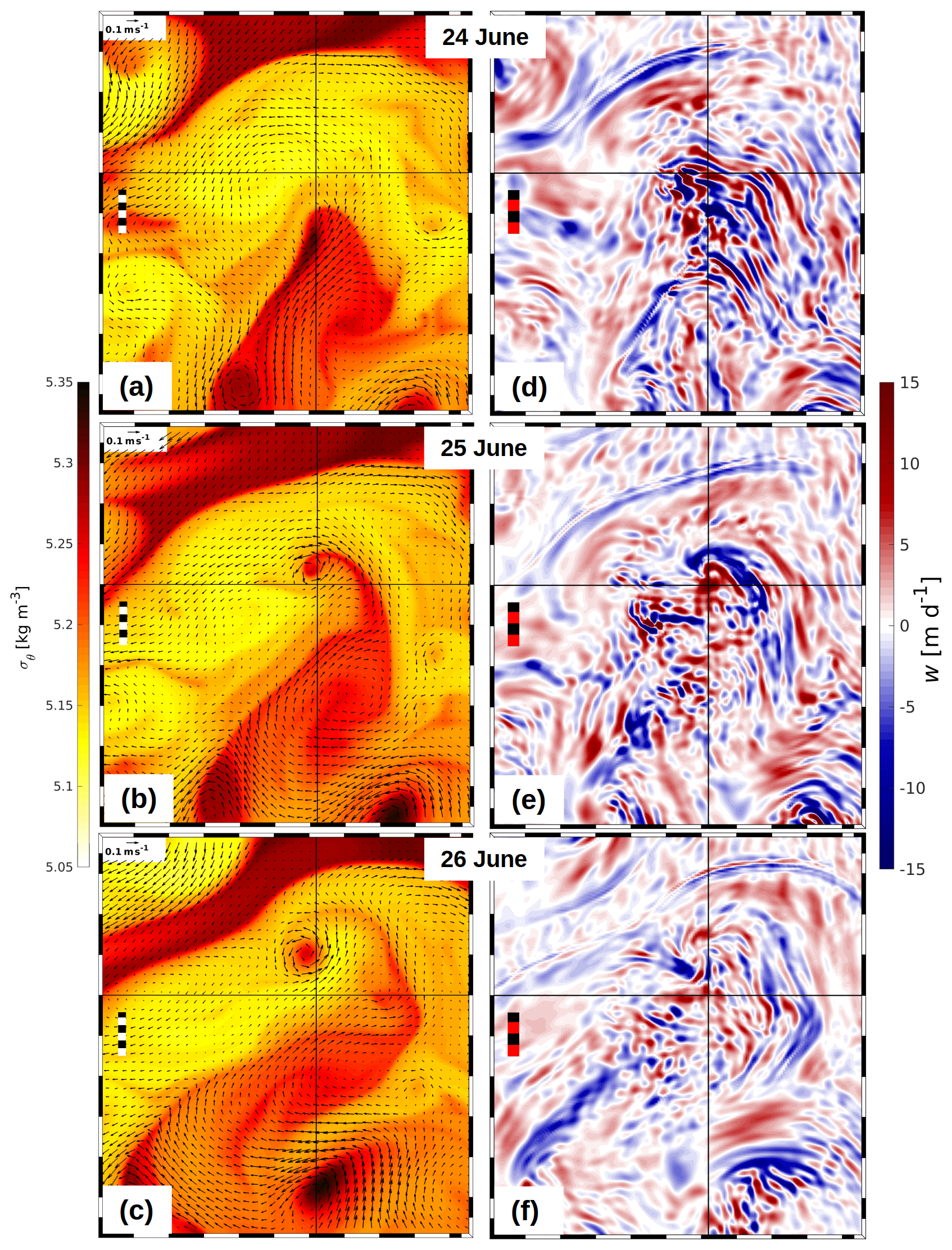
Figure 12 R100: (a)–(c) temporal evolution of a potential density anomaly σθ in the top layer with vectors of total velocity V drawn at 400 m resolution and (d)–(f) corresponding vertical velocity w at 5 m of depth; upwelling is positive. The area shown is indicated by the blue box in Fig. 7a. The cross hairs tag the same position in all subplots.The dashed rulers represent a distance of 2 km.
4.4.3 Instability mechanisms
The results above impressively show that submesoscale eddies grow rapidly in the R100 domain, preferably in the shallow areas with water depths less than 40 m (Fig. 7). However, it is not yet clear if inertial, symmetric, or mixed-layer instability drives the eddy growth. In the following, the R100 fields are analysed for criteria necessary for the occurrence of any type of instability.
For inertial instability, negative absolute vorticity, ζa, is a necessary condition, which is equivalent to or . It can be seen in Fig. 7b (blue regions) that is satisfied along the coast of Bornholm and at a few isolated locations along the meridional open boundaries, i.e. close to the centre of the cyclonic eddy in the northwest corner and between 54 and 54 N at the eastern boundary. However, the latter appearances are ignored because they are potentially due to false advection effects of relative vorticity discussed above. A zoomed image of ζa∕f in the surface layer of R100 (Fig. 13) shows that negative values are found at seven locations around Bornholm, indicating the birthplaces of disturbances driven by inertial instability. All of them are directly attached to the coast, but favourable conditions for the growth of the disturbances seem to prevail only at site nos. 2 and 5 (yellow circles). In detail, on 26 June negative absolute vorticity is visible at nos. 2, 3, 5, and 7. But within the subsequent 3 d, anticyclonic eddies have only developed at site nos. 2 and 5. It is common to these sites that the coast is on the right relative to the current direction and that the relative vorticity is anticyclonic due to the no-slip condition at the lateral solid boundaries. However, at site nos. 2 and 5, the curvature of the coastline is anticyclonic in contrast to the other sites. Apparently, a solid boundary on the right and anticyclonic curvature of that boundary are additional necessary conditions for the formation of eddies driven by inertial instability. These conditions are also satisfied at site no. 7, but there is no indication for eddy growth. It is most likely prevented by the southward current with cyclonic vorticity along the west coast of the island. The above findings are in agreement with Väli et al. (2017), who found values of at various near-coast locations in the Gulf of Finland. Gula et al. (2016b) showed that equivalent conditions were satisfied in the Gulf Stream where the anticyclonic shear is amplified by the topographic drag against the slopes of the Great and Little Bahama Banks on its way through the Florida Straits. A similar situation is given in which the California Undercurrent passes along the Point Sur ridge, a topographic obstacle near Monterey Bay (Dewar et al., 2015; Molemaker et al., 2015). Both cases lead to the formation of unstable submesoscale fronts and eddies.
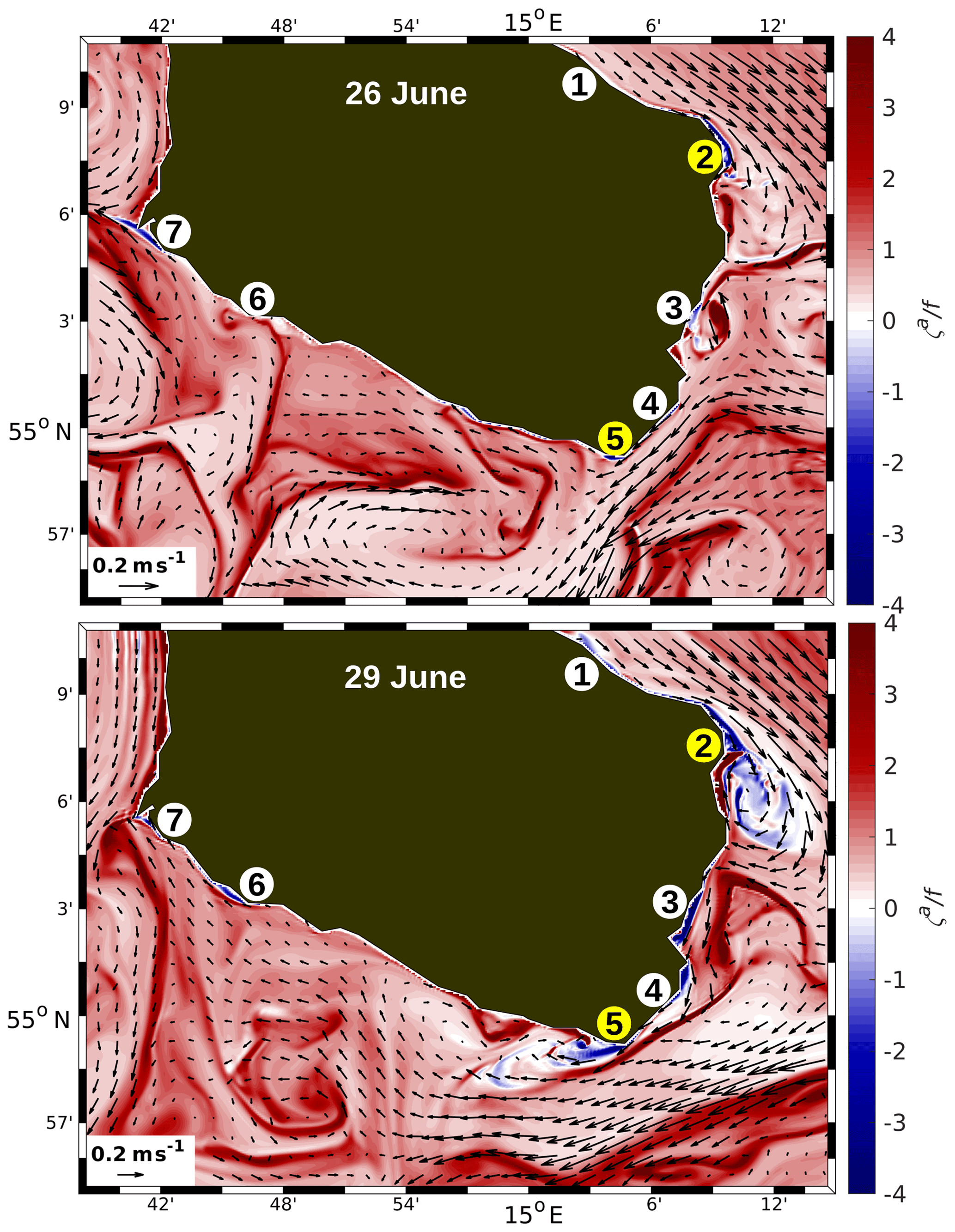
Figure 13R100: normalized absolute vorticity, ζa∕f, in the surface layer of the waters around Bornholm on 26 and 29 June. Encircled numbers indicate near-coastal locations of . Yellow circles mark locations where inertial instabilities tend to grow offshore.
According to Thomas et al. (2013), symmetric instability occurs when
with
and
Here,
is the Richardson number of the geostrophic flow,
is the buoyancy,
is the squared Brunt–Väisälä frequency, and
is the absolute vorticity of the geostrophic flow . ρ0 is a constant reference density, and is g the gravitational acceleration. Specifically, in regions where (cyclonic vorticity), symmetric instability prevails if the conditions
are satisfied. By contrast, symmetric instability is the dominant mode of instability in regions of anticyclonic vorticity () if
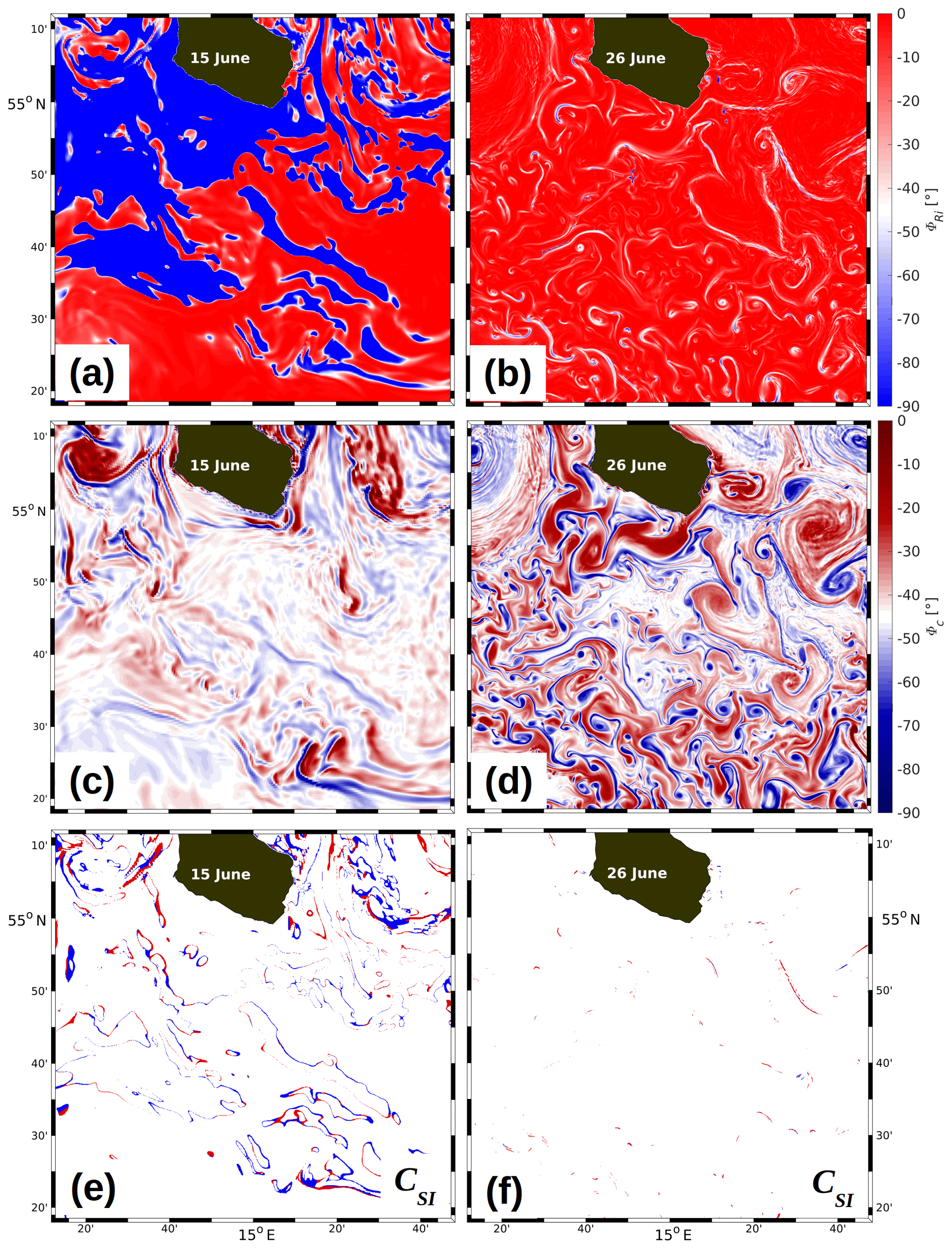
Figure 14R100: (a, b) ϕRi, (c, d) ϕc, and (e, f) CSI at 2 m of depth on 15 (left) and 26 June (right). Panels (e) and (f) are logical maps indicating where the condition for symmetric instability, CSI, is satisfied in regions of cyclonic (red) and anticyclonic (blue) absolute vorticity according to Eqs. (17) and (18), respectively. For an explanation of the other symbols, see the text.
As the condition described by Eq. (10) must be satisfied in the mixed layer for symmetric instability to occur, all above quantities were evaluated in R100 at 2 m of depth. Note that the relative vorticity is identical to the relative vorticity of the geostrophic flow because ζ is the curl of the rotational, divergence-free part of the total velocity, which is the geostrophic velocity by definition. Hence, a decomposition of the total velocity in a geostrophic part Vgeo and an ageostrophic part Vageo requiring a Poisson solver is redundant (for some test cases, both ζgeo and ζ were evaluated, showing identical results). For simplification, the subscript “geo” will therefore be dropped for and Rigeo. Figure 14 shows ϕRi, ϕc, and CSI at the start of the model integration on 15 June (using as an initial condition the corresponding field mapped from R500 on the 100 m grid) and on 26 June. On 15 June, there are large areas where (Fig. 14a, in blue), indicating satisfaction of the first condition of Eqs. (17) and (18). However, this condition is only necessary and sufficient for regions of cyclonic vorticity (). Considering the second condition in Eq. (18), necessary and sufficient conditions for regions of anticyclonic vorticity are satisfied if, and only if, . Linking the requirements for ϕc (Fig. 14c) and ϕRi yields the logical map in Fig. 14e for 15 June, indicating where Eqs. (17) and (18) are satisfied for cyclonic and anticyclonic vorticity, respectively. Compared to the fairly widespread areas where the necessary conditions for ϕRi and ϕc are met separately, the necessary and sufficient conditions for CSI are satisfied only in rather limited streaks. On 26 June, 9 d later, there are just a few spots where even CSI is satisfied (Fig. 14f). Hence, favourable conditions for symmetric instability prevail only during the initial phase of the model integration, becoming less frequent thereafter. More insight into the temporal evolution of the statistics of CSI is provided by the relative frequency of occurrence, , where n is the number of grid cells in which the criterion for CSI is met, and N is the total number of grid cells. p(CSI) decays from 4.8 % on 15 June to 1.8 % on 16 June, which yields an e-folding scale of ≈1 d comparable to the inertial period of 14.6 h at this latitude. Thereafter, p(CSI) decreases almost steadily and stabilizes around 0.5 %. Hence, as symmetric instability extracts kinetic energy from the geostrophic flow at a rate given by the geostrophic shear production (Thomas et al., 2013), this process comes rapidly due to a halt after about one inertial period and mixed-layer instability presumably takes over. p(CSI) was also computed for the R100 model run with atmospheric forcing (see above Sect. 4.3). In that run, p(CSI) increased strongly on 18, 21, 24, and 27 June, which were the times of the wind bursts (see Fig. 3), and slackened thereafter. Thus, the conditions favouring symmetric instability are re-established during strong wind events by the build-up of kinetic energy, and as soon as the wind slackens, the energy is released.
Mixed-layer instability is an efficient mechanism to restratify the mixed layer (Boccaletti et al., 2007). For the determination of the mixed-layer depth, MLD, a Δσθ=0.1 kg m−3 criterion was used; i.e. MLD was defined as the depth at which the potential density exceeds the surface density for the first time by Δσθ. The domain-wide mean MLD decreases almost linearly from 12.7 m on 15 June to 5.1 m on 29 June. Hence, the mixed layer is restratified, probably by mixed-layer instability. In order to exclude the possibility that symmetric instability drives the restratification, the relative frequency of occurrence, , was computed. This quantity drops from 23.2 % to 4.0 % within the first day of the integration and slowly decreases thereafter to 1.4 % on 29 June. Hence, after about one inertial period, Ri≥1 almost everywhere, which makes symmetric instability unlikely. This is in accordance with Haine and Marshall (1998), who state that “symmetric instability rapidly generates a layer with vanishing potential vorticity (Ri=1), but non-zero vertical stratification. Thereafter a nonhydrostatic baroclinic instability develops …”.
4.4.4 Frontal circulation
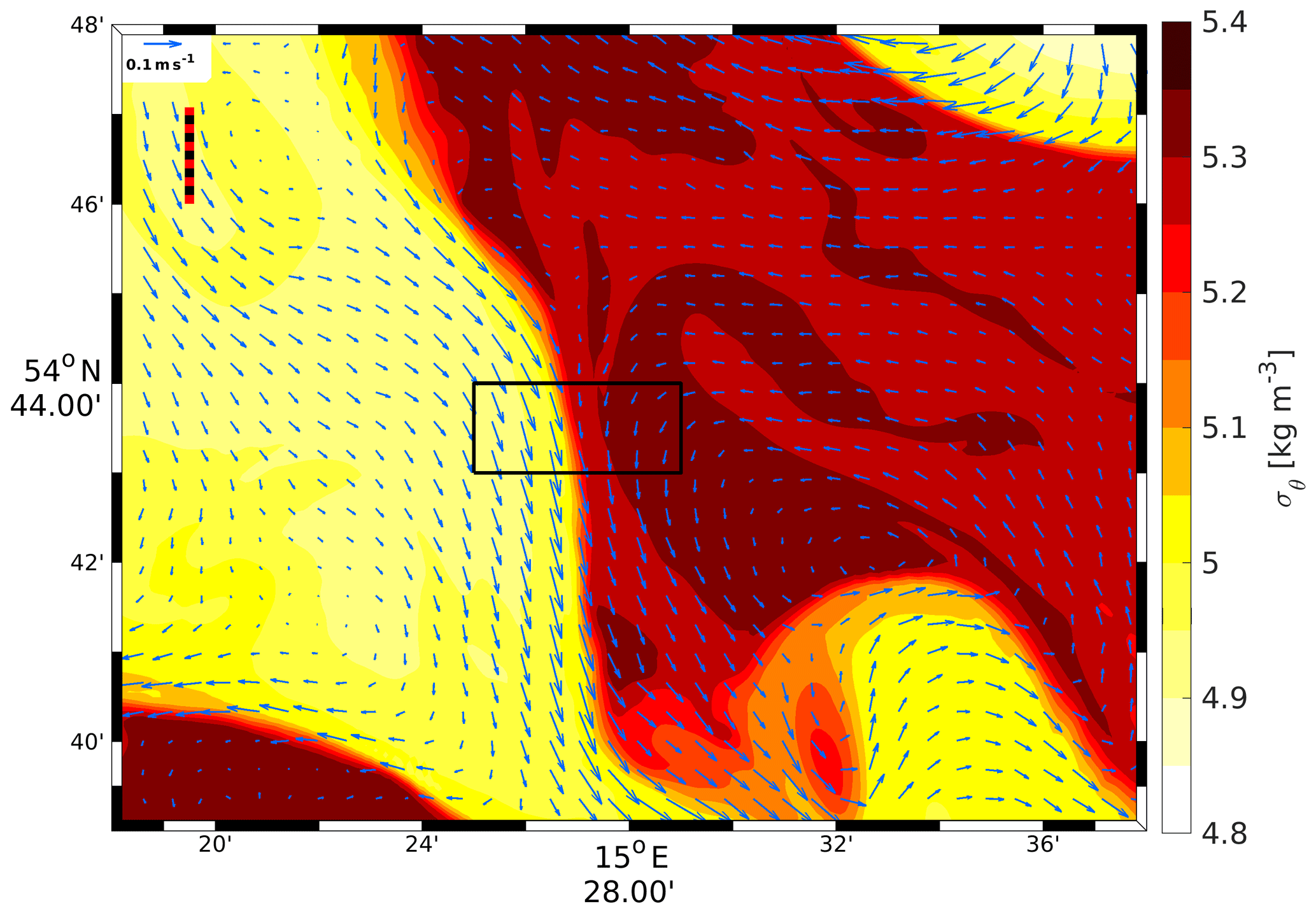
In order to provide details on the secondary circulation in submesoscale fronts in a non-idealized model, features resembling the confluence situation as provided by a deformation field were identified in the R100 fields of 26 June in the red box indicated in Fig. 7d. Here, dense water in the east and light water in the west form a confluent flow pattern and generate a density contrast at the surface of more than 0.4 kg m−3 over a horizontal distance of about 2 km within the black rectangle shown in Fig. 15.
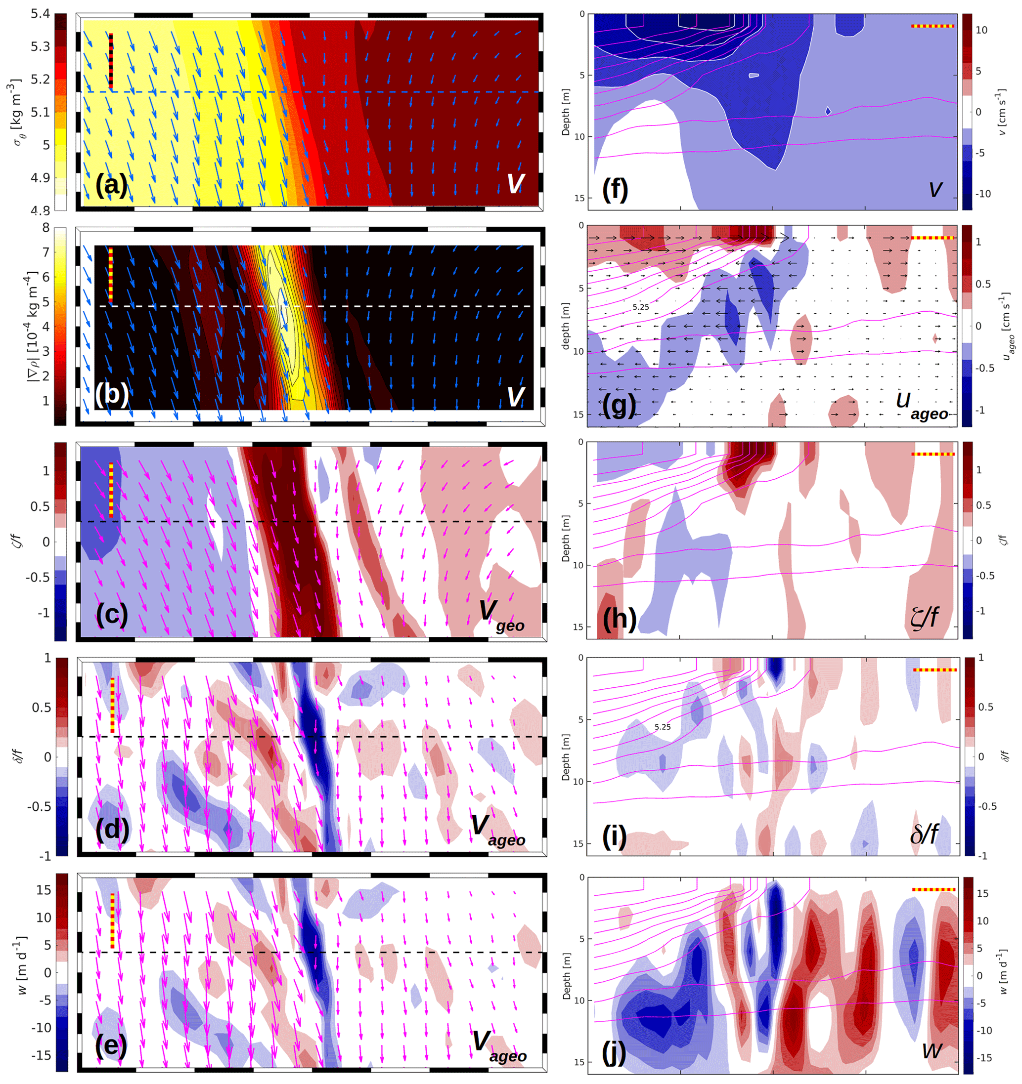
Figure 16 R100, 26 June: maps of dynamical quantities within the black box in Fig. 15; (a) σθ and V, (b) and V, (c) ζ∕f and Vgeo, and (d) δ∕f and Vageo in the top layer, as well as (e) w and Vageo at the bottom of the top layer. Velocity vectors are drawn at a resolution of 200 m. Vertical sections of (f) v, (g) uageo, (h) ζ∕f, (i) δ∕f, and (j) w. Contour lines of potential density anomaly σθ are magenta and spaced at the same intervals as in (a). The horizontal dashed lines in the centres of (a)–(e) indicate the position of the zonal sections displayed in (f)–(j). In either subplot, the dashed rulers represent a horizontal distance of 500 m.
Detailed maps of various quantities within that rectangle are displayed in Fig. 16a–e, and vertical cross sections along the dashed lines are shown in Fig. 16f–j. In the western part of the front, the total velocity vectors at the surface are aligned almost parallel to the isopycnals (panel a); extreme values of are close to 12 cm s−1 at the surface. In the cross section (panel f), the v component attains minimum values of cm s−1, located a few hundred metres to the west of the maximum horizontal density gradient (panel b). The velocity field depicts the classical picture of a frontal jet, with a width of about 3 km and a depth of around 4 m. It is defined by the −6 cm s−1 isotach of the v component. The horizontal shear of the jet creates a front-parallel band of strong cyclonic relative vorticity with maximum values of >1.6f (panels c, h). The cross-front width of the band is about 600 m, and the highest values of the relative vorticity are congruent with the maximum horizontal density gradient (panel b). A wide band of anticyclonic relative vorticity extends to the west of the cyclonic region. East of the cyclonic region, several bands with alternating sign are aligned. Vectors of Vgeo are superimposed in panel (c). A comparison with panels (a) and (c) reveals that the directions of V and Vgeo closely resemble each other in appearance, but the speeds are slightly different. While the maximum speeds of V are around 12 cm s−1 in the jet, those of Vgeo are close to 10 cm s−1; i.e. the jet is super-geostrophic (Persson, 2001). This is confirmed by panel (d), which shows the horizontal divergence δ∕f, together with the vectors of the ageostrophic flow Vageo. The meridional components of Vageo and Vgeo have the same (negative) sign, and hence Vageo amplifies the geostrophic jet. The maximum ageostrophic speeds are around 6 cm s−1. In the cross-frontal direction (panel g), the 5.25 kg m−3 isopycnal separates two regimes of opposite zonal component of the ageostrophic flow, uageo. In the lighter water, uageo>0, and uageo<0 in the heavier water. While the overall magnitude of uageo is just a few millimetres per second, it attains its highest value of about 1 cm s−1 right at the location of the surface outcrop of the 5.25 kg m−3 isopycnal.
The impact of Vageo on the divergence δ and on the vertical speed w is illustrated in Fig. 16d, i, e, and j. According to panels (d) and (i), extreme values of and are found at the sea surface immediately to the west and to the east of the maximum horizontal density gradient, respectively. The minimum of the divergence (maximal convergence) drives a deep-reaching downwelling cell with extreme speeds of almost 15 m d−1. Less intense upwelling of a maximum of ≈6 m d−1 is associated with the divergence maximum (panel j). The positions of the extrema of δ∕f are also reflected by its horizontal surface distribution in panel (d), while a comparison of panels (d) and (e) reveals a clear correlation between δ and w. Patches of convergent motion are also found along the 5.25 kg m−3 isopycnal in panel (i); potentially, they feed the large downwelling area underneath it. Further cells of intense vertical motion are found west and east of the surface front as shown in panel (j). Apparently, these patterns are not parts of the secondary circulation but are rather caused by internal waves (see Sect. 4.2.3) or by another weak front located about 600 m further east.
Overall, the described secondary circulation pattern closely resembles the ones of the idealized model studies mentioned in the Introduction; primarily, this is a “single overturning cell with upwelling and surface divergence on the light side and downwelling and surface convergence on the dense side” (literally after McWilliams, 2016). However, Fig. 16 provides additional details which were potentially not yet highlighted before.
-
The frontal jet is super-geostrophic; i.e. the jet speed is amplified by an ageostrophic component. Under the assumption that the jet was in geostrophic balance, the theoretical inclination of the front was calculated as 0.003∘ using the Margules equation (Margules, 1906). Assuming the σθ=5.25 kg m−3 isopycnal as the frontal interface, the tilt angle of that isopycnal was, however, only 0.001∘. Hence, the slope of the front is not in geostrophic balance with the jet. This circumstance was not considered in the previous literature assuming two dimensionality (Bleck et al., 1988) or quasi-geostrophic (Nagai et al., 2006) or semi-geostrophic (Thompson, 2000) balance. In contrast, in the model of McWilliams (2017) (see Fig. 5 there), the ageostrophic contribution to the jet speed amounts to about 3 cm s−1, while the geostrophic fraction is close to 12 cm s−1.
-
The maximum speed of the cross-frontal ageostrophic velocity is weaker than expected from earlier models. Right at the surface, it is only 1 cm s−1, while Bleck et al. (1988) arrived at >4.5 cm s−1 and McWilliams (2017) at least at 2 cm s−1. A potential reason for this discrepancy is that the other studies did not consider the ageostrophic velocity to be the ageostrophic part of the total flow but rather the departure from the (barotropic) deformation velocity or from the far-field average instead. In the present situation, it was not possible to separate the total flow into such components because they were not defined. Hence, one may speculate that something like the deformation velocity is opposed to the cross-front ageostrophic velocity and attenuates it.
-
According to Fig. 16g, the cross-frontal velocity is positive (eastward) in the light water (σθ<5.25 kg m−3) and westward in the denser water below. Thus, the velocity converges at that isopycnal, in accordance with Fig. 16i. It is not known to the authors whether such a “sloping convergence” was mentioned before in the oceanographic literature.
The investigated front satisfies the criteria to be denoted as “submesoscale”. The first criterion, Ro∼𝒪(1), is confirmed by Fig. 16c and h, indicating that the f-scaled relative vorticity (which is equivalent to a local Rossby number) is 𝒪(1). Another criterion is Ri∼𝒪(1) (Thomas et al., 2008; Mahadevan, 2016). According to Fig. 17, Ri≈2 in the frontal region at the location of maximum convergence at the sea surface.
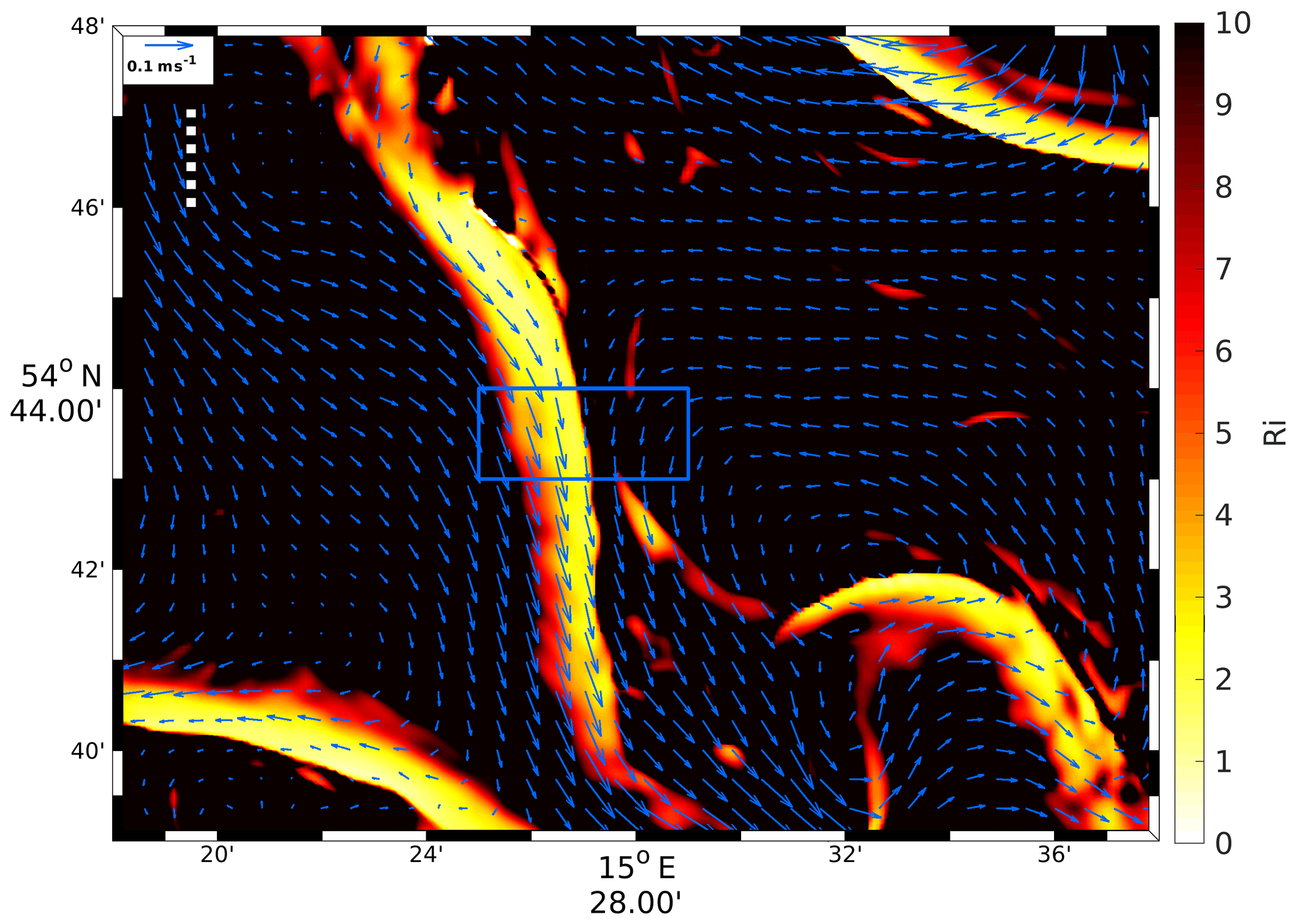
Figure 17R100, 26 June: Richardson number Ri at 2 m of depth and total top-layer velocity V drawn at 600 m resolution. For the position of the area, see the red box in Fig. 7d. The magenta box indicates the position of the maps shown in Fig. 16a–e. It is identical to the black box in Fig. 15. The dashed ruler represents a distance of 2 km.
The R100 results presented above have provided a detailed insight into STPPs, such as tracer patterns, kinematic structures, and dynamical processes related to fronts and eddies. A comparison with observations, however, is rather limited because STPPs are difficult to measure due to their small spatial and temporal scales. Moreover, the R100 results are obtained from a run without atmospheric forcing, and it would be legitimate to compare them only with situations in which the air–sea fluxes of momentum, heat, and fresh water are minimum. However, the atmospheric conditions, not to mention the air–sea fluxes, when the observations were taken are mostly not described. Hence, the comparisons below based on a few statistical numbers and qualitative similarities should be handled with care.
Kinematic quantities of STPPs were obtained from direct measurements in the framework of LatMix and SubEx. Shcherbina et al. (2013) presented a detailed view of submesoscale vorticity, divergence, and strain statistics from synchronous two-ship ADCP (acoustic Doppler current profiler) samplings. Specifically, their observations indicated flows with Ro∼𝒪(1) and an asymmetry in the distribution of the relative vorticity skewed towards positive values. The latter is in excellent agreement with the R100 results. By contrast, Ohlmann et al. (2017) identified STTPs with aerial guidance and seeded them with drifters. The Lagrangian observations exhibited high values of relative vorticity and divergence exceeding 5f, suggesting vertical velocities up to 240 m d−1. Such values are rather close to the peak values obtained from R100. Similar values for ζ∕f and δ∕f also resulted from the high-frequency radar observations of Parks et al. (2009). As the observations mentioned above are two-dimensional and confined to the sea surface, they provide only limited information on the subsurface properties of STPPs. Somewhat more detailed insight is gained from the high-resolution in situ measurements of Zhong et al. (2017), which exhibit submesoscale kinematic structures along a vertical section through a 200 km wide mesoscale eddy in the South China Sea. Unfortunately, that eddy is an anticyclone, and a comparison with the corresponding quantities in C3 is problematic.
The formation of a the submesoscale cyclonic eddy C3 (Fig. 12) closely resembles the sequence of infrared images published by Munk et al. (2000) (see Fig. 12 there) and the snapshot of Buckingham et al. (2017). In both cases, the eddies originate from an unstable thermal front which finally breaks up in a train of cyclonic eddies. While the diameters of the eddies shown by Munk et al. (2000) are around 10 km (very rough visual estimate), those of Buckingham et al. (2017) are smaller (1–10 km according to the authors).
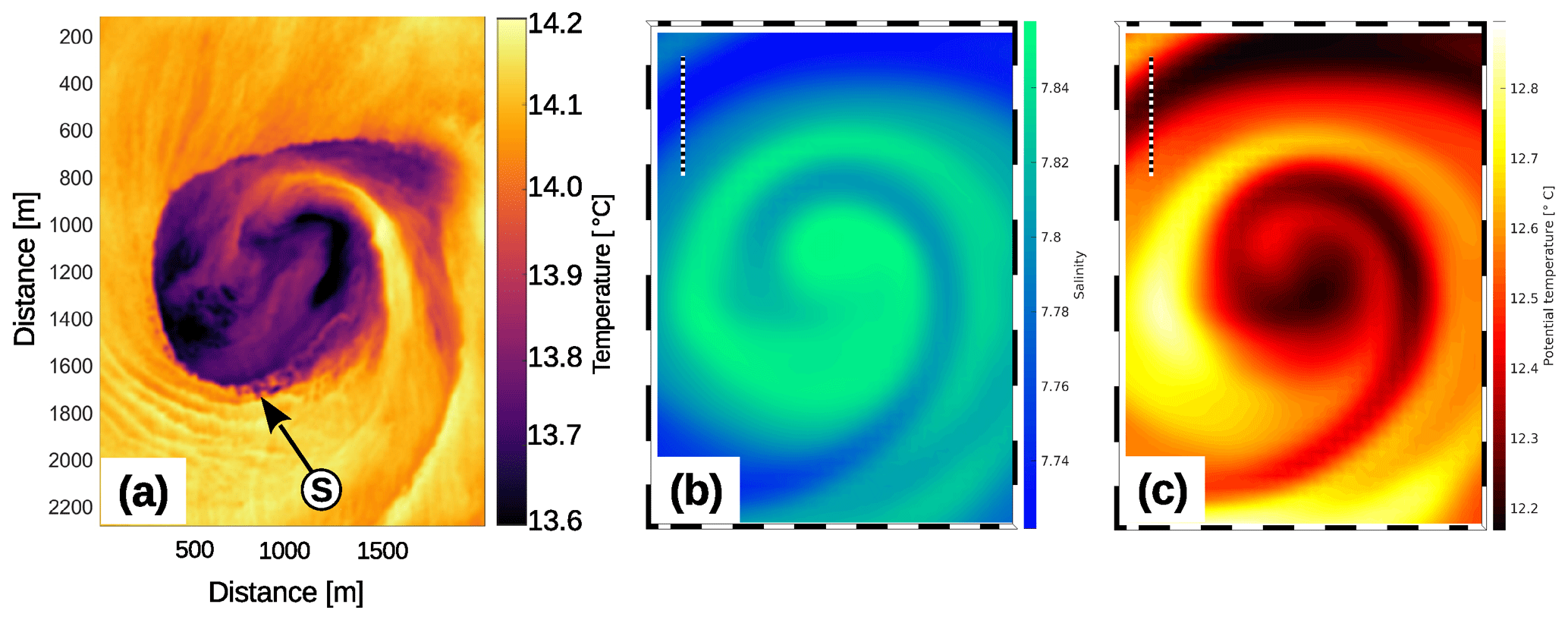
Figure 18Tracer patterns of submesoscale eddies. (a) Observed sea surface temperature of a cyclonic eddy in the Southern California Countercurrent. The image was taken on 1 February 2013 at 20:34 in the framework of SubEx (Marmorino et al., 2018). (b) Modelled salinity and (c) potential temperature of the cyclone C3 on 26 June at 15 m of depth (see Figs. 11 and 12). Cold water spots in (a) are denoted by “S”. The dashed rulers in (b) and (c) represent a distance of 1 km.
A close-up infrared image of an eddy observed in the Southern California Bight is shown in Fig. 18, together with corresponding properties from the modelled cyclone C3 (see Figs. 11, 12). The observed sea surface temperature (panel a) exhibits a spiraliform cyclonic eddy with a diameter of about 1 km; the diameter is estimated as the width between the ≈13.8 ∘C isotherms (purple) on either side. Special features are the low-temperature patches (black) close to the eddy centre, suggesting upwelling, and the bright ripples in the southwest which are probably caused by internal waves. One may also note the cold spots “S” along the periphery; they are definitely not caused by a malfunction of the camera because they show up at different positions in a sequence of images taken within a period of about 20 min. Potentially, they are created by intense vertical mixing (see Marmorino et al., 2013 and Fig. 2 in Marmorino et al., 2018). For comparison with C3, the potential temperature and salinity at 15 m of depth are provided in panels (b) and (c). This depth was selected as the mixed-layer depth at the corresponding position in R100 is about 9 m and the surface signal of C3 is hardly resolved (see potential temperature and salinity on 26 June in Fig. 5). The overall structures of the C3 salinity and the sea surface temperature of the observed eddy look similar, but the smaller details visible in the latter are not reproduced by C3: these are the ripples in the southwest, the cold spots, and the texture of the tracer field in the core. Most probably, this is due to the insufficient horizontal resolution of R100 or nonhydrostatic effects which are not included in the applied ROMS version.
There are two observational studies available regarding necessary instability criteria at fronts (Thomas et al., 2013; Zhong et al., 2017), but they are not comparable to the maps in Fig. 14 because the criteria were computed along vertical sections across the Gulf Stream front and in a large anticyclonic eddy in the South China Sea, respectively. Concerning frontogenetic or frontolytic processes, computations or estimations of the components of the frontal tendency equation from observational data are not known to the authors.
Comprehensive observations of the frontal circulation (Pollard and Regier, 1992; Rudnick, 1996; Pallàs-Sanz et al., 2010) confirm the secondary circulation pattern as predicted from theoretical considerations and numerical models. However, the above studies did not resolve STTPs, and the extrema of the vertical velocity are correspondingly low with 𝒪(10 m d−1). Namely, the vertical velocities in the front shown in Fig. 16e and j are of the same order, but this is due to the low water depth. On the contrary, the higher-resolution observations of a submesoscale front oriented along the periphery of a mesoscale eddy (Adams et al., 2017) confirm vertical velocities of 𝒪(100 m d−1). Moreover, it was demonstrated that within the same front there were confluent and diffluent regions of the cross-frontal velocity. This does not necessarily prove that the ageostrophic velocity changes sign, but it indicates that the generally accepted picture of the secondary circulation is only valid in the case of frontogenesis driven by an externally imposed deformation field.
A double one-way nesting approach is used in order to simulate submesoscale turbulent patterns and processes (STPPs) in the southern Baltic Sea in summer 2016. In order to reproduce the mesoscale environment in a realistic way, the Regional Ocean Modeling System (ROMS) with 500 m horizontal resolution (R500) is nested in an existing operational model, and further downscaling to a grid size of 100 m (R100) enables the generation of STPPs.
In R500, the kinematic and dynamical structures are rather sensitive to the surface boundary conditions. While the response of mesoscale patterns to turning off the atmospheric forcing is rather sluggish, it has an immediate impact on the generation of smaller-scale features which represent the low-wavenumber part of submesoscale turbulence in the spectral range around 5 km.
In R100, the atmospheric forcing is turned off from the outset because the air–sea fluxes inhibit the growth of STTPs. Thus, the R100 results represent situations that occur only under quasi-adiabatic conditions. In nature, such situations are approximated in no-wind or light-wind conditions which offer the best chance to observe STPPs. On the other hand, the R100 findings must not be compared to observations which are taken during stronger wind. Moreover, as the R100 findings reflect summer conditions in the Baltic Sea, they must not be applied to another season or any other region of the World Ocean.
The horizontal density gradients in R100 grow for about 10 d, and afterwards the frequency of occurrence of strong gradients begins to decline, indicating frontal arrest as soon as the absolute horizontal density gradient reaches a critical value. STPPs develop rapidly within about a day; they are characterized by relative vorticities and divergences reaching multiples of the Coriolis parameter, whereby the frequency distribution of relative vorticity is clearly biased towards negative (anticyclonic) values. Vertical velocities of 𝒪(100) m d−1 are diagnosed in R100. However, as the vertical motion is predominantly controlled by internal waves and to a lesser extent by frontal secondary circulations, estimates of the vertical velocities associated with submesoscale processes are 1 order of magnitude less.
Typical elements of the secondary circulation of two-dimensional strain-induced frontogenesis are identified at an exemplary front in shallow water; these are the frontal jet, downwelling on the dense side, and upwelling on the less dense side. In addition to the results of idealized two-dimensional models, details of the ageostrophic current field and the related divergence are revealed: the frontal jet is not in geostrophic balance but is super-geostrophic instead. Further on, it is shown that a region of enhanced convergent flow is aligned with the slope of the frontal surface.
The components of the tendency equation are evaluated in a subregion of the R100 domain. At fronts, frontogenetic and frontolytic processes represented by the frontogenetic tendency, F, and the contributions from the straining deformation of the geostrophic and vertical velocity, Qgeo and Qw, respectively, are equi-partitioned, bimodal, and of the same order of magnitude. By contrast, the contributions from the ageostrophic velocity, Qageo, and from vertical mixing, Qdv, act primarily frontogenetic, while the contribution from horizontal mixing, Qdh, is negligible everywhere.
The conditions for two types of hydrodynamic instability are evaluated for the whole R100 domain: favourable conditions for inertial (centrifugal) instability are found only along coastlines. There, anticyclonic eddies develop rapidly from along-coast currents if the coast is on the right-hand side (looking downstream) and if the coastline is anticyclonically curved. During the first day of the R100 integration, symmetric instability is likely to occur in about 5 % of the model domain, but within 2 d, the probability drops to <1 %. Parallel to the rapidly decreasing probability are increases in the geostrophic Richardson number Rigeo. While at the beginning of the integration, Rigeo<1 in about 24 % of the R100 domain, this number decreases to about 4 % after 1 d, indicating that mixed-layer instability is the main process depleting the reservoir of potential energy.
While anticyclonic eddies are generated solely along coastlines due to inertial instability, cyclonic eddies are found in the entire R100 domain but preferably in those regions where the water depth is less than about 40 m. A special feature of the cyclones is their ability to absorb internal waves and to sustain patches of continuous upwelling for several days, favouring plankton growth (Mahadevan, 2016). In contrast to mesoscale cyclones which pinch off from basin-scale fronts, submesoscale cyclones are rolled-up streamers, similar to those observed by Klymak et al. (2016) on the north wall of the Gulf Stream. Hence, it may not be appropriate to denote these features as “eddies” but “spirals” instead, as suggested by Munk et al. (2000).
Peculiar features of the observed eddy shown in Fig. 18a are the cold spots along its periphery. It is conjectured that the spots are small upwelling cells probably driven by gravitational instability, which links the submesoscale with the microscale and finally leads to three-dimensional energy dissipation. As it is extremely challenging to observe such features with in situ methods, attempts will be made to catch these spots with further downscaling to the 𝒪(1) m scale using nonhydrostatic models or large eddy simulations. These numerical approaches would also serve to explore structures and processes in the interior of eddies in greater detail.
The model code and the output of the ROMS runs presented in this article are available from the first author on request. A video of the evolution of the submesoscale spiral shown in Fig. 12 is available at https://doi.org/10.5446/46222 (Onken et al., 2020).
RO implemented the double-nested ROMS model for the given region in the Baltic Sea and conducted the model runs. IMA-B and BB contributed the results from SubEx in the Southern California Countercurrent, and BB coordinated Expedition Clockwork Ocean and the corresponding modelling activities.
The authors declare that they have no conflict of interest.
We thank Rüdiger Röttgers and Hajo Krasemann for the processing of Fig. 4b and Rainer Feistel, who provided details of the Arkona and Bornholm basins to us. Geoffrey Smith and George Marmorino, Naval Research Laboratory, provided infrared observations taken during the Submesoscale Experiment for comparison. The ICON-EU output was made available by Thomas Bruns of the German Weather Service (DWD). The output of the HIROMB-BOOS model was downloaded from the Copernicus Marine Environment Monitoring Service, and the bathymetry data from the General Bathymetric Chart of the Oceans were provided by the British Oceanographic Data Centre. The coastline data were obtained from NOAA (National Oceanic and Atmospheric Administration).
The article processing charges for this open-access publication were covered by a Research Centre of the Helmholtz Association.
This paper was edited by Markus Meier and reviewed by four anonymous referees.
Adams, K. A., Hosegood, P., Taylor, J. R., Sallée, J. B., Bachman, S., Torres, R., and Stamper, M.: Frontal circulation and submesoscale variability during the formation of a Southern Ocean mesoscale eddy, J. Phys. Oceanogr., 47, 1737–1753, https://doi.org/10.1175/JPO-D-16-0266.1,2017. a
Berg, P.: Mixing in HBM. DMI Scientific Report, 12-03, Danmarks Meteorologiske Institut, København, Denmark, 2012. a
Bleck, R., Onken, R., and Woods, J. D.: A two-dimensional model of mesoscale frontogenesis in the ocean, Q. J. Roy. Meteor. Soc., 114, 347–371, 1988. a, b, c, d
Blumen, N.: On short-wave baroclinic instability, J. Atmos. Sci., 36, 1925–1933, 1979. a
Boccaletti, G., Ferrari, R., and Fox-Kemper, B.: Mixed layer instabilities and restratification, J. Phys. Oceanogr., 37, 2228–2250, https://doi.org/10.1175/JPO3101.1, 2007. a, b, c
Buckingham, C. E., Khaleel, Z., Lazar, A., Martin, A. P., Allen, J. T., Naveira Garabato, A. C., Thompson, A. F., and Vic, C.: Testing Munk's hypothesis fur submesoscale eddy generation using observations in the North Atlantic, J. Geophys. Res.-Oceans, 122, 6725–6745, https://doi.org/10.1002/2017JC012910, 2017. a, b
Capet, X., McWilliams, J. C., Molemaker, M. J., and Shchepetkin, A. F.: Mesoscale to submesoscale transition in the California Current system. Part I: flow structure, eddy flux, and observational tests, J. Phys. Oceanogr., 38, 29–43, https://doi.org/10.1175/2007JPO3671.1, 2008a. a
Capet, X., McWilliams, J. C., Molemaker, M. J., and Shchepetkin, A. F.: Mesoscale to submesoscale transition in the California Current system. Part II: frontal processes, J. Phys. Oceanogr., 38, 44–64, https://doi.org/10.1175/2007JPO3672.1, 2008b. a, b, c, d
Capet, X., McWilliams, J. C., Molemaker, M. J., and Shchepetkin, A. F.: Mesoscale to submesoscale transition in the California Current system. Part III: energy balance and flux, J. Phys. Oceanogr., 38, 2256–2269, https://doi.org/10.1175/2008JPO3810.1, 2008c. a
Chapman, D. C.: Numerical treatment of cross-shelf open boundaries in a barotropic coastal ocean model, J. Phys. Oceanogr., 15, 1060–1075, 1985. a
Charney, J. G.: Geostrophic turbulence, J. Atmos. Sci., 28, 1087–1095, 1971. a
Charney, J. P.: The dynamics of long waves in a baroclinic westerly current, J. Meteorol., 4, 135–163, 1947. a
Dewar, W. K., McWilliams, J. C., and Molemaker, M. J.: Centrifugal instability and mixing in the California Undercurrent, J. Phys. Oceanogr., 45, 1224–1241, https://doi.org/10.1175/JPO-D-13-0269.1, 2015. a, b
Eady, T.: Long waves and cyclone waves, Tellus, 1, 33–52, 1949. a
Eliassen, A.: On the vertical circulation in frontal zones, Geofysiske Publikasjoner, 24, 147–160, 1962. a
Fairall, C. W., Bradley, E. F., Rogers, D. B., Edson, J. B., and Young, G. S.: Bulk parameterization of air-sea fluxes for Tropical Ocean-Global Atmosphere Coupled-Ocean Atmosphere Response Experiment, J. Geophys. Res., 101, 3747–3764, https://doi.org/10.1029/95JC03205, 1996. a
Feistel, R., Nausch, G., and Wasmund, N. (Eds.): State and Evolution of the Baltic Sea, 1952–2005: A Detailed 50-year Survey of Meteorology and Climate, Physics, Chemistry, Biology, and Marine Environment, Wiley-Interscience, Hoboken, New Jersey, USA, ISBN 978-0-471-97968-5, 2008. a
Fennel, W., Seifert, T., and Kayser, B.: Rossby radii and phase speeds in the Baltic Sea, Cont. Shelf Res., 11, 23–26, 1991. a
Fox-Kemper, B. and Ferrari, F.: Parameterization of mixed layer eddies. Part I: theory and diagnosis, J. Phys. Oceanogr., 38, 1145–1165, https://doi.org/10.1175/2007JPO3792.1, 2008. a
Früh, W.-G.: Amplitude vacillation in baroclinic flows, in: Modelling Atmospheric and Oceanic Flow: Insights from laboratory experiments and numerical simulations, edited by: von Larcher, T. and Williams, P. D., Wiley, 61–81, https://doi.org/10.1002/9781118856024, 2015. a
Gula, J., Molemaker, M. J., and McWilliams, J. C.: Submesoscale cold filaments in the Gulf Stream, J. Phys. Oceanogr., 44, 2617–2643, https://doi.org/10.1175/JPO-D-14-0029.1, 2014. a, b, c, d
Gula, J., Molemaker, M. J., and McWilliams, J. C.: Submesoscale dynamics of a Gulf Stream frontal eddy in the South Atlantic Bight, J. Phys. Oceanogr., 46, 305–325, https://doi.org/10.1175/JPO-D-14-0258.1, 2016a. a
Gula, J., Molemaker, M. J., and McWilliams, J. C.: Topographic generation of submesoscale centrifugal instability and energy dissipation, Nat. Commun., 7, 12811, https://doi.org/10.1038/ncomms12811, 2016b. a, b
Gurova, E. and Chubarenko, B.: Remote-sensing observations of coastal sub-mesoscale eddies in the south-eastern Baltic, Oceanologia, 54, 631–654, https://doi.org/10.5697/oc.54-4.631, 2012. a
Haine, T. W. N. and Marshall, J.: Gravitational, symmetric, and baroclinic instability of the ocean mixed layer, J. Phys. Oceanogr., 28, 634–658, 1998. a, b, c
Haney, R. L.: On the pressure gradient force over steep topography in sigma coordinate models, J. Phys. Oceanogr., 21, 610–619, 1991. a
Haidvogel, D. B., Arango, H. G., Hedstrøm, K., Beckmann, A., Malanotte-Rizzoli, P., and Shchepetkin, A. F.: Model evaluation experiments in the North Atlantic Basin: simulations in nonlinear terrain-following coordinates, Dynam. Atmos. Oceans, 32, 239–281, 2000. a, b
Hide, R.: An experimental study of thermal convection in a rotating liquid, Philos. T. R. Soc. Lond. A, 250, 441–478, 1958. a
Holton, J.: The role of gravity induced drag and diffusion in the momentum budget of the mesosphere, J. Atmos. Sci., 39, 791–79, 1982. a, b
Holton, J. R.: An introduction to dynamic meteorology, Fourth edition, Elsevier Academic Press, ISBN 0-12-354016-X, 2004.
Hoskins, B. J.: The mathematical theory of frontogenesis, Annu. Rev. Fluid Mech., 14, 131–151, 1982. a
Kantha, L. H. and Clayson, C. A.: An improved mixed-layer model for geophysical applications, J. Geophys. Res., 99, 25235–25266, 1994. a
Karimova, S. and Gade, M.: Improved statistics of submesoscale eddies in the Baltic Sea retrieved from SAR imagery, Int. J. Remote Sens., 37, 2394–2414, https://doi.org/10.1080/01431161.2016.1145367, 2016. a
Klymak, J. M., Shearman, R. K., Gula, J., Lee, C. M., D'Asaro, E. A., Thomas, L. N., Harcourt, R. R., Shcherbina, A. Y., Sundermeyer, M. A., Molemaker, J., and McWilliams, J. C.: Submesoscale streamers exchange water on the north wall of the Gulf Stream, Geophys. Res. Lett., 43, 1226–1233, https://doi.org/10.1002/2015GL067152, 2016. a
Kubryakov A. A. and Stanichny, S. V.: Seasonal and interannual variability of the Black Sea eddies and its dependence on characteristics of the large-scale circulation, Deep-Sea Res. Pt. I, 97, 80–91, https://doi.org/10.1016/j.dsr.2014.12.002, 2015. a
Large, W. G., McWilliams, J. C., and Doney, S. C.: Oceanic vertical mixing: a review and a model with a nonlocal boundary layer parameterization, Rev. Geophys., 32, 363–403, 1994. a
Lévy, M., Ferrari, R., Franks, P. J. S., Martin, A. P., and Rivière, P.: Bringing physics to life at the mesoscale, Geophys. Res. Lett., 39, L14602, https://doi.org/10.1029/2012GL052756, 2012. a
Leppäranta, M. and Myrberg, K. (Eds.): Physical Oceanography of the Baltic Sea, Springer, Berlin, ISBN 978-3-540-79702-9, 2009. a
Magaard, L. and Rheinheimer, G. (Eds.): Meereskunde der Ostsee, Springer-Verlag, Berlin, 269 pp., 1974. a
Mahadevan, A.: The impact of submesoscale physics on primary productivity of plankton, Annu. Rev. Mar. Sci., 8, 161–184, https://doi.org/10.1146/annurev-marine-010814-015912, 2016. a, b, c
Mahadevan, A., Tandon, A., and Ferrari, R.: Rapid changes in mixed layer stratification driven by submesoscale instabilities and winds, J. Geophys. Res., 115, C03017, https://doi.org/10.1029/2008JC005203, 2010. a
Marmorino, G. O., Smith, G. B., and Miller, W. D.: Surface imprints of water-column turbulence: a case study of tidal flow over an estuarine sill, Remote Sens., 5, 3239–3258, https://doi.org/10.3390/rs5073239, 2013. a
Marmorino, G. O., Smith, G. B., North, R. P., and Baschek, B.: Application of airborne infrared remote sensing to the study of ocean submesoscale eddies, Front. Mech. Eng., 4, 10, https://doi.org/10.3389/fmech.2018.00010, 2018. a, b
Marchesiello, P., McWilliams, J. C., and Shchepetkin, A. F.: Open boundary conditions for long-term integration of regional ocean models, Ocean Model., 3, 1–20, 2001. a
Margules, M.: Über Temperaturschichtung in stationär bewegter und in ruhender Luft, Meteorol. Z., Hann-Volume, 243–254, 1906 (translated and edited by: Volken, E., Giesche, A., and Brönnimann, S.: On temperature stratification in resting and non-accelerated moving air, Meteorol. Z., 25, 795–804, https://doi.org/10.1127/metz/2016/0833, 2016). a
McWilliams, J. C.: Fluid dynamics at the margin of rotational control, Environ. Fluid Mech., 8, 441–449, https://doi.org/10.1007/s10652-008-9081-8, 2008. a, b
McWilliams, J. C.: Submesoscale currents in the ocean, P. Roy. Soc. A, 472, 20160117, https://doi.org/10.1098/rspa.2016.0117, 2016. a, b, c, d
McWilliams, J. C.: Submesoscale surface fronts and filaments: secondary circulation, buoyancy flux, and frontogenesis, J. Fluid Mech., 823, 391–432, https://doi.org/10.1017/jfm.2017.294, 2017. a, b, c
McWilliams, J. C.: A survey of submesoscale currents, Geosci. Lett., 6, 3, https://doi.org/10.1186/s40562-019-0133-3, 2019. a
McWilliams, J. C., Molemaker, M. J., and Olafsdottir, E. I.: Linear fluctuation growth during frontogenesis, J. Phys. Oceanogr., 39, 3111–3129, https://doi.org/10.1175/2009JPO4186.1, 2009. a
Molemaker, M. J., McWilliams, J. C., and Dewar, W. K.: Submesoscale instability and generation of mesoscale anticyclones near a separation of the California Undercurrent, J. Phys. Oceanogr., 45, 613–629, https://doi.org/10.1175/JPO-D-13-0225.1, 2015. a
Müller, P., McWilliams, J. C., and Molemaker, J.: The 2D/3D turbulence conundrum, in: Marine Turbulence: theories, observations and models, edited by: Baumert, H. Z., Simpson, J., and Sündermann, J., Cambridge University Press, Cambridge, 397–505, 2008. a
Munk, W., Armi, L., Fischer, K., and Zachariasen, F: Spirals on the sea, P. Roy. Soc. A, 456, 1217–1280, 2000. a, b, c
Nagai, T., Tandon, A., and Rudnick, D. L.: Two-dimensional ageostrophic secondary circulation at ocean fronts due to vertical mixing and large-scale deformation, J. Geophys. Res., 111, C09038, https://doi.org/10.1029/2005JC002964, 2006. a, b
Ohlmann, J. C., Molemaker, M. J., Baschek, B., Holt, B., Marmorino, G., and Smith, G.: Drifter observations of submesoscale flow kinematics in the coastal ocean, Geophys. Res. Lett., 44, 330–337, https://doi.org/10.1002/2016GL071537, 2017. a, b
Onken, R.: Mesoscale upwelling and density finestructure in the seasonal thermocline – a dynmical model, J. Phys. Oceanogr., 22, 11, 1257–1273, 1992.
Onken, R.: Validation of an ocean shelf model for the prediction of mixed-layer properties in the Mediterranean Sea west of Sardinia, Ocean Sci., 13, 235–257, https://doi.org/10.5194/os-13-235-2017, 2017. a
Onken, R., Baschek, B., and Angel-Benavides, I.: The evolution of a submesoscale spiral, Copernicus Publications, https://doi.org/10.5446/46222, 2020. a, b
Osínski, R., Rak, D., Walczowski, W., and Piechure, W.: Baroclinic Rossby radius of deformation in the southern Baltic Sea, Oceanologia, 52, 417–429, 2010. a, b
Pallàs-Sanz, E., Johnston, T. M. S., and Rudnick, D. L.: Frontal dynamics in a California Current System shallow front: 1. Frontal processes and tracer structure, J. Geophys. Res., 115, C12067, https://doi.org/10.1029/2009JC006032, 2010. a
Parks, A. B., Shay, L. K., Johns, W. E., Martinez-Pedraja, J., and Gurgel, K.-W.: HF radar observations of small-scale surface current variability in the Straits of Florida, J. Geophys. Res., 114, C08002, https://doi.org/10.1029/2008JC005025, 2009. a
Persson, A.: The Coriolis force and the geostrophic wind (Coriolis Part 5), Weather, 56, 267–272, https://doi.org/10.1002/j.1477-8696.2001.tb06589.x, 2001. a
Plougonven, R. and Snyder, C.: Inertia-gravity waves spontaneously generated by jets and fronts. Part I: Different baroclinic life cycles, J. Atmos. Sci., 64, 2502–2520, https://doi.org/10.1175/JAS3953.1, 2007. a
Pollard, R. T. and Regier, L. A.: Vorticity and vertical circulation at an ocean front, J. Phys. Oceanogr., 22, 609–625, 1992. a
Renault, L., McWilliams, J. C., and Gula, J.: Dampening of submesoscale currents by air-sea stress coupling in the Californian upwelling system, Sci. Rep.-UK, 8, 13388, https://doi.org/10.1038/s41598-018-31602-3, 2018. a
Rhines, P. B.: Geostrophic turbulence, Annu. Rev. Fluid Mech., 11, 401–441, 1979. a
Rudnick, D. L.: Intensive surveys of the Azores front 2. Inferring the geostrophic and vertical velocity fields, J. Geophys. Res., 101, 16291–16303, 1996. a
Shakespeare, C. J.: Spontaneous generation of internal waves, Phys. Today, 72, 34, https://doi.org/10.1063/PT.3.4225, 2019. a
Shakespeare, C. J. and Taylor, J. R.: The spontaneous generation of inertia-gravity waves during frontogenesis forced by large strain: theory, J. Fluid Mech., 757, 817–853, https://doi.org/10.1017/jfm.2014.514, 2014. a
Shchepetkin, A. F. and Williams, J. C.: A family of finite-volume methods for computing pressure gradient force in an ocean model with a topography-following vertical coordinate, 24 pp., available at: http://www.atmos.ucla.edu/~alex/ROMS/pgf1A.ps (last access: 10 March 2017), 2001. a
Shchepetkin, A. F. and McWilliams, J. C.: The Regional Ocean Modeling System (ROMS): A split-explicit, free-surface, topography following coordinates ocean model, Ocean Model., 9, 347–404, https://doi.org/10.1016/j.ocemod.2004.08.002, 2005. a, b
Shcherbina, A., D'Asaro, E., Lee, C., Klymak, J., Molemaker, M., and McWilliams, J. C.: Statistics of vertical vorticity, divergence, and strain in a developed submesoscale turbulence field, Geophys. Res. Lett., 40, 4706–4711, https://doi.org/10.1002/grl.50919, 2013. a
Shcherbina, A., Sundermeyer, M. A., Kunze, E., D'Asaro, E., Badin, G., Birch, D., Brunner-Suzuki, A.-M. E. G., Callies, J., Kuebel Cervantes, B. T., Claret, M., Concannon, B., Early, J., Ferrari, R., Goodman, L., Harcourt, R. R., Klymak, J. M., Lee, C. M., Lelong, M.-P., Devine, M. D., Lien, R.-C., Mahadevan, A., McWilliams, J. C., Molemaker, M. J., Mukherjee, S., Nash, J. D., Özgökmen, T., Pierce, S. D., Ramachandran, S., Samelson, R. M., Sanford, T. B., Shearman, R. K., Skyllingstad, E. D., Smith, K. S., Tandon, A., Taylor, J. R., Terray, E. A., Thomas, L. N., and Ledwell, J. R.: The LatMix Summer Campaign, B. Am. Meteorol. Soc., 96, 1257–1279, https://doi.org/10.1175/BAMS-D-14-00015.1, 2015. a
Smedman, A.-S., Gryning, S.-E., Högström, U., Rutgersson, A., Batchvarova, E., Peters, G., Hennemuth, B., Tammelin, B., Hyvönen, R., Omstedt, A., Michelson, D., Andersson, T., and Clemens, M.: Precipitation and evaporation budgets over the Baltic Proper: observations and modelling, J. Atmos. Ocean Sci., 10, 163–191, https://doi.org/10.1080/17417530500513756, 2005. a
Song, Y. and Haidvogel, D. B.: A semi-implicit ocean circulation model using a generalized topography-following coordinate system, J. Comput. Phys., 115, 1, 228–244, 1994. a
Stamper, M. A. and Taylor, J. R.: The transition from symmetric to baroclinic instability in the Eady model, Ocean Dynam., 67, 65–80, https://doi.org/10.1007/s10236-016-1011-6, 2017. a
Sullivan, P. P. and McWilliams, J. C.: Frontogenesis and frontal arrest of a dense filament in the oceanic surface boundary layer, J. Fluid Mech., 837, 341–380, https://doi.org/10.1017/jfm.2017.833, 2018. a
Tavri, A., Singha, S., Lehner, S., and Topouzelis, K.: Observations of sub-mesoscale eddies over Baltic Sea using TerraSAR-X and oceanographic data. ESA “Living Planet” Symposium, Prague, Czech Republic, 9–13 May, 2016. a
Taylor, J. R. and Ferrari, R.: On the equilibrium of a symmetrically unstable front via a secondary shear instability, J. Fluid Mech., 22, 103–113, https://doi.org/10.1017/S0022112008005272, 2009. a
Thomas, L. N., Tandon, A., and Mahadevan, A.: Submesoscale processes and dynamics, in: Ocean Modeling in an Eddying Regime, edited by: Hecht, M. W. and Hasumi, H., Geophysical Monograph Series, 177, 17–38, https://doi.org/10.1029/177GM04, 2008. a
Thomas, L. N., Taylor, J. R., Ferrari, R., and Joyce, T. M.: Symmetric instability in the Gulf Stream, Deep-Sea Res. Pt. II, 91, 96–110, https://doi.org/10.1016/j.dsr2.2013.02.025, 2013. a, b, c, d, e
Thompson, L.: Ekman layers and two-dimensional frontogenesis in the upper ocean, J. Geophys. Res., 105, C3, 6437–6451, 2000. a, b
Umlauf, L. and Burchard, H.: A generic length-scale equation for geophysical turbulence models, J. Mar. Res., 61, 235–265, 2003. a
Väli, G., Zhurbas, V., Lips, U., and Laanemets, J.: Submesoscale structures related to upwelling events in the Gulf of Finland, Baltic Sea (numerical experiments), J. Mar. Syst., 171, 31–42, https://doi.org/10.1016/j.jmarsys.2016.06.010, 2017. a, b
Väli, G., Zhurbas V. M., Laanemets, J., and Lips, U.: Clustering of floating particles due to submesoscale dynamics: a simulation study for the Gulf of Finland, Baltic Sea, Fundamentalnaya i Prikladnaya gidrofizika, 11, 21–35, https://doi.org/10.7868/S2073667318020028, 2018. a
Vitousek, S. and Fringer, O. B.: Physical vs. numerical dispersion in nonhydrostatic modeling, Ocean Model., 40, 72-86, https://doi.org/10.1016/j.ocemod.2011.07.002, 2011. a
Vortmeyer-Kley, R., Holtermann, P., Feudel, U., and Gräwe, U.: Comparing Eulerian and Lagrangian eddy census for a tide-less semi-enclosed basin, the Baltic Sea, Ocean Dynam., 69, 701–717, https://doi.org/10.1007/s10236-019-01269-z, 2019. a
Wadzuk, B. M. and Hodges, B. R.: Hydrostatic versus nonhydrostatic Euler-equation modeling of nonlinear internal waves, J. Eng. Mech., 1069–1080, https://doi.org/10.1061/(ASCE)0733-9399(2009)135:10(1069), 2009. a
Wilcox, D. C.: Reasessment of the scale-determining equation for advanced turbulence models, AIAA J., 26, 1299–1310, 1988. a
Zatsepin, A. G., Denisov, E. S., and Emelyanov, S. V.: Effect of bottom slope and wind on the near-shore current in a rotating stratified fluid: laboratory modeling for the Black Sea, Oceanology, 45, S13–S26, 2005. a
Zhong, Y., Bracco, A., Tian, J., Dong, J., Zhao, W., and Zhang, Z.: Observed and simulated submesoscale vertical pump of an anticyclonic eddy in the South China Sea, Sci. Rep.-UK, 7, 44011, https://doi.org/10.1038/srep44011, 2017. a, b
Zhurbas, V., Laanemets, J., and Vahtera, E.: Modeling of the mesoscale structure of coupled upwelling/downwelling events and the related input of nutrients to the upper mixed layer in the Gulf of Finland, Baltic Sea, J. Geophys. Res.-Oceans, 113, C05004, https://doi.org/10.1029/2007JC004280, 2008. a
Zhurbas, V., Väli, G., and Kuzmina, N.: Rotation of floating particles in submesoscale cyclonic and anticyclonic eddies: a model study for the southeastern Baltic Sea, Ocean Sci., 15, 1691–1705, https://doi.org/10.5194/os-15-1691-2019, 2019. a