the Creative Commons Attribution 4.0 License.
the Creative Commons Attribution 4.0 License.
 | 12 May 2020
3D reconstruction of ocean velocity from high-frequency radar and acoustic Doppler current profiler: a model-based assessment study
Erick Fredj
Gabriel Jordà
Maristella Berta
Annalisa Griffa
Ainhoa Caballero
Anna Rubio
The effective monitoring and understanding of the dynamics of coastal currents is crucial for the development of environmentally sustainable coastal activities in order to preserve marine ecosystems as well as to support marine and navigation safety. This need is driving the set-up of a growing number of multiplatform operational observing systems, aiming for the continuous monitoring of the coastal ocean. A significant percentage of the existing observatories is equipped with land-based high-frequency radars (HFRs), which provide real-time currents with high spatio-temporal coverage and resolutions. Several approaches have been used in the past to expand the surface current velocity measurements provided by HFR to subsurface levels, since this can expand the application of the technology to other fields, like marine ecology or fisheries. The possibility of obtaining 3D velocity current fields from the combination of data from HFRs with complementary data, such as the velocity current profiles provided by in situ acoustic Doppler current profiler (ADCP) moorings is explored here. To that end, two different methods to reconstruct the 3D current velocity fields are assessed by a standard approach conceptually similar to OSSEs (observing system simulation experiments), where 3D numerical simulations are used as true ocean in order to evaluate the performance of the data-reconstruction methods. The observations of currents from a HFR and ADCP moorings are emulated by extracting the corresponding data from the 3D true ocean, and used as input for the methods. Then, the 3D reconstructed fields (outputs of the methods) are compared to the true ocean to assess the skills of the data-reconstruction methods. These methods are based on different approaches: on the one hand, the reduced order optimal interpolation uses an approximation to the velocity covariances (which can be obtained from historical data or a realistic numerical simulation) and on the other hand, the discrete cosine transform penalized least square is based on penalized least squares regression that balances fidelity to the data and smoothness of the solution. This study, which is based on the configuration of a real observatory located in the south-eastern Bay of Biscay (SE-BoB), is a first step towards the application of the data-reconstruction methods to real data, since it explores their skills and limitations. In the SE-BoB, where the coastal observatory includes a long-range HFR and two ADCP moorings inside the HFR footprint area, the results show satisfactory 3D reconstructions with mean spatial (for each depth level) errors between 0.55 and 7 cm s−1 for the first 150 m depth and mean relative errors of 0.07–1.2 times the rms value for most of the cases. The data-reconstruction methods perform better in well-sampled areas, and both show promising skills for the 3D reconstruction of currents as well as for the computation of new operational products integrating complementary observations, broadening the applications of the in situ observational data in the study area.
- Article
(6351 KB) - Full-text XML
-
Supplement
(2551 KB) - BibTeX
- EndNote


Multiplatform observing systems are arising in several areas of the coast for providing data at different spatio-temporal scales. The combination of such data is a powerful approach for a better monitoring and understanding of the 3D coastal circulation, which is a key aspect to support sustainable coastal activities, as well as to preserve marine ecosystems.
Among the different observing systems, high-frequency radar (HFR) technology offers a unique insight into coastal ocean variability by providing information at the ocean–atmosphere interface. It allows for a better understanding of the coupled ocean–atmosphere system and the surface ocean coastal dynamics. In addition, since HFR data can provide real-time measurements of currents with a relatively wide spatial coverage (up to 200 km from the coast) and high spatial and temporal resolutions (typically a few kilometres and 1 h), they have become invaluable tools in the field of operational oceanography. Recent reviews on this technology and its applications worldwide have been provided by several authors (Fuji et al., 2013; Paduan and Washburn, 2013; Wyatt, 2014; Rubio et al., 2017; Roarty et al., 2019). However, HFRs provide current data only at the surface, within an integration depth ranging from tens of centimetres to 1–2 m, depending on the operating frequency (see Rubio et al., 2017). Moreover, data coverage is not always regular and may contain spatial and temporal data gaps due to several environmental, electromagnetic and geometric causes (Chapman et al., 1997).
The propagation of HFR information along the water column is especially valuable as it may broaden the application of this technology to biological, geochemical and environmental issues, since plankton or pollutants can be located deeper in the water column and not only follow surface dynamics. In the last years, several methods to expand the information of the HFR data to subsurface layers in the upper water column have been developed, such as the use of multifrequency radars to obtain the velocity shear (Stewart and Joy, 1974; Barrick, 1972; Broche et al., 1987; Paduan and Graber, 1997; Teague et al., 2001), the use of the secondary peaks in the radar echo spectra to obtain the velocity shear (Shrira et al., 2001; Ivonin et al., 2004) or the “velocity projection” method to obtain the velocities of the subsurface currents (Shen and Evans, 2001, 2002; Marmorino et al., 2004; Gangopadhyay et al., 2005). Besides, simple models that study the surface and vertical profiles have been developed (e.g. Prandle, 1982, 1987, 1991; Davies, 1985a, 1985b, 1985c). In addition, other approaches combine the HFR data with data in the water column provided by in situ moored instruments, remote sensing platforms or circulation numerical simulations to investigate the 3D circulation (e.g. De Valk, 1999; O'Donncha et al., 2014; Cianelli et al., 2015; Ren et al., 2015; Jordà et al., 2016).
In line with these approaches, and with the effort towards improving the integrated observation of the coastal area undertaken in the framework of JERICO-RI (http://www.jerico-ri.eu/, last access: 6 May 2020; through the JERICO-NEXT and JERICO-S3 projects), in this work we explore the skills of two data-reconstruction methods that allow us to expand the surface information from HFRs to subsurface layers. The two methods used here have already shown good performance for the reconstruction of HFR current data and rely on different basic principles. On the one hand, the discrete cosine transform penalized least square (DCT-PLS), implemented by Fredj et al. (2016), is based on the fitting of a function. On the other hand, the reduced-order optimal interpolation (ROOI), implemented by Jordà et al. (2016), uses an approximation to the velocity covariances to extrapolate observed information to the whole domain.
The study area is located in the south eastern Bay of Biscay (SE-BoB), which is characterized by the presence of canyons (e.g. Capbreton Canyon), by an abrupt change in the orientation of the coast and by a narrow shelf (see Fig. 1). The winter surface circulation in the SE-BoB is mainly related to a slope current flowing, in the upper 300 m of the water column, eastwards along the Spanish coast and northwards along the French coast (the so-called Iberian Poleward Current, IPC) (Frouin et al., 1990; Haynes and Barton, 1990; Pingree and Le Cann, 1990, 1992a, 1992b; Peliz et al., 2003; Le Cann and Serprette, 2009) with maximum surface current speeds of 70 cm s−1 (Solabarrieta et al., 2014). In summer, the surface flow is reversed, being 3 times weaker than in winter (Solabarrieta et al., 2014). In the water column, the subsurface properties measured by two slope moorings show a marked seasonal variability (Rubio et al., 2013). Whilst in winter the water column is well mixed and shows stronger currents (strongest currents ranging from 20 to 50 cm s−1), in summer it is stratified with mean thermocline depths ranging from −30 to −50 m, with surface temperatures over 20 ∘C and with weaker currents (strongest currents ranging from 10 to 20 cm s−1). The multiplatform coastal currents observatory in this study area belongs to the Basque Operational Observing System (EuskOOS; http://www.euskoos.eus, last access: 16 April 2020) and is composed by one long-range HFR (working at a central frequency of 4.5 MHz with an integration depth of ∼1.5 m depth and with a footprint area that covers ∼150 km off the coast) and two ADCPs located in two slope moorings (Matxitxako and Donostia moorings) along the Spanish coast.
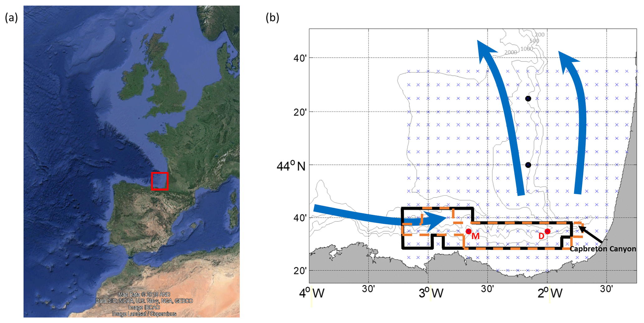
Figure 1(a) Location of the study area (red square). Map data © 2018 AND Data SIO, NOAA, U.S. Navy, NGA, GEBCO. Image IBCAO. Image: Landsat/Copernicus. (b) Close-up map of the study area. The winter IPC is represented by solid blue arrows. The grid used for the emulated HFR surface current fields is shown by blue crosses. The red dots provide the locations of the current vertical profiles that emulate the EuskOOS moorings: Matxitxako (red M) and Donostia (red D), whereas the black dots depict the location of the two extra moorings used for the 4-mooring scenario. The bold black lines delimit the winter reduced grid, whereas the dashed orange lines delimit the summer one. The grey lines show the 200, 500, 1000 and 2000 m isobaths.
The assessment of the performances of the data-reconstruction methods is carried out in terms of current velocities, using a model-based scenario based on the coastal observatory existing in the study area. Thus, the skills of two data-reconstruction methods are assessed and compared, aiming to give a first step towards their applicability for this specific case.
2.1 Assessment approach
The approach used for the analysis of the skills of the data-reconstruction methods is based on the use of a realistic numerical simulation as a true ocean, that provides both the emulated observations and the 3D reference field (hereinafter “reference field”) that will be used to assess the results of the 3D reconstruction. This is a well-established methodology inspired by the techniques used in observing system simulation experiments (OSSEs), and it is the only approach that allows us to quantify the skills of the data-reconstruction methods in the entire 3D domain considered for the reconstruction. The assessment approach consisted of three main steps (Fig. 2). First, the observations that emulate the data obtained from the EuskOOS platforms were extracted from a numerical simulation (for simplicity these “emulated observations” are called “observations” from here on). The extracted simulation data emulate the two vertical current profiles of the ADCPs located in the Matxitxako and Donostia moorings and the surface current fields of the HFR (see locations and coverage in Fig. 1b). Second, the two data-reconstruction methods were applied to the observations to compute the 3D reconstructed fields. Note that the ROOI method also uses historical data from a simulation to estimate the spatial covariances of the currents in the study area needed for the reconstruction. Finally, the 3D reconstructed fields (outputs of the methods) were compared to the reference field to assess the performances of the data-reconstruction methods.
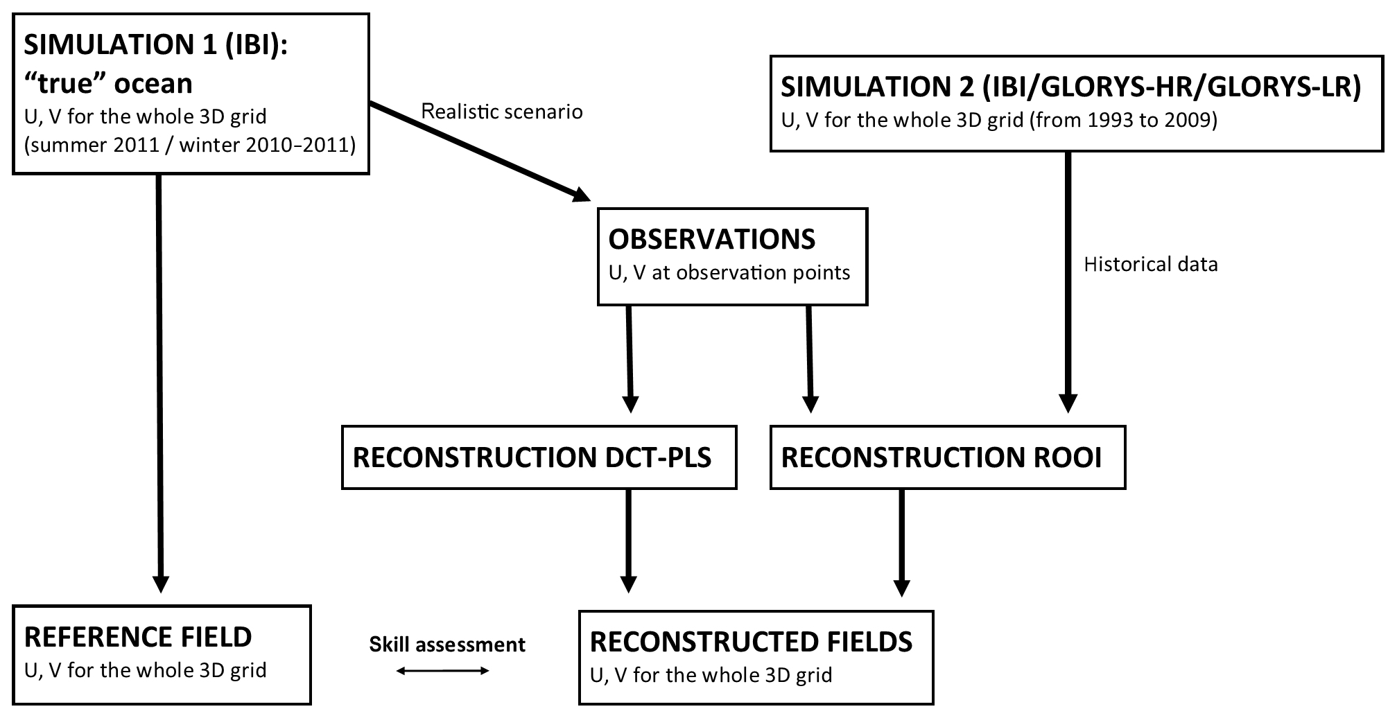
Figure 2Scheme of the approach used to test the performance of the two data-reconstruction methods described in Sect. 2.2. The models used for SIMULATION 1 and SIMULATION 2 are presented in Sect. 2.3.
Since the current regime is seasonally modulated, the performances of the two data-reconstruction methods were tested for winter and summer periods: November–December–January–February (2010–2011) and June–July–August–September (2011), respectively. The data-reconstruction methods were also analysed in a reduced grid case to evaluate the performance of the reconstructions in areas where the surface currents are highly correlated with the currents at the mooring locations (hereinafter called “well-sampled areas”). Since the moorings are located along the Spanish slope, where the zonal current velocity component (U) prevails over the meridional component (V), the reduced grid was determined only by the correlations obtained for this component (cross-correlation ≥0.8). This reduced grid mainly covers the Spanish slope area and slightly differs for the winter and summer periods (black and orange lines, respectively, in Fig. 1b).
A second scenario with two additional current vertical profiles along the French slope (see Fig. 1b) was also considered in order to assess the sensitivity of the data-reconstruction methods to different observational configurations (hereinafter called the “4-mooring scenario”).
2.2 Data-reconstruction methods
2.2.1 The ROOI method
The ROOI method was first proposed by Kaplan et al. (1997) to reconstruct sea surface temperatures (SSTs) from sparse data, and it has been applied since then for different variables such as sea level pressure (Kaplan et al., 2000), sea level anomalies (Church and White, 2006) or 3D velocity fields (Jordà et al., 2016). It is based on empirical orthogonal function (EOF) decomposition and the details can be found in Kaplan et al. (1997, 2000) or Jordà et al. (2016), so here only the basic elements are presented.
Expressing the 3D velocity field as a matrix Z(r, t), where r is the m vector of spatial locations and t the n vector of times, a spatial covariance matrix is first computed as . Then, an EOF decomposition can be applied:
where U is an m×m matrix whose columns are the spatial modes (EOFs), and Λ is the m×m diagonal matrix of eigenvalues. The velocity field can then be exactly reproduced as
in which the amplitude can be computed as α=UTZ.
In practice, the velocities at every grid point of the 3D analysis grid are not known, but only at a limited set of N locations (being N≪m). The problem we intend to solve is precisely that of retrieving the whole matrix Z from the available observations (e.g. surface velocities from HFR and velocity profiles at the ADCP locations). The first problem is that the eigenvector U and eigenvalue Λ matrices cannot be computed from actual observations (i.e. there are not enough samples), so a common choice is to use historical data from a realistic numerical simulation to represent the actual velocity statistics. A second aspect to be considered is that fitting high-order modes may introduce unwanted noise into the reconstruction. Thus, the Eq. (2) is truncated to include only the M leading EOFs, so that the contribution of the higher-order modes (accounting for local small-scale features) is neglected:
The next problem is that obviously the amplitudes cannot be obtained as in Eq. (2), since now we do not know Z. Instead, the M amplitudes can be determined under the constraint that the reconstructed ZM fits the observations available at each time step. More generally, the amplitudes are obtained by minimizing a cost function that takes into account the observational noise and the role of neglected modes (see Kaplan et al., 1997, 2000, for the complete derivation).
In summary, using the ROOI, the values of the velocity at every grid point of a predefined 3D grid can be obtained by merging the spatial modes of variability computed from a realistic numerical simulation (used as historical data) and the temporal amplitudes obtained using the available observations. Several sensitivity tests have been performed to tune the method and finally 20 modes have been considered (M=20). Regarding the spatial modes of variability, they have been obtained from different numerical simulations (see Sect. 2.3) to test the sensitivity of the results to the accuracy in the definition of the spatial covariances.
Table 1Details of the numerical simulations used in this study. Note that TS represents temperature salinity. (All URLs in this table were last accessed on 16 April 2020.)
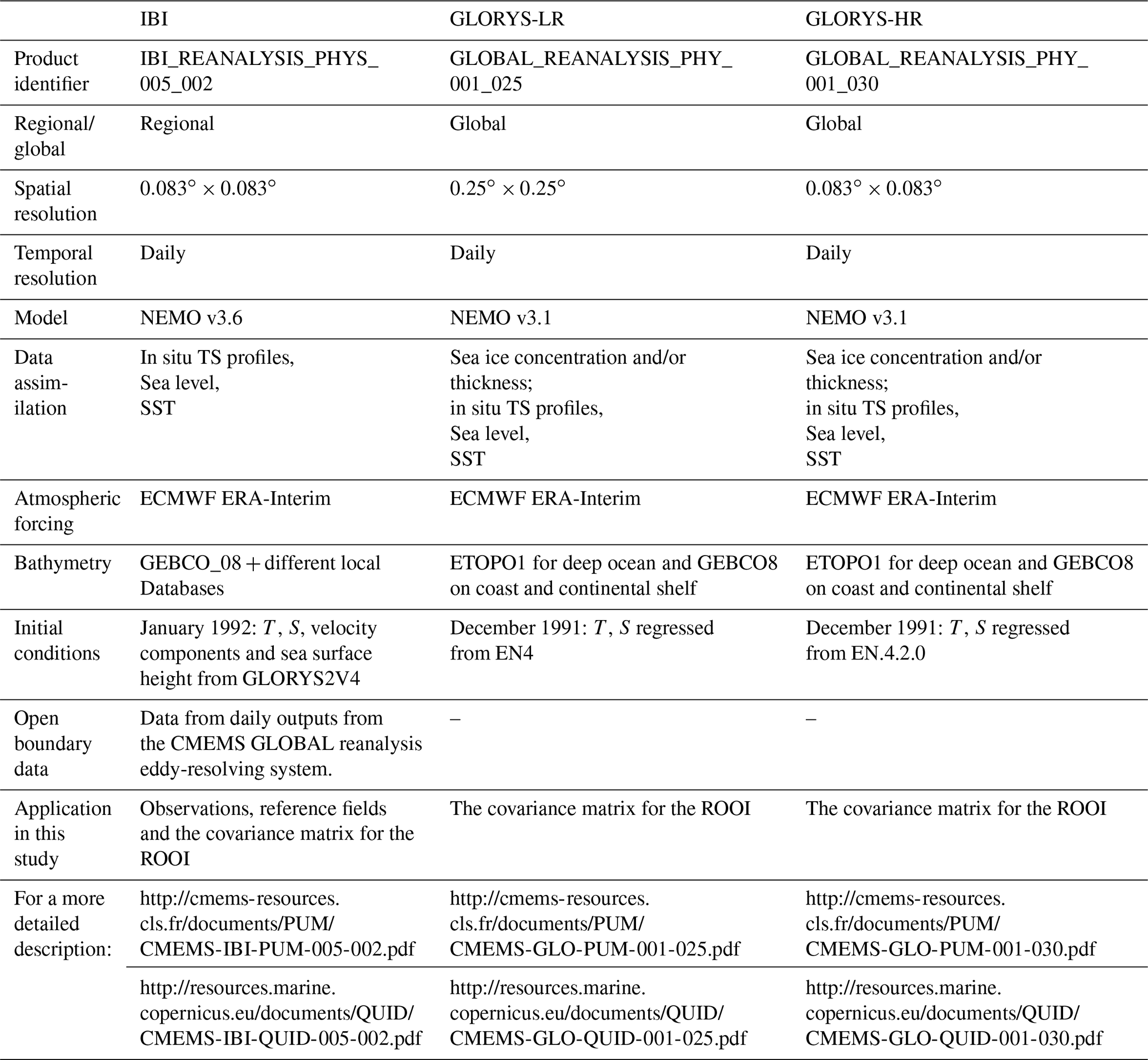
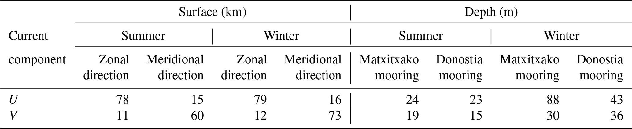
Table 2Seasonal spatial correlation length scales for the emulated current velocity components U and V in the study area, for the summer and winter periods and in zonal and meridional directions. Note that the surface horizontal scales are shown in kilometres and that the vertical scales in depth at Matxitxako and Donostia mooring points are shown in metres.
2.2.2 The DCT-PLS method
The DCT-PLS method is a straightforward technique proposed by García (2010), based on a penalized least square regression. Fredj et al. (2016) showcased the method's skills for the 2D reconstruction of HFR surface current fields along the mid Atlantic coast of the United States with high accuracy. In this section the basic principle of the method is explained; however, for more details the reader is referred to García (2010) or Fredj et al. (2016).
The main aim of the method is to find the best fitting model, which is based on discrete cosine transforms (DCTs) and one smoothing (fitting) parameter s. Thus, the fitting model that corresponds to each s is tested by cross-validation in order to obtain the best one. The general approach of the method is as follows: for each s (i.e. for each fitting model), the observations are split into two subsets: the training set, which is used to fit the model, and the test set, which is used to test it. This test is carried out by the trade-off (F) between the bias of the fitting (residual sum of squares, RSS) and the variance of the results of the created model (penalty term P):
where y is the data of the test set, is the data of the created model and D is a second-order difference derivative. Then, for the same s, this procedure is repeated for different training and test sets obtaining different F values at each time. The mean value of F (that is, E[F]) will provide a general cross-validation (GCV) score that corresponds to each fitting model (i.e. to each s):
and the best fitting model will be the one that minimizes the GCV score:
In conclusion, here we introduce a penalized least square method, based on discrete cosine transforms, with one smoothing parameter approach consisting of minimizing a criterion that balances the fidelity with the current data, measured by the RSS, and a P that reflects the noisiness of the smooth current data.
2.3 Numerical simulations
The Atlantic–Iberian Biscay Irish simulation, and particularly the IBI_REANALYSIS_PHYS_005_002 product (hereinafter IBI), provided by the Copernicus Marine Environment Monitoring Service (CMEMS), was used to obtain the true ocean from which the observations and the reference field were extracted, as explained in Sect. 2.1. The IBI reanalysis is based on a realistic configuration of the NEMO model for the Iberian Biscay Irish region (Fig. 1a), which assimilates in situ and satellite data. For more details, see Table 1; a complete description of the product and its validation can be found in Sotillo et al. (2015) and the links shown in Table 1. In Sect. 3, the realism of IBI simulations is assessed based on previous knowledge of the circulation in the area and used to provide an overview of the dynamical characteristics of the study area to support the discussion of the results.
The spatial covariances required for the ROOI have been obtained from IBI and two additional numerical simulations (see Fig. 2) with daily outputs from 1993 to 2009, with the objective of exploring the impact on the reconstruction of an imperfect definition of the covariances. The two additional numerical simulations used for this purpose were the GLORYS high-resolution (GLOBAL_REANALYSIS_PHY_001_030 product, hereinafter called ”GLORYS-HR”) and the low-resolution (GLOBAL_REANALYSIS_ PHY_ 001_025 product, hereinafter called “GLORYS-LR”) reanalyses. The general details of these products are listed in Table 1, along with links to additional information about the products and their validation. Thus, the ROOI method was tested both in an optimal configuration, where the covariance matrix was obtained from the same numerical simulation used as the reference field (i.e. IBI), and in two suboptimal configurations: one in which the covariances were obtained from a high-resolution numerical simulation (i.e. GLORYS-HR), which is supposed to capture the same range of processes as IBI although not exactly, and another one from a low-resolution numerical simulation (i.e. GLORYS-LR), which differs from IBI in the numerical code and also in the resolvable spatial scales.
The same 3D grid was considered for the reference field, the covariance matrices, and to extract the observations at the surface layer or in the vertical profiles at the grid points closest to the mooring locations (Fig. 1b). The horizontal grid spacing was given by the native horizontal grid of IBI and GLORYS-HR (1∕12∘) (Fig. 1b). Thus, for the computation of the covariance matrices with GLORYS-LR, the data were linearly interpolated to the IBI grid points. The vertical configuration was adapted to the levels of the real ADCPs with data every 8 m (from −12 to −148 m). Since the surface layer was set at −0.5 m, all the used numerical simulation fields were linearly interpolated to this vertical configuration (i.e. −0.5, −12, −20, −28, … −148 m).
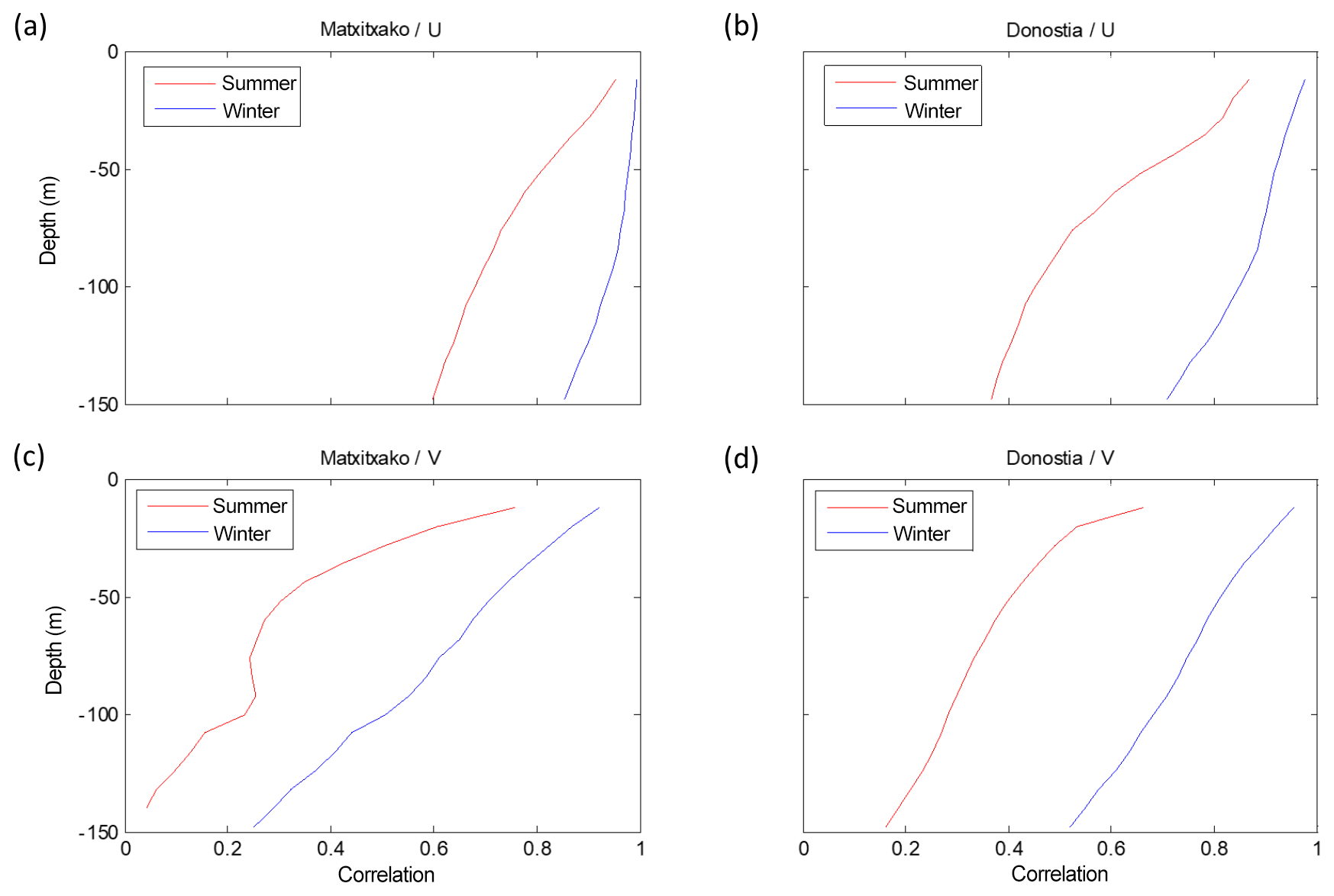
Figure 3U (a, b) and V (c, d) temporal cross-correlations between the surface and the water column levels for winter (blue) and summer (red) periods. In the Matxitxako location (a, c) and in the Donostia location (b, d).
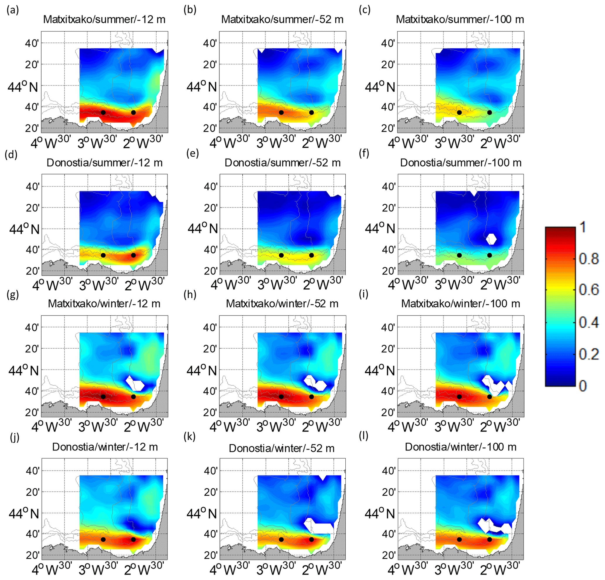
Figure 4Temporal cross-correlation maps between the water column levels considered and the surface points of the HFR grid for U. (a, b, c, g, h, i) for the Matxitxako mooring and (d, e, f, j, k, l) for the Donostia mooring. Different depths are considered: −12 m (a, d, g, j), −52 m (b, e, h, k) and −100 m (c, f, i, l), for summer (a–f) and winter (g–l). The white gaps are the areas where the confidence level is less than 95 %. The black dots depict the locations of the current vertical profiles.

Figure 5Temporal cross-correlation maps between the water column levels considered and the surface points of the HFR grid for V. (a, b, c, g, h, i) for the Matxitxako mooring and (d, e, f, j, k, l) for the Donostia mooring. Different depths are considered: −12 m (a, d, g, j), −52 m (b, e, h, k) and −100 m (c, f, i, l), for summer (a–f) and winter (g–l). The white gaps are the areas where the confidence level is less than 95 %. The black dots depict the locations of the current vertical profiles.
2.4 Skill assessment
The skills of the data-reconstruction methods were assessed by means of the root-mean-square difference (RMSD) between the reconstructed fields (x) and the reference fields (y). The RMSDs were computed at each point of the 3D grid for each study period and for U and V. Thus, for one grid point and N time steps,
where xt and yt are the reconstructed and reference fields at each time step, respectively.
The relative RMSD, relative to the root-mean-square (rms) current (hereinafter RRMSD), was also considered, since the strength and variability of the current are different at different locations of the study area and therefore influence the magnitude of the RMSDs. Therefore, the considered relative value is
where
Since RMSD and RRMSDs were computed for each study period and for each velocity component, hereinafter we use RMSD-U and RRMSD-U as RMSD and RRMSD computed for U and RMSD-V and RRMSD-V as RMSD and RRMSD computed for V. When the RRMSD is equal to 1 at one point for a study period, it means that the RMSD equals the rms of the studied period at that point.
In this section, the characteristics of the simulated IBI currents are validated against those found in previous studies based on real HFR and ADCP data (e.g. Rubio et al., 2013, 2019; Solabarrieta et al., 2014). We focus on the comparison of the statistical properties (i.e. spatio-temporal correlations), which are also the basis for the reconstruction methods, and, in particular, on the spatial correlation length scales and temporal cross-correlations (see Appendix A for a detailed description of the computation of the correlations). The main aim is to provide an overview of the currents used to test the data-reconstruction methods as ground information in order to justify the scenarios and to support the discussion on the performances of the data-reconstruction methods. Indeed, the best performances are expected in the areas and periods of higher cross-correlation between currents at different locations and vertical levels.
As shown in Table 2, the spatial correlation length scales along the water column are higher for U than for V, since the profiles of both moorings are located in the Spanish slope, where the slope current prevails. Moreover, the highest correlation values are observed at Matxitxako, which is under a stronger influence of the slope current (Rubio et al., 2013; Solabarrieta et al., 2014). The scales are larger in winter than in summer when the water column is well mixed (Rubio et al., 2013, 2019). Regarding surface currents, the horizontal spatial correlation length scales are higher for the along-slope velocity components when considering the same direction for the computation of the correlation (i.e. for U, correlation computed in the zonal direction along the Spanish coast and for V correlation computed along the meridional direction along the French coast). The highest horizontal spatial correlation length scales are observed along the Spanish coast, and the scales are slightly larger in winter than in summer. These results are coherent with the presence of the along-slope current in the area, which is stronger and more persistent in winter and along the Spanish coastal area (Solabarrieta et al., 2014).
Concerning the temporal cross-correlation, the same patterns shown by the spatial correlation length scales are observed. The temporal cross-correlation profiles between the surface and subsurface levels (Fig. 3) and the temporal cross-correlation maps (Figs. 4–5) show that the highest correlations are observed for the along-slope component of the current in winter (with maximum correlation along the vertical levels at Matxitxako), and that the decrease in the correlation with depth is sharper in summer.
It is worth highlighting that the model-based spatial correlation length scales and temporal cross-correlations are coherent with those obtained from real observations (Rubio et al., 2019; see also Sect. S1 in the Supplement), validating the use of IBI to emulate the study case of the SE-BoB observatory.
Table 3Summary of the results of the reconstructions with ROOI (with GLORYS-LR) and DCT-PLS in terms of spatial mean RMSDs and RRMSDs for the entire and reduced grids, the summer and winter study periods, and different depths.
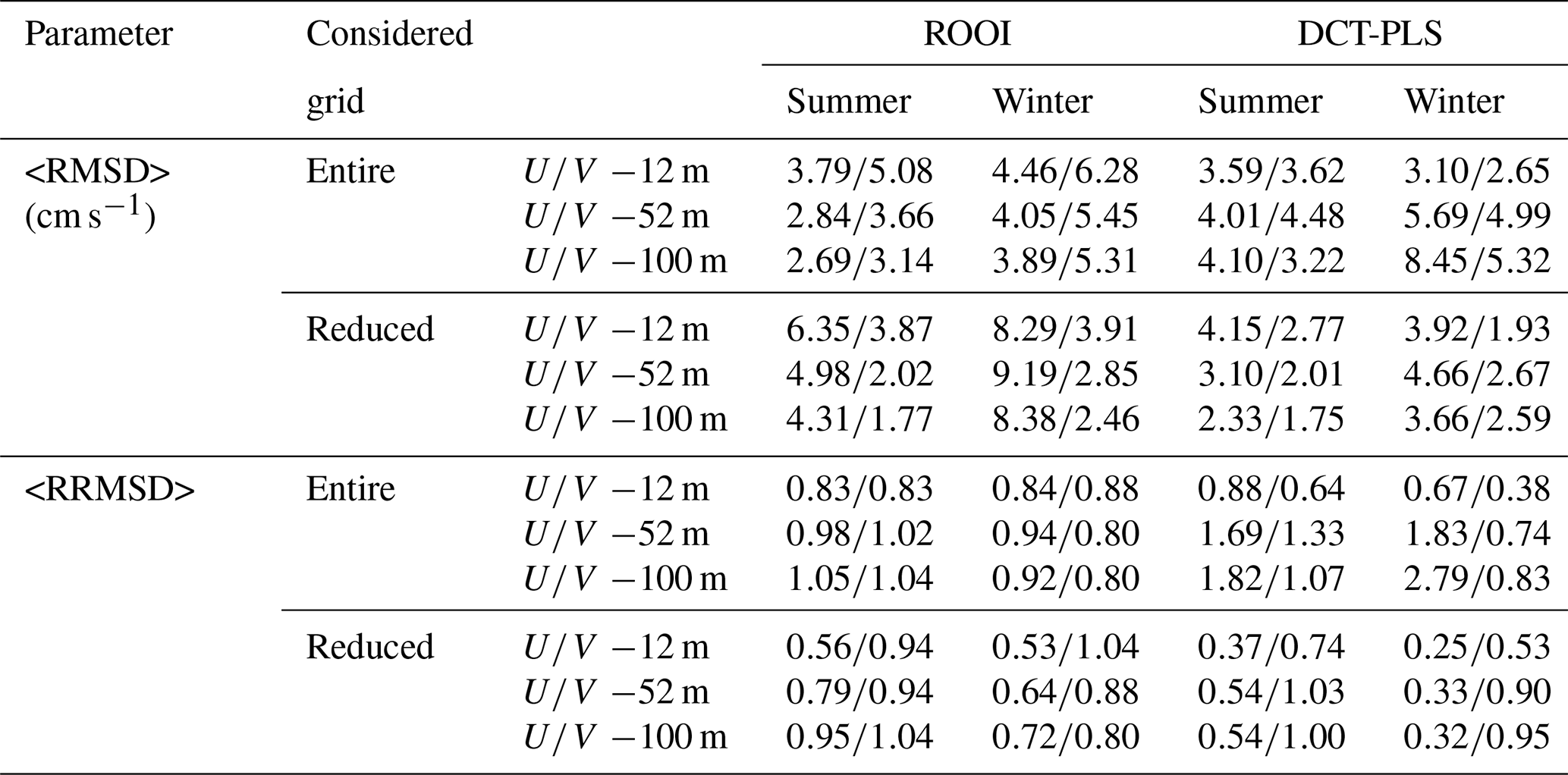
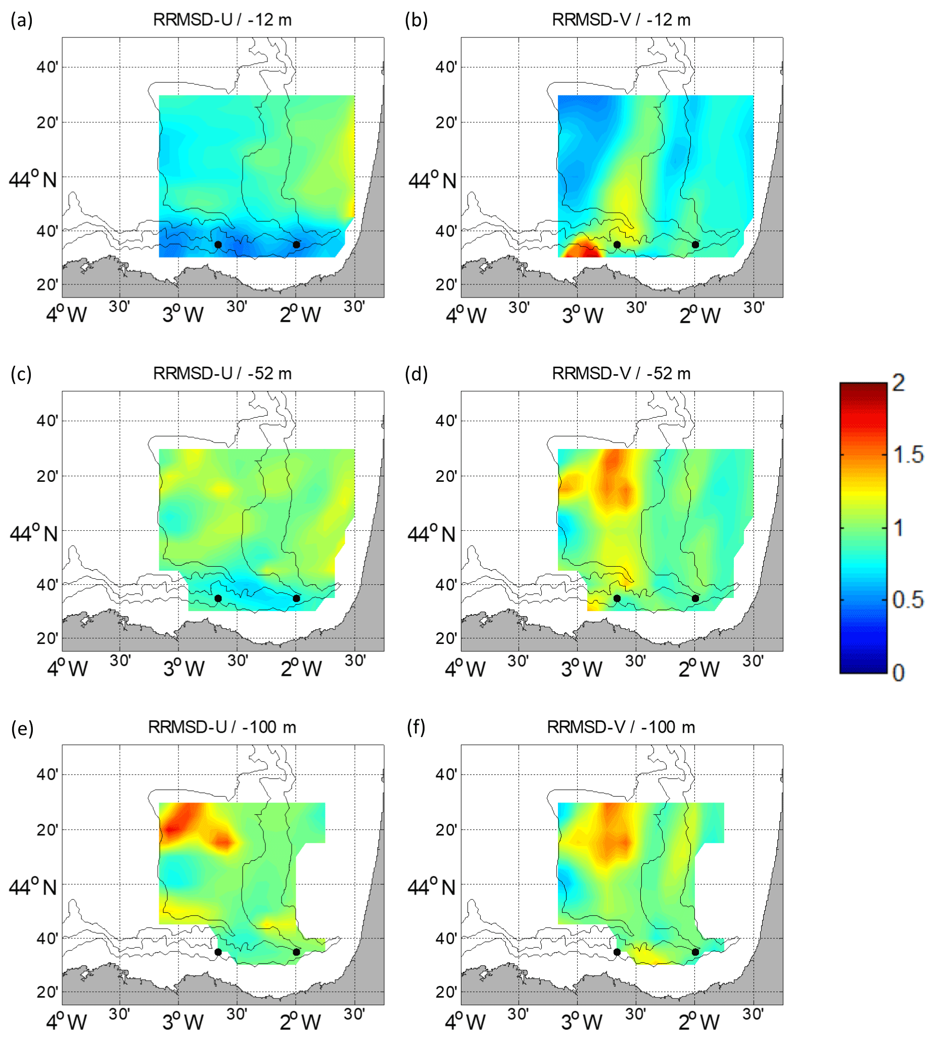
Figure 6RRMSD maps for the summer period between the reference fields and the outputs of the ROOI with GLORYS-LR for U (a, c, e) and V (b, d, f). Different depths are considered: −12 m (a, b), −52 m (c, d) and −100 m (e, f). The black dots depict the locations of the current vertical profiles.
4.1 Data reconstruction
The results, in terms of RMSDs and RRMSDs, are summarized in Table 3. It is observed that the RMSDs and the RRMSDs are affected by the spatial and temporal variability of the slope current regime. The mean RMSDs are, in general, higher in winter than in summer due to more intense currents in that period. However, the rms values are also higher and in relative terms the reconstructions show, overall, better results in winter (lower mean RRMSDs). This dependence of the results on the current regime can be also observed if we compare the reduced and the entire grid cases. For the reduced grid case, that covers an area of intense zonal slope currents, highest mean RMSDs and lowest mean RRMSDs are generally obtained for U. Since V is much weaker for this grid, it provides the lowest mean RMSDs. Nevertheless, the expected increase in the mean RRMSDs is not so clear compared to the entire grid case due to lower rms values.
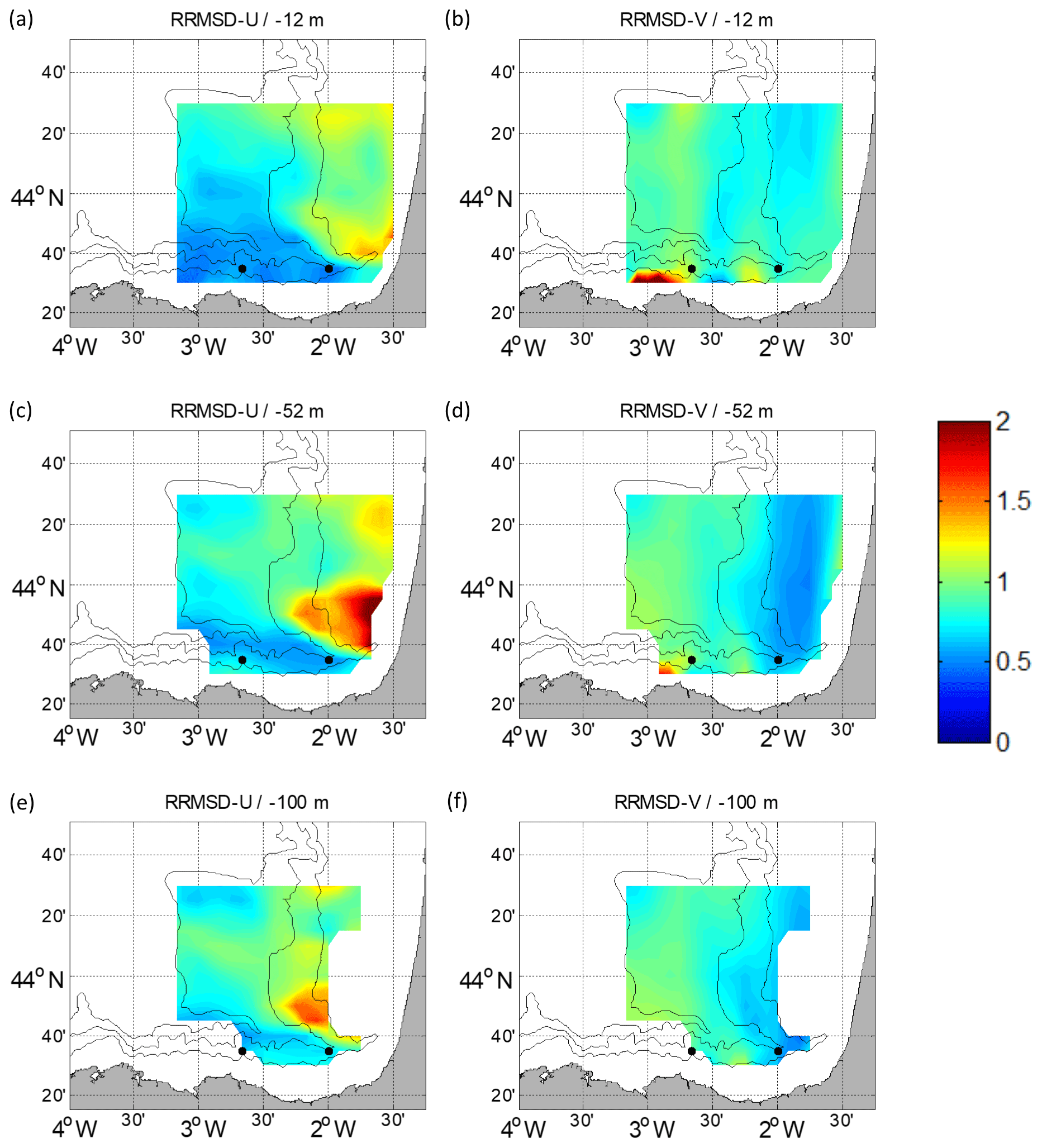
Figure 7RRMSD maps for the winter period between the reference fields and the outputs of the ROOI with GLORYS-LR for U (a, c, e) and V (b, d, f). Different depths are considered: −12 m (a, b), −52 m (c, d) and −100 m (e, f). The black dots depict the locations of the current vertical profiles.
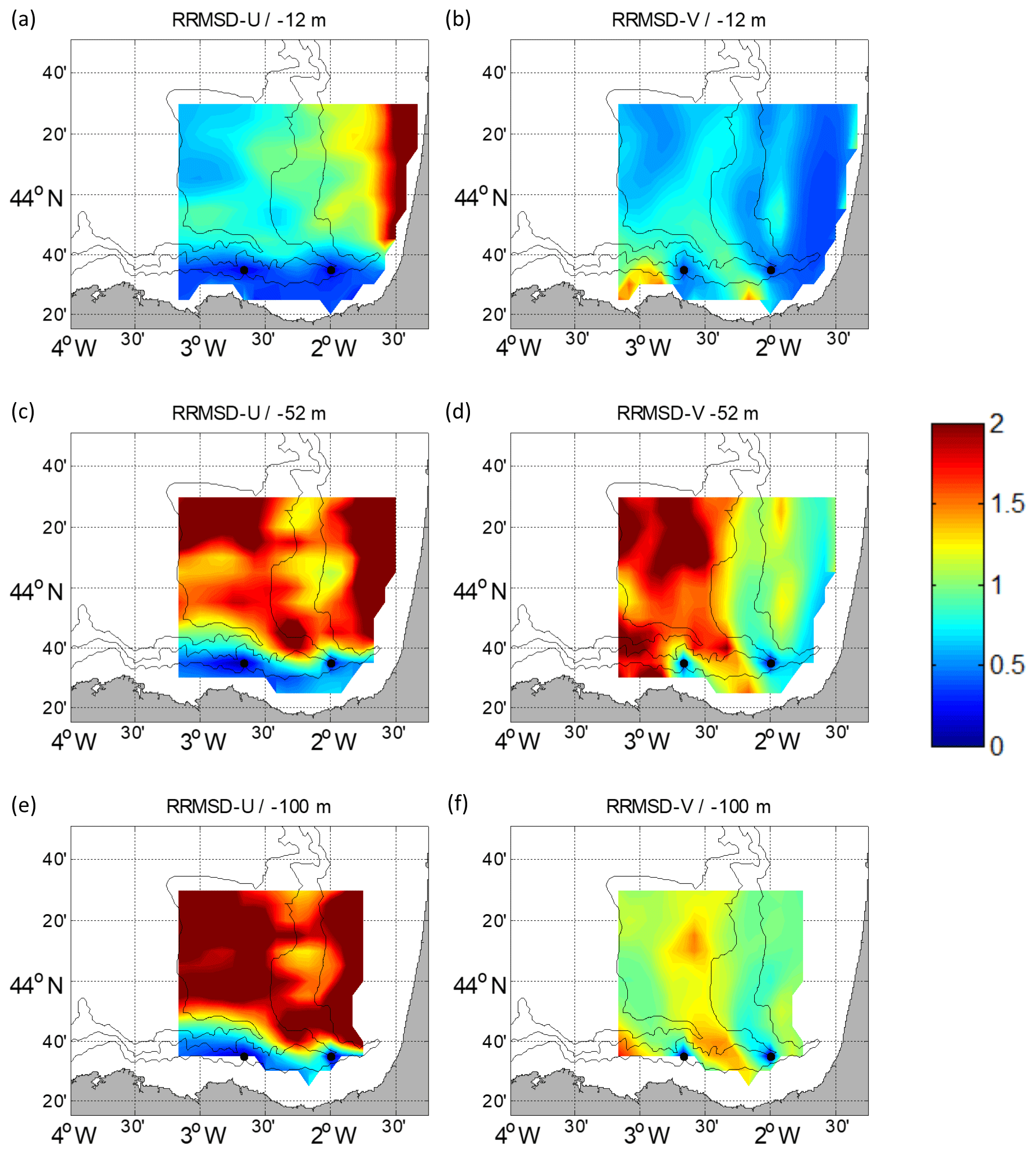
Figure 8RRMSD maps for the summer period between the reference fields and the outputs of the DCT-PLS for U (a, c, e) and V (b, d, f). Different depths are considered: −12 m (a, b), −52 m (c, d) and −100 m (e, f). The black dots depict the locations of the current vertical profiles.
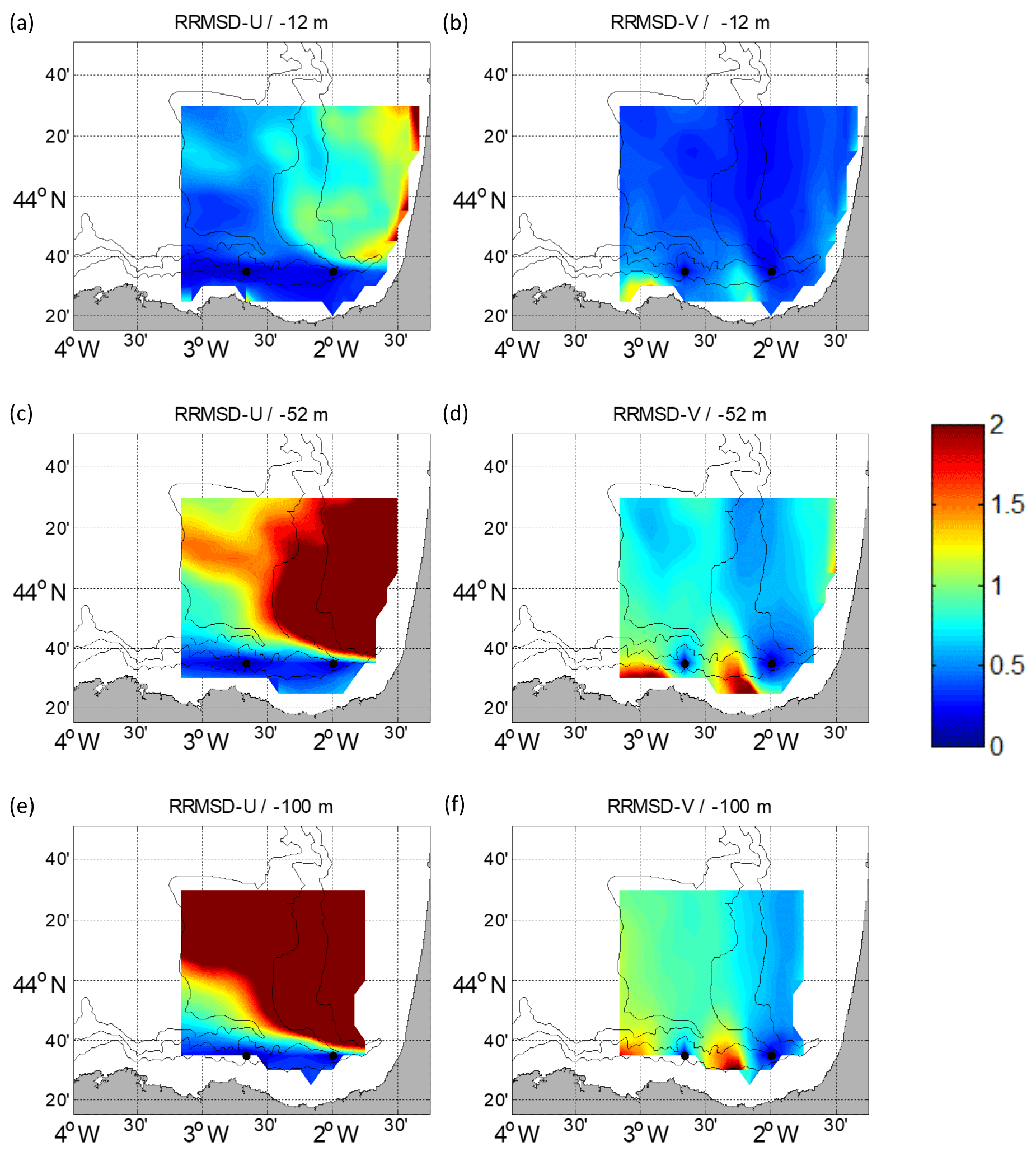
Figure 9RRMSD maps for the winter period between the reference fields and the outputs of the DCT-PLS for U (a, c, e) and V (b, d, f). Different depths are considered: −12 m (a, b), −52 m (c, d) and −100 m (e, f). The black dots depict the locations of the current vertical profiles.
Regarding the comparison between data-reconstruction methods, for the entire grid case, the mean RRMSD-U values are remarkably higher for the DCT-PLS. Conversely, for the reduced grid case, the results for the RRMSD-U for the DCT-PLS are better. The mean RRMSD-V values do not show any specific trend. This shows that the DCT-PLS performs better in well-sampled areas, whereas the ROOI performs well also out of these areas.
All these results, in addition to more specific analyses, are shown below in terms of RRMSDs by means of maps (Figs. 6–9) and horizontal mean value profiles along the water column (Figs. 10–11). The results of the RMSDs are shown in Sect. S4. For the ROOI RRMSD maps, the results with the spatial covariances from GLORYS-LR are the ones presented in Figs. 6–7, because those are the ones that most challenge the method. In fact, for the ROOI with GLORYS-HR, the RRMSDs are even lower (see Sect. S2), with the main conclusions being very similar.
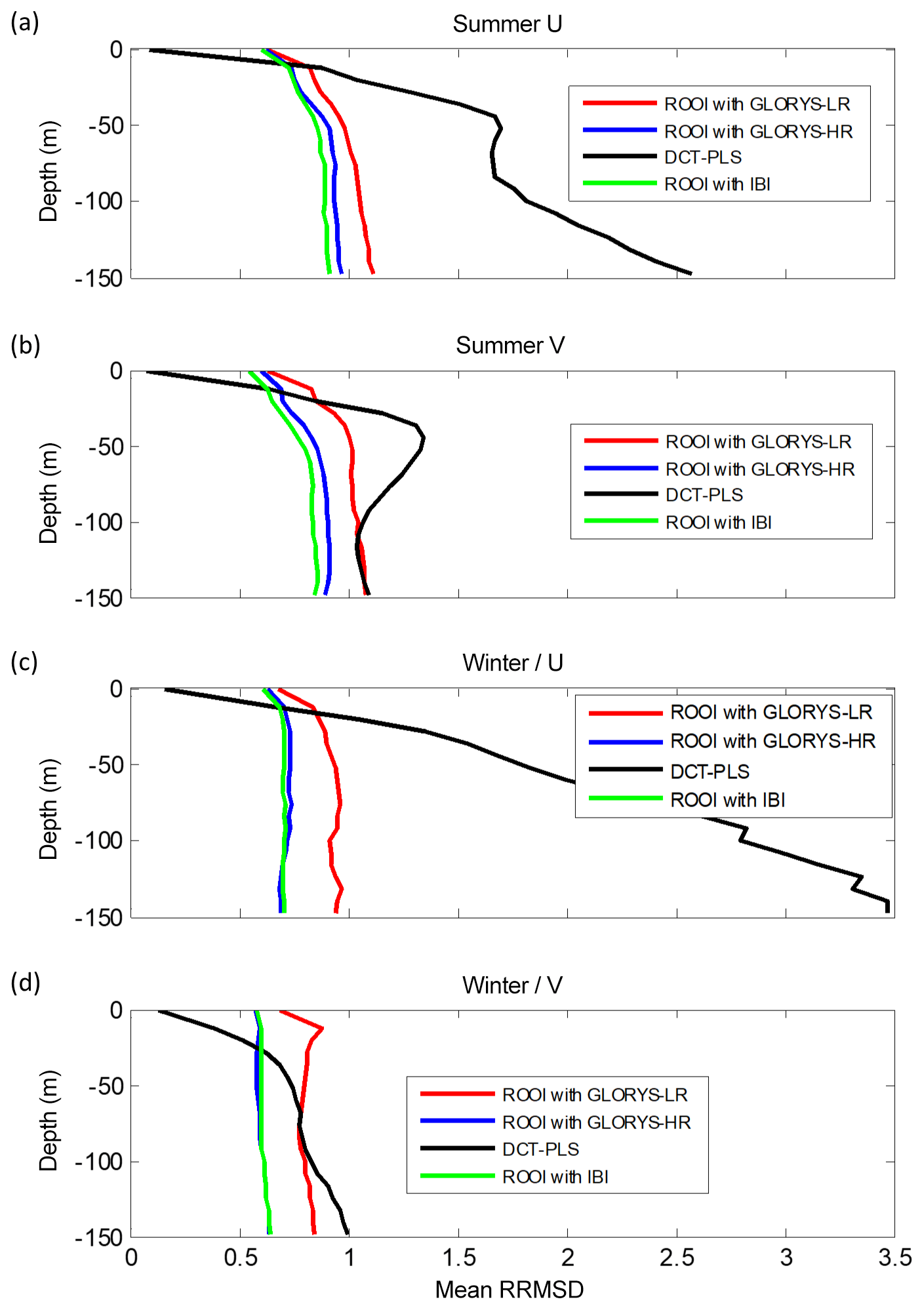
Figure 10Mean RRMSDs related to all the data-reconstruction methods for each depth considering the entire grid for the summer period (a, b) and for the winter period (c, d). U is shown in (a, c) and V in (b, d).
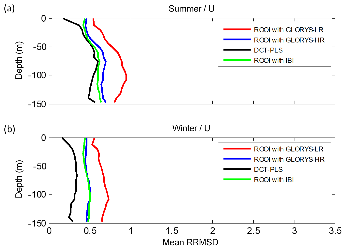
Figure 11Mean RRMSD-U related to all the data-reconstruction methods for each depth considering the reduced grid domain for the summer period (a) and for the winter period (b).
For the ROOI, the RRMSD spatial distribution is more uniform in summer (Fig. 6) than in winter (Fig. 7) due to the more variable summer current regime. The Spanish slope area shows the lowest RRMSD-Us due to the strong signal of the along-slope current, with lower values in winter than in summer. This suggests that the reconstructed fields are more accurate in well-sampled areas and that U is well resolved in the numerical simulations used for the definition of the spatial covariances. For the RRMSD-V, the French slope and part of its platform show the lowest values in winter, indicating that the slope current is well reconstructed for that period. Since the density of the observations is much higher at the surface, it is expected that the method performs better in the upper layers; in fact, it is observed that the RRMSDs increase with depth. This increase is sharper in summer than in winter, probably due to higher vertical shear in the currents due to the stratification conditions. It is shown that for the ROOI with GLORYS-LR, the RRMSDs are, in general, below 1.25; that is, the RMSD is below 1.25 times the rms value at each point, except for some concrete areas.
Regarding the DCT-PLS, RRMSD maps (Figs. 8–9) show the lowest values near to the surface and the mooring locations, showing that this method works better in well-sampled areas. The RRMSDs are lower in winter (Fig. 9) than in summer (Fig. 8). For the RRMSD-U, the Spanish slope area shows the lowest values for both periods, whereas low RRMSD-Vs are observed over the French slope in winter, showing that this method is also able to reconstruct the slope current. Overall, RRMSDs increase with depth; nevertheless, in summer the RRMSD-Vs are higher for −52 m (Fig. 8d) than for −100 m (Fig. 8f). This could be related to a stronger vertical shear related to the seasonal thermocline, which in this period is located between −30 and −50 m. For the DCT-PLS, the RRMSDs are not as smooth as for the ROOI, with RMSDs near (off) the observation areas lower (higher) than half (twice) the rms value at each point.
Thus, for both methods, lower RRMSDs are observed in winter than in summer, along the slope for the along-slope component of the velocity and close to the surface. While the DCT-PLS is more effective at well-sampled areas, the ROOI performs better in the rest of the areas. In general, the best performances are located in the well-sampled areas (Figs. 3–5), showing that the a priori analysis, shown in Sect. 3, can provide an approximate idea about the areas where the reconstructions could, in principle, perform better.
It is observed that the results for the DCT-PLS worsen quickly as we get away from the observation points. Considering the −52 m depth layer, we observe that RRMSD values obtained with the DCT-PLS method increase from 0 to 0.25 at ∼31 km (6.3 km) for the U(V) component in the zonal (meridional) direction.
A further analysis of the spatial mean of the RRMSDs with depth (Figs. 10–11) is performed to evaluate the methods' skills, regardless of the spatial variability shown in previous figures. Note that the same grid points were considered for both data-reconstruction methods and that the ROOI with IBI, GLORYS-LR, and GLORYS-HR are shown in this analysis. The analysis was carried out in the entire grid and the reduced grid (see Fig. 1b) in order to explore the sensitivity of the results to the choice of different areas.
For the entire grid case (Fig. 10), the ROOI with GLORYS-LR provides similar results as the DCT-PLS for V (Fig. 10b and d), whereas it provides much better results for U (Fig. 10a and c). On the other hand, the ROOI with IBI and GLORYS-HR performs better for both velocity components. In addition, as it could be noticed in Table 3 and in Figs. 6–9, the mean RRMSDs show RMSDs around or less than 1 times the rms value at each point, except for U for the DCT-PLS.
In the reduced grid case (Fig. 11), the lowest mean RRMSD-Us are observed for the DCT-PLS, performing significantly better than the ROOI. In general, the mean RMSDs are around or less than 0.75 times the rms value at each point, with values around or less than 0.5 times the rms value for the DCT-PLS. This provides quite a satisfactory reconstruction of the along-slope velocity component in the Spanish slope area. Thus, if the whole water column is considered, the ROOI provides again smaller RRMSDs than the DCT-PLS for the entire grid case, whereas the DCT-PLS provides better results in well-sampled areas.
With regard to the seasonal analysis, lower RRMSDs are observed in winter (Figs. 10–11). The only exception is the RRMSD-U in the entire grid case for the DCT-PLS (Fig. 10a and c) due to the high RRMSDs over the French shelf and slope for that period (see Sect. S3), since this method expands the zonal component to that area of meridional regime.
Considering all the analysed depths and study periods, satisfactory reconstructions are obtained by both methods. These reconstructions provide mean RMSDs for each depth (Figs. 10–11) ranging from 0.55 (0.7) cm s−1 to 10.94 (9.58) cm s−1 for the entire (reduced) grid and mean RRMSDs ranging from 0.07 (0.12) to 3.47 (1.31) with typical values around 1 or less, i.e. with reconstructed field errors around the rms value or less at each point. In general, the RRMSDs are increased with depth and thus RMSDs up to 10.94 cm s−1 are obtained at −150 m.
4.2 Sensitivity test: increased number of ADCPs
An analysis with two additional ADCPs was carried out in order evaluate the sensitivity of the data-reconstruction methods to an increased number of observations. The two extra ADCPs were located over the French slope, since this could be a strategic area to monitor the winter slope current downstream of the Capbreton Canyon.
Only the winter period is shown, when the slope current is the strongest and the effects of the new scenario are more noticeable. Also, we show here the results obtained for the −52 m layer, due to its representativeness of the entire water column. The performance of the data-reconstruction methods for this configuration is assessed by subtracting the RRMSD maps of the 2-mooring case to the 4-mooring case. Therefore, the negative (positive) values in Fig. 12 show that the RRMSD is lower (higher) for the 4-mooring configuration, thus showing a better (worse) performance. In general, in this new scenario the performance of both data-reconstruction methods improves, with smoother changes for the ROOI, since it already uses historical information of the covariances in the whole study area.

Figure 12The 4-mooring scenario RRMSD maps subtracted by the 2-mooring scenario RRMSD maps for winter at −52 m. Negative values mean a better performance in the 4-mooring scenario for U (a, b) and for V (c, d) for the ROOI (a, c) and for the DCT-PLS (b, d). The black dots depict the locations of current vertical profiles.
For U, the addition of two extra ADCP profiles does not affect the Spanish slope area where there are already two moorings that capture the slope current. In the rest of the grid, for the DCT-PLS (Fig. 12b), the performance of the reconstruction is remarkably improved; whereas, for the ROOI (Fig. 12a), although in general the reconstruction is improved, there are some specific areas where the RRMSD-Us are slightly increased. For V, the results improve along the French slope, which are more remarkable for the DCT-PLS (Fig. 12d). However, for this method, the RRMSD-Vs are increased in the areas close to that slope, probably due to the spread of the information from the slope observations to those nearby areas which are not affected by the slope current regime.
In this paper we investigated the feasibility of combining data from multiplatform observing systems to reconstruct 3D velocity fields in the SE-BoB by means of two data-reconstruction methods. More precisely, we assessed the performance of such methods in the case of combining surface current data (as the ones provided by a long-range HFR system) and current vertical profiles (as the ones provided by two moorings equipped with ADCPs) in an emulated scenario based on an existing observatory (being also a typical configuration that can be found in other coastal areas). The performances of the methods were assessed through a classical approach conceptually similar to OSSEs, where a realistic simulation was regarded as the true ocean. This assessment approach allowed for the comprehensive evaluation of the selected methods as a first step towards their application to real data in the study area. Besides, it provides a best-practice methodology for the evaluation of the challenges and limitations of this kind of method in a broader way, prior to their applications to real data in other study cases. An interesting further step, out of the scope of the present paper, would be to evaluate the robustness of the reconstruction methods for different observational errors.
We obtained satisfactory reconstruction results with spatial mean RMSDs typically ranging between 0.55 and 7 cm s−1, for the first 150 m depth, with mean relative errors of 0.07–1.2 times the rms current at each point for most of the cases. The main feature of the region, the slope current, was well reconstructed by both methods, and it significantly improved when the information of two additional moorings was used for the reconstruction.
Regarding the data-reconstruction methods, each one has its pros and cons. The DCT-PLS is only fed with the observations with no extra information about the study area, so its configuration is simpler. It performs well in well-sampled areas, but its quality is quickly degraded elsewhere. On the other hand, the ROOI is a robust data-reconstruction method that uses additional historical information, and thus provides better results in undersampled areas. The shortcoming of this method is that it needs accurate historical information of the study area. This is typically obtained from a realistic numerical simulation of the region, although it does not need to be contemporary to the observational period (i.e. from a hindcast simulation). Also, the method requires more tuning, so its implementation demands a careful testing of the parameters.
The tested methods have proven to be reliable, showing that it would be feasible to use them to reconstruct 3D current fields in the study area. In addition, they also could be used in a wide range of applications, due to their low computational cost. As, for instance, to obtain new operational products, combining data from different sources and complementary spatial coverage in near real time. Moreover, through OSSEs and observing system experiments (OSEs), an optimization of existing observing networks can be proposed, providing a potential decision-making tool for future planning of coastal observatories or to set up optimal operational data assimilation strategies. The use of these methods can be an alternative to data assimilation approaches (more expensive computationally and more complex to set up) as far as they do not require users to run a numerical model. This is especially appealing for the marine rapid environmental assessment (MREA). The 3D reconstructed velocity fields can also be used for model validation, as well as for broadening the utility of coastal observing systems to biological, geochemical and environmental issues.
The correlation (R) between two variables x1 and x2 is defined as follows:
where μi is the mean value of xi, i.e. μi=E[xi]. In this study, the correlation was used to estimate the relationships between the emulated horizontal currents in two different ways: by means of spatial relationships, determined by spatial correlation length scales (horizontal and vertical), and by means of temporal relationships, determined by temporal cross-correlations between two different points for a certain period of time. Note that for all the correlations presented here the confidence level considered is 95 %.
The spatial correlation length scales are the maximum distances between the grid points where the currents can be considered that are related. These scales were calculated for each velocity component, considering meridional and zonal directions for the computation by means of the e-folding method (described in Ha et al., 2007). If we consider one grid, one velocity component and one direction for the computation we can obtain one R value for each fixed distance between the grid points. That is, if we consider the zonal direction and the U component, x1 will be the value of U at each grid point and x2 will be the value of U at the grid point that is at a fixed distance away (a certain number of grid points in the zonal direction) from the grid point where x1 is evaluated. Therefore, we will obtain one R value for a fixed distance. Then, R is estimated for all the possible distances, thus obtaining correlation values depending on the distance between the grid points. This operation can be repeated for different time steps through a time period, obtaining a correlation vs. distance profile for each time step. All these profiles are then averaged for the time period that interests us, obtaining an averaged correlation vs. distance profile. In order to determine the spatial correlation length scale, as explained in Ha et al. (2007), a cut-off point is assumed in the averaged profile where the correlation coefficient decrease to e−1 times its original value.
Regarding the temporal relationships, the temporal cross-correlation is defined as the correlation of a variable (or two different variables) between two different points of a grid for a period of time, i.e. the correlation value R between a variable at one point (x1) and a variable at another point (x2) throughout the period of time analysed.
The IBI_REANALYSIS_PHYS_005_002 product is available on the CMEMS website (http://marine.copernicus.eu/services-portfolio/access-to-products/?option=com_csw&view=details&product_id=IBI_REANALYSIS_PHYS_005_002, CMEMS, 2020a).
The GLOBAL_REANALYSIS_PHY_001_025 product is available on the CMEMS website (http://marine.copernicus.eu/services-portfolio/access-to-products/?option=com_csw&view=details&product_id=GLOBAL_REANALYSIS_PHY_001_025).
The GLOBAL_REANALYSIS_PHY_001_030 product is available on the CMEMS website (http://marine.copernicus.eu/services-portfolio/access-to-products/?option=com_csw&view=details&product_id=GLOBAL_REANALYSIS_PHY_001_030, CMEMS, 2020b).
The supplement related to this article is available online at: https://doi.org/10.5194/os-16-575-2020-supplement.
IMN, EF, GJ, MB, AG, AC and AR contributed to the main structure and contents. In addition, IMN produced the figures, and EF and GJ provided the software and the tools and gave advice for the reconstruction with the DCT-PLS and ROOI methods, respectively.
The authors declare that they have no conflict of interest.
This article is part of the special issue “Coastal marine infrastructure in support of monitoring, science, and policy strategies”. It is not associated with a conference.
We thank the Emergencies and Meteorology Directorate – Security department – Basque Government for public data provision from the Basque Operational Oceanography System EuskOOS. This study has also been undertaken with the financial support of the Department of Environment, Regional Planning, Agriculture and Fisheries of the Basque Government (Marco Program). Ivan Manso-Narvarte was supported by a PhD fellowship from the Department of Environment, Regional Planning, Agriculture and Fisheries of the Basque Government. This study has been conducted using EU Copernicus Marine Service information. This is contribution number 962 of the Marine Research Division of AZTI-Tecnalia.
This research has been supported by the H2020 European Research Council (JERICO-NEXT (grant no. 654410)).
This paper was edited by George Petihakis and reviewed by three anonymous referees.
Barrick, D.: First-order theory and analysis of MF/HF/VHF scatter from the sea, IEEE T. Antenn. Propag., 20, 2–10, https://doi.org/10.1109/TAP.1972.1140123, 1972.
Broche, P., Forget, P., De Maistre, J., Devenon, J., and Crochet, M.: VHF radar for ocean surface current and sea state remote sensing, Radio Sci., 22, 69–75, https://doi.org/10.1029/RS022i001p00069, 1987.
Chapman, R., Shay, L. K., Graber, H. C., Edson, J., Karachintsev, A., Trump, C., and Ross, D.: On the accuracy of HF radar surface current measurements: Intercomparisons with ship-based sensors, J. Geophys. Res.-Oceans, 102, 18737–18748, https://doi.org/10.1029/97JC00049, 1997.
Church, J. A. and White, N. J.: A 20th century acceleration in global sea-level rise, Geophys. Res. Lett., 33, L01602, https://doi.org/10.1029/2005GL024826, 2006.
Cianelli, D., Falco, P., Iermano, I., Mozzillo, P., Uttieri, M., Buonocore, B., Zambardino, G., and Zambianchi, E.: Inshore/offshore water exchange in the Gulf of Naples, J. Marine Syst., 145, 37–52, https://doi.org/10.1016/j.jmarsys.2015.01.002, 2015.
CMEMS: Atlantic-Iberian Biscay Irish- Ocean Physics Reanalysis, available at: http://marine.copernicus.eu/services-portfolio/access-to-products/?option=com_csw&view=details&product_id=IBI_REANALYSIS_PHYS_005_002, last access: 16 April 2020a.
CMEMS: Global Ocean Physics Reanalysis, available at: http://marine.copernicus.eu/services-portfolio/access-to-products/?option=com_csw&view=details&product_id=GLOBAL_REANALYSIS_PHY_001_030, last access: 16 April 2020b.
Davies, A. M.: On determining current profiles in oscillatory flows, Appl. Math. Model., 9, 419–428, https://doi.org/10.1016/0307-904X(85)90107-6, 1985a.
Davies, A. M.: On determining the profile of steady wind-induced currents, Appl. Math. Model., 9, 409–418, https://doi.org/10.1016/0307-904X(85)90106-4, 1985b.
Davies, A. M.: Three dimensional modal model of wind induced flow in a sea region, Prog. Oceanogr., 15, 71–128, https://doi.org/10.1016/0079-6611(85)90032-1, 1985c.
De Valk, C. F.: Estimation of 3-D current fields near the Rhine outflow from HF radar surface current data, Coast. Eng., 37, 487–511, https://doi.org/10.1016/S0378-3839(99)00040-X, 1999.
Fredj, E., Roarty, H., Kohut, J., Smith, M., and Glenn, S.: Gap filling of the coastal ocean surface currents from HFR data: Application to the Mid-Atlantic Bight HFR Network, J. Atmos. Ocean. Tech., 33, 1097–1111, https://doi.org/10.1175/JTECH-D-15-0056.1, 2016.
Frouin, R., Fiúza, A. F., Ambar, I., and Boyd, T. J.: Observations of a poleward surface current off the coasts of Portugal and Spain during winter, J. Geophys. Res.-Oceans, 95, 679–691, https://doi.org/10.1029/JC095iC01p00679, 1990.
Fujii, S., Heron, M. L., Kim, K., Lai, J.-W., Lee, S.-H., Wu, X., Wu, X., Wyatt, L. R., and Yang, W.-C.: An overview of developments and applications of oceanographic radar networks in Asia and Oceania countries, Ocean Sci. J., 48, 69–97, https://doi.org/10.1007/s12601-013-0007-0, 2013.
Gangopadhyay, A., Shen, C. Y., Marmorino, G. O., Mied, R. P., and Lindemann, G. J.: An extended velocity projection method for estimating the subsurface current and density structure for coastal plume regions: An application to the Chesapeake Bay outflow plume, Cont. Shelf Res., 25, 1303–1319, https://doi.org/10.1016/j.csr.2005.03.002, 2005.
Garcia, D.: Robust smoothing of gridded data in one and higher dimensions with missing values, Comput. Stat. Data An., 54, 1167–1178, https://doi.org/10.1016/j.csda.2009.09.020, 2010.
Ha, K.-J., Jeon, E.-H., and Oh, H.-M.: Spatial and temporal characteristics of precipitation using an extensive network of ground gauge in the Korean Peninsula, Atmos. Res., 86, 330–339, https://doi.org/10.1016/j.atmosres.2007.07.002, 2007.
Haynes, R. and Barton, E. D.: A poleward flow along the Atlantic coast of the Iberian Peninsula, J. Geophys. Res.-Oceans, 95, 11425–11441, https://doi.org/10.1029/JC095iC07p11425, 1990.
Ivonin, D. V., Broche, P., Devenon, J. L., and Shrira, V. I.: Validation of HF radar probing of the vertical shear of surface currents by acoustic Doppler current profiler measurements, J. Geophys. Res.-Oceans, 109, C04003, https://doi.org/10.1029/2003JC002025, 2004.
Jordà, G., Sánchez-Román, A., and Gomis, D.: Reconstruction of transports through the Strait of Gibraltar from limited observations, Clim. Dynam., 48, 851–865, https://doi.org/10.1007/s00382-016-3113-8, 2016.
Kaplan, A., Kushnir, Y., Cane, M. A., and Blumenthal, M. B.: Reduced space optimal analysis for historical data sets: 136 years of Atlantic sea surface temperatures, J. Geophys. Res.-Oceans, 102, 27835–27860, https://doi.org/10.1029/97JC01734, 1997.
Kaplan, A., Kushnir, Y., and Cane, M. A.: Reduced space optimal interpolation of historical marine sea level pressure: 1854–1992, J. Climate, 13, 2987–3002, https://doi.org/10.1175/1520-0442(2000)013<2987:RSOIOH>2.0.CO;2, 2000.
Le Cann, B. and Serpette, A.: Intense warm and saline upper ocean inflow in the southern Bay of Biscay in autumn–winter 2006–2007, Cont. Shelf Res., 29, 1014–1025, https://doi.org/10.1016/j.csr.2008.11.015, 2009.
Marmorino, G., Shen, C., Evans, T., Lindemann, G., Hallock, Z., and Shay, L. K.: Use of “velocity projection” to estimate the variation of sea-surface height from HF Doppler radar current measurements, Cont. Shelf Res., 24, 353–374, https://doi.org/10.1016/j.csr.2003.10.011, 2004.
O'Donncha, F., Hartnett, M., Nash, S., Ren, L., and Ragnoli, E.: Characterizing observed circulation patterns within a bay using HF radar and numerical model simulations J. Marine Syst., 142, 96–110, https://doi.org/10.1016/j.jmarsys.2014.10.004, 2014.
Paduan, J. D. and Graber, H. C.: Introduction to high-frequency radar: reality and myth, Oceanography, 10, 36–39, https://doi.org/10.5670/oceanog.1997.18, 1997.
Paduan, J. D. and Washburn, L.: High-frequency radar observations of ocean surface currents, Annu. Rev. Mar. Sci., 5, 115–136, https://doi.org/10.1146/annurev-marine-121211-172315, 2013.
Peliz, Á., Dubert, J., Haidvogel, D. B., and Le Cann, B.: Generation and unstable evolution of a density-driven eastern poleward current: The Iberian Poleward Current, J. Geophys. Res.-Oceans, 108, 3268, https://doi.org/10.1029/2002JC001443, 2003.
Pingree, R. and Le Cann, B.: Structure, strength and seasonality of the slope currents in the Bay of Biscay region, J. Mar. Biol. Assoc. UK, 70, 857–885, https://doi.org/10.1017/S0025315400059117, 1990.
Pingree, R. and Le Cann, B.: Three anticyclonic Slope Water Oceanic eDDIES (SWODDIES) in the southern Bay of Biscay in 1990, Deep-Sea Res., 39, 1147–1175, https://doi.org/10.1016/0198-0149(92)90062-X, 1992a.
Pingree, R. and Le Cann, B.: Anticyclonic eddy X91 in the southern Bay of Biscay, May 1991 to February 1992, J. Geophys. Res.-Oceans, 97, 14353–14367, https://doi.org/10.1029/92JC01181, 1992b.
Prandle, D.: The vertical structure of tidal currents, Geophys. Astro. Fluid, 22, 29–49, https://doi.org/10.1080/03091928208221735, 1982.
Prandle, D.: The fine-structure of nearshore tidal and residual circulations revealed by HF radar surface current measurements, J. Phys. Oceanogr., 17, 231–245, https://doi.org/10.1175/1520-0485(1987)017<0231:TFSONT>2.0.CO;2, 1987.
Prandle, D.: A new view of near-shore dynamics based on observations from HF radar, Prog. Oceanogr., 27, 403–438, https://doi.org/10.1016/0079-6611(91)90030-P, 1991.
Ren, L., Nash, S., and Hartnett, M.: Observation and modeling of tide-and wind-induced surface currents in Galway Bay, Water Science and Engineering, 8, 345–352, https://doi.org/10.1016/j.wse.2015.12.001, 2015.
Roarty, H., Cook, T., Hazard, L., George, D., Harlan, J., Cosoli, S., Wyatt, L., Fanjul, E., Terrill, E., Otero, M., Largier, J., Glenn, S., Ebuchi, N., Whitehouse, B., Bartlett, K., Mader, J., Rubio, A., Corgnati, L., Mantovani, C., Griffa, A., Reyes, E., Lorente, P., Flores-Vidal, X., Saavedra-Matta, K., Rogowski, P., Prukpitikul, S., Lee, S.-H., Lai, J.-W., Guerin, C.-A., Sanchez, J., Hansen, B., and Grilli, S.: The Global High Frequency Radar Network, Frontiers in Marine Science, 6, 164, https://doi.org/10.3389/fmars.2019.00164, 2019.
Rubio, A., Fontán, A., Lazure, P., González, M., Valencia, V., Ferrer, L., Mader, J., and Hernández, C.: Seasonal to tidal variability of currents and temperature in waters of the continental slope, southeastern Bay of Biscay, J. Marine Syst., 109, S121–S133, https://doi.org/10.1016/j.jmarsys.2012.01.004, 2013.
Rubio, A., Mader, J., Corgnati, L., Mantovani, C., Griffa, A., Novellino, A., Quentin, C., Wyatt, L., Schulz-Stellenfleth, J., and Horstmann, J.: HF radar activity in European coastal seas: next steps toward a pan-European HF radar network, Frontiers in Marine Science, 4, 8, https://doi.org/10.3389/fmars.2017.00008, 2017.
Rubio, A., Manso-Narvarte, I., Caballero, A., Corgnati, L., Mantovani, C., Reyes, E., Griffa, A., and Mader, J.: The seasonal intensification of the slope Iberian Poleward Current, in: Copernicus Marine Service Ocean State Report, J. Oper. Oceanogr., 3, 13–18, https://doi.org/10.1080/1755876X.2019.1633075, 2019.
Shen, C. Y. and Evans, T. E.: Surface-to-subsurface velocity projection for shallow water currents, J. Geophys. Res.-Oceans, 106, 6973–6984, https://doi.org/10.1029/2000JC000267, 2001.
Shen, C. Y. and Evans, T. E.: Dynamically constrained projection for subsurface current velocity, J. Geophys. Res.-Oceans, 107, 24-21–24-14, https://doi.org/10.1029/2001JC001036, 2002.
Shrira, V. I., Ivonin, D. V., Broche, P., and de Maistre, J. C.: On remote sensing of vertical shear of ocean surface currents by means of a Single-frequency VHF radar, Geophys. Res. Lett., 28, 3955–3958, https://doi.org/10.1029/2001GL013387, 2001.
Solabarrieta, L., Rubio, A., Castanedo, S., Medina, R., Charria, G., and Hernández, C.: Surface water circulation patterns in the southeastern Bay of Biscay: new evidences from HF radar data, Cont. Shelf Res., 74, 60–76, https://doi.org/10.1016/j.csr.2013.11.022, 2014.
Sotillo, M., Cailleau, S., Lorente, P., Levier, B., Aznar, R., Reffray, G., Amo-Baladrón, A., Chanut, J., Benkiran, M., and Alvarez-Fanjul, E.: The MyOcean IBI Ocean Forecast and Reanalysis Systems: operational products and roadmap to the future Copernicus Service, J. Oper. Oceanogr., 8, 63–79, https://doi.org/10.1080/1755876X.2015.1014663, 2015.
Stewart, R. H. and Joy, J. W.: HF radio measurements of surface currents, Deep-Sea Res., 21, 1039–1049, https://doi.org/10.1016/0011-7471(74)90066-7, 1974.
Teague, C. C., Vesecky, J. F., and Hallock, Z. R.: A comparison of multifrequency HF radar and ADCP measurements of near-surface currents during COPE-3, IEEE J. Oceanic Eng., 26, 399–405, https://doi.org/10.1109/48.946513, 2001.
Wyatt, L.: High frequency radar applications in coastal monitoring, planning and engineering, Australian Journal of Civil Engineering, 12, 1–15, 2014.
- Abstract
- Introduction
- Methods and data
- Describing the spatio-temporal variability in the study area
- Results and discussion
- Summary and conclusions
- Appendix A
- Data availability
- Author contributions
- Competing interests
- Special issue statement
- Acknowledgements
- Financial support
- Review statement
- References
- Supplement