Estimation of phytoplankton pigments from ocean-color satellite observations in the Senegalo–Mauritanian region by using an advanced neural classifier

We processed daily ocean-color satellite observations to construct a monthly climatology of phytoplankton pigment concentrations in the Senegalo–Mauritanian region. Our proposed new method primarily consists of associating, in well-identified clusters, similar pixels in terms of ocean-color parameters and in situ pigment concentrations taken from a global ocean database. The association is carried out using a new self-organizing map (2S-SOM). Its major advantage is allowing the specificity of the optical properties of the water to be taken into account by adding specific weights to the different ocean-color parameters and the in situ measurements. In the retrieval phase, the pigment concentration of a pixel is estimated by taking the pigment concentration values associated with the 2S-SOM cluster presenting the ocean-color satellite spectral measurements that are the closest to those of the pixel under study according to some distance. The method was validated by using a cross-validation procedure. We focused our study on the fucoxanthin concentration, which is related to the abundance of diatoms. We showed that the fucoxanthin starts to develop in December, presents its maximum intensity in March when the upwelling intensity is maximum, extends up to the coast of Guinea in April and begins to decrease in May. The results are in agreement with previous observations and recent in situ measurements. The method is very general and can be applied in every oceanic region.

1 Introduction

Phytoplankton are the basis of the ocean food web and consequently drive ocean productivity. They also play a fundamental role in climate regulation by trapping atmospheric carbon dioxide (CO₂) through gas exchanges at the sea surface and consequently lowering the rate of anthropogenic increase in the atmosphere of CO₂ concentration by about 25 % (Le Quéré et al., 2018). With the growing interest in climate change, one may ask how the different phytoplankton populations will respond to changes in ocean characteristics (temperature, salinity, acidity) and nutrient supply, which presents an important societal impact with respect to both climate and fisheries, with a possible effect on fish that graze phytoplankton via the marine food chain.

Methods for identifying phytoplankton have greatly progressed during the last 2 decades. Phytoplankton were first described by microscopy. Microscopy is time-consuming and unable to identify picoplankton. Imaging flow cytometry (IFC) has renewed microscopic methods, thanks to the speed at which they are able to characterize phytoplankton in a water sample (IOCCG, 2014). An alternative method is the analysis of seawater samples by high-performance liquid chromatography (HPLC), which is widely used to categorize broad phytoplankton groups such as phytoplankton functional type (PFT) or phytoplankton size class (PSC) (Jeffreys et al., 1997; Brewin et al., 2010; Hirata et al., 2011). HPLC enables the identification of 25 to 50 pigments within a single analysis, which is much easier and faster to conduct than microscopic observations (Sosik et al., 2014). Each phytoplankton group is associated with specific diagnostic pigments, and a conversion formula, the so-called diagnostic pigment analysis, can be derived to estimate the percentage of each group from the pigment measurements (Vidussi et al., 2001; Uitz et al., 2010). HPLC measurements are now recognized as the standard for calibrating and validating satellite-derived chlorophyll a (chl a in the following) concentration and for mapping groups of phytoplankton (IOCCG, 2014).

The use of satellite ocean-color sensor measurements has permitted researchers to map the ocean surface at a daily frequency. Satellite sensors measure the sunlight, at several wavelengths, backscattered by the ocean. The downwelling sunlight interacts with the seawater through backscattering and absorption in such a manner that the upwelling radiation transmitted to the satellite (“water-leaving” reflectance) contains information related to the composition of the seawater. The light transmitted to the satellite depends on the phytoplankton cell shape (backscattering), its pigments (absorption) and the dissolved matter (e.g., CDOM).

This upwelling radiation, the so-called remotely sensed reflectance ρ_w(λ), is determined by the spectral absorption a and backscattering (b_b; m⁻¹) coefficients of the ocean (pure water and various particulate and dissolved matter) using the simplified formulation (Morel and Gentili, 1996)

$$\begin{array}{}\text{(1)}& {\mathit{\rho }}_{\mathrm{w}}\left(\mathit{\lambda }\right)=G{b}_{\mathrm{b}}\left(\mathit{\lambda }\right)/\left(a\right(\mathit{\lambda })+b_{\mathrm{b}}(\mathit{\lambda }\left)\right),\end{array}$$

where (a; m⁻¹) is the sum of the individual absorption coefficients of water, phytoplankton pigments, colored dissolved organic matter and detrital particles; (b_b; m⁻¹) depends on the shape of the phytoplankton species. G is a parameter mainly related to the geometry of the situation (sensor and solar angles) but also to environmental parameters (wind, aerosols).

In the open ocean far from the coast (in case 1 waters), the light seen by the satellite sensor mainly contains information on phytoplankton abundance and diversity. Ocean-color measurements have been used intensively to estimate chlorophyll a concentration in the surface waters of the ocean and marginal seas and lakes (Longhurst et al., 1995; Antoine et al., 1996; Behrenfeld and Falkowski, 1997; Behrenfeld et al., 2005; Westberry et al., 2008).

It has been shown that it is also possible to extract additional information such as phytoplankton size classes (PSCs) by using some relationship between chlorophyll concentration and PSC (Uitz et al., 2006; Ciotti and Bricaud, 2006; Hirata et al., 2008; Mow and Yoder, 2010). These algorithms try to establish a relationship between the chl a concentration and the chl a concentration fractions associated with each of the three PSCs. Some of them (Uitz et al., 2006; Aiken et al., 2009) break down the chl a abundance into several ranges for each of which a specific relationship is computed. Others (Brewin et al., 2010; Hirata et al., 2011) are based on a continuum of chl a abundance. Studies have also been done to estimate the phytoplankton groups (PFTs) by taking into account spectral information (Sathyendranath et al., 2004; Alvain et al., 2005, 2012; Hirata et al., 2011; Ben Mustapha et al., 2014; Farikou et al., 2015). This is of fundamental interest to the understanding of phytoplankton behavior and to modeling its evolution.

Due to highly nonlinear relationship linking the multispectral ocean-color measurements with the pigment concentrations, we proposed a neural network clustering algorithm (2S-SOM) able to deal with multi-variables linked by complex relationships. The 2S-SOM algorithm is well adapted to this complex task by weighting the different inputs. The clustering algorithm was calibrated on a restricted database composed of remotely sensed observations collocated with measurements taken in the global ocean.

In the present paper, we propose the retrieval of the major pigment concentrations from satellite ocean-color multispectral sensors in the Senegalo–Mauritanian upwelling, which is an oceanic region off the coast of West Africa where a strong seasonal upwelling occurs (Fig. 1).

Figure 1 Mauritania and Senegal coastal topography. The land is in brown, and the ocean depth is represented in meters by the color scale on the right side of the figure. The UPSEN stations are shown at the bottom left of the figure.

The Senegalo–Mauritanian upwelling is one of the most productive eastern boundary upwelling systems (EBUSs) with strong economic impacts on fisheries in Senegal and Mauritania. Since the region has been poorly surveyed in situ, we have chosen to extract pertinent biological information from ocean-color satellite measurements. The region has been intensively studied through analysis of SeaWiFS (Sea-Viewing Wide Field-of-View Sensor) ocean-color data and AVHRR sea surface temperature as reported in Demarcq and Faure (2000), Sawadogo et al. (2009), Farikou et al. (2013, 2015), Ndoye et al. (2014), and more recently by Capet et al. (2017) with in situ observations.

The paper is organized as follows: in Sect. 2, we present the data we used (in situ and remote sensing observations). The mathematical aspect of the clustering method (2S-SOM) is detailed in Sect. 3. In Sect. 4 we present the methodological results. The spatiotemporal variability of the fucoxanthin and chl a concentration in the Senegalo–Mauritanian upwelling region are presented in Sect. 5, as are the results of the oceanic UPSEN campaigns. In Sect. 6 we discuss the results and the method. A conclusion is presented in Sect. 7.

2 Materials

In this study we used three distinct datasets: the first was used to calibrate the method, the second to conduct a climatological analysis of the Senegalo–Mauritanian upwelling region and the third was obtained during the oceanographic UPSEN campaign. These datasets are composed of satellite remote sensing observations and in situ measurements.

2.1 The calibration database (DPIG)

The calibration database (DPIG) comprises in situ pigment measurements collocated with satellite ocean-color observations by the SeaWiFS (Sea-Viewing Wide Field-of-View Sensor).

This DPIG is composed of 515 matched satellite observations and in situ measurements made in the global ocean (mainly in the North Atlantic and the equatorial ocean; Ben Mustapha et al., 2014). The matchup criteria were quite severe: we used satellite pixels situated at a distance of less than 20 km from the in situ measurement in a time window of ±12 h. The geographic distribution of the 515 coincident in situ and satellite measurements is shown in Fig. 2. The matchup procedure between in situ and satellite observations is a crucial question to estimate remote sensing algorithms. If the parameters of the procedure are too severe, the number of collocated data points dramatically decreases. If the parameters are too large, it is the accuracy of the matching that decreases. We accordingly chose some compromise. Usually people use a matchup window of 3×3 pixels (Alvain et al., 2005), which corresponds to a distance of less than 20 km between the satellite pixel and in situ measurement, since we deal with level 3 satellite observations whose pixel size is of the order of 9×9 km. This criterion refers to the typical length of ocean variability (Lévy et al., 2012; Lévy, 2003).

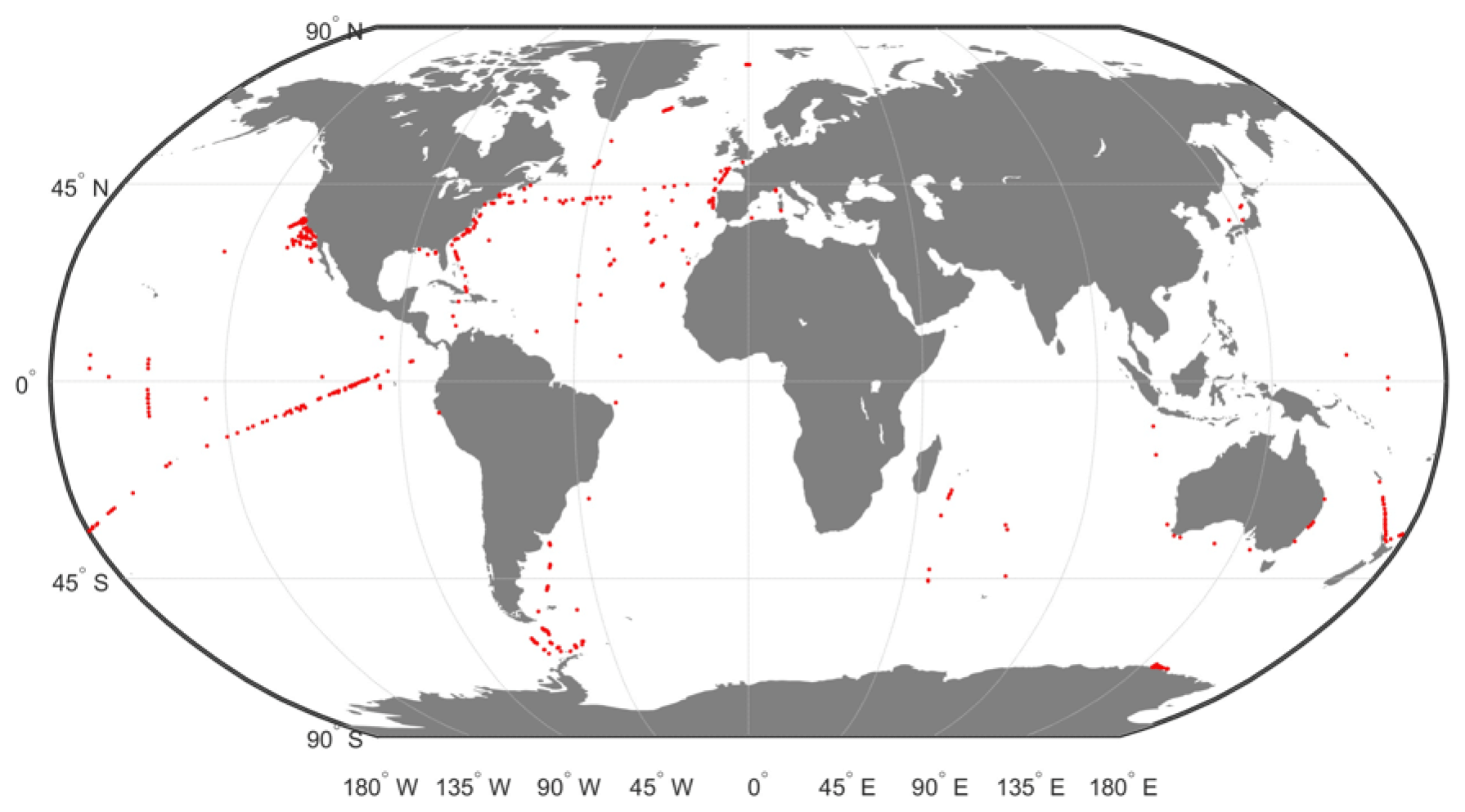
Figure 2 Geographic positions of the 515 in situ and satellite collocated measurements of the DPIG database.

In Fig. 3 we present the R² coefficient between the in situ chl a and the SeaWiFS chl a computed by using the OC4V4 algorithm (O'Reilly et al., 2001) for the DPIG collocated observations. We remark that the two measurements are in good agreement at global scale. Each data point of DPIG is a vector having 17 components (five ocean reflectance ρ_w(λ) and Ra(λ) at five wavelengths (412, 443, 490, 510 and 555 nm), SeaWiFS chl a, five in situ pigment ratios, and in situ chl a concentration). The in situ chl a concentration ranges between 0.007 and 3 mg m⁻³ (see Table 1).

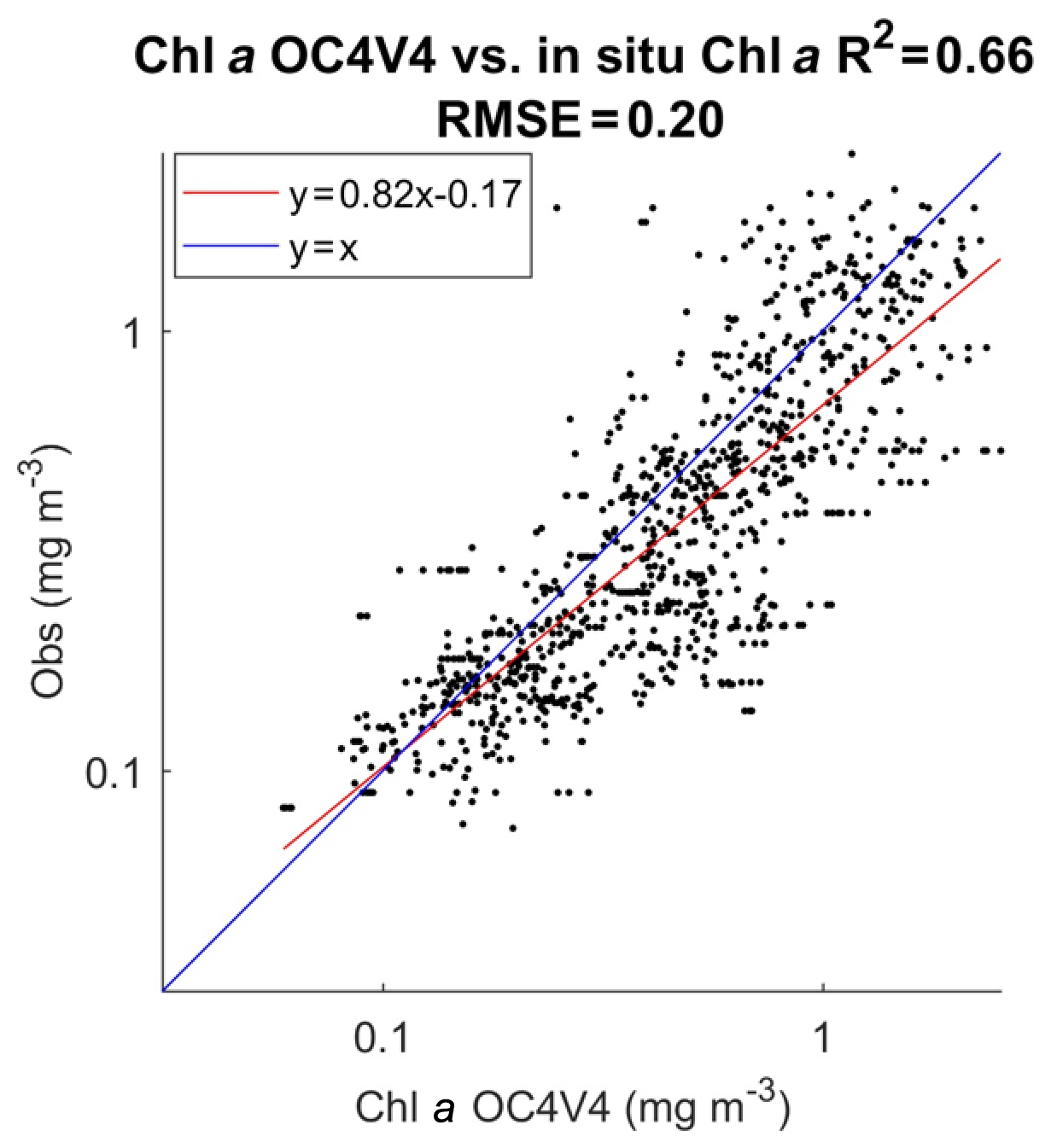
Figure 3 Dispersion diagram of DPIG chl a computed from the SeaWiFS observations using the OC4V4 algorithm versus in situ chl a. The coefficient of determination R² and the RMSE (root mean square error) were computed in milligrams per cubic meter (mg m⁻³).

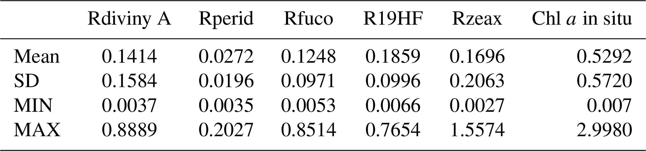
Table 1 Pigments of the DPIG and their statistical characteristics: SD (standard deviation), MIN (minimum value), MAX (maximum value).

The five Ra(λ) are defined following Alvain et al. (2012):

$$\begin{array}{}\text{(2)}& \text{Ra}\left(\mathit{\lambda }\right)={\mathit{\rho }}_{\mathrm{W}}\left(\mathit{\lambda }\right)/{\mathit{\rho }}_{\mathrm{Wref}}(\mathit{\lambda },\mathrm{chl}a),\end{array}$$

where the parameter ρ_Wref(λ,chl a) is an average reflectance depending on the chl a concentration only that was computed according to the procedure reported in Farikou et al. (2015). Ra(λ) is a nondimensional parameter that depends on the chl a abundance at second order and is mainly sensitive to the secondary pigments (Alvain et al., 2012).

The DPIG database thus provides information on the existing links between the pigment composition and the SeaWiFS measurements. The pigment composition is defined by the pigment ratios, which are nondimensional variables of the form in the present study:

$$\begin{array}{}\text{(3)}& \text{pigment ratio}=\text{DP}/\mathrm{Tchl}a,\end{array}$$

which is defined as the ratio of the diagnostic pigment (DP) versus the total chl a (Tchl $a=\mathrm{chl}a+\text{divinyl}\mathrm{chl}a$), according to Alvain et al. (2005).

The pigments of the DPIG and their statistical characteristics are given in Table 1. The statistical tests presented in Fig. 3 (R² and RMSE) and in Table 1 (MEAN, SD, MIN, MAX) were computed in milligrams per cubic meter (mg m⁻³).

2.2 The Senegalo–Mauritanian upwelling satellite data (DSAT)

The satellite dataset we processed to retrieve the pigment concentration consists of five ρ_w(λ) and five Ra(λ) at five wavelengths (412, 443, 490, 510 and 555 nm), as well as the SeaWiFS chl a concentration observed in the Senegalo–Mauritanian upwelling region (8–24^∘ N, 14–20^∘ W; Fig. 3) during 11 years (1998–2009) by SeaWiFS. This dataset is denoted here as DSAT.

The satellite observations (ρ_w(λ) and chl a concentration) were provided by NASA with a resolution of 9 km. Due to the presence of Saharan dust in this region, very few estimations of satellite ρ_w(λ) and in situ chl a were available, and some satellite estimations of chl a could present strong overestimations (Gregg et al., 2004). For this reason, we reprocessed the ρ_w(λ) and chl a data with an atmospheric correction algorithm developed specifically for Saharan dust (Diouf et al., 2013; http://poacc.locean-ipsl.upmc.fr/, last access: 4 March 2020) in order to improve the satellite observations.

2.3 The UPSEN database

Recently, some HPLC measurements were made in the Senegalo–Mauritanian region during two oceanographic cruises (UPSEN campaigns) of the oceanographic ship Le Suroit from 7 to 17 March 2012 and from 5 to 26 February 2013 as reported in Ndoye et al. (2014) and Capet et al. (2017). The goal was to study the dynamics and the biological variability of the Senegalo–Mauritanian upwelling. During these campaigns, in situ HPLC measurements were carried out. We expected to be able to collocate them with the ocean-color VIIRS (Visible Infrared Imaging Radiometer Suite) sensor observations, whose wavelengths are close to those of the SeaWiFS. Unfortunately, we were only able to process satellite observations made on 21 February 2013 due to the presence of clouds and Saharan aerosols the other days. We processed the satellite observations provided by the VIIRS sensor at four wavelengths (443, 490, 510, 555 nm) for pixels in the vicinity of the ship stations (within a distance of 20 km) observed in a time window of ±12 h and for which the satellite chl a was less than 3 mg m⁻³, which is the limit of validity of our method imposed by the range of chl a observed in DPIG (mean of 0.52 mg m⁻³). Only five stations off the Cabo Verde peninsula fit these requirements (see Fig. 1 for their positions).

3 The proposed method (2S-SOM)

Classification methods were applied to retrieve geophysical parameters from large databases in several studies including weather forecasting (Lorenz, 1969; Kruizinga and Murphy, 1983), short-term climate prediction (Van den Dool, 1994), downscaling (Zorita and von Storch, 1999), reconstruction of oceanic pCO₂ (Friedrichs and Oschlies, 2009) and chl a concentration under clouds (Jouini et al., 2013). In the present study, we used a new neural network classifier, which is an extension of the SOM algorithms.

3.1 The SOM clustering

The SOM algorithms (Kohonen, 2001) constitute powerful nonlinear unsupervised classification methods. They are unsupervised neural classifiers that have been commonly used to solve environmental problems (Cavazos, 2000; Hewitson and Crane, 2002; Richardson et al., 2003; Liu and Weisberg, 2005; Liu et al., 2006; Niang et al., 2003, 2006; Reusch et al., 2007). The SOM aims at clustering vectors z_i∈ℝ^N of a multidimensional database D. Clusters are represented by a fixed network of neurons (the SOM), each neuron c being associated with the so-called referent vector w_c representing a cluster. The self-organizing maps are defined as an undirected graph, usually a rectangular grid of size p×q. This graph structure is used to define a discrete distance (denoted by δ) between two neurons of the p×q rectangular grid that presents the shortest path between two neurons. Each vector z_i of D is assigned to the neuron whose referent w_c is the closest in the sense of the Euclidean distance: w_c is called the projection of the vector z_i on the map. A fundamental property of an SOM is the topological ordering provided at the end of the clustering phase: close neurons on the map represent data that are close in the data space. The estimation of the referent vectors w_c of an SOM and the topological order is achieved through a minimization process in which the referent vectors w are estimated from a learning dataset (the DPIG database in the present case). The cost function is shown in Appendix A.

The SOMs have frequently been used in the context of completing missing data (Jouini et al., 2013), so the projected vectors z_i may have missing components. Under these conditions, the distance between a vector z_i∈D and the referent vectors w_c of the map is the Euclidean distance that considers only the existing components (the truncated distance or TD hereinafter).

3.2 The 2S-SOM classifier

In the present case, we used the 2S-SOM algorithm, a modified version of the SOM, which is very powerful in the case of a large number of variables. It automatically structures the variables having some common characteristics into conceptually meaningful and homogeneous blocks. The 2S-SOM takes advantage of this structuration of D and the variables into different blocks, which permits an automatic weighting of the influence of each block and consequently of each variable. The block weighting facilitates the clustering procedure by considering the most pertinent variables. The vectors of DPIG defined in Sect. 2 can be decomposed into four blocks. The essence of this decomposition into blocks is that each of the 17 components of the DPIG vectors gathers information with a different physical influence in the classification phase. The composition of each block is done as follows.

The 2S-SOM is able to deal with a large quantity of variables, choosing those that are the most significant for the classification and neutralizing those that are the least significant. This is done by estimating weights on the blocks and the variables. We fully describe the 2S-SOM algorithm in Appendix A. In the following we use a simplified version of 2S-SOM in which only the blocks are weighted.

3.3 The calibration phase

Similarly to the standard SOM, the 2S-SOM is determined through a learning phase by using a more complex cost function (see Appendix A) that estimates for each neuron, in addition to the referent vector, a weight (α) for each block. For a neuron c, we define the weights of each block b (b=1…4).

At the end of the calibration phase, each element z_i of the dataset DPIG is associated with a referent w_c whose components are partitioned into four blocks. In the present study, the 2S-SOM is represented by a two-dimensional ($\mathrm{9}\times \mathrm{18}=\mathrm{162}$) grid that represents the partition of the DPIG dataset into different classes. Each class provided by the 2S-SOM is associated with a so-called referent vector w_c with c∈{1…162}. The size of the map has been determined by using the procedure provided by the SOM software available at http://www.cis.hut.fi/projects/somtoolbox/download/ (last access: 4 March 2020).

3.4 The pigment retrieval

In the second phase, which is an operating phase, we estimated the pigment concentration ratios of a pixel from its satellite ocean-color sensor observations only. The 11 ocean-color satellite observations (5ρ_w(λ), 5Ra(λ) and chl a) of pixel PX_m were projected onto the 2S-SOM using the truncated Euclidian distance (Sect. 3.1). We select the neuron c associated with a referent vector whose 11 ocean-color parameters are the closest to those observed by the satellite sensor. The pigment ratios PX_m are those associated with the neuron c. At the end of the assignment phase, each pixel PX_m of a satellite image is associated with a referent vector w_c, which has six pigment concentration ratios among its 17 components. The flowcharts of the method (2S-SOM learning and pigment retrieval) are presented in Fig. 4.

Figure 4 Flowchart of the method: (a) learning phase; (b) operational phase that consists of pigment retrieval and the determination of the block parameters.

4 Methodological results

4.1 Statistical validation of the method

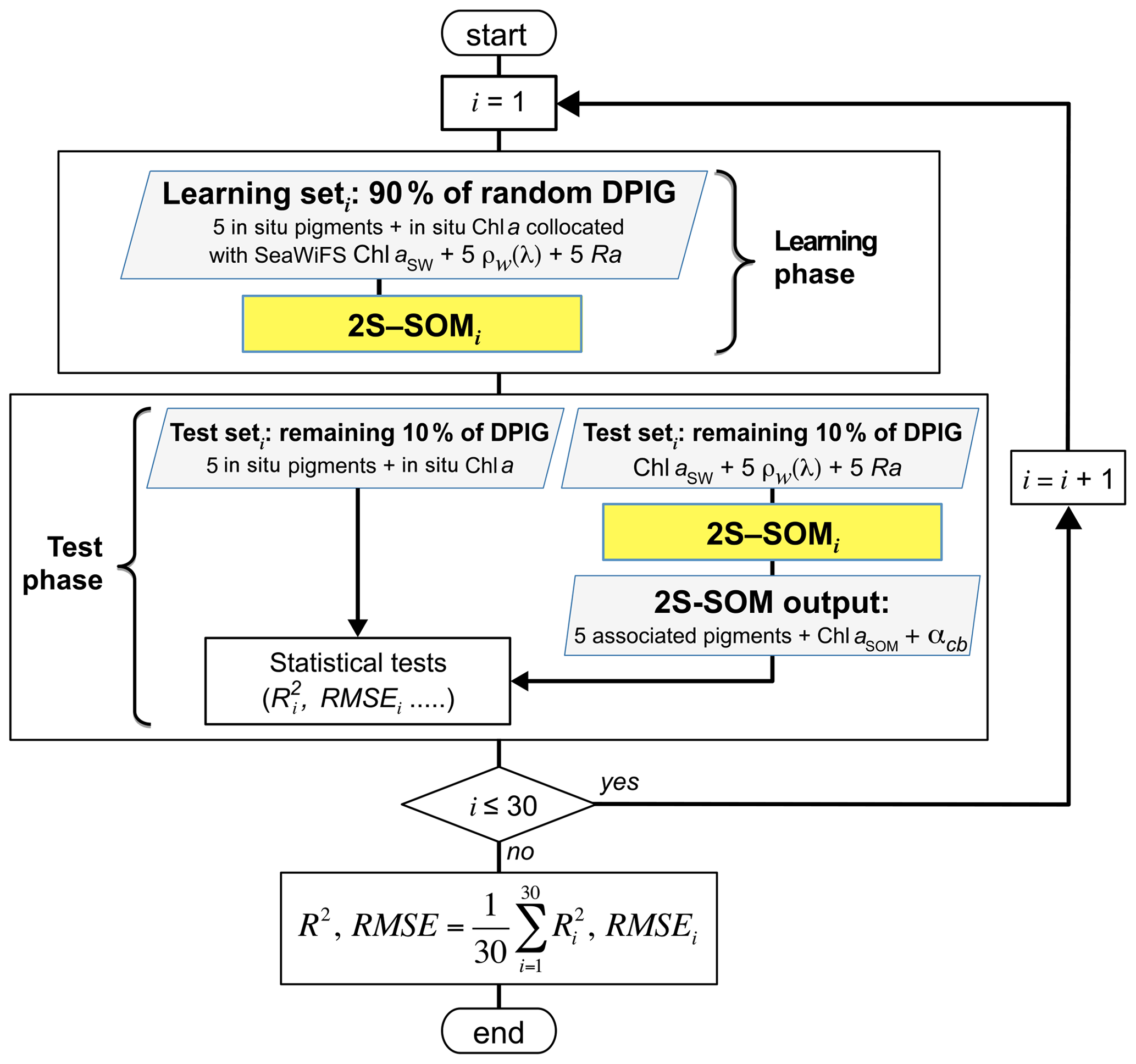
The validation of the method was focused on the retrieval of the fucoxanthin ratio, which is a characteristic of diatoms, but the same procedure could be applied to any pigment. The hyper-parameter μ (see Appendix A) was optimized in order to retrieve that ratio, while η was set as constant since only the blocks were weighted in the present study. Due to the small amount of data in the DPIG, we estimated the accuracy of the fucoxanthin retrieval by a cross-validation procedure, which is a powerful procedure in statistics. The principle is the following: we learned 30 2S-SOMs using 30 different learning datasets L_i constituting 90 % of DPIG taken at random, and then we computed a statistical estimator on the retrieved quantities using 30 test datasets (10 % of DPIG). The algorithm was as follows.

•  

  Starting with i=1…30:

  • 1.

    determination at random of a learning dataset L_i (90 % of DPIG) and a test dataset TL_i (10 % of DPIG);

  • 2.

    training of a 2S-SOM M_i using L_i (see Sect. 3.2 and 3.3);

  • 3.

    validation using TL_i according to the procedure described in Sect. 3.4; and

  • 4.

    estimation of the RMSE_i and $R_i^{\mathrm{2}}$ on TL_i between the estimated and observed fucoxanthin ratios.

The flowchart of the cross-validation procedure is presented in Fig. 5 for the computation of the mean RMSE and R² (R², $\text{RMSE}=\frac{\mathrm{1}}{\mathrm{30}}{\sum }_{i=\mathrm{1}}^{I=\mathrm{30}}{R}^{\mathrm{2}}i,\text{RMSE}i)$.

Figure 5 Flowchart of the cross-validation procedure for 30 partitions of the DPIG database.

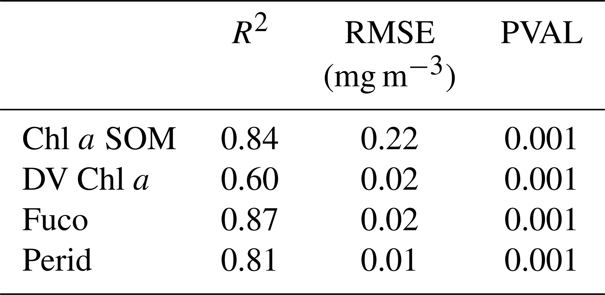
Statistical parameters (R² coefficients, RMSE and P values) of the cross-validation between the DPIG in situ pigments and the pigments given by the 2S-SOM averaged for the 30 2S-SOM realizations, which are presented in Table 2, show the good performance of the method.

Table 2 Statistical parameters (R² coefficients, RMSE and P values) of the cross-validation between the DPIG in situ pigments and the pigments given by the 2S-SOM averaged for the 30 2S-SOM realizations.

4.2 Analysis of the topology of the 2S-SOM

As explained in Sect. 3.2 and 3.3, the referent vector components (w_c∈R¹⁷), which are estimated during the learning phase, are partitioned into four blocks B1, B2, B3 and B4. The hyper-parameter μ was tuned in order to favor the accuracy of the retrieval of the fucoxanthin ratio. We recall that all the pigment ratios are estimated during the calibration phase, but in the present paper attention was focused on the fucoxanthin ratio when selecting the parameter μ. In Fig. 6, we present six of the referent vector components of the 2S-SOM. These components are ρ_w(490), Ra(490), SeaWiFS chl a, and the ratios of fucoxanthin, which is a specific diatom pigment, and of peridinin and divinyl. They exhibit a coherent topological order, with the components having values that are close together on the topological map. The remaining 11 components (not shown) exhibit the same coherent topological order. One can observe a very good topological order for the fucoxanthin ratio that was favored by the determination of the hyper-parameter μ. Moreover, the bottom right region in the 2S-SOM (Fig. 6) may correspond to the diatoms with a good confidence since high fucoxanthin is associated with a high chlorophyll concentration and low peridinin. This is confirmed in Sect. 5 by looking at the geographical location of the different pigment concentrations (Figs. 8, 10, 11). Another important remark is that the value of each component presents a large range of variation of the same order as the range of variation found in the DPIG variables. This means that the 2S-SOM has captured most of the variability of the dataset.

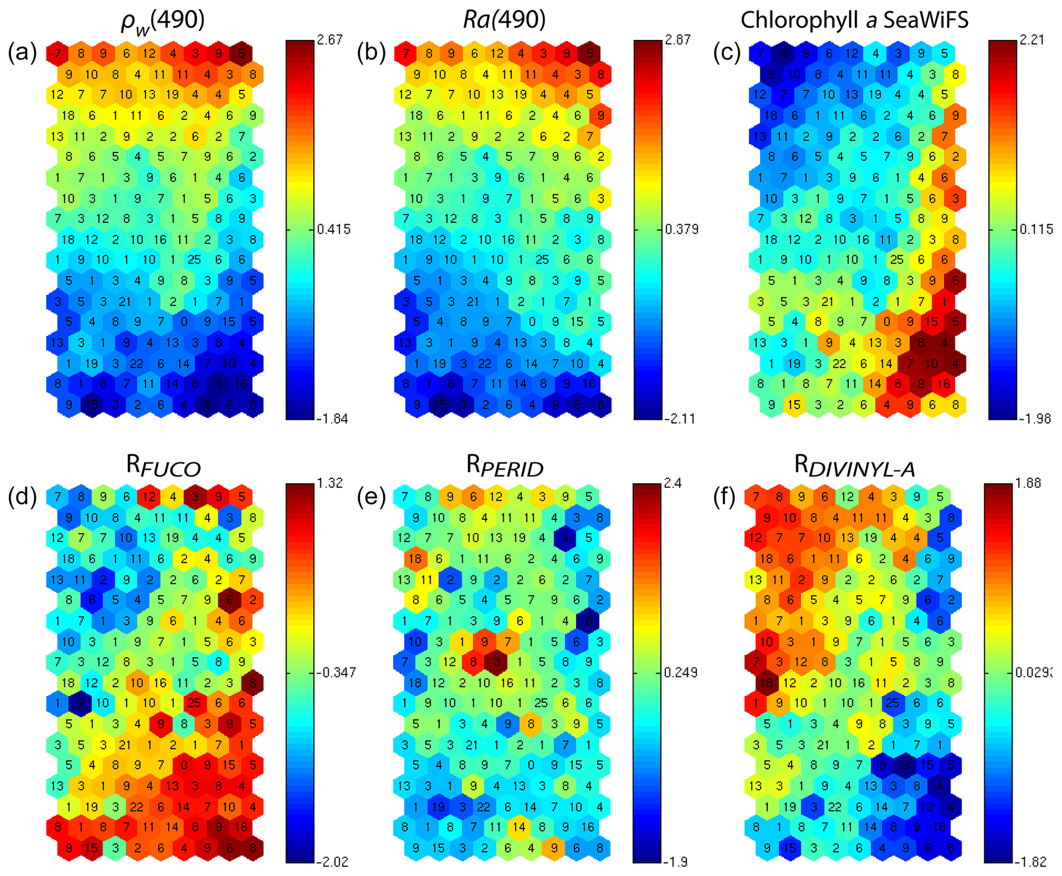
Figure 6 2S-SOM. From left to right and top to bottom, values of the referent vectors for (a) ρ_w(490), (b) Ra(490), (c) SeaWiFS chl a, and the (d) fucoxanthin, (e) peridinin and (f) divinyl ratios. The number in each neuron indicates the amount of DPIG data captured at the end of the learning phase; the values indicated by the color bars are centered–reduced nondimensional values.

Figure 6 shows a strong link between the values of the referent vectors for fucoxanthin and chl a (high fucoxanthin and chl a values at the bottom right of the 2S-SOM), while fucoxanthin is high and chl a low for the referent vectors at the bottom left of the 2S-SOM. Additional information will be provided by the Ra(490) values when the fucoxanthin is less closely linked to the chlorophyll.

In addition, for each neuron, the 2S-SOM provides a weight for each block (α_cb) and each variable (β_cbj). For a given neuron c the weights (α_cb) of the blocks are normalized, their sum being 1. A value of 1 for one block (and therefore a value of 0 for the other blocks) indicates that the data in the neuron are gathered with respect to that block only because there is too much noise in the variables in the other blocks. By examining the weights on the map, one can see which block most influences the link between the satellite measurements and the pigment ratios.

In Fig. 7, we present the α_cb values estimated during the learning phase of the four blocks (B1, B2, B3, B4). For some neurons, only the blocks related to the reflectance and the reflectance ratio are used for the definition of the neuron, while the weights for the two other blocks (pigments and chl a) are null, indicating that for these neurons, in situ observations and SeaWiFS chl a are more noisy than the reflectance. These neurons correspond to very small chl a concentrations, which are estimated with large error. We remark that high α values for chl a correspond to high chl a concentration values (bottom right of the chl a panel in Figs. 7 and 6). For these cases, the clustering assembled data that mainly depend on chl a concentration.

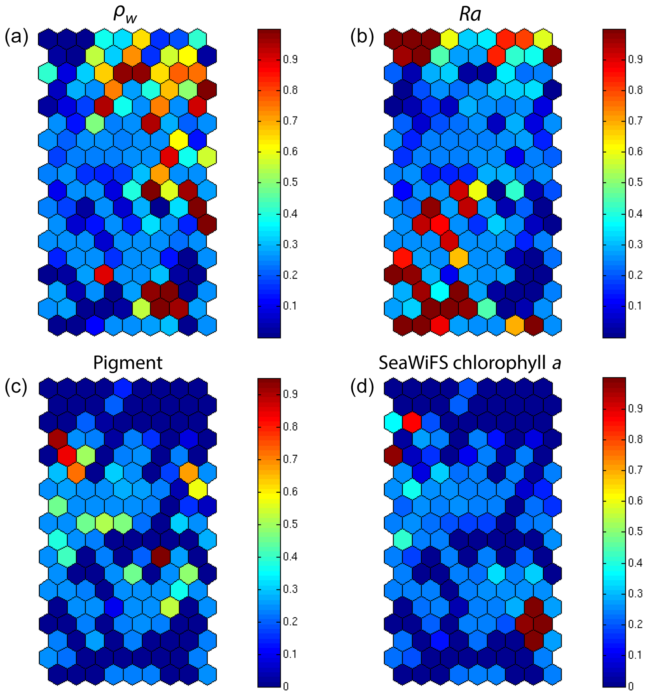
Figure 7 2S-SOM. Weights (α_cb) of the four block parameters determined at the end of the learning phase; (a) ρ_w, (b) Ra, (c) pigment, (d) SeaWiFS chl a. The color bars show the percent of the weight estimated by 2S-SOM, with a value of 1 or 0 indicating that the data in the neuron are assembled with respect to that block only.

5 Geophysical results

In the present study, we apply the 2S-SOM (Sect. 3), which explicitly makes weighted use of the data according to their specificity (ocean-color signals or in situ observations) to retrieve the fucoxanthin concentration from remotely sensed data in the Senegalo–Mauritanian upwelling region where in situ measurements are lacking. According to the good results of the cross-validation method as shown in Sect. 4.1, we expect that the 2S-SOM will provide pertinent results in a region that has been poorly surveyed.

5.1 The pigment estimation from SeaWiFS observations in the Senegalo–Mauritanian upwelling region

We decoded the DSAT database (Sect. 2.3) using the 2S-SOM for 11 years (1998–2009) of SeaWiFS data observed in the Senegalo–Mauritanian upwelling region (8–24^∘ N, 14–20^∘ W). This study was done according to the retrieval phase described in Sect. 3.4. For each day, we projected the 11 SeaWiFS observations (5ρ_w(λ), 5Ra(λ) and chl a) of each pixel on the 2S-SOM. At the end of the assignment phase, each pixel of a satellite image was associated with six pigment concentration ratios. The underlying assumption is that the link between the remote sensing information and the pigment ratios of a pixel is provided by the selected referent w_c. Thanks to the topological order provided by the 2S-SOM, we expected that the best neurons chosen during the retrieval would give accurate concentration ratios. In Figs. 8, 10 and 11 we present the fucoxanthin concentration ratio estimation for 3 different days and the associated SeaWiFS chlorophyll images (1 and 6 January and 28 February 2003). Due to the limited size of the DPIG, the range of the ratio learned for fucoxanthin is between 0.3 % and 20 % with a mean of 10 %, and the chl a content is between 0.5 and 3 mg m⁻³. The statistical estimator we used cannot extrapolate what has not been learned, and for that reason we flagged the pixels in the SeaWiFS images that have a chl a concentration greater than 3 mg m⁻³.

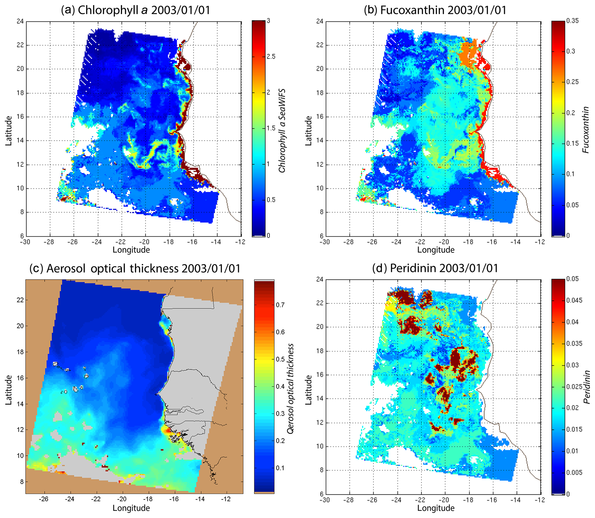
Figure 8 (a) Chl a concentration, (b) fucoxanthin ratio and (c) aerosol optical thickness, (d) peridinin for 1 January 2003. Panels (b, d) show that second-order information was retrieved, which is correlated with the chl a concentration (a) but not equivalent. The aerosol optical thickness (c) does not seem to contaminate the estimated parameters (fucoxanthin and peridinin ratios).

Regarding the images obtained for 1 January 2003 in the Senegalo–Mauritanian region (Fig. 8a–d), we observe that the chl a (Fig. 8a) is very high at the coast and decreases offshore in accordance with the upwelling intensity as shown in the sea surface temperature (SST) image (Fig. 9). Moreover, we observed a persistent well-marked chl a pattern south of the Cabo Verde peninsula in the form of a W, which is the signature of a baroclinic Rossby wave (Sirven et al., 2019).

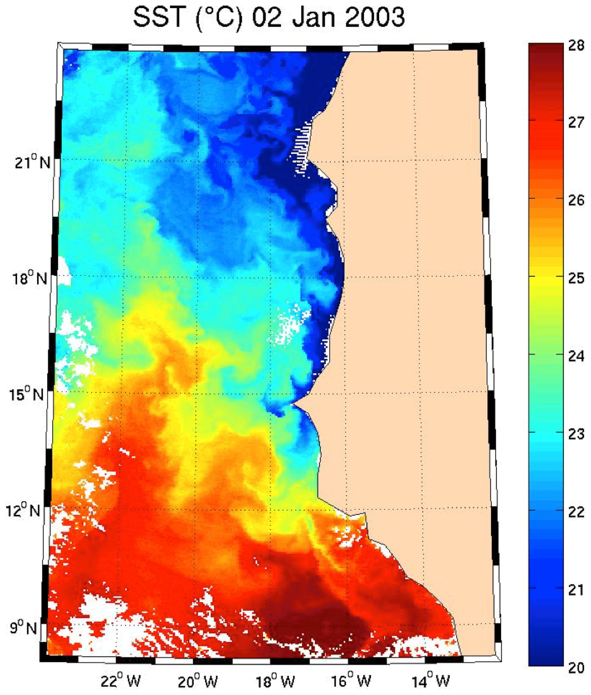
Figure 9 SST for 2 January 2003. Note the well-marked upwelling (cold temperature) north of 13^∘ N.

Except in the southern part of the region, the AOT (aerosol optical thickness) is low; this means that the atmospheric correction of the reflectance is quite small, which gives confidence in the ocean-color data products. The fucoxanthin concentration is maximum at the coast and decreases offshore as does the chl a concentration, in agreement with the works of Uitz et al. (2006, 2010). Fucoxanthin presents coherent spatial patterns. The peridinin concentration is somewhat complementary to that of fucoxanthin, with the low fucoxanthin concentration area corresponding to the high peridinin concentration area (northern part of Fig. 8b, d). This behavior is also observed in Fig. 10 (6 January 2003) and in Fig. 11 (28 February 2003), supporting the analysis shown in Fig. 8.

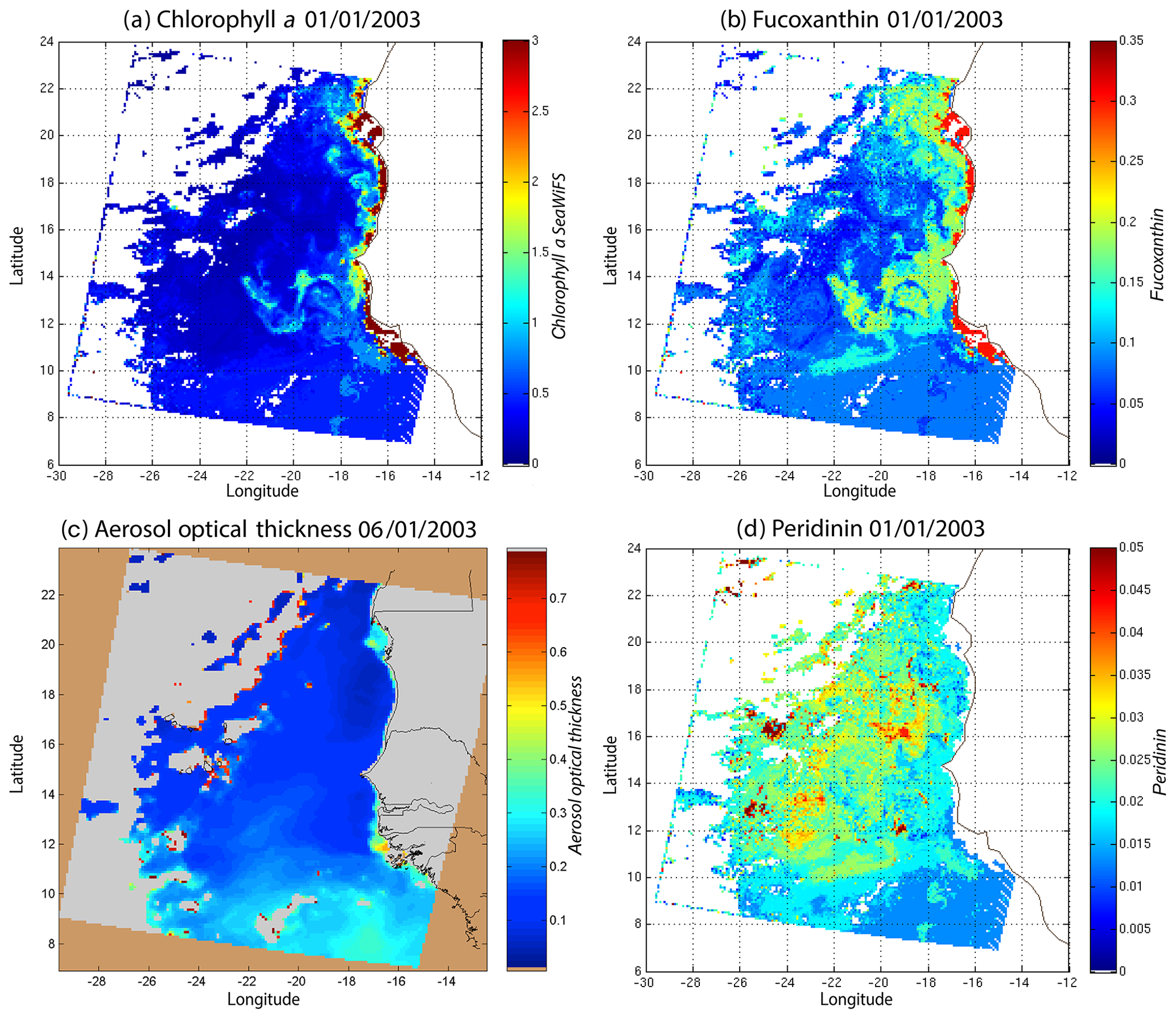
Figure 10 (a) Chl a concentration, (b) fucoxanthin ratio, (c) aerosol optical thickness and (d) peridinin for 6 January 2003. Panels (b, d) show that second-order information was retrieved, which is correlated with the chl a concentration (a) but is not equivalent. It is found that the aerosol optical thickness (c) does not contaminate the estimated parameters (fucoxanthin and peridinin ratios).

Figure 11 (a) Chl a concentration, (b) fucoxanthin ratio, (c)  aerosol optical thickness and (d) peridinin for 28 February 2003. Panels (b, d) show that second-order information was retrieved, which is correlated with the chl a concentration (a) but is not equivalent. It is found that the aerosol optical thickness (c) does not contaminate the estimated parameters (fucoxanthin and peridinin ratios). The positions of the NSB and OFB are outlined by black square boxes.

For 28 February, we selected two square box regions (Fig. 11), one near the coast (NSB, long. [$-\mathrm{20}{}^{\circ }$, $-\mathrm{18}{}^{\circ }$], lat. [12^∘, 14^∘]) and the other about 800 km offshore (OFB, long. [$-\mathrm{28}{}^{\circ }$, $-\mathrm{26}{}^{\circ }$], lat. [12^∘, 14^∘]). NSB waters correspond to upwelling waters, while OFB waters correspond to oligotrophic waters. We projected the 11 ocean-color parameters of the NSB and OFB pixels on the 2S-SOM.

Figure 12 presents the reflectance spectra (in blue) captured by three neurons of the 2S-SOM corresponding to pixels located in the NSB region (panels a–c) and those captured by three neurons corresponding to pixels located in the OFB region (panels d–f). The reflectance spectra of the associated referent vectors w are in yellow. The satellite reflectance spectra match the referent vector spectra; moreover, the fucoxanthin ratio varies inversely with the mean value of the spectrum: the higher the fucoxanthin ratio, the smaller the mean value of the spectrum. The pigment concentration is greater near the coast.

Figure 12 Reflectance spectra (in blue) captured on 28 February by six neurons whose referent vector spectra are in yellow: (a–c) pixels in the NSB region (long. [$-\mathrm{20}{}^{\circ }$, $-\mathrm{18}{}^{\circ }$], lat. [12^∘, 14^∘]); (d–f) pixels in the OFB region (long. [$-\mathrm{28}{}^{\circ }$, $-\mathrm{26}{}^{\circ }$], lat. [12^∘, 14^∘]).

We note a strong difference between the shape and the intensity of the nearshore (NSB) and offshore (OFB) spectra. The OFB spectra present mean values higher than those of the NSB spectra. This is due to the fact that NSB spectra were observed in a region where diatoms are abundant, as shown by the high value of the fucoxanthin concentration in this region (Figs. 8, 10 and 11), which is a proxy for diatoms along with a higher chl a concentration. In Fig. 12, we note the lower values of the coastal spectra at 443 nm, which can be interpreted as a predominant effect of spectral absorption by phytoplankton pigments and CDOM. The different spectra are close together in the OFB region and more disperse in the NSB region. This can be explained by the fact that the OFB region corresponds to case 1 waters, while the NSB region waters are close to case 2 waters and are influenced by the variability of nearshore process like turbidity or the presence of dissolved matter and dynamical instabilities.

We analyzed the weights of the blocks for the neurons selected in the analysis of the coastal (NSB) and offshore (OFB) boxes. Figure 13 presents the box plot of the weight α_cb corresponding to the neurons belonging to the four blocks (B1, B2, B3, B4), with the constraint that the sum of the weights of a neuron is 1; a weight α larger than 0.25 indicates the predominance of a block in the learning for the classification (see Sect. 3.5). It is clear that the weights for pixels near the coast (Fig. 13a) are different from those for offshore pixels (Fig. 13b). As already mentioned in Sect. 4.3 and also shown in Fig. 7, the weights of the 2S-SOM play a significant role in the 2S-SOM topology and consequently in the pigment retrieval. The weights of blocks B1 and B4 that take into account the influence of the pigment ratios and the chlorophyll content in the retrieval are very low for the offshore (OFB) oligotrophic region and more important for the coastal (NSB) region. The weights of the blocks B2 and B3, which take into account the influence of the reflectance (ρ_w(λ), Ra(λ)), dominate for the offshore regions. In coastal waters, the weights of all the blocks are used, with a smaller influence of B3, which is associated with Ra. This gives information on the role played by the different variables in the classification in waters having different phytoplankton concentrations and compositions. It also shows the automatic adaptation of the 2S-SOM to the environment in order to optimize the clustering efficiency with respect to a classical SOM.

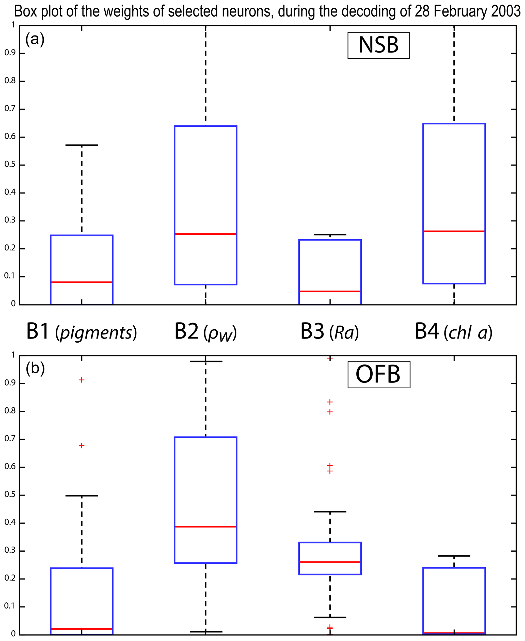
Figure 13 Box plot of the weights of the selected neurons during the decoding of the 28 February data. From left to right are the weights of blocks B1, B2, B3 and B4 (a) n the NSB region (long. [$-\mathrm{20}{}^{\circ }$, $-\mathrm{18}{}^{\circ }$], lat. [12^∘, 14^∘]) and (b) in the OFB region (long. [$-\mathrm{28}{}^{\circ }$, $-\mathrm{26}{}^{\circ }$], lat. [12^∘, 14^∘]).

In order to study the seasonal variability of the fucoxanthin concentration with some statistical confidence in the Senegalo–Mauritanian upwelling region, we constructed a monthly climatology for an 11-year period (1998–2009) of the SeaWiFS observations by summing the daily pixels of the month under study. The resulting climatology is presented in Fig. 14 for December (Fig. 14a), March (Fig. 14b) and May (Fig. 14c), which correspond to the most productive period (Fig. 14c). The fucoxanthin concentration, and consequently the associated diatoms, presents a well-marked seasonality. Fucoxanthin starts to develop in December north of 19^∘ N, presents its maximum intensity in March when the upwelling intensity is maximum, extends up to the coast of Guinea (12^∘ N) in April and begins to decrease in May when it is observed north of the Cabo Verde peninsula (15^∘ N) in agreement with the observations reported by Farikou et al. (2015) and Demarcq and Faure (2000).

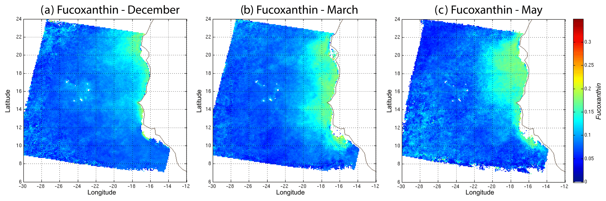
Figure 14 Monthly fucoxanthin concentration averaged over 11 years (1998–2009) for December (a), March (b) and May (c).

Figure 15 shows the fucoxanthin (in green) and the chl a (in blue) concentrations computed from satellite observations for an 11-year period of SeaWiFS observations in the NSB region. There is a good correlation in phase between these two variables but not in amplitude (a good coincidence of peak occurrence but weak correlation in peak amplitude), showing that the relationship between fucoxanthin and chl a is complex as mentioned by Uitz et al. (2006). In particular, there is a weak peak in fucoxanthin in October 2001, which is not correlated with a chl a peak.

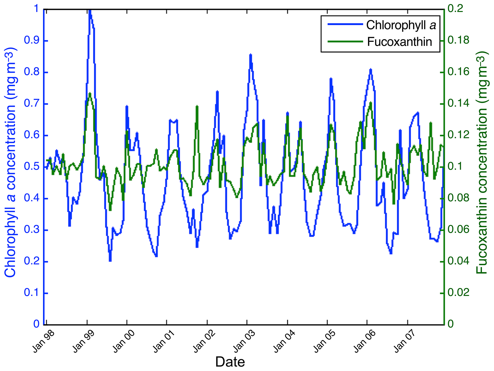
Figure 15 Chl a (in blue) and fucoxanthin (in green) concentrations for nearshore pixels (in the NSB region).

5.2 Analysis of the UPSEN campaigns

Figure 16 shows, for each UPSEN station 1, 2, 3, 5a and 5b (see Fig. 1 for their geographical position), the averaged in situ UPSEN spectrum (in blue) and the referent spectrum (in red) of the 2S-SOM neuron captured by the collocated satellite VIIRS sensor observations. The referent spectrum is the mean of the different spectra captured by that neuron during the learning phase. Among these different spectra, there is one (black curve in Fig. 16) that is the closest to the UPSEN spectrum. Obviously, the black curve is closer to the blue curve than the red one that is flattened due to the averaging process. These three spectra are close together, showing the good functioning of the 2S-SOM.

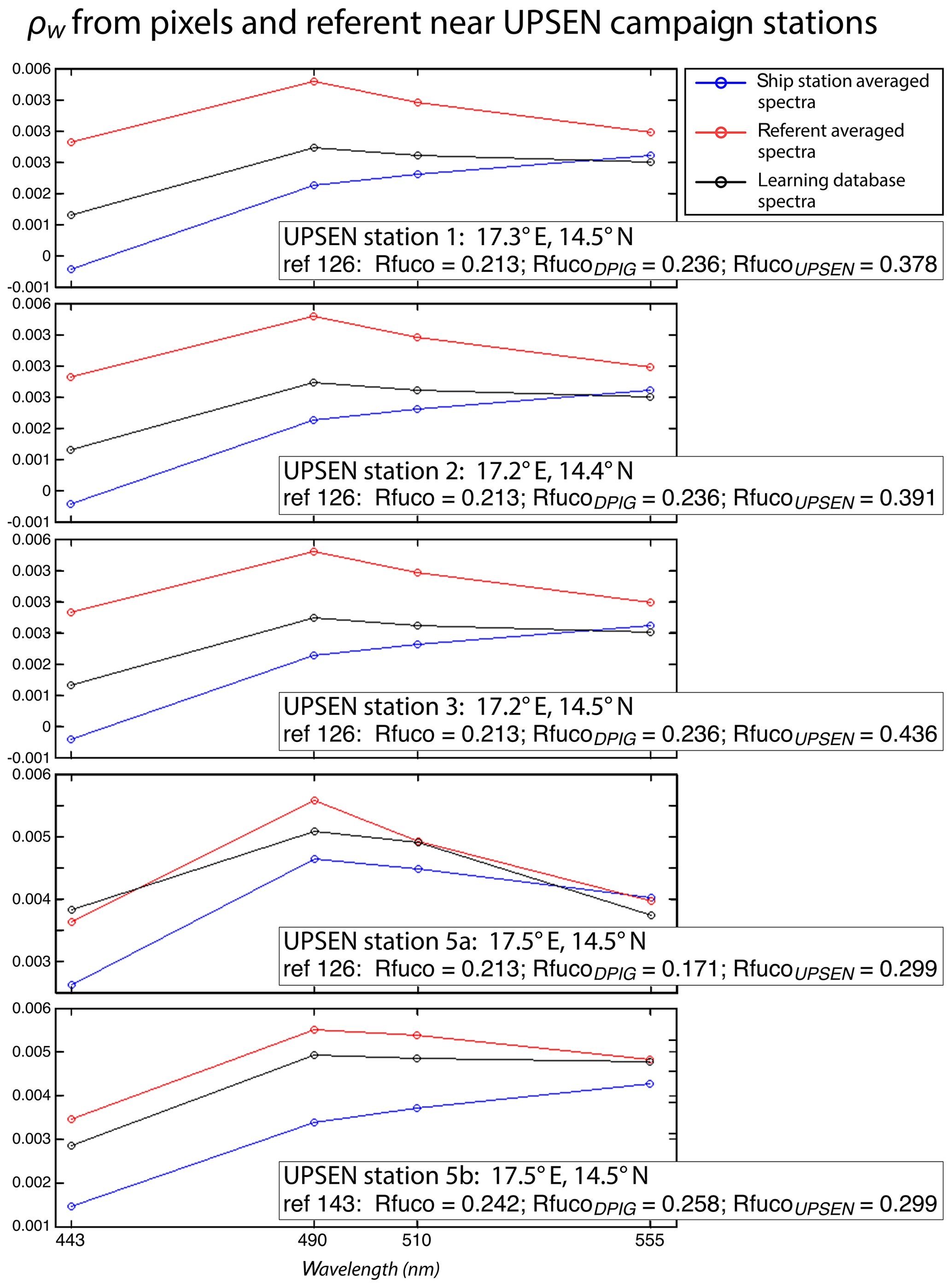
Figure 16 For ship stations 1, 2, 3, 5a and 5b, we show the averaged spectrum of the in situ spectra of the UPSEN stations in blue and the spectrum of the referent vector (in red) of the 2S-SOM neuron that has captured the closest satellite observations to the UPSEN station. Among the different spectra constituting the referent spectrum, the spectrum of the learning database (DPIG) that is the closest to the averaged satellite spectra is shown in black. In the rectangular boxes, we show the position of the UPSEN station, the number of the neuron of the 2S-SOM that has captured the satellite observation, the Rfuco of the referent vector, the Rfuco_DPIG of the closest DPIG and the in situ Rfuco_UPSEN.

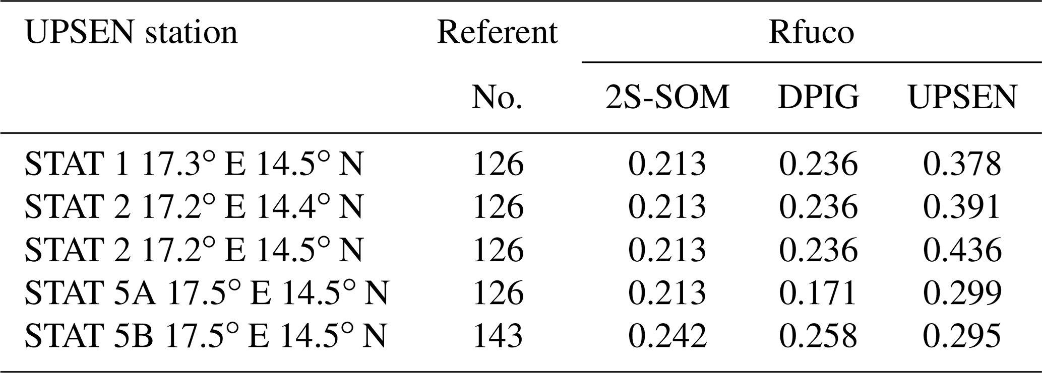
Their shapes are close to those observed in the NSB region (Fig. 12) but their intensity is lower, meaning that their waters are more absorbing than the NSB waters due to a higher pigment concentration. In fact, the UPSEN stations were located close to the coast (Fig. 1) in the Hann bight south of the Cabo Verde peninsula, which is very rich in phytoplankton pigments. In Table 3, we present the fucoxanthin ratios associated with the referent vectors (Rfuco_2S-SOM), the closest DPIG fucoxanthin ratios captured by the neuron of the referents and the fucoxanthin ratios measured during the UPSEN campaign. We note that the fucoxanthin ratios of the in situ measurements are in the range of the DPIG (see Table 1), which allows for the good functioning of the 2S-SOM estimator. The pigment ratios obtained from ocean-color observations through the 2S-SOM are close to pigment concentrations measured at the ship stations, which confirms the validity of the method we have developed. We remark that the best 2S-SOM estimate of the fucoxanthin ratio with respect to the UPSEN in situ measurement is given at station 5b, which is the farthest off the coast. These results support the climatological study of the Senegalo–Mauritanian upwelling region we have done with the 2S-SOM (Sect. 5.1).

Table 3 For ship stations 1, 2, 3, 5a and 5b of the UPSEN campaign, we show the referent captured by the VIIRS observations, the fucoxanthin ratio associated with this referent (Rfuco-2S-SOM), the fucoxanthin ratio of the closest DPIG fucoxanthin ratio captured by the neuron of the referent and the fucoxanthin ratio measured in situ during the UPSEN campaign.

The 2S-SOM method gives pigment concentrations that are close to those obtained by in situ observations. The method could be applied to a large variety of other parameters in the context of studying and managing the planet Earth. The major constraint to obtaining accurate results is to deal with a learning dataset that statistically reflects all the situations encountered in the observations processed. Due to its construction, the method cannot be used to find values beyond the range of the learning dataset.

6 Discussion

Machine-learning methods are powerful methods to invert satellite signals as soon as we have an adequate database to support the calibration. Several techniques have been used for retrieving biological information from ocean-color satellite observations. First, studies have employed multilayer perceptrons (MLPs), which are a class of neural networks suitable to model transfer function (Thiria et al., 1993). Gross et al. (2000, 2004) retrieved the chl a concentration from SeaWiFS, Bricaud et al. (2006) modeled the absorption spectrum with MLP, and Raitsos et al. (2008) and Palacz et al. (2013) introduced additional environmental variables in their MLPs such as SST in the retrieval of PSC and PFT from SeaWiFS, which improved the skill of the inversion. Another suitable procedure was to embed NN in a variational inversion, which is a very efficient way when a direct model exists (Jamet et al., 2005; Brajard et al., 2006a, b; Badran et al., 2008). Statistical analysis of the absorption spectra of phytoplankton and pigment concentrations was conducted by Chazottes et al. (2006, 2007) using an SOM.

In the present study, due to the fact that the learning dataset was quite small (515 elements), we used an unsupervised neural network classification method, which is an extension of the SOM method well adapted to dealing with a small database whose elements are very inhomogeneous. We clustered available satellite ocean-color reflectance at five wavelengths and their derived products, such as chlorophyll concentration and the associated in situ pigment ratios.

The major points of this study are as follows.

• 1.

  The clustering was carried out by developing a new neural classifier, the so-called 2S-SOM, which presents several advantages with respect to the classical SOM. As in the SOM, we defined clusters that assemble vectors that are close together in terms of a specified distance. This classifier was learned from a worldwide database (DPIG) whose vectors are ocean-color parameters observed by satellite multispectral sensors and associated pigment concentrations measured in situ. In the operational phase, SeaWiFS images are decoded, allowing for the estimation of the pigment concentration ratios. The major advantage of 2S-SOM with respect to the classical SOM is to cluster variables having similar physical significance into blocks having specific weights. The weights attributed to the four blocks are computed during the learning phase and vary with the quality of the variables and with respect to their location in the ocean (near the coast or offshore). This permits us to modulate the variable influence in the cost function, which makes the clustering more informative than that provided by the SOM. The block decomposition provides useful scientific information. For offshore, the weight analysis allowed us to show that more influence is given to the reflectance ratios Ra(λ) and less to the chl a and pigment concentrations; in contrast, near the coast the weights indicate a more active use of the pigment composition and the chl a concentration. Therefore, the resulting 2S-SOM clustering at best takes into account the information that belongs to the specific water content.

• 2.

  The 2S-SOM decomposes the DPIG into a large number of significant ocean-color classes, allowing for the reproduction of the different possible situations encountered in the dataset we analyze. We assume that the relationship between the pigment concentration and the remotely sensed ocean-color observations is independent of the location, which is justifiable since the relationship depends on the optical properties of ocean waters through well-defined physical laws that are region-independent. This also supports the fact that we used a global database to retrieve pigments in a definite region. In contrast, the different phytoplankton species vary from one region to another, making the relationship between the pigment ratio and phytoplankton species strongly dependent on the region. This justifies the fact we focused our study on the pigment retrieval rather than on the PSC or PFT, as mentioned above. Moreover, most of the recent phytoplankton in situ identifications have been made using pigment measurements with the HPLC method (Hirata et al., 2011). It is therefore more natural to retrieve the pigment concentration, which is the quantity we measured, than the associated PSC or PFT, which are estimated from the pigment observations through complex nonlinear and region-dependent algorithms (Uitz et al., 2006). Due to the characteristics of the DPIG, the method can retrieve pigment concentration patterns over a large range (0.02–2 mg m⁻³).

• 3.

  We were able to analyze the pigment concentration in the Senegalo–Mauritanian region by processing satellite ocean-color observations with the 2S-SOM. We found an important seasonal signal of fucoxanthin concentration with a maximum occurring in March. We found evidence of a large offshore gradient of fucoxanthin concentrations, the nearshore waters being richer than the offshore ones. We showed that the offshore region waters correspond to case 1 waters, while the nearshore waters are close to case 2 waters and are influenced by the variability of nearshore process like turbidity or the presence of dissolved matter. The UPSEN measurements show that the pigment ratios of the Senegalo–Mauritanian region are in the range of the DPIG database used to calibrate the method, which justifies the use of the 2S-SOM algorithm to investigate this region.

• 4.

  We used daily satellite observations to construct a monthly climatology of pigment concentrations of the Senegalo–Mauritanian upwelling region, which has been poorly surveyed by oceanic cruises. Due to the highly nonlinear character of the algorithms for determining the pigment concentrations from satellite measurements, it is mathematically more rigorous to apply these algorithms to daily satellite data and average this daily estimate for the climatology period under study than to estimate them from the satellite data climatology, as many authors have done (Uitz et al., 2010; Hirata et al., 2011). We found that fucoxanthin starts developing in December north of 19^∘ N, presents its maximum intensity in March when the upwelling intensity is maximum, extends up to the coast of Guinea (12^∘ N) in April and begins to decrease in May.

Another important aspect of our study concerns the validity of our results. The 2S-SOM method has been validated by focusing the retrieval accuracy on the fucoxanthin ratio by using a cross-validation procedure. These results were qualitatively confirmed by two other independent studies.

• -

  We first applied a cross-validation procedure (see Sect. 4.1), which is a powerful technique for validating models (Kohavi, 1995; Varma and Simon, 2006). We learned 30 different 2S-SOMs using 30 different learning dataset determined at random from the DPIG dataset (each learning dataset representing 90 % of DPIG) and 30 test datasets (10 % of DPIG). By averaging the results, we found that the 2S-SOM method retrieves the fucoxanthin concentration with a good score (see the statistical parameters in Table 2), which confirms the pertinence of the method.

• -

  We then found that our fucoxanthin climatology is in agreement with in situ observations of phytoplankton reported in Blasco et al. (1980) in March to May 1974 off the coast of Senegal during the JOINT I experiment. These authors analyzed 740 water samples collected with Niskin bottles at 136 stations extending along a line at 21^∘40^′ N (in the northern part of the studied region) from 0 to 100 km offshore. The samples were taken at several depths (mostly at 100, 50, 30, 15, 5 m). Phytoplankton cells were counted and identified by the Utermöhl inverted microscope technique (Blasco, 1977). These authors found that diatoms reach their maximum concentration in April–May and are the most abundant group in that period, whereas the other cells predominate in March. Similar microscope observations were reported in the ocean area south of Dakar by Dia (1985) during several ship surveys in February–March 1982–1983.

• -

  Our method is also in agreement with the monthly 11-year climatology presented in Farikou et al. (2015), who used a modified PHYSAT method to retrieve the PFT in the Senegalo–Mauritanian region.

• -

  The pigment concentrations provided by the 2S-SOM from the VIIRS sensor observations are in qualitative agreement with the in situ measurements done at five stations during the two UPSEN campaigns in 2012 and 2013, showing that the method is able to function in waters where the pigment concentrations are quite high (fucoxanthin ratios of the order of 0.4).

7 Conclusions

We developed a new neural network clustering method, the so-called 2S-SOM algorithm, to retrieve phytoplankton pigment concentration from satellite ocean-color multispectral sensors. The 2S-SOM algorithm is an SOM specifically designed to deal with a large number of heterogeneous components such as optical and chemical measurements. The major advantage of 2S-SOM with respect to the classical SOM is to cluster variables having similar significance into blocks having specific weights. The weights attributed to the blocks during the learning phase vary with the quality of the variables in the classification. This permits us to modulate the variable influence in the cost function, which makes the clustering more informative than that provided by the SOM. The block weighting provides useful information on the functioning of the classification by permitting us to identify the variables that control it. It also allows us to better understand the dynamics of the phytoplankton communities.

The 2S-SOM method is efficient and rapid as soon as the calibration is done, since it uses elementary algebraic operations only. The 2S-SOM method is like a piecewise regression that takes advantage of the unsupervised classification of the SOM. We decomposed the DPIG database into quite a large number of partitions ($\mathrm{9}\times \mathrm{8}=\mathrm{162}$) when comparing our study to other studies (Uitz et al., 2006). The validity of the method has been controlled through a cross-validation procedure and confirmed by three qualitative studies. Statistical parameters (R² coefficients, RMSE and P values) of the cross-validation between the DPIG in situ pigments and the pigments given by the 2S-SOM averaged for the 30 2S-SOM realizations presented in Table 2 show the good performance of the method. It must be noted that the performance mainly depends on the size of the learning set used to calibrate the 2S-SOM. This set must include all the situations encountered in the pigment retrieval. The larger the learning set, the better the method performs. Due to its generic character and its flexibility, the method could be used to determine a large variety of measures with satellite remote sensing observations.

In this work, the method was applied to study the seasonal variability of the fucoxanthin concentration in the Senegalo–Mauritanian upwelling region. We showed a large offshore gradient of fucoxanthin, the higher concentration being situated near the shore. We were able to construct a monthly climatology for an 11-year period (1998–2009) of the SeaWiFS observations by summing the daily pixels of the month under study in a region that was poorly surveyed by oceanic cruises. The fucoxanthin concentration, and consequently the associated diatoms, presents a well-marked seasonality (Fig. 10). Fucoxanthin starts developing in December north of 19^∘ N, presents its maximum intensity in March when the upwelling intensity is maximum, extends up to the coast of Guinea (12^∘ N) in April and begins to decrease in May when it is observed north of the Cabo Verde peninsula (15^∘ N), in agreement with the observations reported by Farikou et al. (2015) and Demarcq and Faure (2000). The UPSEN campaign results confirm the validity of the study of the Senegalo–Mauritanian upwelling region done with the 2S-SOM.

Appendix A

A1 Cost function of the SOM

Let us recall the following notation:

•  

  $\mathit{D}=\left\{{\mathit{z}}_{\mathrm{1}},\mathrm{\dots },{\mathit{z}}_i,\mathrm{\dots },{\mathit{z}}_K\right\}$ is the dataset composed of K vectors z_i∈ℝ^N, and

•  

  $\mathit{W}=\left\{{\mathit{w}}_{\mathrm{1}},\mathrm{\dots },{\mathit{w}}_c,\mathrm{\dots },{\mathit{w}}_C\right\}$ is the set of weights w_c∈ℝ^N, where $C=p\times q$ is the size of the SOM.

The w_c of the SOM is estimated by minimizing a cost function of the form

$$\begin{array}{}\text{(A1)}& \begin{array}{rl}& J_{\mathrm{SOM}}^{\mathrm{T}}(\mathit{\chi },\mathit{W})\\ & ={\sum }_{i=\mathrm{1}}^K{\sum }_{c=\mathrm{1}}^{p\times q}{K}^{\mathrm{T}}\left(\mathit{\delta }(c,\mathit{\xi }({\mathit{z}}_i\left)\right)\right)\Vert {\mathit{z}}_i-{\mathit{w}}_c{\Vert }^{\mathrm{2}},\end{array}\end{array}$$

where c indices are the neurons of the SOM, ξ is the allocation function that assigns each element z_i of D to its referent vector w_c, which is of the form $\mathit{\xi }\left({\mathit{z}}_i\right)=\arg {min}_c\Vert {\mathit{z}}_i-{\mathit{w}}_c\Vert$, δ(c,ξ(z_i)) is the discrete distance on the SOM between a neuron if index c and the neuron are allocated to observation z_i, and K^T is a kernel function parameterized by T that weights the discrete distance on the map and decreases during the minimization process. T acts as a regularization term (Kohonen, 2001; Niang et al., 2003). In the present case K^T is of the form

$$K^T\left(\mathit{\delta }\right)=(\mathrm{1}/T)K(\mathit{\delta }/T),$$

where K is the Gaussian function of mean 0 and standard deviation 1.

The cost function (A1) takes into account the proper inertia of the partition of the dataset D and ensures that its topology is preserved.

A2 Definition of the algorithm 2S-SOM

The 2S-SOM algorithm is an extension of the self-organizing maps (SOMs; Kohonen, 2001) based on the K-mean method (Ouattara, 2014). It automatically structures the variables having some common characters into conceptually meaningful and homogeneous blocks during the learning phase. The 2S-SOM takes advantage of this structuration of D and the variables into B different blocks, which permits an automatic weighting of the influence of each block and consequently of each variable in the classification phase. The 2S-SOM is based on a modification of the cost function of the SOM algorithm. For a neuron of index c, we define the weights α_cb of each block $b(b=\mathrm{1},\mathrm{\dots },B)$ and the weights β_cbj of the variables $j(j=\mathrm{1},\mathrm{\dots },P_b)$ in this block, where P_b is the number of variables in the block indexed by b. The vectors of weights are denoted

$$\mathit{\alpha }={\left\{{\mathit{\alpha }}_{cb}\right\}}_{\mathrm{1}\le c\le C,\mathrm{1}\le b\le B}\text{and}\mathit{\beta }={\left\{{\mathit{\beta }}_{cbj}\right\}}_{\mathrm{1}\le c\le C,\mathrm{1}\le b\le B,\mathrm{1}\le j\le P_b}.$$

The new cost function is

$$\begin{array}{}\text{(A2)}& \begin{array}{rl}& J_{\mathrm{2}\mathrm{S}-\mathrm{SOM}}^{\mathrm{T}}\left(\mathit{\chi },\mathit{W},\mathit{\alpha },\mathit{\beta }\right)={\sum }_c\\ & \left({\sum }_{b=\mathrm{1}}^B\left({\sum }_{{\mathit{z}}_i}{\mathit{\alpha }}_{cb}{K}^T\left(\mathit{\delta }\left(c,\mathit{\xi }\left({\mathit{z}}_i\right)\right)\right)d_{{\mathit{\beta }}_{cb}}\left(i\right)+J_{cb}\right)+I_c\right),\end{array}\end{array}$$

with

$$\begin{array}{}\text{(A3)}& d_{{\mathit{\beta }}_{cb}}\left(i\right)={\sum }_{j=\mathrm{1}}^{P_b}{\mathit{\beta }}_{cbj}\left({\mathit{z}}_{ib}^j-{\mathit{w}}_{ib}^j\right),\end{array}$$

where c indices are the neurons of the 2S-SOM under the two constraints

$$\begin{array}{}\text{(A4)}& {\sum }_{b=\mathrm{1}}^B{\mathit{\alpha }}_{cb}=\mathrm{1},{\mathit{\alpha }}_{cb}\in [\mathrm{0},\mathrm{1}]\forall c,\mathrm{1}\le c\le C\end{array}$$

and

$$\begin{array}{}\text{(A5)}& \begin{array}{rl}& {\sum }_{j=\mathrm{1}}^{P_b}{\mathit{\beta }}_{cbj}=\mathrm{1};{\mathit{\beta }}_{cbj}\in [\mathrm{0},\mathrm{1}],\forall c,\mathrm{1}\le c\le C;\\ & \forall b,\mathrm{1}\le b\le B.\end{array}\end{array}$$

I_c and J_cb are used to regularize the weights α and β. They are defined as negative entropies weighted for the blocks and for the variables of each block:

$$\begin{array}{}\text{(A6)}& I_c=\mathit{\mu }{\sum }_{P_b}^{b=\mathrm{1}}{\mathit{\alpha }}_{cb}\log \left({\mathit{\alpha }}_{cb}\right),\end{array}$$

and

$$\begin{array}{}\text{(A7)}& J_{cb}=\mathit{\eta }{\sum }_B^{j=\mathrm{1}}{\mathit{\beta }}_{cbj}\log \left({\mathit{\beta }}_{cbj}\right).\end{array}$$

The topological conservation properties of 2S-SOM are influenced by the weights α_cb and β_cbj in the classification through the hyper-parameters μ and η as well as the neighborhood parameter T.

The weights α_cb and β_cbj respectively indicate the relative importance of blocks and variables in the neurons. Thus, the greater the weight of a block b or a variable j, the more the block or the variable contributes to the definition of the class (or neuron) in the sense that it makes it possible to reduce the variability of the observations in the cell and in its close neighborhood. For a high value of η and a fixed one for μ, the β_cbj values in a block are equal to 1∕P_b. In this case, only the blocks are modified according to their capacity to define the neurons. In this context, the 2S-SOM then makes it possible to weight the different blocks for each neuron.

• For high values of μ, I_c is large. The minimization of J_cb forces all its coefficients to become equal. For a fixed value of η, the α_cb values associated with the blocks are all equal to 1∕B. In this case, only the β_cbj values of the variables inside the blocks weight the neurons.

• When μ and η tend to very large values, the blocks are equiprobable as are the variables. Thus, the 2S-SOM algorithm is comparable to the SOM.

A3 How the 2S-SOM algorithm works

For fixed μ and η, the learning of the 2S-SOM algorithm is as follows.

• Step 0. Initialization with the iteration of the algorithm SOM by setting α and β to homogeneous values.

The optimization is carried out through an iterative process composed of three steps (1, 2 and 3) presented below.

• Step 1. The w_c referents and the weights α and β are known and fixed, and the observations are assigned to the neurons by respecting the assignment function

  $$\begin{array}{}\text{(A8)}& \begin{array}{rl}c\left({\mathit{z}}_i\right)& =\mathit{\chi }\left({\mathit{z}}_i\right)\\ & =\arg \underset{r\in C}{min}\left(\sum _{r\in C}{K}^T\left(\mathit{\delta }(r,c)\right)\left(\sum _{b=\mathrm{1}}^B{\mathit{\alpha }}_{cb}{d}_{{\mathit{\beta }}_{cb}}\left(i\right)\right)\right).\end{array}\end{array}$$

• Step 2. Updating the neuron centers (the w_c referents) according to the formula of the SOM algorithm.

• Step 3. The assignment function and the referents w_c being fixed, α and β are determined according to Eqs. (A9)–(A12) by minimizing the cost function with respect to α and β under the following constraints (Eqs. A4 and A5):

$$\begin{array}{}\text{(A9)}& {\mathit{\alpha }}_{cb}={\displaystyle \frac{\exp \left(\frac{-{\mathit{\psi }}_{cb}}{\mathit{\mu }}\right)}{{\sum }_{b=\mathrm{1}}^B}}\exp \left({\displaystyle \frac{-{\mathit{\psi }}_{cb}}{\mathit{\mu }}}\right)\end{array}$$

with

$$\begin{array}{}\text{(A10)}& {\mathit{\psi }}_{cb}=\sum _{{\mathit{z}}_i\in \mathit{D}}{K}^T\left(\mathit{\delta }\left(\mathit{\chi }\right({\mathit{z}}_i),c)\right)d_{{\mathit{\beta }}_{cb}}\left(i\right)\end{array}$$

and

$$\begin{array}{}\text{(A11)}& {\mathit{\beta }}_{cbj}={\displaystyle \frac{\exp \left(\frac{-{\mathit{\varphi }}_{cbj}}{\mathit{\eta }}\right)}{{\sum }_{b=\mathrm{1}}^{p_b}\exp \left(\frac{-{\mathit{\varphi }}_{cbj}}{\mathit{\eta }}\right)}}\end{array}$$

with

$$\begin{array}{}\text{(A12)}& {\mathit{\psi }}_{cbj}=\sum _{{\mathit{z}}_i\in \mathit{D}}{\mathit{\alpha }}_{cb}{K}^T\left(\mathit{\chi }\left({\mathit{z}}_i\right),c\right){\left({\mathit{z}}_{ib}^i{\mathit{w}}_{cb}^j\right)}^{\mathrm{2}}.\end{array}$$

This algorithm is repeated by sampling the hyper-parameters μ and η until convergence.

Finally, at the convergence, the 2S-SOM provides a topological map allowing us to visualize the data and a weight system for the neurons of the map allowing us to interpret the role of the different variables, choose those that are the most significant for the classification and neutralize those that are the least significant.