Evaluation of sub-monthly oceanographic signal in GRACE “daily” swath series using altimetry

Bottom pressure estimates from three different Gravity Recovery and Climate Experiment (GRACE) series (an experimental Center for Space Research (CSR) swath series, ITSG2016, and ITSG2018) and two global ocean models (OMCT and MPIOM) are compared to Jason altimetry sea level anomaly estimates in order to determine the accuracy of the GRACE and model data at sub-monthly timescales. We find that the GRACE series are capable of explaining 25 %–75 % of the sub-monthly altimetric variability over most of those ocean regions that have high signal strength. All three GRACE series explain more of the sub-monthly variability than the de-aliasing products they were created with. Upon examination over finer frequency bands, the GRACE series prove superior at explaining the altimetric signal for signals with periods as short as 10 d.

1 Introduction

Many Earth-observing satellite missions utilize high-frequency oceanographic models to prevent quick-moving geophysical signals from aliasing into longer-period errors under the effect of a relatively long orbital repeat pattern. Both the Gravity Recovery and Climate Experiment (GRACE) mission (Tapley et al., 2004; Wouters et al., 2014) and the Jason family of radar altimeters (Lambin et al., 2010; Ménard et al., 2003) use such ocean de-aliasing models. For such de-aliasing to be successful, the models must naturally be close to reality, or the errors in using them might be even larger than not de-aliasing at all. Over the past 2 decades, sub-monthly global de-aliasing models have improved substantially. Yet they remain imperfect, particularly in hard-to-observe areas such as the distant and deep Southern Ocean. In this work, we utilize Jason satellite altimetry data to demonstrate that sub-monthly GRACE data can improve upon the existing GRACE de-aliasing model in several high-signal regions. We then attempt to measure over which frequency bands GRACE is more like altimetry than the existing model and thus where and when it might add value over the current de-aliasing model.

The work in this paper was preceded by Bonin and Chambers (2011), called BC11 henceforth. BC11 used older altimetry, model, and GRACE data, but was still able to demonstrate that the then-modern daily ITG-GRACE2010 series could explain 10 %–30 % more of the altimetry variance than the de-aliasing model of the day could across large bands of the Southern Ocean and northern Pacific. The theory that both that paper and this one are based upon is straightforward. If GRACE is observing real sub-monthly ocean bottom pressure signals, then the variability of the difference between GRACE and altimetry (along the altimetry ground tracks) ought to be smaller than the variability within altimetry alone. Or, put in a more mathematical form, if GRACE is seeing the real signal, then

$$\begin{array}{}\text{(1)}& \mathrm{var}(\mathrm{altimetry}-\mathrm{GRACE})<\mathrm{var}\left(\mathrm{altimetry}\right).\end{array}$$

In this case, the percent of altimetry variance explained by GRACE will be greater than zero. Similarly, if GRACE is more accurate than the de-aliasing model, then a double-difference of the variances will show that

$$\begin{array}{}\text{(2)}& \mathrm{var}(\mathrm{altimetry}-\mathrm{GRACE})<\mathrm{var}(\mathrm{altimetry}-\mathrm{model}),\end{array}$$

or in terms of the relative percent of variance explained,

$$\begin{array}{}\text{(3)}& \begin{array}{rl}\mathrm{pervar}& \left(\text{alt. explained by GRACE}\right)-\\ & \mathrm{pervar}\left(\text{alt. explained by model}\right)>\mathrm{0}.\end{array}\end{array}$$

We do not expect this method of comparison to work well in places with strong mesoscale variability, which neither GRACE nor the models resolve well, or where altimetry measures ocean height changes induced primarily by temperature or salinity anomalies, which GRACE cannot see at all. However, as determined in BC11, this restricts us only from regions with strong currents, such as along the western boundaries of the continents and the center of the Antarctic Circumpolar Current, leaving most of the ocean accessible to this analysis.

Our ultimate goals in this work are twofold. First, we wish to conclusively demonstrate that the modern “daily” GRACE series we consider are truly measuring the real sub-monthly signal and that not all of that signal is coming from a priori ocean de-aliasing models. Second, unlike in BC11, we wish to place more specific bounds on which frequency bands GRACE is able to measure better than its de-aliasing model. The ultimate goal that we aspire to in future work is to create a combined sub-monthly ocean de-aliasing model, wherein the highest frequencies and shortest wavelengths remain purely model-based, but the longer frequencies and larger spatial scales are blended with those pieces of information from GRACE that are statistically likely to be more accurate.

2 Methods

The procedures followed in this work are largely those laid out in BC11; they are described in broad form as follows.

1. Ocean bottom pressure data from GRACE and sea level anomaly data from Jason-1 and Jason-2 are collected and processed in the standard manner. Bottom pressure estimates from the ocean de-aliasing models used with GRACE are also prepared. Details on this step are given in the following section.

2. Since the altimetry data exist only in those places and times at which Jason overflies, the GRACE and model data are masked to cover only those same ground tracks. On days when either GRACE or altimetry data do not exist, no data of any type are utilized. All data types are averaged into daily files at 3^∘ resolution. The altimetry and model data are smoothed using a 300 km Gaussian spatial filter in order to better match them with the native GRACE resolution. This also reduces the impacts of eddies and other short-wavelength phenomena.

3. All data types are band-pass filtered to recover information within three frequency regimes: signals with periods shorter than 10 d, between 10 and 20 d, and between 20 and 30 d. Gaussian temporal windows are used to segment these regimes so as to avoid incorporating unwanted frequencies due to side lobes. In addition to these three frequency bands, the sub-monthly variability is considered as a whole, as in BC11.

4. The differences between GRACE and altimetry, and also between the models and altimetry, are computed over each frequency band. The variances of each differenced series are measured. The percentage of altimetry variance explained by GRACE or the models is computed for each frequency band. A double-difference estimate of this percent of variance explained (Eq. 3) demonstrates visually and statistically which GRACE or model estimate explains more of the altimetry signal in the various areas and frequency bands.

In addition to the updated GRACE, model, and altimetry data series, the main difference between this work's techniques and those in BC11 is the use of more frequency bands so that the type of sub-monthly variability can be more closely analyzed. The 10 d altimetry orbital repeat period necessitates the use of larger (3^∘) grid cells such that sufficient data are retained within most grids over the shortest frequency band.

3 Data products

3.1 Jason altimetry

The estimates of sea level anomaly considered here come from the most modern Jason-1 and Jason-2 Geophysical Data Records (GDRs) available at this time. We use Jason-1 GDR version E from 2002 to 2008 and Jason-2 GDR version D from 2009 to 2016. These products are freely available from PODAAC and NOAA (see the “Data availability” section). All standard corrections are applied, including the inverted barometer correction. However, the nontidal ocean de-aliasing model contained within the dynamic atmospheric correction (DAC) is not removed, as that is what we are attempting to observe.

The GDR files were chosen because, unlike more extensively processed products, they are not spatially or temporally smoothed and do not automatically contain the DAC correction. However, because the only GDR files available are two different versions (D and E), at least one known background model difference exists between Jason-1 and Jason-2: the mean sea surface model is not identical, causing an artificial jump between the two series. The Supplement provides a discussion of this issue and our resolution of it. Fortunately, because our ultimate results are double-differenced statistics wherein the altimetric signal is treated identically in each of the differenced portions, any errors caused by the change in model will be zero to the first order.

3.2 GRACE gravity

While most Gravity Recovery and Climate Experiment (GRACE) series have been released at monthly intervals in spherical harmonic form with a maximum spatial resolution of 300–500 km, over the past decade there have been several attempts at resolving the GRACE data into higher temporal frequencies. We consider three different modern GRACE daily series here.

The main GRACE series used in this paper, called “CSR swath” throughout, is an experimental mascon (mass–concentration) product created at the Center for Space Research (CSR) at the University of Texas at Austin (Save et al., 2018). The CSR GRACE swath solutions used here are an extension of the CSR RL05 GRACE monthly mascon solutions (Save et al., 2016) but computed daily for those mascons observed by a particular day's ground track. Though the full extent of this data is not currently available for public release, a subset consisting of only the ocean grid cells between 66^∘ S and 66^∘ N has been created and released (see the “Data availability” section). This will allow for the replication of this paper's techniques, as desired.

The CSR swath series is a near-daily solution, with the world divided into 40 962 equal-area geodesic mascon blocks with an average distance of 120 km across. Equivalent water layer (cm) anomalies are computed for each daily orbital pass by estimating the mass change observed in a narrow swath around the GRACE ground track. These passes are then accumulated over consecutive days to give an estimate of the global mass anomaly at shorter temporal resolution. The mass estimate of each mascon is only directly updated when GRACE satellites overfly the mascons within 250 km from the center of the mascon. The mascons at high latitudes are observed every 1–2 d, while a few mascons near the Equator are observed only once every 4–5 d depending on how the ground tracks lay out over time. Typical ocean mascons at midlatitudes are observed once every 2–4 d. A statistical combination of older data and newer neighboring data fills in the gaps. The global mascon solutions and regularization are purely driven by GRACE without any influence from external models. The only external information used to inform the constraints is the land–ocean boundary mask. All the other information for constraints comes from expected signals in GRACE for that month from regularized spherical harmonic solutions (Save et al., 2016) and the GRACE ground track. Since the daily constraints are derived from the respective monthly expected signals from GRACE, the regularization also allows for the adjustment of unexpected signals that are captured in the monthly solutions. The only sub-monthly signals that will get constrained to zero in the swath solutions are the signals that may have a zero mean over 30 d throughout the mission but have sub-monthly variability. The implementation of the swath estimation assumes that such locations are very rare. Thus, the time-variable regularization process used does not bias or attenuate future regional signals based on statistics from models or past GRACE months, but it is intentionally designed to encourage no land–ocean correlation in order to reduce leakage. Further details of the data processing for producing the daily GRACE swath solutions will be available in Save et al. (2020).

During processing, the sub-monthly release 5 GRACE de-aliasing model (AOD5; see next section) was removed as one of the standard a priori background models. The GRACE swath series thus estimates the ocean mass change relative to this AOD5 model. We have restored the daily average of the nontidal ocean model such that the results shown here are the updated combination. (A model of ocean tides was similarly removed during GRACE processing but was not restored.) The CSR swath series has also had a global isostatic adjustment (GIA) model removed (A et al., 2013), though at a sub-monthly scale that is noncritical. No geocenter information is included because GRACE cannot measure it. We chose not to insert an external geocenter estimate, since geocenter series with daily output are rare, and the accuracy on the weekly and sub-weekly scale is highly uncertain and likely to be poor (for example, Männel and Rothacher, 2017). Interpolating linearly between monthly geocenter values would not add information to the sub-monthly frequencies we are interested in. Similarly, the GRACE C₂₀ signal was not replaced and thus assumed to be correct.

The result is a smoothly varying series with the ability to pinpoint signals very well spatially (Fig. 1a). The CSR swath technique (like most other mascon methods) has the ability to separate ocean and land signals reasonably well, thus decreasing leakage from land and ice-covered areas into the ocean. The swath series also tends not to show the classic north–south “stripe” errors that are customary with GRACE spherical harmonic solutions. The practical combination of temporal and spatial accuracy can be examined by looking at the average signal at each time over relatively small areas of the world. Consider the average across the Argentine ocean basin, off the coast of Brazil (Fig. 1b). While it is likely that many of the spikes seen there are error-driven, there are significant sub-monthly-scale features picked up that are hoped to be real (for example, Hughes et al., 2007). The GRACE swath solutions show higher amplitude in the sub-monthly frequencies that are not observed by the background AOD5 model in that region. Studies are ongoing to identify the period(s) of these sub-monthly signals and are a topic of discussion in Save et al. (2020).

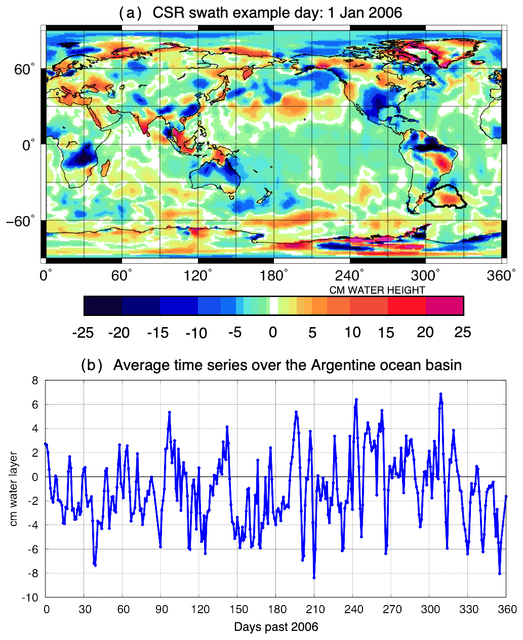
Figure 1 (a) An example day (1 January 2006) of the GRACE swath data. (b) An example of the temporal resolution of the GRACE swath series over the Argentine ocean basin off the coast of Brazil. The thick line in (a) shows the basin outline used.

We also consider a pair of additional GRACE series, ITSG2016 and ITSG2018, created by the Technische Universität Graz (TU Graz; see the “Data availability” section). The older of the two, ITSG2016 (Mayer-Gürr et al., 2016), is being superseded by the newer ITSG2018 (Kvas et al., 2019; Kvas and Mayer-Gürr, 2019). Both series are created in spherical harmonic form to maximum order 40 using Kalman filtering. In order to resolve the daily global gravity field, the solutions are stabilized using a stochastic model derived from geophysical models, along with a priori land–ocean masks (Kurtenbach et al., 2012). ITSG (Institute of Geodesy at Graz University of Technology) data exist even when GRACE does not augment them, but they tend toward the models used, so we omit all days when the CSR swath data denotes a gap. The two ITSG versions differ in the background models used and the details of how instrumental processing steps were handled (see the websites in the “Data availability” section for details). Significantly, ITSG2016 uses the release 5 ocean de-aliasing model (AOD5), while ITSG2018 uses the newer release 6 version (AOD6; see next section).

3.3 De-aliasing ocean models

It is critically important for the production of monthly GRACE gravity products that sub-monthly changes within the ocean that could cause gravitational anomalies are estimated and removed from the GRACE data before processing. Doing so prevents sub-monthly signals from aliasing into the monthly estimates. Even the higher-frequency GRACE series remove these modeled estimates from their input before processing the gravity fields and then restore them later. This means the CSR swath and ITSG solutions considered here actually solve for the residual gravitational signal between the reality and the ocean model. In this paper, we look for evidence that GRACE can see not merely the reproduced a priori model, but also the additional high-frequency ocean signal beyond that.

We will consider the oceanic bottom pressure signals (GAD products) of the two most recent GRACE Atmosphere and Ocean De-aliasing (AOD) models, AOD release 5 (Dobslaw et al., 2013; Flechtner et al., 2014) and AOD release 6 (Dobslaw et al., 2017). These ocean bottom pressure products are the output of high-resolution baroclinic ocean models and do not predict the influence of tides.

The AOD5 ocean bottom pressure estimates come from the Ocean Model for Circulation and Tides (OMCT) (Thomas, 2002), a baroclinic ocean model that estimates the state along 1^∘ horizontal grids with 20 vertical layers and time steps of 20 min. OMCT is forced every 6 h with the European Centre for Medium-Range Weather Forecasts (ECMWF) atmospheric pressures, wind stresses, temperatures, and freshwater fluxes. Its bottom pressure output is made available for GRACE processing every 6 h with the spatial resolution given by a maximum spherical harmonic order of 100 (∼200 km). The CSR swath and ITSG2016 GRACE series were both made using AOD5.

The bottom pressure estimates of AOD6, the newest GRACE generation de-aliasing product, are instead based on the Max Planck Institute for Meteorology Ocean Model (MPIOM) (Jungclaus et al., 2013), a global general circulation ocean model that is a cousin to OMCT, not a direct descendant. The innate spatial resolution of this model is 1^∘ along the horizontal with 40 vertical layers, and time steps are given as 90 min. It is similarly forced by ECMWF atmospheric pressures, wind stresses, temperatures, and freshwater fluxes, but it outputs every 3 h rather than every 6 and to a maximum spherical harmonic order of 180 (∼111 km).

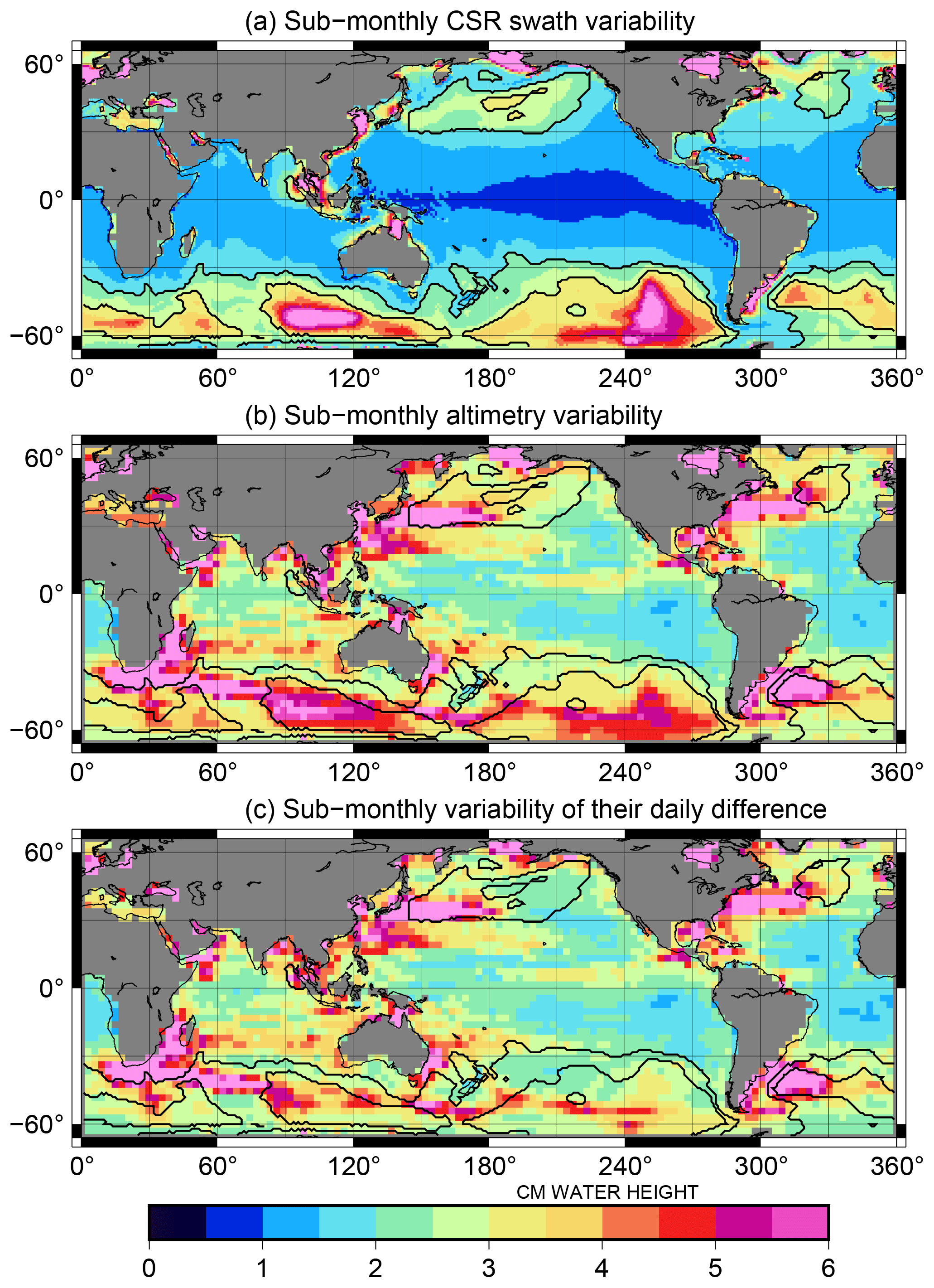
Figure 2 Standard deviation of (a) CSR swath sub-monthly ocean bottom pressure, (b) Jason altimetry sub-monthly sea surface height anomalies, and (c) the difference between the two series during 2002–2016. Units are centimeters of water height in all cases. For comparison's sake, all plots include the 2 and 3 cm contour lines computed from the CSR swath plot (a).

As a comparison, we also briefly consider the high-frequency ocean component of the de-aliasing product used with the Jason altimetry data. A run of the barotropic, nonlinear, finite-element model Mog2D (Carrère and Lyard, 2003; Lynch and Gray, 1979) is used for this, representing the impacts of the ECMWF winds and pressure fields at frequencies with periods below 20 d (note: this is different than the ∼30 d months used elsewhere in this paper). The full dynamic atmospheric correction (DAC) product is unfortunately released as a combination of Mog2D with the larger inverted barometer model, which contains a significant sub-20 d signal as well and thus cannot be easily separated (see the “Data availability” section). However, a separated subset of the high-frequency Mog2D altimetry de-aliasing ocean model is available along the Jason ground tracks within the GDR records themselves, which is what we use here.

4 Sub-monthly results

As an example of the statistics we will be computing, we show the point-by-point standard deviation of the full sub-monthly signal from CSR swath, altimetry, and the difference of CSR swath–altimetry in Fig. 2. This plot, like all others, is computed only over dates when all data types exist, between April 2002 and January 2016. Notice how the altimetry sea level anomaly product shows a very large (> 5 cm water height) variability within the major current systems. GRACE does not see these signals, either because they are short-wavelength signals (for example, eddies) beneath the ∼300 km resolution of GRACE or because they are sea surface height changes that do not correspond to a mass change (for example, those caused by a change in temperature, not pressure). Additionally, there are several areas of high, short-wavelength ocean activity, such as the Argentine gyre southeast of Brazil, where GRACE registers only a reduced fraction of the full signal for the aforementioned reasons.

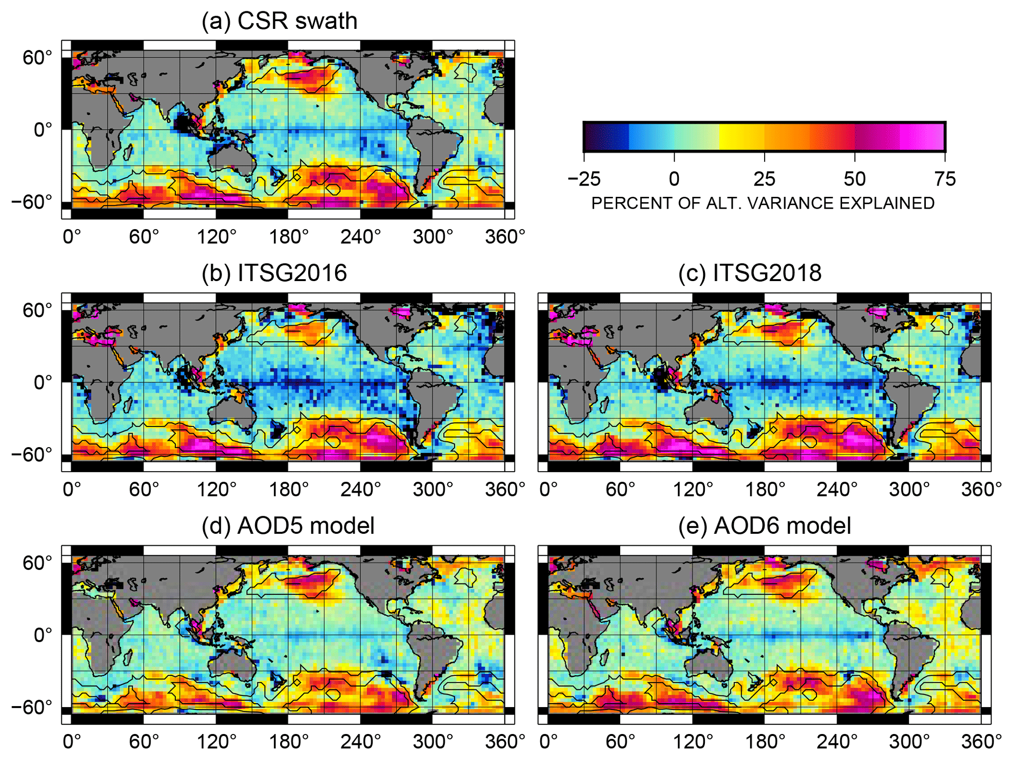
Figure 3 Percent of altimetric variance explained by five different series: (a) CSR swath GRACE data, (b) ITSG2016 GRACE data, (c) ITSG2018 GRACE data, (d) AOD5 ocean de-aliasing model, and (e) AOD6 ocean de-aliasing model.

It may appear at first glimpse that GRACE does not measure a sufficient altimetric signal to allow our technique to work, but that is a trick of the eye. Figure 3a shows the percent of the altimetry sub-monthly variability explained by the GRACE swath series. This percent of variance explained (PVE) is closely related to the normalization of Fig. 2c found by dividing through by Fig. 2b and can be computed as

$$\begin{array}{}\text{(4)}& \mathrm{PVE}=\left(\mathrm{1}-{\displaystyle \frac{\mathrm{var}(\text{alt.}-\text{GRACE})}{\mathrm{var}(\mathrm{alt}.)}}\right)\times \mathrm{100}\mathit{\%},\end{array}$$

where obviously signals other than GRACE can be inserted in its place. We see that there are large sections of ocean, particularly the Southern Ocean, where the CSR swath series explains 25 %–75 % or more of the altimetry sub-monthly variability. It does not explain the variability within the equatorial region simply because there is so little signal there (see Fig. 2) that the signal-to-noise ratio becomes very low. The altimetric PVEs by ITSG2016 and ITSG2018, and by the de-aliasing models GAD5 and GAD6, are shown in direct comparison in Fig. 3. In each case, the largest PVEs occur in about the same areas as in the CSR swath series, with only the relative amplitude changing. Generally, with the exception of the northern Atlantic, the three high-frequency GRACE series show a higher PVE compared to altimetry than either of the GRACE de-aliasing models.

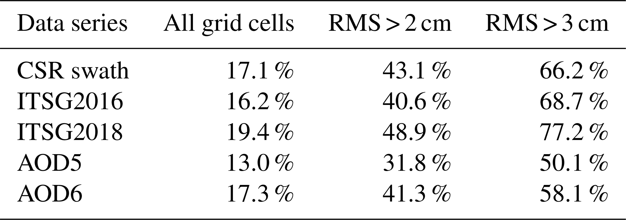
Table 1 lists the areal percentage of the ocean between 66^∘ S and 66^∘ N for which each series explains at least 25 % of the altimetry variance. The first data column shows this statistic for all grid cells, while the last two columns consider only those non-coastal cells in which the CSR swath series measures a root mean square (RMS) variability of at least 2 or 3 cm water height (masks outlined in Fig. 2a). All three of the GRACE series show a large negative PVE (< −25 %) near 90^∘ E, 5^∘ N (Fig. 3a, b, c). This solid-Earth signal is the impact of the Andaman–Sumatra earthquake from 2004, which had a large gravitational effect both during and after the event. For statistical purposes, we have removed the most affected grids from our analysis in all of the following tables.

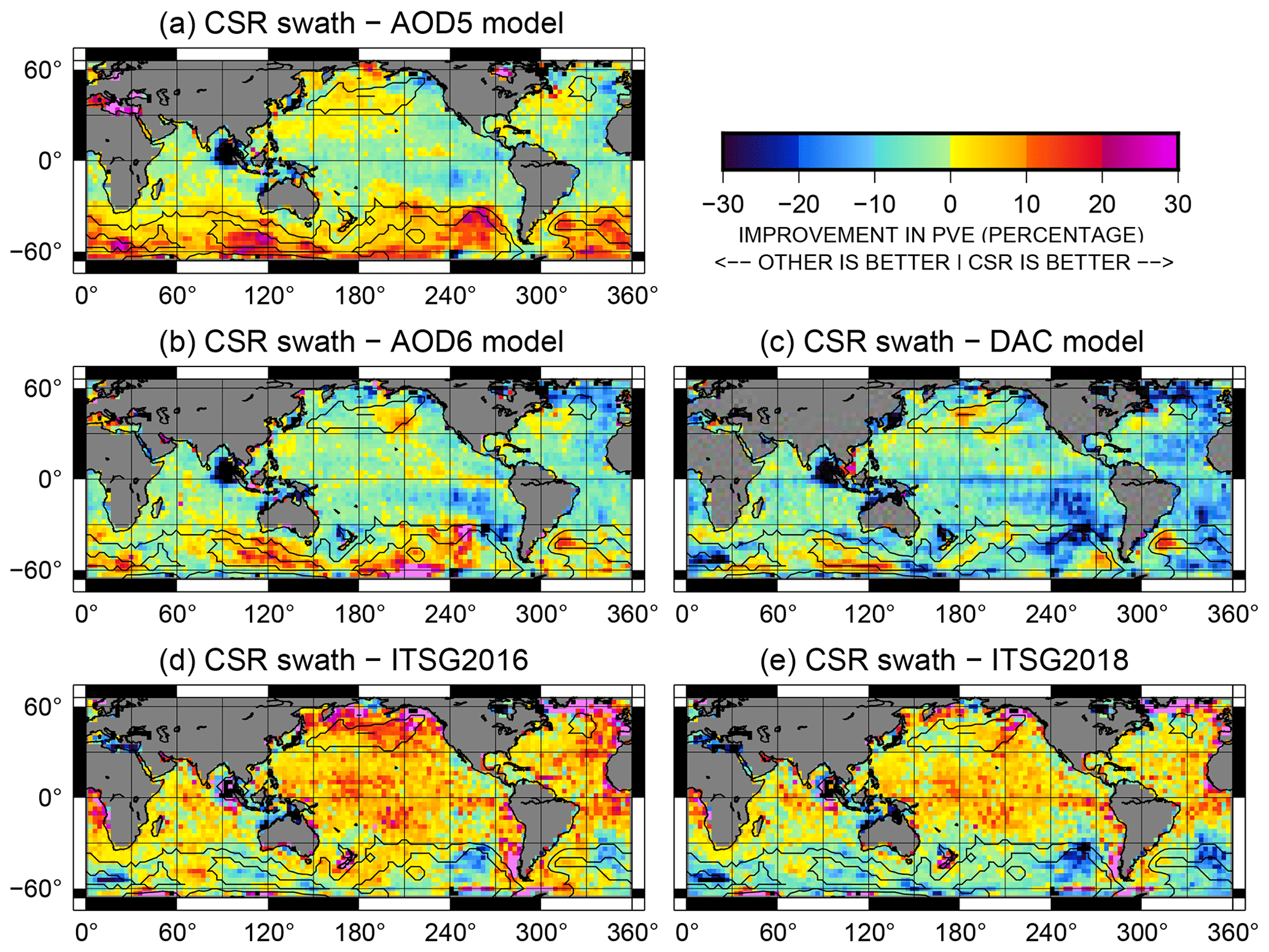
Figure 4 Differences in sub-monthly PVE for CSR swath vs. another data type: (a) AOD5 de-aliasing ocean model, (b) AOD6 de-aliasing ocean model, (c) altimetry DAC de-aliasing ocean model, (d) ITSG2016 GRACE data, and (e) ITSG2018 GRACE data. Values are relative to CSR swath PVEs, so positive numbers (red) denote that the CSR swath matches altimetry better, while negative numbers (blue) denote that the other series matches altimetry better.

Table 1 Percent of non-coastal ocean area explaining at least 25 % of the altimetry sub-monthly variance. The 2 and 3 cm RMS bounds are defined in Fig. 3a.

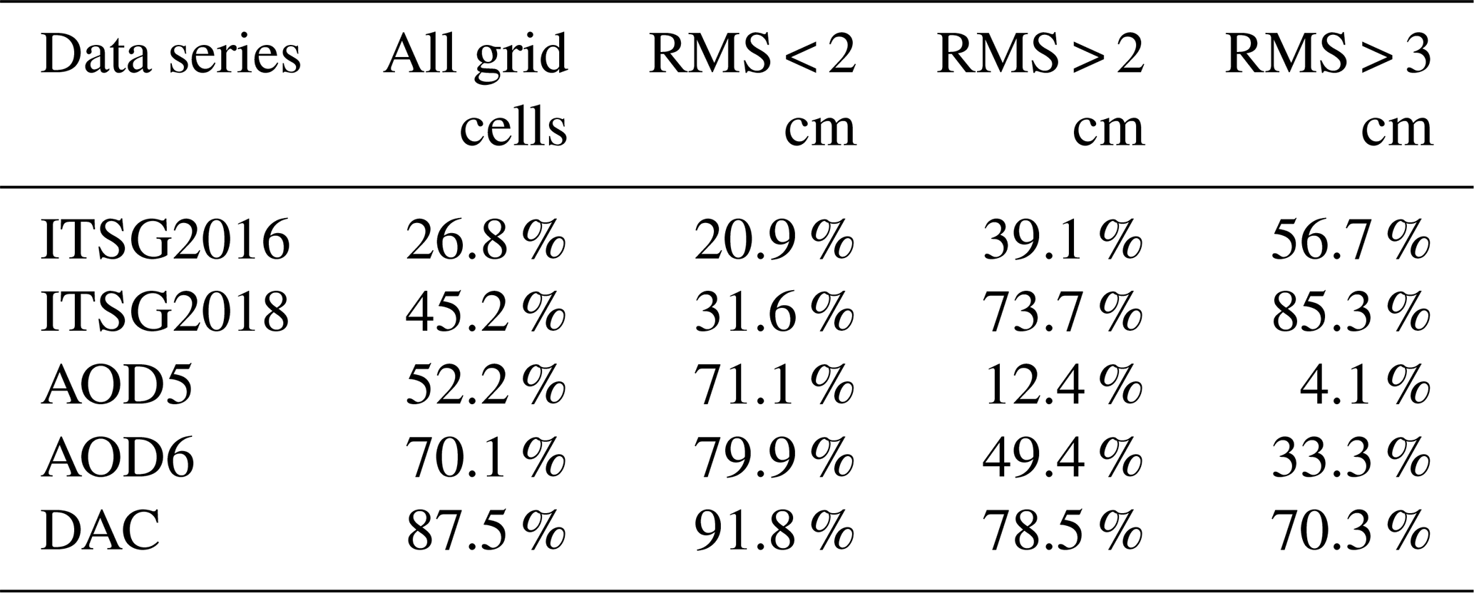
The double-difference plots (Fig. 4) obtained by subtracting one map in Fig. 3 from another via Eq. (3) can better show us which data series most closely matches altimetry in the sub-monthly realm. The percentage of negative non-coastal ocean area between 66^∘ S and 66^∘ N is listed in Table 2. These percentages measure the area where each alternative series explains more of the altimetry variance than the CSR swath series does – or, in other words, places where the alternative series is more likely than CSR swath to be correct. The statistics are again given for all grid cells as well as for the low-signal and high-signal areas separately. They again omit the earthquake area and coastal regions that might contain ice or hydrological leakage effects.

We use the CSR swath series as our main comparison series here. We immediately note that the CSR swath series is, in nearly all higher-latitude locations, better than the AOD5 model upon which it was based. Figure 4a is clear proof that the CSR swath series is not merely regurgitating the a priori ocean model provided to it but is altering it in a manner that makes it more like altimetry – a manner very likely to be an improvement.

Table 2 Percent of non-coastal ocean area where the altimetric variance is better explained by the given time series than by the CSR swath series. The 2 and 3 cm RMS bounds are defined in Fig. 3a.

By comparing Fig. 4b to a, we see that, in most places, the newer AOD6 model improves upon AOD5, making the differences between it and the GRACE CSR swath series smaller. However, this is surprisingly not true within one region, near 210^∘ E, 60^∘ S. In the bright-pink-colored region there, the AOD6 model is found to be both different from the CSR swath series and measurably worse based on the altimetric PVE. To confirm that this difference was not caused by an error in the altimetry product, we also ran the same analysis on the high-frequency ocean de-aliasing model used by Jason altimetry (Fig. 4c). We found that the CSR swath series is roughly equivalent to the Jason ocean de-aliasing model in that spot. This implies that GRACE, AOD5, and the Jason de-aliasing model all estimate one signal, which additionally matches the altimetry data, while the AOD6 model predicts something very different. Presumably the AOD6 model is wrong, though precisely why was not immediately clear.

Figure 5 Example time series (a) and spectral amplitude plot over the AOD6 anomalous spot (near 210^∘ E, 60^∘ S), with lines offset for clarity. Spectral analysis (b) was computed for the time span 2003–2013. The black line shows the uncertainty for the CSR swath series (which is similar to the AOD5 and altimetry uncertainties), and the grey line shows the uncertainty for the AOD6 series. Signals below these lines are not statistically significant.

We examined whether an error over a limited time period was causing the AOD6 discrepancy but found that the same patch of poorly matched data occurred for all years from 2003 to 2016. Figure 5b shows the regionally averaged sub-monthly time series of AOD5, AOD6, and CSR swath over a single year compared to the sea level anomalies from Jason altimetry. The time series of all four series are very similar, with altimetry being the most unlike the other three, as might be expected. The correlation between CSR swath and AOD5 time series is 94.2 %, while the correlation between CSR swath and AOD6 is still high at 91.6 %. However, the main difference is not a matter of correlation but of amplitude: AOD6 is magnified compared to AOD5. The standard deviation of the CSR swath series over 2003–2013 is 3.72 cm, which corresponds well with the AOD5 standard deviation of 3.75 cm. The AOD6 time series has a much higher standard deviation than either: 5.33 cm.

We then ran a spectral analysis of the four time series over the mostly continuous 2003–2013 time span (Fig. 5a) using the least-squares-based Lomb–Scargle method to accommodate the remaining gaps in the data. From this we learned that the AOD6 differences are not caused by a change at a single harmonic but are rather an amplified signal throughout the entire sub-monthly band, particularly at periods below 10–15 d. The root cause of this difference was initially unknown, though the comparison with altimetry strongly suggested that the AOD6 data were in error in this region. This assessment has since been provided to the developers of AOD1B, who hypothesize that the problem may be caused by a deficit in the MPIOM ocean model configuration around Ross Sea. In AOD6, the model treats all ice shelf areas as land, whereas in fact water several hundreds of meters deep is present underneath the floating ice. In the next release 07 of AOD1B, ice shelf areas will be included in the ocean model domain, which is expected to have a positive effect on the simulation of the region's dominant eigenmodes at 3 to 8 d periods, thus hopefully correcting this problem.

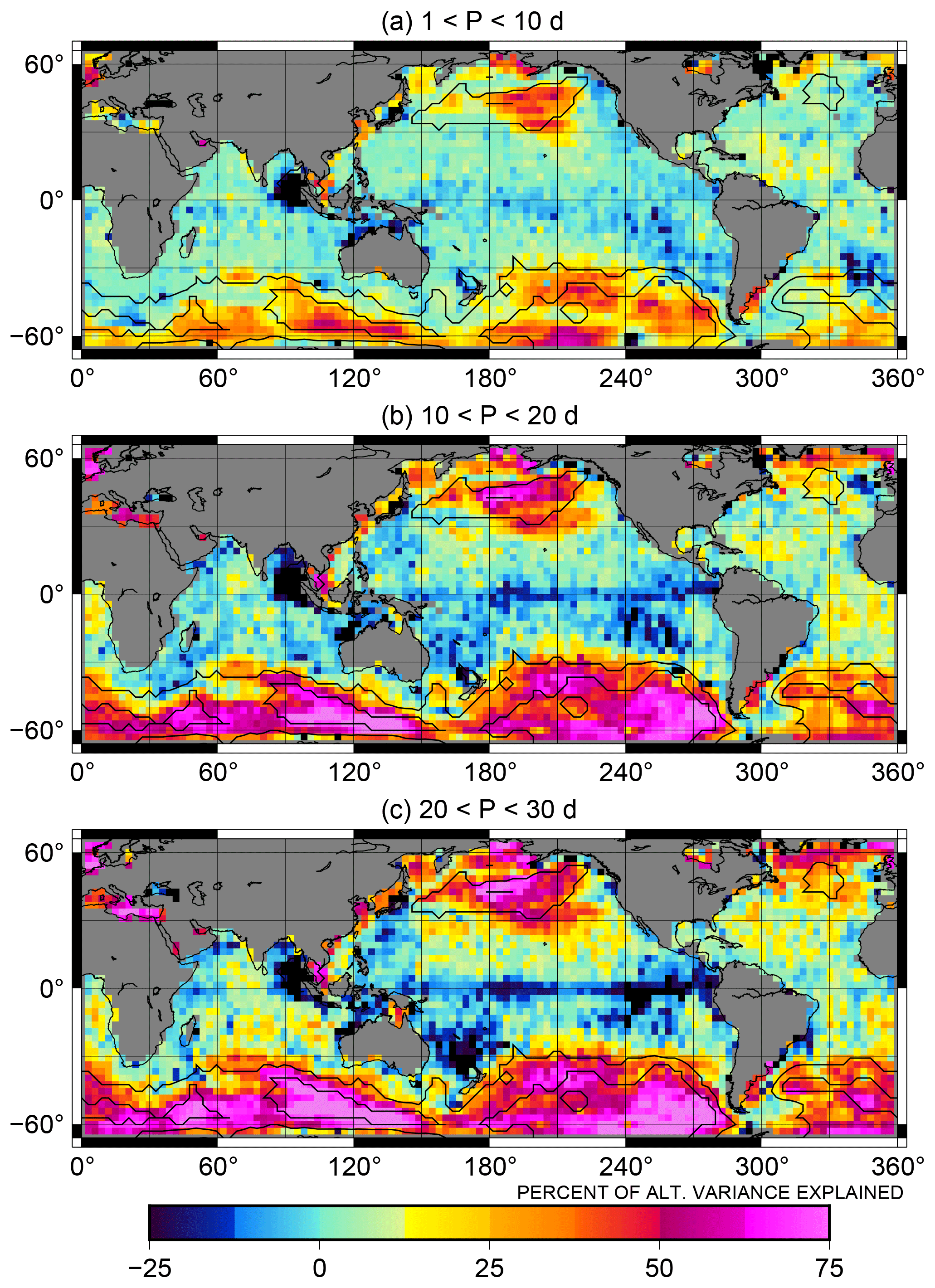
Figure 6 Percent of altimetric variance explained by the CSR swath series at three sub-monthly frequency bands: (a) periods below 10 d, (b) periods between 10 and 20 d, (c) periods between 20 and 30 d.

We also compared the CSR swath series to the two ITSG high-frequency GRACE series (Fig. 3d and e). The older ITSG2016 series is generally less like altimetry than the CSR swath series, particularly in the equatorial and northern oceans. Only 26.8 % of the ocean area shows an improvement relative to altimetry when switching from CSR swath to ITSG2016. The newer ITSG2018 series is decidedly better, with 45.2 % of the grids improving over CSR swath, including 73.7 % of the area with more than 2 cm RMS GRACE variability. ITSG2018 is likely an improvement over the CSR swath series in the Southern Ocean, while CSR swath is probably still better in the equatorial and quieter northern parts of the ocean. Larger differences for both ITSG series along some coasts suggest either worse tidal models or (particularly near Greenland) significantly increased leakage from nearby land in comparison to the CSR swath series. We also anticipate the arctic and near-Antarctic oceans to be more poorly measured by ITSG2018 than CSR swath because of the large impact of ice leakage in those areas, but that cannot be tested using the nonpolar Jason altimetry data.

5 Band-passed results

We used a set of Gaussian temporal windows to act as band-pass filters, dividing the above results into three pieces: signals with periods below 10 d, between 10 and 20 d, and between 20 and 30 d. To create the band-pass effect, we used three high-pass filters with 10, 20, and 30 d cutoffs, then subtracted one from the other in subsequent pairings. (For example, the 20–30 d band-pass signal is the 30 d high-pass signal minus the 20 d high-pass signal.) To provide a baseline, Fig. 6 shows the altimetric PVE by the CSR swath series for each frequency band. For signals with periods of more than 10 d, the CSR swath series perceives at least 25 % and often more than 50 % of the altimetric variability across most of the Southern Ocean and the high-signal part of the north Pacific. Conversely, the swath series does a poor job of reproducing the altimetry signal at periods shorter than 10 d. Since most of the altimetric signal in this highest-temporal-frequency band occurs over small spatial scales along the major currents, it is not surprising that GRACE cannot measure it.

Table 3 Percent of non-coastal ocean area where the altimetric variance is better explained by the given time series than by the CSR swath series. The 2 cm RMS bounds are defined in Fig. 3a. Column 5 estimates only over the parts of those regions that are in the Southern Ocean.

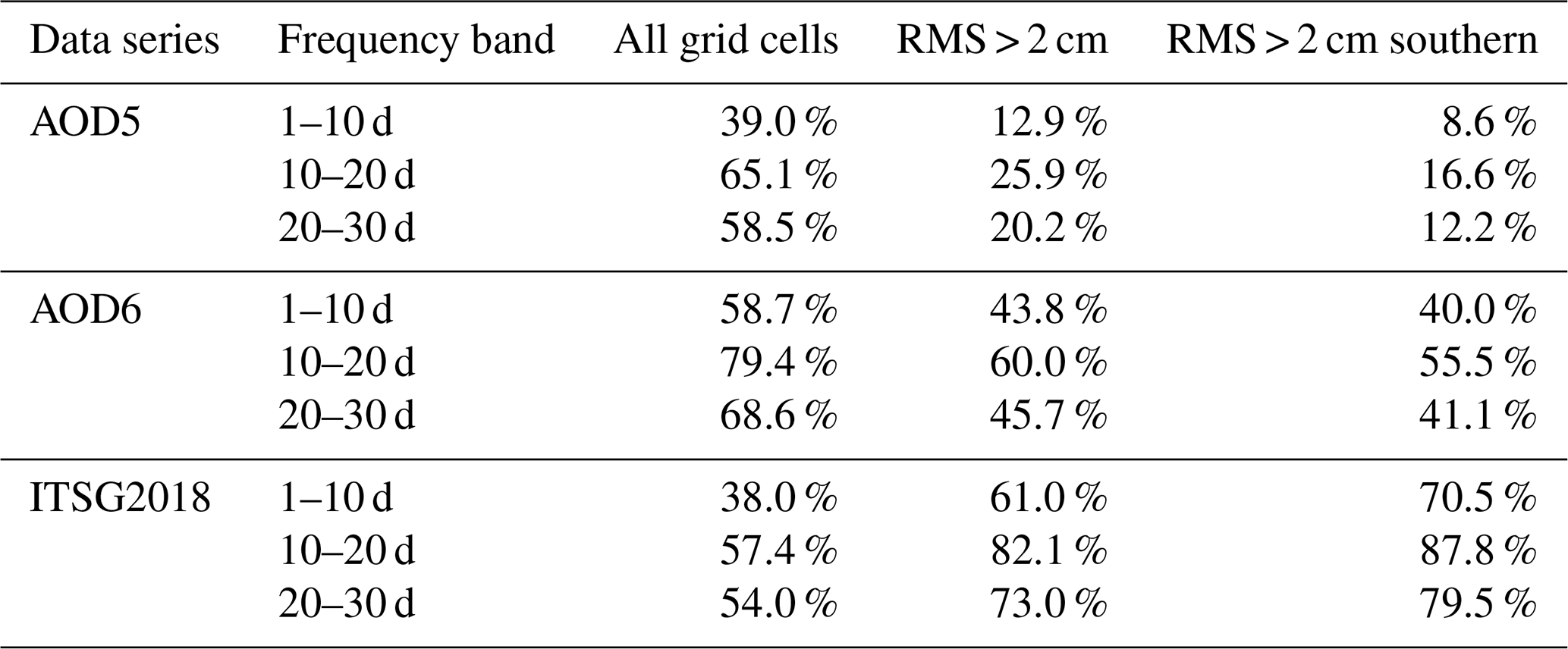
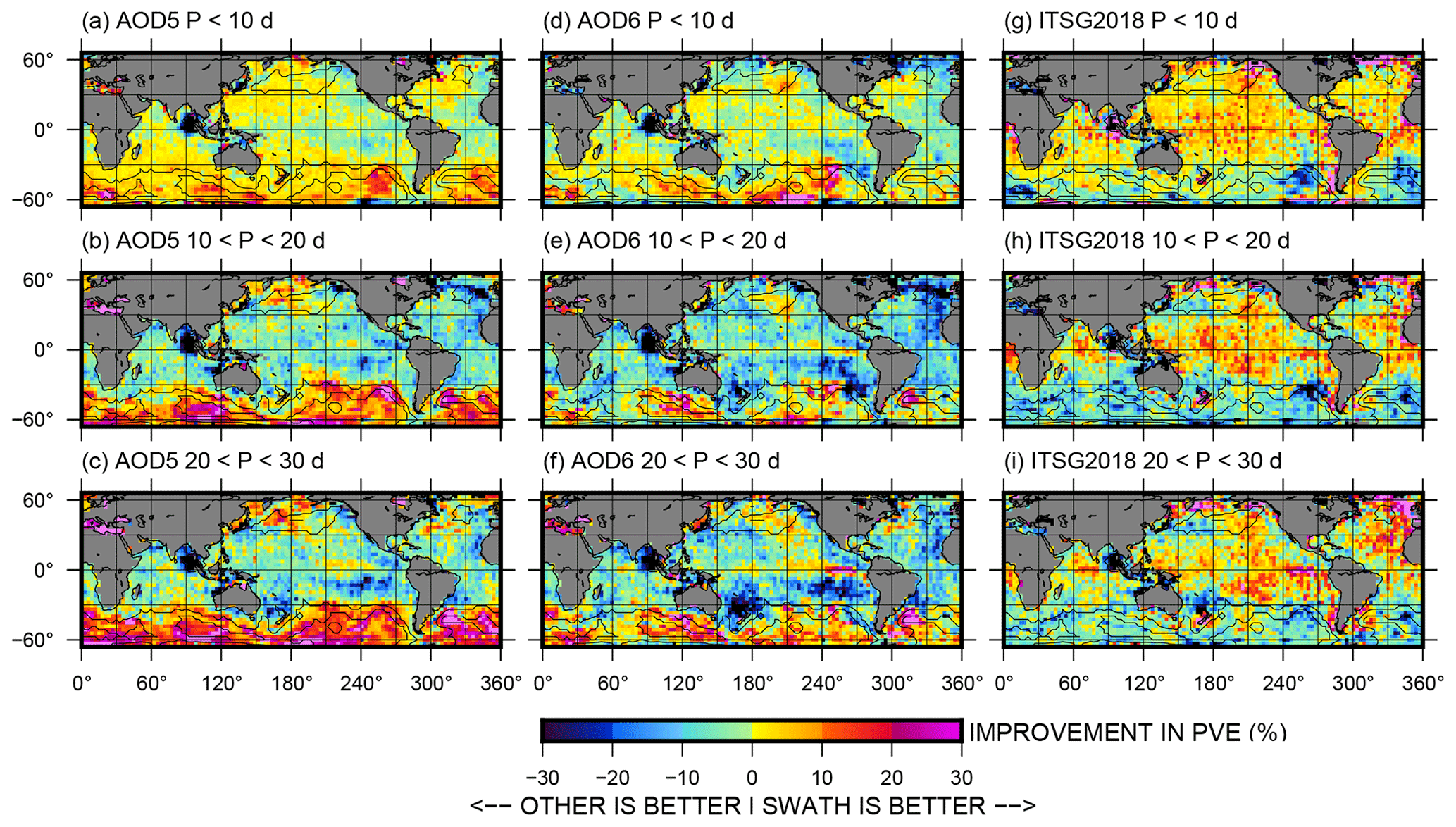
Figure 7 Differences in PVE for CSR swath vs. another data type per frequency band: (a, b, c) AOD5 de-aliasing ocean model, (d, e, f) AOD6 de-aliasing ocean model, and (g, h, i) ITSG2018 GRACE data. Panels (a, d, g) give the highest sub-monthly frequency band, while panels (c, f, i) give the lowest sub-monthly frequency band. Values are relative to CSR swath PVEs, so positive numbers (red) denote that the CSR swath matches altimetry better, while negative numbers (blue) denote that the other series matches altimetry better.

Figure 7 shows the double-difference PVE comparison for the three frequency bands, with statistics given in Table 3. Its left-hand column depicts the CSR swath series minus AOD5 results, demonstrating that the CSR swath series estimates an improved ocean signal across the entire Southern Ocean in all three frequency bands, especially for signals with periods longer than 10 d. In the 10–20 d band, the CSR swath series better explains the altimetric signal than its a priori model can in 83.4 % of the high-signal (RMS > 2 cm) part of the Southern Ocean. In the 20–30 d band, that improves to 87.8 %.

The middle column of Fig. 7 shows the same thing, but for AOD6. For periods shorter than 10 d, the two series are roughly equivalent. For sub-monthly periods longer than 10 d, the AOD6 series better matches altimetry over northern and equatorial regions, while the CSR swath series proves to be 10 % or more better than AOD6 in much of the Southern Ocean. Improvements over its AOD5 predecessor can be seen in all frequency bands. The CSR swath series better explains the 10–20 d altimetric signal than the AOD6 model in 44.5 % of the high-signal Southern Ocean bins. For the 20–30 d band, CSR swath better explains 58.9 % of these bins. Additionally, the small region of poor performance near 210^∘ E, 60^∘ S is confirmed to be a very-high-frequency issue, mainly visible in the 1–10 d band and not visible in the 20–30 d band.

The right-hand column of Fig. 7 is the ITSG2018 comparison. (ITSG2016 was found to be inferior to its successor in all bands, so we do not depict it here.) There are few frequency-based distinctions between the CSR swath and ITSG2018 series. In the Southern Ocean, ITSG2018 signals with any sub-monthly period are more likely than CSR swath signals to be like altimetry (ITSG2018 is better in 65.5 %, 85.6 %, and 79.4 % of the grids by area for the 0–10, 10–20, and 20–30 d bands, respectively). The opposite is true in the lower-signal equatorial and northern oceans (similar percentages of 26.0 %, 45.2 %, and 44.7 %). The large positive (> 30 %) coastal differences near Alaska, Patagonia, the Antarctic Peninsula, and Greenland again suggest that ITSG2018 does not segregate the land ice leakage as well as the CSR swath series does, while the large negative (< −30 %) coastal differences north of Australia hint towards a possibly improved tidal or ocean model. The CSR swath series generally higher equatorial PVE could indicate that the series has better reduced the GRACE stripe-like errors compared to ITSG2018 in these regions of relatively low oceanographic signal.

6 Conclusions

Using a comparison with Jason altimetry, we have demonstrated that two modern near-daily GRACE series are capable of estimating the real sub-monthly oceanographic signal. Both the CSR swath series and ITSG2018 explain a fair proportion of the high-frequency altimetric signal outside of major currents, the equatorial region, and the northern Atlantic, which is more of it than the a priori ocean models they are based upon can explain. We found that these near-daily GRACE series are particularly sensitive for signals with periods above about 10 d and less so as the signal length shortens below that.

At the moment, it appears that the CSR swath series is better able to eliminate land leakage from ice and hydrology entering the ocean grids, making it distinctly better than ITSG2018 along the coasts and near the large ice sheets. CSR swath also appears probably better at removing the false north–south stripes commonly created during GRACE processing, allowing the quieter equatorial regions to be better estimated. The ITSG2018 series, on the other hand, appears to better observe the sub-monthly state of the Southern Ocean, particularly in those areas with large amounts of variability. This might be an impact of the different processing scheme, or it might be due to the use of the newer AOD6 model as an ocean de-aliaser. To test the latter, we plan on eventually reproducing the CSR swath data with AOD6 as an a priori model.

Our analysis here demonstrates that, particularly in the poorly observed Southern Ocean, sub-monthly GRACE data can be used to improve our knowledge of the ocean bottom pressure. We hope to use this in the future to validate global ocean models, perhaps even merging the GRACE data with modeled results in order to produce a combined de-aliasing product superior to either source alone.