the Creative Commons Attribution 4.0 License.
the Creative Commons Attribution 4.0 License.
 | 02 Apr 2020
Variability of the thermohaline structure and transport of Atlantic water in the Arctic Ocean based on NABOS (Nansen and Amundsen Basins Observing System) hydrography data
Nataliya Zhurbas
Natalia Kuzmina
Conductivity–temperature–depth (CTD) transects across continental slope of the Eurasian Basin and the St. Anna Trough performed during NABOS (Nansen and Amundsen Basins Observing System) project in 2002–2015 and a transect from the 1996 Polarstern expedition are used to describe the temperature and salinity characteristics and volume flow rates (volume transports) of the current carrying the Atlantic water (AW) in the Arctic Ocean. The variability of the AW on its pathway along the slope of the Eurasian Basin is investigated. A dynamic Fram Strait branch of the Atlantic water (FSBW) is identified in all transects, including two transects in the Makarov Basin (along 159∘ E), while the cold waters on the eastern transects along 126, 142, and 159∘ E, which can be associated with the influence of the Barents Sea branch of the Atlantic water (BSBW), were observed in the depth range below 800 m and had a negligible effect on the spatial structure of isopycnic surfaces. The geostrophic volume transport of AW decreases farther away from the areas of the AW inflow to the Eurasian Basin, decreasing by 1 order of magnitude in the Makarov Basin at 159∘ E, implying that the major part of the AW entering the Arctic Ocean circulates cyclonically within the Nansen and Amundsen basins. There is an absolute maximum of θmax (AW core temperature) in 2006–2008 time series and a maximum in 2013, but only at 103∘ E. Salinity S(θmax) (AW core salinity) time series display a trend of an increase in AW salinity over time, which can be referred to as an AW salinization in the early 2000s. The maxima of θmax and S(θmax) in 2006 and 2013 are accompanied by the volume transport maxima. The time average geostrophic volume transports of AW are 0.5 Sv in the longitude range 31–92∘ E, 0.8 Sv in the St. Anna Trough, and 1.1 Sv in the longitude range 94–107∘ E.
- Article
(6256 KB) - Full-text XML
- BibTeX
- EndNote


Atlantic water (AW) enters the Eurasian Basin in two branches (see, e.g., Aagaard, 1981; Rudels et al., 1994, 1999, 2006, 2015; Schauer et al., 1997, 2002a, b; Berzczynska-Möller et al., 2012; Rudels, 2015; Dmitrenko et al., 2015; Pnyushkov et al., 2015, 2018b): one branch originates from the Greenland and Norwegian seas and flows to the basin through Fram Strait (the Fram Strait branch of the Atlantic water, hereinafter the FSBW), and the other reaches the deep part of the Arctic Ocean near St. Anna Trough after passing through the Barents Sea (the Barents Sea branch of the Atlantic water, hereinafter the BSBW). After entering the Eurasian Basin the FSBW moves eastward with a subsurface boundary current and has a core of higher temperature and salinity than the BSBW. In the longitude range of 80–90∘ E, it encounters and partially mixes with the BSBW, which is strongly cooled due to mixing with shallow waters of the Arctic shelf seas and atmospheric impact (Schauer et al., 1997, 2002a, b). Further, the water masses resulting from the interaction of the two branches spread cyclonically in the Eurasian Basin.
Within the NABOS (Nansen and Amundsen Basins Observing System) project (Polyakov et al., 2007) a unique volume of conductivity–temperature–depth (CTD) data was collected: more than 30 sections were made in various regions of the Arctic Basin in summer and fall 2002–2015. A number of sections in different years were made in the same regions of the basin, which allows studying the interannual variability of the water masses thermohaline structure and the geostrophic volume flow rate in these areas.
The main goal of this work is to investigate the spatial and temporal variability of the AW geostrophic volume flow rate during its propagation along the continental slope of the Eurasian Basin. We further discuss the thermohaline structure and transformation of the FSBW and BSBW. The estimates of the AW transport are sensitive to the temperature and salinity ranges used for the identification of this water (Pnyushkov et al., 2018b), and mixing of FSBW, BSBW and surrounding waters may change the AW geostrophic volume transport along the slope.
We used data from the CTD transects across the slope of the Eurasian Basin in the longitude range of 31–159∘ E measured in the years 2002–2015 within the framework of the NABOS project (in total 39 transects). The data are freely available at the site http://nabos.iarc.uaf.edu (last access: 24 January 2019, IARC, 2019). In addition, a CTD transect across the entire Eurasian Basin and over the Lomonosov Ridge starting at 92∘ E at the slope from R/V Polarstern in 1996 (hereafter PS96) was also included. The locations of the CTD transects are shown in Fig. 1. Most of the transects are aligned cross-slope and grouped at longitudes of 31, 60, 90, 92, 94, 96, 98, 103, 126, 142, and 159∘ E. Four of the 40 transects crossed zonally the St. Anna Trough (at the latitude of 81, 81.33, 81.42, and 82∘ N) through which the BSBW enters the Eurasian Basin. Most of the CTD casts covered the upper layer from the sea surface to either 1000 m depth or to the bottom (if the total depth was shallower). Approximately every third or fourth cast was down to the sea bottom even if the sea depth exceeded 1000 m.
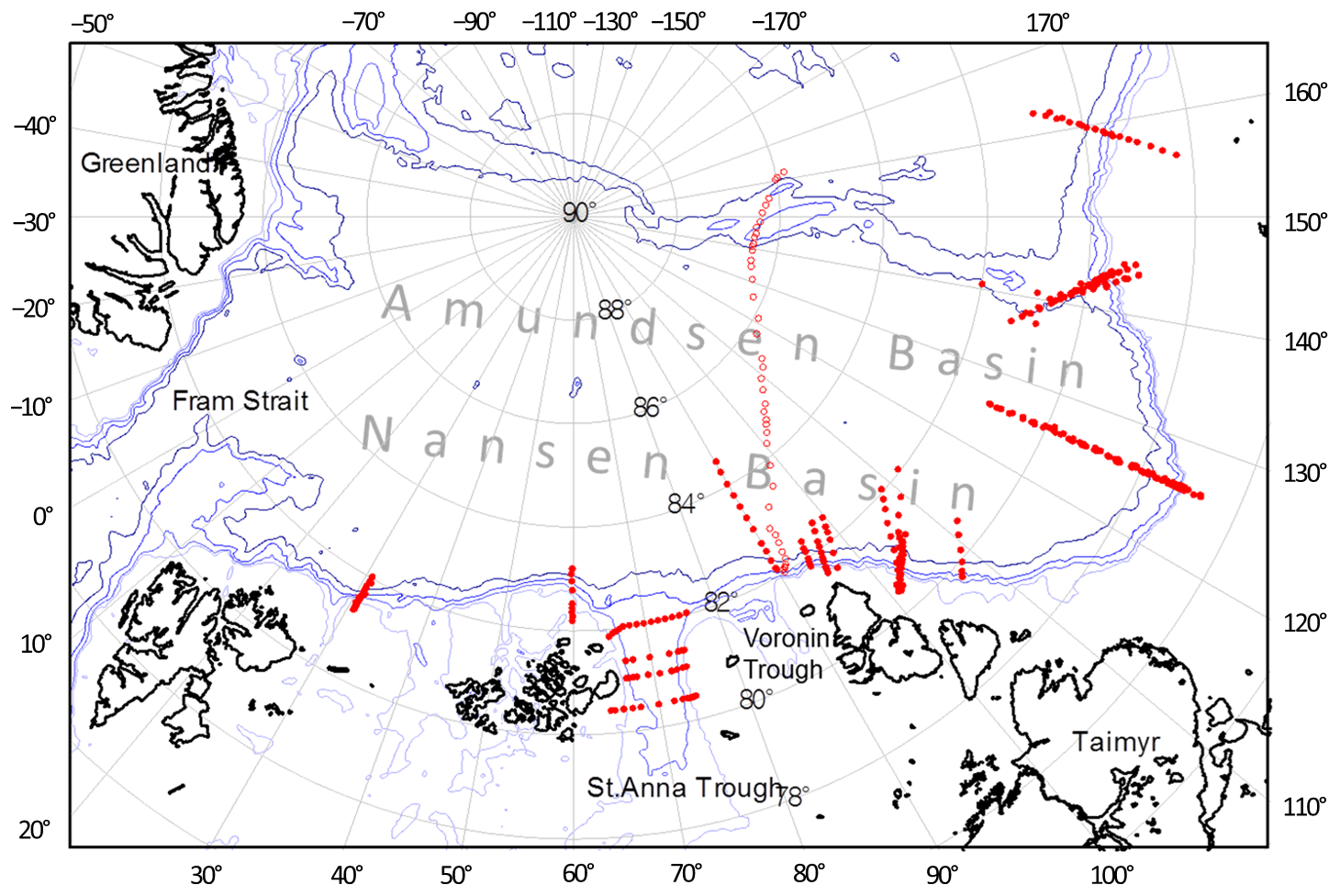
Figure 1Bathymetric map of the Eurasian Basin with 300, 500, 1000, and 2000 m contours shown. The red filled and blank circles are the locations of CTD stations on the NABOS and PS96 transects, respectively.
To estimate the volume transport of the Atlantic water, we applied standard dynamical method. The no-motion level (the depth of zero velocity) was determined from the following consideration. If the baroclinic current occupies the upper layer or/and some intermediate layer, the no-motion level can be chosen in a calm deep layer (where the horizontal density gradient is relatively small). By contrast, in case of a near-bottom gravity flow, the no-motion level can be reasonably chosen well above the near-bottom flow. For the level of no-motion, we adopted either 1000 m depth or the sea bottom depth, if the latter was smaller than 1000 m for the FSBW, and approximately 50 m, where density contours were more or less flat, for the observations of BSBW in the St. Anna Trough (see also below).
Since the FSBW brings saline and warm water to the Eurasian Basin, the geostrophic transport was found by integration over the depth range with positive temperature, θ>0 ∘C, and relatively high salinity, S>34.5 (the salinity is given in the practical salinity scale); that is, near-surface layers with warm and fresh water (which cannot be attributed to AW) were excluded. For the observations of BSBW in the St. Anna Trough the geostrophic transport was calculated by integration over a depth range with temperature below 0 ∘C and salinity above 34.5. If both AW branches were present on the transect, the integration was performed over the entire depth range but excluding the cold near-surface layer (θ<0 ∘C) and the warm (θ>0 ∘C) and relatively fresh (S<34.5) near-surface layer. The zero-velocity depth in this case was chosen after inspection of the observed pattern of density contours, i.e., suggesting either the near-surface flow pattern or the near-bottom flow pattern (see Sect. 3). The details and limitation of the geostrophic velocity calculations are discussed in Zhurbas (2019).
3.1 Variability of the thermohaline pattern on the AW pathway along the slope of the Eurasian Basin
3.1.1 CTD transect analysis
The transformation of thermohaline signatures (i.e., patterns of salinity S, potential temperature θ, and potential density anomaly σθ vs. cross-slope distance and depth) of the AW flow on its pathway along the slope of the Eurasian Basin are presented in Fig. 2. The σθ contours in transects at 31∘ E diverge towards the continental slope margin (to the south), shallowing above the warm and saline core of the AW and sloping down beneath it associated with a eastward subsurface flow. Such a distribution of isopycnic surfaces was observed on all NABOS transects taken across an available continental slope at 31∘ E. According to Fig. 2 the warm and saline core of the Fram Strait branch of the AW with the maximum temperature θmax of 4.88 ∘C at the depth m and the maximum salinity Smax of 35.11 at the depth m is found on the slope at about 1000 m isobath.

Figure 2Temperature θ, salinity S, and potential density anomaly σθ vs. cross-slope distance and depth for the NABOS08 transect across the Eurasian Basin slope at 31∘ E. Locations of the CTD stations are shown in the transects at the top. Here and hereinafter the NABOS expedition references are abbreviated: for example NABOS08 corresponds NABOS-2008.
Figure 3 presents temperature, salinity, and potential density for two zonal transects across the St. Anna Trough at latitudes of 81 and 82∘ N. A stable pool of cold (θ<0 ∘C) and dense (σθ>28 kg m−3) water in the bottom layer is seen adjacent to the eastern slope of the trough. The transfer of the densest water pool to the eastern slope corresponds to a geostrophically balanced near-bottom gravity flow to the north. This near-bottom gravity current also carries waters of Atlantic origin, which are strongly cooled due to mixing with shelf waters in the Barents and Kara seas. Above the near-bottom gravity flow of the BSBW one can observe a two-core structure of warm FSBW with temperature up to 2.5 ∘C that enters the St. Anna Trough from the northwest at the western side of the trough and leaves it for the northeast at the eastern side of the trough. At 82∘ N, the BSBW overflows a ridge-like elevation east of the St. Anna Trough (Fig. 3a–c). Studies of the currents and hydrography in the St. Anna Trough can be found in Schauer et al. (2002a, b), Rudels et al. (2015), and Dmitrenko et al. (2015).
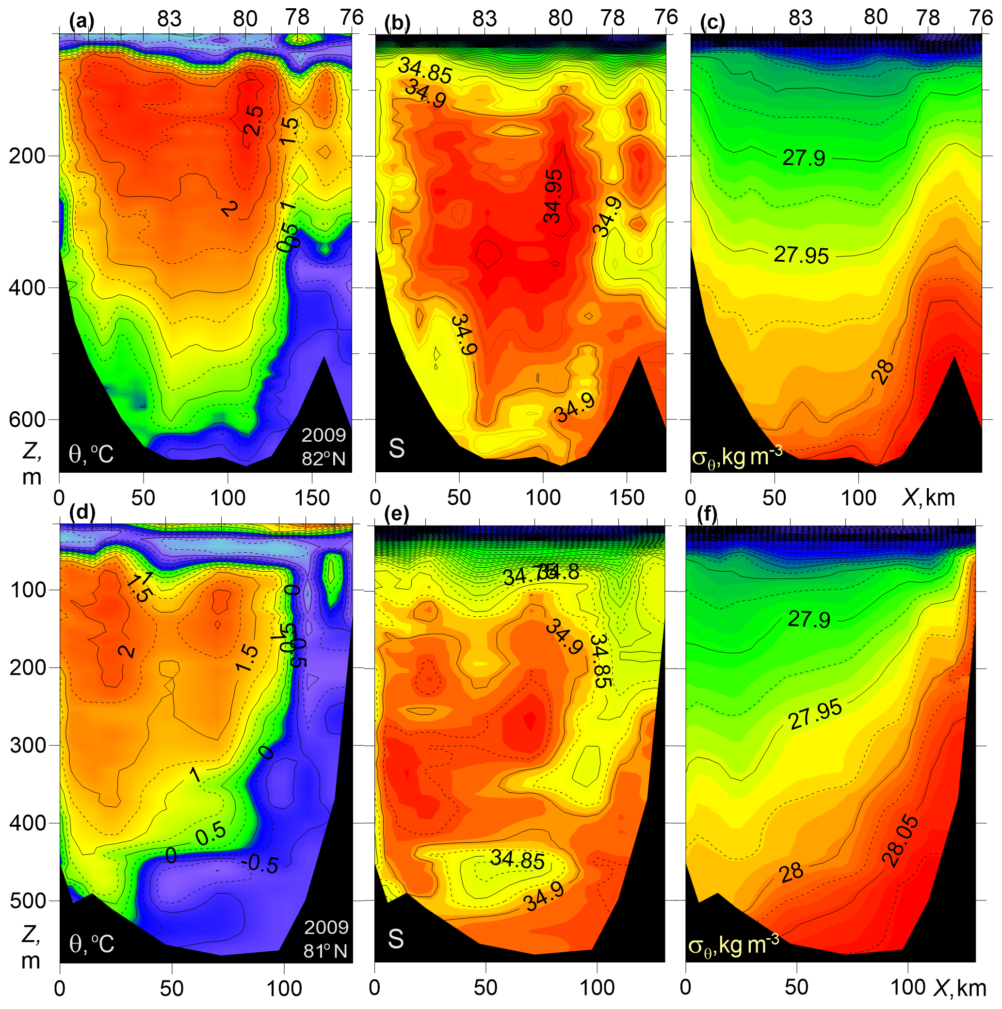
Figure 3Temperature θ, salinity S, and potential density anomaly σθ vs. distance and depth for zonal transects across the St. Anna Trough at latitudes of 81∘ N (d–f, NABOS09) and 82∘ N (a–c, NABOS09). The x axis is directed to the east. Numbers at the top indicate numbers of the CTD stations.
In order to understand the effect of the FSBW and the BSBW transformation on geostrophic volume flow rate, it is necessary to identify water masses of different origin. For that purpose the following criterion is often used (Walsh et al., 2007; Pfirman et al., 1994): the water masses of the FSBW are characterized by θ>0 ∘C, and the BSBW can be identified by ∘C, , and kg m−3. Other approaches to define BSBW are given in Schauer et al. (1997, 2002a, b) and Dmitrenko et al. (2015). According to Schauer et al. (1997, 2002a, b) the BSBW includes all waters that enter the Nansen Basin from the St. Anna and Voronin troughs. The temperature of these waters, however, can reach ∼1 ∘C. The justification for this approach was based on θ–S analysis of the waters of the northeastern part of the Barents Sea and the St. Anna and Voronin troughs. According to Dmitrenko et al. (2015), the BSBW consists of two water masses, and the temperature of the warmer water mass can only slightly exceed 0 ∘C (for more details, see Sect. 3.1.2). Here we will rely on the definitions of the FSBW and BSBW proposed by Dmitrenko et al. (2015).
In Fig. 4 the CTD transect at 92∘ E carried out in the 1996 Polarstern expedition just east of the entrance point of the BSBW to the Eurasian Basin from the St. Anna Trough and Voronin Trough is presented. It can be assumed that a part of the BSBW extends deep into the basin, mixing with the FSBW, while another part of the BSBW flows eastward along the slope according to the general cyclonic circulation observed in the Eurasian Basin. On the presented transect the BSBW is observed in the depth range below 600 m as a narrow, about 10 km wide strip of cold water near the slope (see also Sect. 3.1.2) adjacent to a 300 km wide zone occupied by the warm FSBW. The potential density distribution of FSBW in this transect is similar to transects at 31∘ E. That is to say, despite the masking effect of vertical undulations of σθ contours caused by internal waves and mesoscale eddies (one of subsurface, intra-pycnocline eddies is probably identified at the distance of Y=510 km), isopycnals tend to shoal or deepen above or below the FSBW core towards the continental slope margin (to the south) which, in terms of geostrophic balance, implies the eastward flow of FSBW. The FSBW core in the 92∘ E transect is found at 40 km distance from the slope, with the maximum temperature θmax=2.79 ∘C at m and salinity Smax=34.97 at m. Therefore, the FSBW on its pathway along the slope of the Eurasian Basin from 31 to 92∘ E has cooled, desalinated, sunk, and become denser by about 2 ∘C, 0.1, 150 m, and 0.1 kg m−3, respectively. Another distinct feature in the PS96 transect is a layer with increased temperature between 180 and 300 m depth at Y=600–750 km in the vicinity of the Lomonosov Ridge, which can be attributed to the geostrophically balanced FSBW return flow cyclonically circulating around the Eurasian Basin (Rudels et al., 1994; Swift et al., 1997).
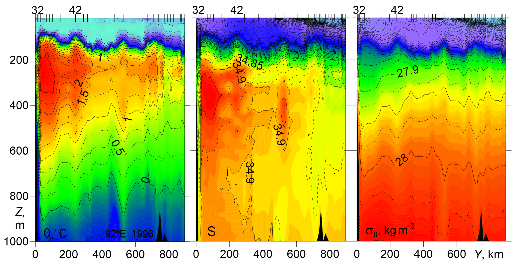
Figure 4Temperature θ, salinity S, and potential density anomaly σθ vs. distance and depth for cross-shelf transects at 92∘ E (PS96).
According to Schauer et al. (2002b), who studied the PS96 section, the horizontal and vertical scales of the BSBW were taken at 30 km and 800 m, respectively. This differs from our interpretation based on the definition of BSBW with temperature less than 0 ∘C.
Further east, in the longitude range of 94–107∘ E (NABOS09), the denser part of BSBW under the FSBW is characterized by an eastward geostrophic current with isopycnals sloping towards the north in a 150 km wide zone adjacent to the slope (see Fig. 5a–c). Less-saline water at the slope is the less dense BSBW that has entered the Nansen Basin when the slope narrows north of Severnaya Zemlya (Schauer et al., 1997).
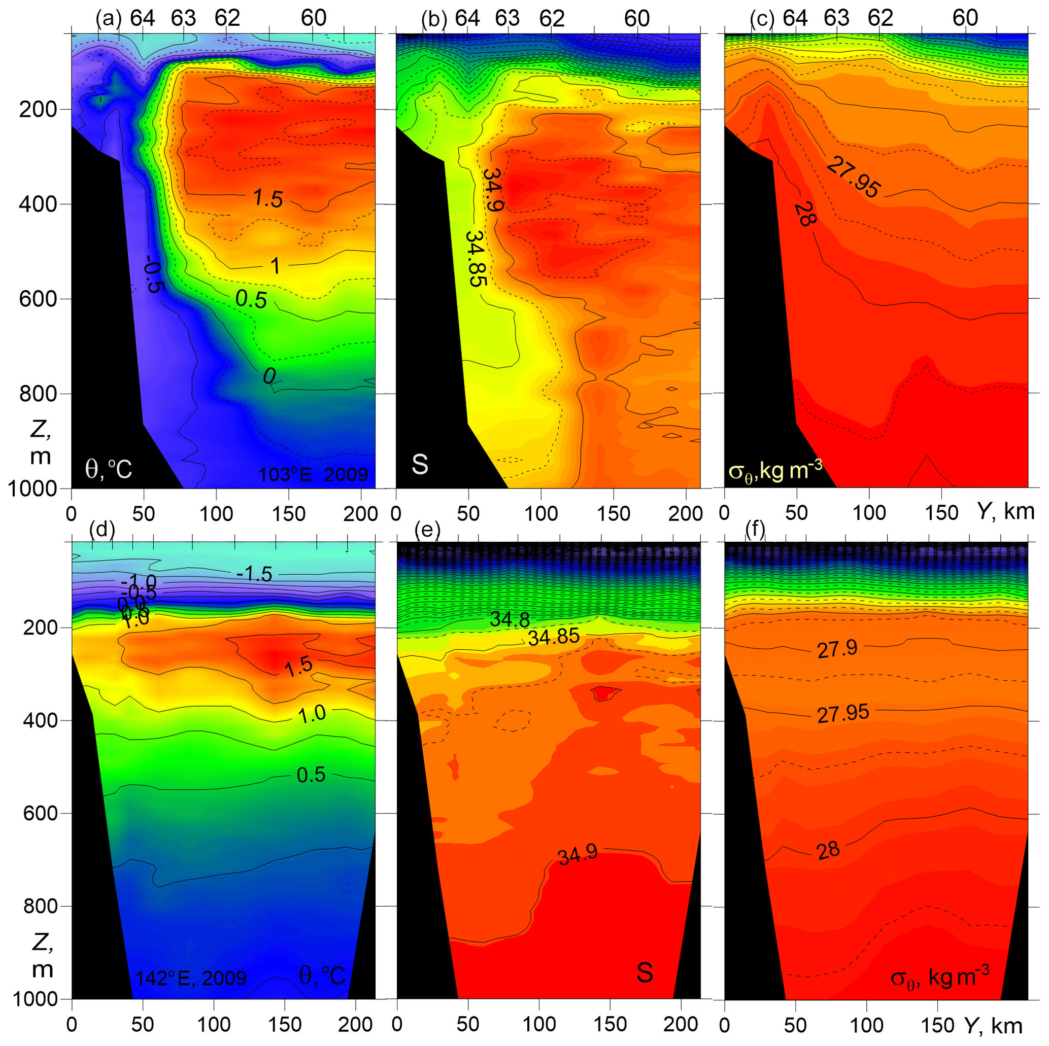
Figure 5Temperature θ, salinity S, and potential density anomaly σθ vs. distance and depth for cross-shelf transects at 103∘ E (a–c) and 142∘ E (d–f) (NABOS09).
The vertical location of the FSBW layer is similar to 92∘ E in the section PS96, but the maximum temperature has further decreased: in the transect in Fig. 5a–c, θmax=1.98 ∘C at m and Smax=34.95 at m. Figure 5d–f present the transect at 142∘ E (NABOS09) which is located on the Lomonosov Ridge, between the Amundsen and Makarov basins. The comparison of the two transects obtained in the same year shows that the vertical scale of the warm FSBW (θ>1.5 ∘C) has significantly decreased. Nevertheless, the FSBWs are also observed at this longitude and affect the slopes of isopycnic surfaces in a layer up to 300 m. The cold waters with θ<0 ∘C, which can be associated with the BSBW, are observed only at two stations in the depth range close to 1000 m and are absent at depths above 950 m. The isopycnic surfaces in Fig. 5d–f are relatively flat, indicating weak geostrophic flow (see Sect. 3.2). The “absolutely stable” thermohaline stratification below the temperature maximum with temperature decreasing and salinity increasing with depth (Fig. 5d–f) is common in the Upper Polar Deep Water (UPDW) layer (Rudels et al., 1999).
In Fig. 6 three transects are presented, at 126 and 142∘ E (NABOS05) and in the Makarov Basin at 159∘ E (NABOS07). On the transect along 126∘ E large slopes of isopycnic surfaces are observed, which corresponds to a fairly strong geostrophic flow (see Sect. 3.2), confined to the depth range of 200–400 m, that is, to the area occupied by the FSBW. At the 142∘ E transect on the Lomonosov Ridge and at the 159∘ E transect in the Makarov Basin, the FSBW can be still identified as a warm layer between 200 and 400 m, where the maximum temperature is reduced to 1.49 and 1.42 ∘C, respectively (Fig. 6). The 142∘ E transect implies some eastward geostrophic transport, whereas at the 159∘ E transect and in the area of cold waters (below 800 m) in the sections shown in Fig. 6, the baroclinic flow is weak or absent.
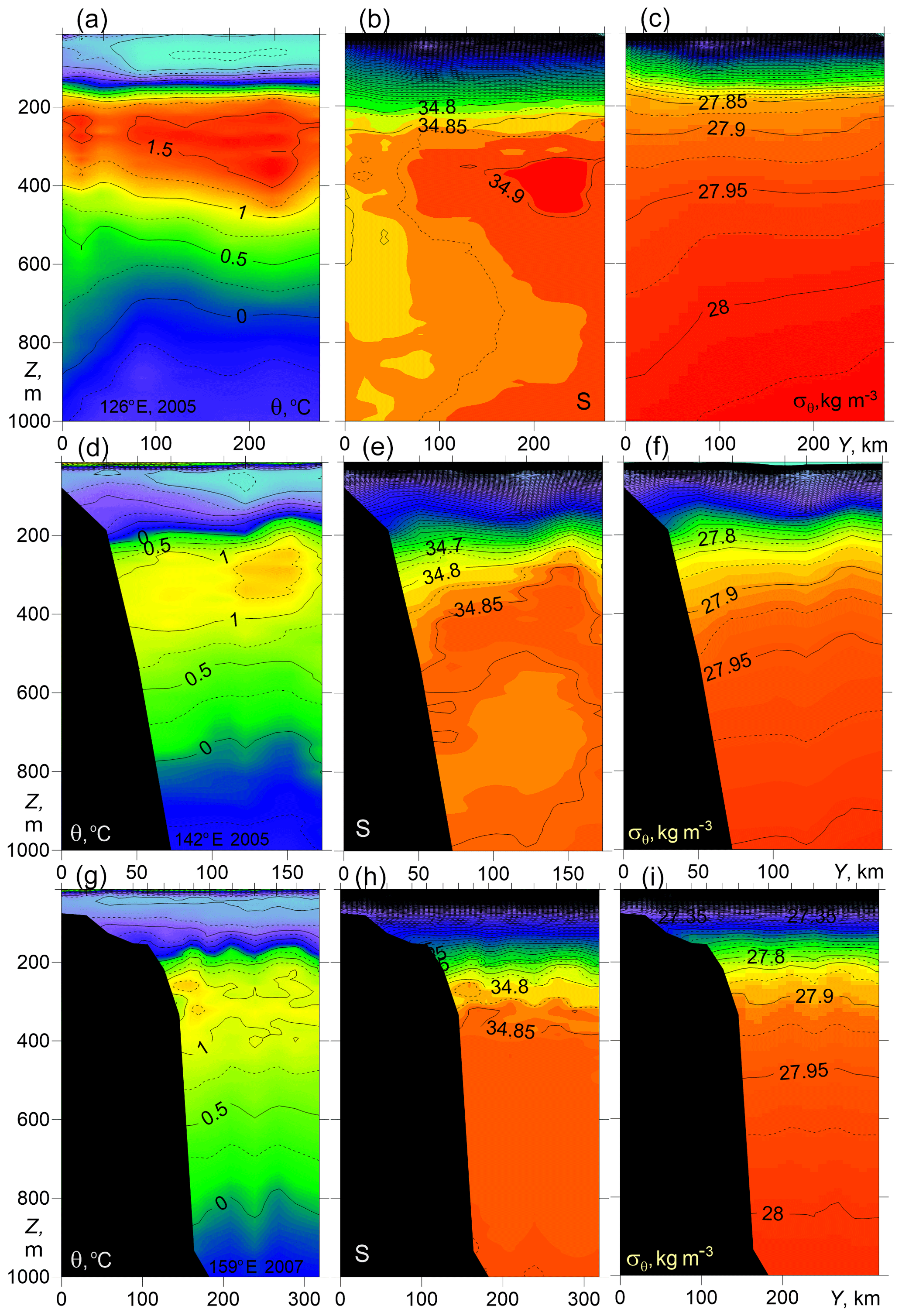
Figure 6Temperature θ, salinity S, and potential density anomaly σθ vs. distance and depth for cross-shelf transects at 126, 142∘ E (a–c and d–f, NABOS05) and 159∘ E (g–i, NABOS07).
In summary, a combined FSBW–BSBW structure with isopycnals sloping down to the north (from the slope) is typical for the longitude range 94–107∘ E. In the transects along 126, 142, and 159∘ E, sloping isopycnals were observed generally in the depth range of 200–400 m, that is in the area occupied by the FSBW. As the FSBW moved along the continental slope of the Eurasian Basin, its core temperature decreased but could be identified at all transects, including the two transects in the Makarov Basin (159∘ E). The cold waters in the transects along 126, 142, and 159∘ E, which can be associated with the BSBW, had a minimum temperature above −0.5 ∘C, were located below 800 m, and had relatively flat isopycnic surfaces.
3.1.2 θ–S analysis
The difficulty in identifying the BSBW in the eastern part of the Nansen Basin is related to the overlapping ranges of temperature and salinity inherent to the BSBW and the UPDW: , and the salinity is close to 34.9 (Rudels et al., 1994; Walsh et al., 2007). It is also important to note that the BSBW in the St. Anna Trough mixes with the FSBW. Therefore, it is not only the cold Atlantic waters, which are transported by the bottom gravity current, but also mixed warmer waters that can enter the Nansen Basin through the trough (see Fig. 3). A detailed θ–S analysis of different CTD sections can provide useful information on the transport and transformation of FSBW and BSBW. A distinct θ–S signature indicates that the water mass has entered the area of observation. The absence of a signature in the θ–S space indicates either that the water mass did not enter the area of observation or that it was transformed after mixing with other waters.
The differences in the behavior of the θ–S values are observed in the upper and deep layers of the Eurasian Basin and the St. Anna Trough (Fig. 7). On the other hand, one cannot miss a similarity in the shape of the θ–S curves in the salinity range of 34.5–35.0. The similarity is obviously caused by the presence of FSBW. Figure 7 demonstrates the transformation of the FSBW and BSBW moving along the continental slope of the Eurasian Basin. More detailed information on the BSBW transformation can be extracted from θ–S diagrams presented in Fig. 8.
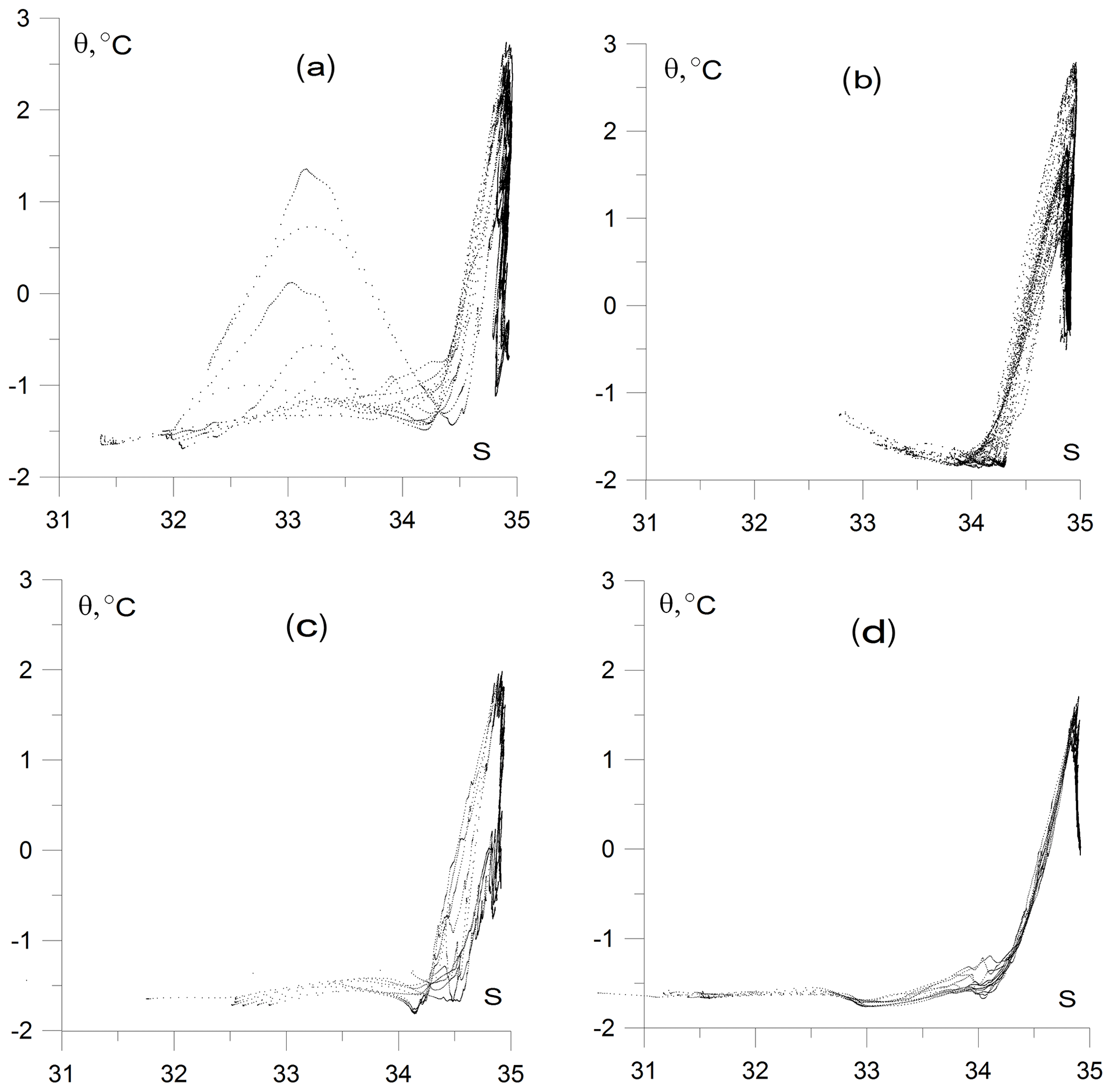
Figure 7θ–S diagrams based on the CTD profiling in (a) the St. Anna Trough (NABOS09, 82∘ N), (b) the PS96 section at 92∘ E, and the NABOS09 sections at 103∘ E (c) and 142∘ E (d). For convenience of presentation, the points of the θ–S curves with salinity below 30 were excluded.
The θ–S curves marked as 1 and 2 in Fig. 8a correspond to stations 76 and 78, respectively, which were located at the eastern slope of the St. Anna Trough just in the near-bottom gravity current carrying the BSBW, while the curves marked as 3 and 4 correspond to stations 83 and 80 located near the midpoint (thalweg) of the trough in the western periphery of the gravity current (the location of the stations is shown in Fig. 3). To visualize the BSBW transformation better, the points of θ–S curves in the temperature and salinity ranges of θ>1.2 ∘C and S<34.76, respectively, were omitted. Similar θ–S curves in the St. Anna Trough were observed within NABOS program in other years (NABOS13, NABOS15).
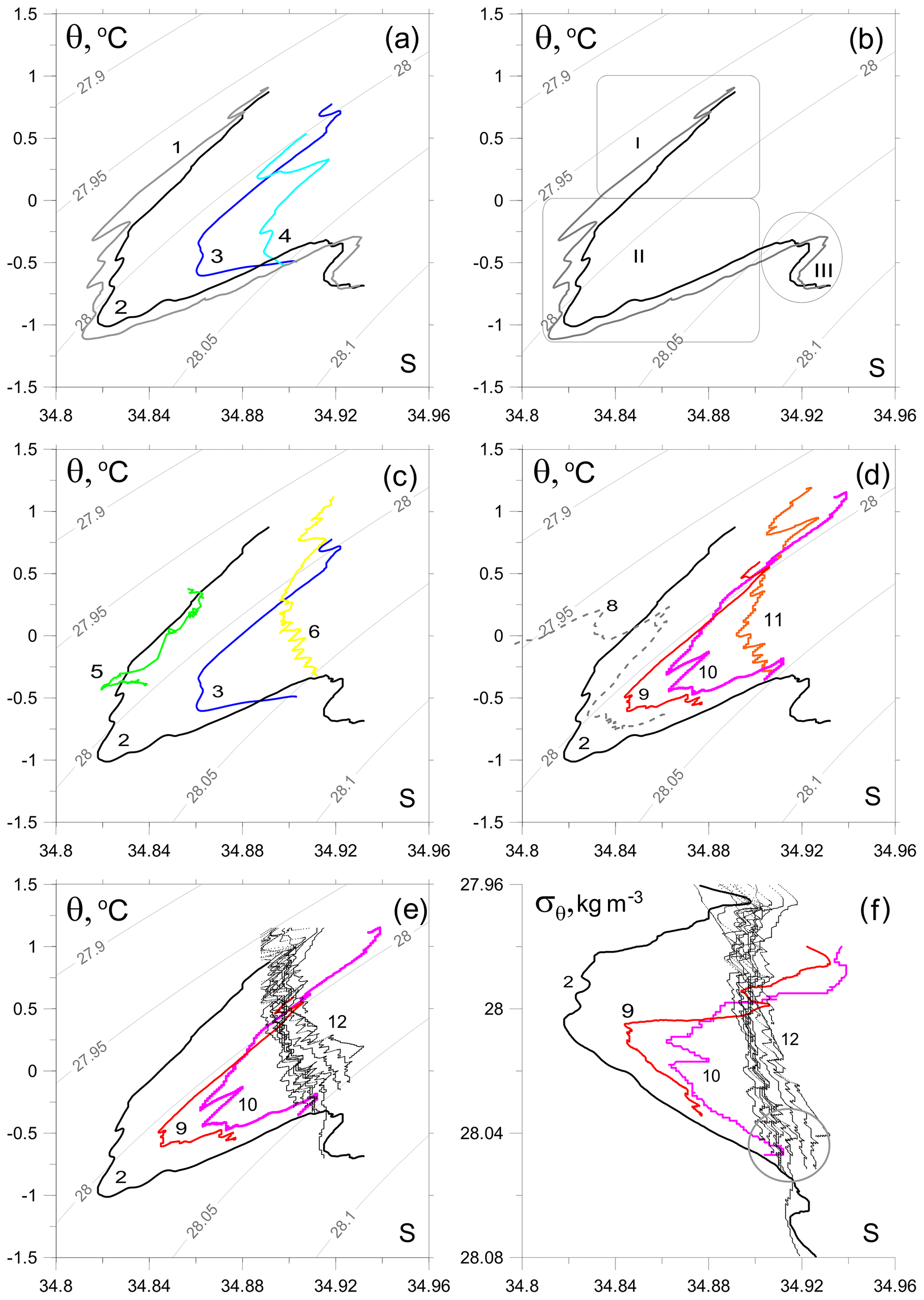
Figure 8Thermohaline values of the BSBW and FSBW. (a) Based upon the CTD profiles, obtained in the St. Anna Trough (NABOS09, section 82∘ N); curves 1–4 correspond to the stations (st.) 76, 78, 83, and 80, respectively. (b) The same as (a) but only curves 1 and 2 are presented; regions I, II, III illustrate three different water masses in accordance with Dmitrenko et al. (2015); for an explanation, see the text. (c) Based upon the section of PS96, curves 5 and 6 corresponding to st. 32 and 42, respectively (depth range 600–1000 m), curves 2 and 3 are shown for the reference. (d) For CTD profiles in the 103∘ E section, NABOS09, curve 8 (st. 64), curve 9 (st. 63), curve 10 (st. 62), curve 11 (st. 60), and curve 2 for the reference (see Fig. 5 for the location of the stations). (e) Based upon the CTD profiles in the depth range 500–1200 m measured at 126∘ E (section of NABOS09), curves 12; curves 2, 9, and 10 are shown for the reference. (f) The same as (e) but presented in coordinates σθ and S.
The curves 1 and 2 in Fig. 8a have a similar knee-like shape (Dmitrenko et al., 2015) formed by (i) the upper warm and saline water layer of the FSBW (θ≫0 ∘C), (ii) the intermediate colder and fresher water layer of BSBW (θ<0 ∘C) underlying the FSBW, and (iii) the denser, warmer and saltier “true” mode of the BSBW (θ≈ 0 ∘C); see Fig. 8b: FSBW (region I), BSBW (region II), “true” mode BSBW (region III). The BSBW differs from the “true” mode BSBW and is more diluted with the colder and fresher Barents Sea water (for more details, see Dmitrenko et al., 2015). We will be interested in the transformation of the main part of the knee (region II), namely the transformation of BSBW.
In Fig. 8c the comparison of typical θ–S curves related to the St. Anna Trough (they are also shown in the other panels of Fig. 8 for reference) with that of the 92∘ E section of PS96 is given: the curves 5 and 6 correspond to station (st.) 32 and st. 42 (depth range 600–1000 m) of the PS96 section, respectively. St. 32 was located next to the slope, while st. 42 was located about 250 km away from the slope. The coincidence of curve 5 with a part of curve 2 implies a BSBW flow along the slope of the Nansen Basin (see Fig. 4). Curve 6 corresponds to the UPDW. The θ–S diagrams for CTD profiles in the section 103∘ E are presented by curves 8–11 (see Fig. 5 for the locations of stations). Curves 8, 9, and 10 are similar to curve 2 and indicate the BSBW. Curve 11, similar to curve 6 in Fig. 8c, corresponds to the UPDW. However, the BSBW is not observed at 126∘ E: see Fig. 8e, where a collection of θ–S curves (collectively referred as 12) presents all CTD profiles in the depth range 500–1800 m measured at 126∘ E of NABOS09. Also, we do not observe the BSBW further to the east on the 142∘ E section of NABOS09 (not shown) or in the Makarov Basin.
The BSBW at 103∘ E is also characterized by a knee shape in σθ and S coordinates (Fig. 8f, numbers correspond to those in other panels). However the knee-shape diagram is not observed along 126∘ E (curves 12) in these coordinates. The dense and cold deep waters in the section 126∘ E have σθ, θ, and S values typical for the “true” BSBW mode (Dmitrenko et al., 2015). Nevertheless, these waters (see σθ and S values inside the circle; Fig. 8f) also correspond to the UPDW characteristics and hence cannot be distinguished as the “true” BSBW mode. To evaluate the transformation of the “true” mode of BSBW an additional analysis is required, which is beyond the scope of this paper.
The BSBW, which is characterized by the knee-shape diagram in coordinates θ–S and σθ–S, is not visible at 126∘ E (Fig. 8). This is consistent with the conclusion formulated in Sect. 3.1.1 that by 126∘ E the BSBW is not accompanied by any noticeable tilt of isopycnals. Moreover, given the characteristic feature of the θ–S structure of BSBW in the St. Anna Trough (curves 1–4 in Fig. 8a) was observed in other years, we carried out a similar analysis using all available CTD data and found that the BSBW is not distinct at this longitude (see Fig. 9). The only exception was 2002, when the BSBW was still observed at 126∘ E. It suggests that the BSBW and FSBW begin to mix intensively immediately after 103∘ E. On the other hand, the FSBW is well identified at 126∘ E and further along the slope of the Eurasian Basin (and even in the Makarov Basin), while we cannot say the same about the BSBW. Thus, one may assume that east of 126∘ E the geostrophic volume flow rate of the AW is mainly provided by the FSBW.

Figure 9θ–S diagrams based on the CTD profiling: NABOS05 – (a, b), 103∘ E (a), 126∘ E (b); NABOS06 – (c, d), 103∘ E (c), 126∘ E (d); NABOS08 – (e, f), 103∘ E (e), 126∘ E (f).
3.2 Characteristics of the Atlantic water flow and geostrophic estimates of the volume flow rate
The estimates of the geostrophic volume flow rate and the hydrological parameters describing the AW flow in the Eurasian and Makarov basins are presented in Table 1. The geostrophic estimates of the near-bottom volume flow rate of the BSBW in zonal transects across the St. Anna Trough are presented in Table 2. The only exception is the transect at 82∘ N, where the near-bottom gravity current with a considerable eastward component due to overflow across a sufficiently deep ridge (≈500 m deep) east of the St. Anna Trough (Fig. 3a–c) makes the estimate of AW transport northward questionable. Note also that to the west of the St. Anna Trough our estimates refer to the FSBW; to the east of this region BSBW enters the Eurasian Basin and our estimates should be attributed to the joint contribution of the two branches (FSBW and BSBW).
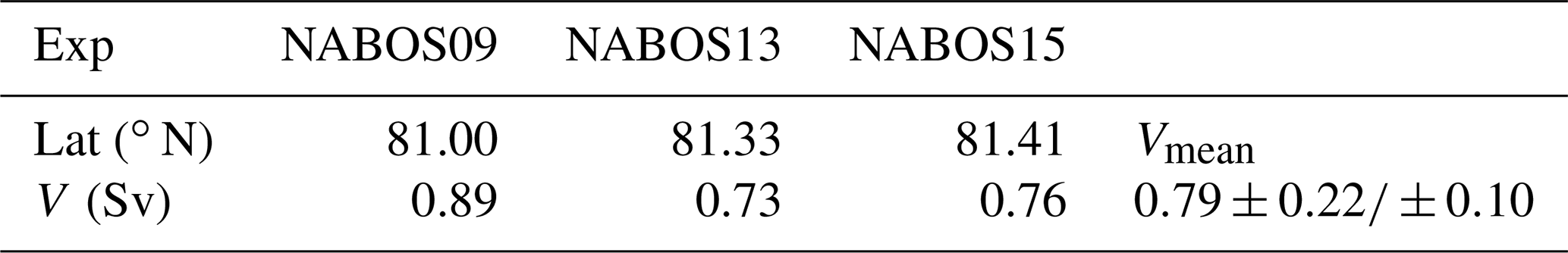
Table 1Characteristics of the Atlantic water flow in the course of its propagation along a continental slope of the Eurasian Basin of the Arctic Ocean. “Dist” is the along-slope distance from Fram Strait; θmax is the maximum temperature; , , , and are the values of potential density, salinity, depth, and lateral displacement from the slope for the point θmax; Smax and are the maximum salinity and depth of Smax; V is the geostrophic estimate of the volume flow rate. The mean values, 95 % confidence intervals, and 80 % confidence intervals of the volume flow rate, Vmean, calculated separately for CTD transects at 31–92, 94–107, 126, 142, and 159∘ E, are also shown. The last row in the Table presents the characteristics of the return flow of the AW by the Lomonosov Ridge at 140∘ E and 86.5∘ N (PS96; see Fig. 1).
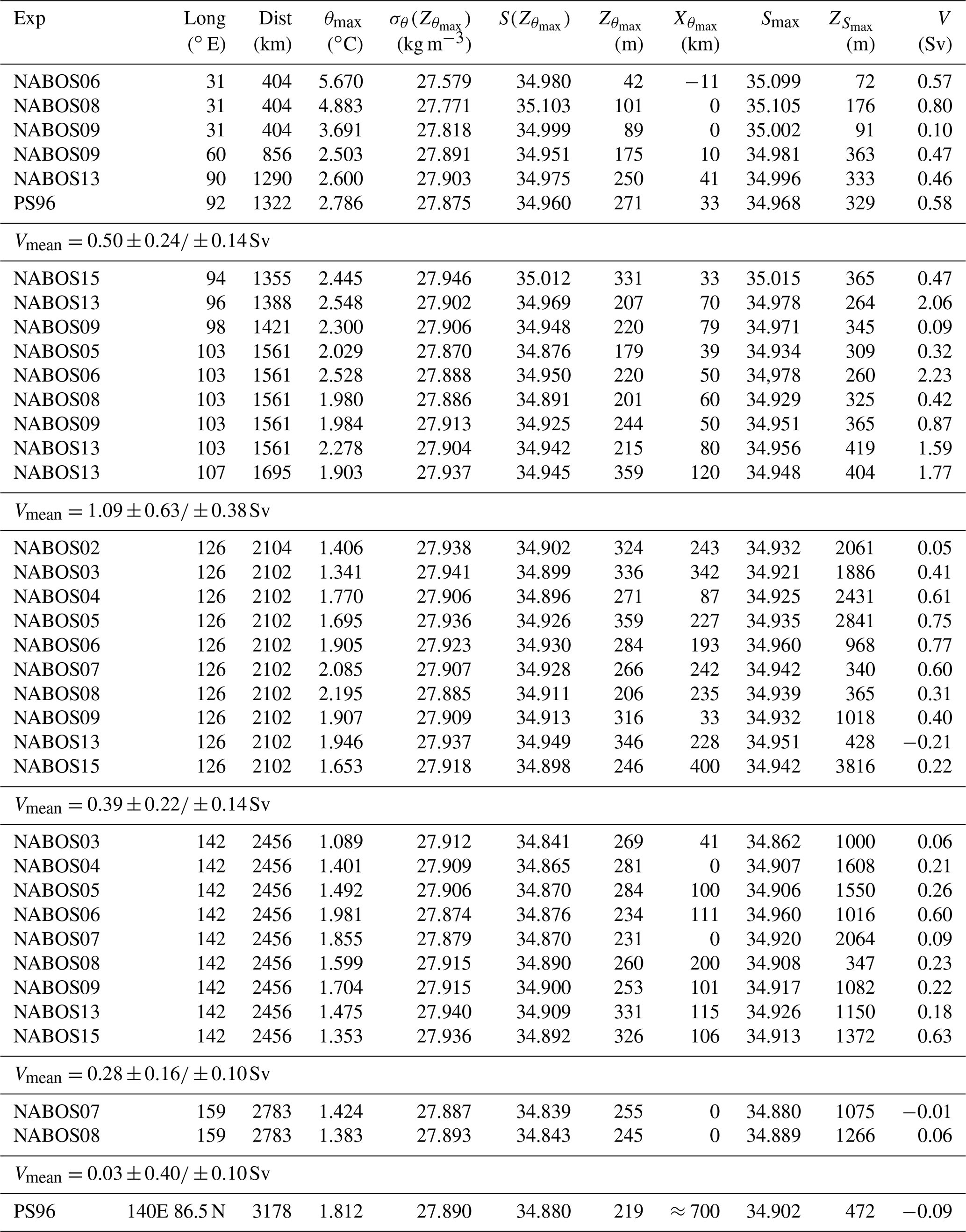
The hydrological parameters shown in Table 1 can be interpreted as follows. The maximum water temperature of the AW may exceed 5 ∘C in cases when the AW inflow to the Eurasian Basin consists of especially warm water masses. Typical changes in the temperature and salinity maxima of the AW moving along the slope over a distance of about 1000 km are approximately 1–2 ∘C and 0.1, respectively. These changes lead to a slight increase in potential density, and therefore a deviation of the AW from the isopycnic distribution can be expected. These changes are most likely associated with the exchange of heat, salt, and mass with the surrounding waters through intrusive layering and double diffusion (see, e.g., Kuzmina et al., 2011, 2018; Polyakov et al., 2012) and sea ice melting and cooling (Rudels, 1998). The intrusions, in particular, can also contribute to the reduction in the AW heat and salt content and the volume flow rate. The differences in the AW heat and salt content and the volume flow rate can be clearly seen from the PS96 section when comparing data from stations near the continental slope of the Eurasian Basin at 92∘ E and from the vicinity of the Lomonosov Ridge at 140∘ E.
Table 2Geostrophic estimates of the volume flow rate for near-bottom gravity flow of the Barents Sea branch of Atlantic water (BSBW) on zonal transects across the St. Anna Trough. The uncertainty estimates are 95 % and 80 % confidence intervals.
It is worth noting that the maximum value of the AW temperature (θmax) in this data set is always observed in the upper layer of the Eurasian Basin at depths below the pycnocline but not exceeding 350 m, while the maximum salinity (Smax) at sections in the eastern part of the basin can be observed at depths greater than 1000 m.
in Table 1 is the distance of the AW core (which can be associated with θmax) from the slope–shelf boundary. The highest value and the maximum variation in this parameter are observed near 126 and 142∘ E, where a two-core structure of AW is often observed (Pnyushkov et al., 2015).
The noticeable increase in θmax in 2006 at 31 and 103∘ E and the intensive warming of the AW were first reported in Polyakov et. al. (2011). The present results show that the increase in the temperature of the AW in 2006 was also accompanied by an increase in volume transport (see Table 1, the section along 103∘ E, and reasonings below). This can be caused not only by the warming of the AW but also by an increased inflow of the AW to the Eurasian Basin.
The geostrophic transport in the range of 31–159∘ E is characterized by a high variability (Table 1). This may be due to (a) a section orientation oblique to the current; (b) the difference in the horizontal scales of the sections; (c) uncertainty in the choice of the reference level for geostrophic calculations; (d) meandering of the flow; and (e) the effect of synoptic quasi-geostrophic eddies on the flow volume rate. In order to find statistically consistent estimates of the variability of geostrophic volume flow rate along the slope of the basin based on a limited data set, the following was done. The volume flow rates obtained for all sections within the range 31–92∘ E for different years were used to calculate the mean volume flow rate (region I; the number of volume flow rate values averaged is N=6). Similarly, the average volume flow rate was calculated for the region 94–107∘ E (region II; N=9). The remaining average estimates of geostrophic volume flow rate were calculated for sections 126∘ E (region III; N=9), 142∘ E (region IV; N=10), and 159∘ E (region V; N=2). Then the 95 % and 80 % confidence intervals were determined using the Student t distribution. All estimates of average volume flow rates and confidence intervals are presented in Tables 1 and 2.
On average, the volume flow rate increases from region I to region II and then decreases to region III and region IV, followed by a sharp decrease in region V. However, only the difference between the volume flow rate in region II and the values in regions IV and V are significant at 95 % confidence. Transport values bounded by the confidence intervals for regions II, IV, and V are (0.46; 1.72), (0.12; 0.44), and (−0.37; 0.43), respectively. These intervals indicate that the mean volume flow rate in region II exceeds the value of the same parameter in regions IV and V with a high probability of 95 %. The 80 % confidence intervals overlap only for regions III and IV: (0.25; 0.53) and (0.18; 0.38), respectively. In this regard, the change in the volume flow rate along the slope is significant with a probability of 80 %, except for changes in volume flow rate from region III to region IV.
The above values of the mean volume flow rate and confidence intervals also suggest that the increase in volume flow rate in 2006 is significant and not caused by the “noise” in the data. Indeed, the volume flow rates in regions II, III, and IV in 2006 exceeded the upper limits of the corresponding 95 % confidence intervals. From a statistical point of view such a significant increase in volume flow rates at the same time in three regions is a very rare event that can hardly be explained by random “noise” in the data caused, for example, by the influence of synoptic eddies.
Let us turn our attention to the following features of the volume flow rate estimates: high volume flow rate estimates at 96, 103, and 107∘ E, a negative volume flow rate estimate at 126∘ E in 2013, and low volume flow rate estimates at 31 and 98∘ E in 2009 (Table 1). Indeed, the AW volume flow rate in the BSBW area of entry into the Eurasian Basin in 2013 was almost equal to the maximum volume flow rate in 2006 (103∘ E) and was quite high, up to the longitude 107∘ E. This phenomenon as well as the intense warming in 2006 can be associated with the recent changing conditions in the Arctic. We hypothesize that the negative volume flow rate at 126∘ E was because of the influence of local return flows which can be observed near the slope (Pnyushkov et al., 2015). Low FSBW volume flow rate estimates in 2009 are probably associated with a strong deviation of the flow from the slope, which may underestimate the AW volume transport due to the small length of the transects to the north (see also Sect. 4).
The mean value of the FSBW volume flow rate in region I is Vmean=0.5 Sv. This estimate of volume flow rate is about half the estimate of the BSBW mean volume flow rate: Vmean=0.79 Sv (N=3, Table 2). (The difference is significant at 80 % confidence interval.) The BSBW mean volume flow rate exceeding nearly twice the FSBW mean volume flow rate results in a dominance of the BSBW pattern of potential density contours in the longitude range of 94–107∘ E (region II), where both branches of the AW are present. Moreover, the sum of the mean values of the FSBW and the BSBW geostrophic volume flow rate estimates Sv corresponds well to the combined FSBW and BSBW flow within the region II: Vmean=1.09 Sv. Thus, the increase in geostrophic volume transport in region II is mainly due to the influence of the BSBW. The decrease in geostrophic volume transport in region III can also be associated primarily with the BSBW, namely, with the decrease in the BSBW volume transport in the 126∘ E section and further along the slope (see Sect. 3.1.1 and 3.1.2).
Finally, at the 159∘ E section in the Makarov Basin, the geostrophic estimate of the along-slope volume flow rate of mixed waters of the FSBW and the BSBW has further greatly reduced down to Vmean=0.03 Sv (N=2), which is more than 1 order of magnitude smaller than that in the Nansen and Amundsen basins. Despite the low statistical significance of the latter estimate (due to the small value of N=2) one may conclude that the major part of the AW entering the Arctic Ocean circulates cyclonically within the Nansen and Amundsen basins, and only its small part flows to the Makarov Basin (Rudels et al., 2015; Rudels, 2015). However, additional studies are required to confirm this result.
3.3 Interannual variability of the AW temperature–salinity values and the volume flow rate
Within the NABOS project, the cross-slope CTD transects at 103, 126, and 142∘ E were repeatedly performed for a number of annual campaigns (Table 1): 2005, 2006, 2008, and 2013 (103∘ E); 2002–2009, 2013, and 2015 (126∘ E); 2003–2009, 2013, and 2015 (142∘ E). We use the repeated transects to describe the interannual variability of the AW.
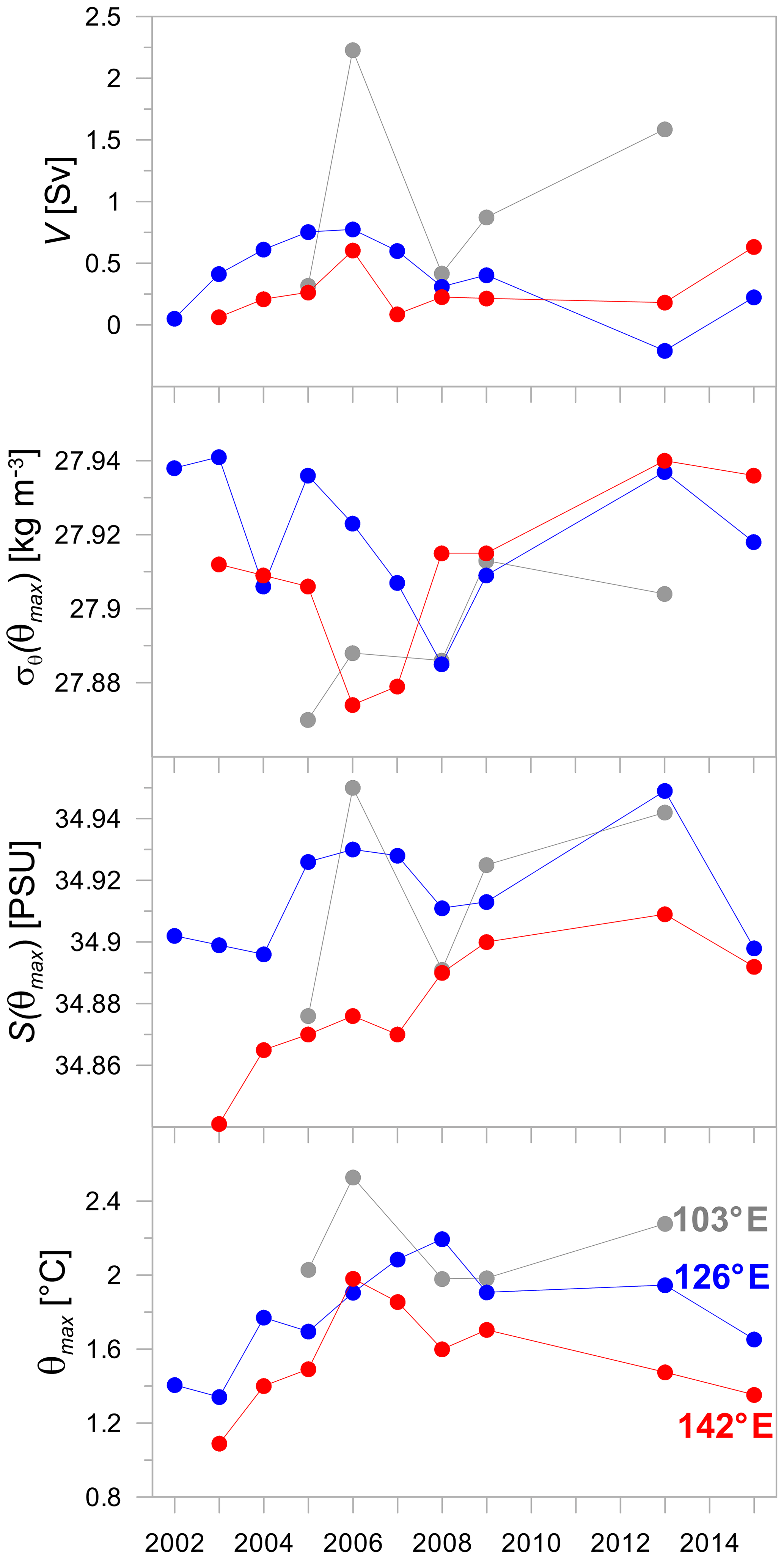
Figure 10Interannual variability of the maximum temperature θmax and the related values of salinity S(θmax), potential density anomaly σθ(θmax), and volume flow rate V on the cross-slope transects at 103, 126, and 142∘ E.
Time series of the AW temperature maximum, θmax, and the related values of salinity S(θmax) and potential density anomaly σθ(θmax) (Fig. 10) show that the period of 2006 to 2008 was characterized by an increased temperature of the AW in the eastern part of the Eurasian Basin, an increased salinity and density reduction. The temperature excess during this period was as large as 0.6–1.0 ∘C relative to 2002–2003 and 0.3–0.6 ∘C relative to 2013–2015. In 2006, S(θmax) displayed local maxima at the transects 126 and 142∘ E and the absolute maximum at the transect 103∘ E; the salinity excess for the maxima largely decreased with the longitude from approximately 0.06 at 103∘ E to less than 0.01 at 142∘ E. θmax had a maximum in 2013 but only at 103∘ E (see Table 1 and Fig. 10). The time series of S(θmax) display a trend of increase in AW salinity over time, which can be referred to as an AW salinization in the early 2000s. The salinity of AW at 142∘ E increases almost monotonously in the period from 2003 to 2013. The mechanism behind this salinity evolution is not clear. It is also worth noting that the maxima of θmax and S(θmax) in 2006 and 2013 (at 103∘ E) were accompanied by maxima in transport.
Here we discuss the following issues: (a) differences in the identification of the BSBW; (b) a comparison of the geostrophic volume flow rate estimates with other studies; (c) the weakening of the BSBW signal at 126∘ E and further east.
- a.
Advection and interaction of waters with different θ–S characteristics in the Arctic Basin, as well as the impact of climate change that has been observed over the past decade (Polyakov et al., 2017) complicate an accurate identification of water masses. However, a robust approach proposed in Dmitrenko et al. (2015) is effective for distinguishing the water masses of the FSBW and BSBW branches. As an exception, this approach fails when the FSBW temperature is below 0 ∘C (see Fig. 2 in Dmitrenko et al., 2015) and/or the BSBW temperature is close to 1 ∘C (see Fig. 6 in Schauer et al., 2002a). If such cases are rare, then either of the two approaches can be used to identify the BSBW and FSBW. Indeed, the identification of the BSBW on the PS96 section in our case (we used the approach proposed by Dmitrenko et al., 2015; see Sect. 3.1.1) does not differ much from that proposed by Schauer et al. (2002b). However, these discrepancies can lead to almost an order of magnitude difference in estimates of the volume flow rate of the BSBW only due to the differences in the BSBW cross-sectional area.
- b.
Based on the velocity measurements with moored instruments (1997–2010) in the area of the West Spitsbergen Current (WSC) near Fram Strait (zonal transect at ∼78∘50′ N) , approximately 3 Sv of the AW flows into the Nansen Basin (Beszczynska-Möller et. al., 2012). The long-term mean volume transport confined to the WSC core branch (or Svalbard branch in accordance with Schauer et al., 2004) included 1.3±0.1 Sv of the AW warmer than 2 ∘C. The offshore WSC branch (or Yermak branch) carried on average 1.7±0.1 Sv of the AW. The variability range of the AW geostrophic transport of the Svalbard branch for meridional sections from 1997, 2001, and 2003 (summer and fall) was between 0.06 and 0.7 Sv (Marnela et al., 2013). In Kolås and Fer (2018) observations of the oceanic current and thermohaline field (in summer 2015) in the three sections were used to characterize the evolution of the WSC along 170 km downstream distance. Absolute geostrophic transports of AW ranged from 0.6 to 1.3 Sv in the Svalbard branch. In accordance with earlier studies of the currents in Fram Strait, recirculation of the AW can be significant, and the volume flow rate of the AW entering the Arctic Ocean ranges from 0.6 to 1.5 Sv (Rudels, 1987; Aagaard and Carmack, 1989).
Our estimate of the mean volume flow rate Vmean in region I (31–92∘ E) is in the range of the above estimates. However, the upper confidence limit of our estimate does not reach 1 Sv. Moreover, we used T>0 ∘C to identify the AW, while in Beszczynska-Möller et al. (2012) the volume flow rates of the AW entering the Eurasian Basin through Fram Strait were determined for waters with T>2 ∘C. Comparatively smaller transport in region I may be because the sections along 31∘ E (see Fig. 1) are less than 100 km wide and do not cover the full extent of the FSBW (Fig. 2). Given the sensitivity to the definition of AW and the resulting cross-sectional area (see point “a” above), the volume transport may be underestimated. It is possible that the formation and passage of synoptic eddies leads to variability in volume transports. According to Perez-Hernandez et al. (2017) north of Svalbard (between 21 and 33∘ E) in September 2013, a large difference was found in the estimates of geostrophic volume flow rate (from 0.53 to 3.39 Sv) due to the passage of eddies and meandering of the current. Våge et al. (2016) based on geostrophic velocities at two CTD sections across the boundary current near 30∘ E (September 2012) evaluated a net AW volume flow rate of 1.6±0.3 Sv. They found evidence of a large eddy affecting the mean volume transport calculations. The barotropic velocity component, which is not taken into account in our estimates, can also contribute to larger transports. However, in conditions with high ice concentration in the Eurasian Basin, we might expect a reduced barotropic contribution from the sea level changes induced by wind forcing. In cruise reports, the NABOS CTD sections were characterized by ice concentrations of 50 %–100 % (see https://uaf-iarc.org/nabos-cruises/, last access: 3 May 2019, IARC, 2019). Exceptions occurred in the near-slope areas of the Laptev Sea, that is, in the sections along ∼126∘ E, where the ice concentration varied from 0 % to 100 %, having a maximum value in the northern part of the sections. In such areas, the contribution of the barotropic component to the flow velocity can be large. For example, using long-term measurements (1995–1996) from a mooring in the near-slope area of the Laptev Sea, Woodgate et al. (2001) showed that the contribution of the barotropic component to the velocity of the Arctic Ocean boundary current (AOBC) was equal to the contribution of the first three baroclinic modes. Assuming an average velocity based on the measurements in the upper 1200 m layer of 4.5 cm s−1 and a width of 50 to 84 km the volume flow rate was estimated at 5±1 Sv. This is larger than our average estimate of the AW volume flow rate along 126∘ E (0.39±0.22, Table 1) by an order of magnitude. Such a difference can be explained not only by the absence of a barotropic contribution in our case, but also by the fact that we took into account the volume transport of AW only (i.e., the cold, low-salinity surface layer was excluded) and considered a certain season (August and September). Indeed, according to long-term measurements at six moorings on a section along 126∘ E, the AOBC volume flow rate varied from 0.3 to 9 Sv (Pnyushkov et al., 2018b). Such a wide range in volume flow rate estimates is probably due to a combined effect of seasonal variability and mesoscale eddies (Pnyushkov et al., 2018a).
The fact that seasonal variations can in some cases significantly affect the AW volume flow rates (see also the discussion in Pnyushkov et al., 2018b) is confirmed by a number of observations (Schauer et al., 2002a; Beszczynska-Möller et al., 2012; Pnyushkov et al., 2018b). For example, the volume flow rate of the AW in the northwestern part of the Barents Sea was 0.6 Sv (Schauer et al., 2002a). This agrees well with our estimate of the AW transport in the St. Anna Trough of 0.79±0.22 Sv (Table 2). However, the analysis of current velocity measurements in the winter season at the same section in the northwestern part of the Barents Sea gave a completely different estimate of ∼2.6 Sv (Schauer et al., 2002a).
- c.
According to Dmitrenko et al. (2009), the BSBW can be satisfactorily identified at 142∘ E. However, a “pattern” in the θ–S diagram far from the place of the BSBW entry into the Eurasian Basin can be regarded as the BSBW signal if it maintains the similarity with the “pattern” of the BSBW at the exit from the St. Anna Trough, that is, with the so-called “knee” (Dmitrenko et al., 2015). Our analysis showed that the “knee” is regularly observed at 103∘ E, while at 126∘ E it is absent, weak, or distorted. This may be expected since the flow velocity is small and the BSBW covers a distance from 103 to 126∘ E for 1–2 years. However, despite such a long travel time, Fram Strait branch is well identified not only at 126∘ E but also further along the slope. This suggests stronger transformation and mixing of, primarily, the BSBW. The BSBW transformation can be due to various reasons, including mixing with the FSBW caused by thermohaline intrusive layering at absolutely stable stratification (Merryfield, 2002; Kuzmina et al., 2014; Kuzmina, 2016), the influence of the slope topography, the impact of local counterflows near the slope (see, for example, Pnyushkov et al., 2015), lateral convection (Ivanov and Shapiro, 2005; Ivanov and Golovin, 2007; Walsh et al., 2007), the impact of the Arctic Shelf Break Water (Aksenov et al., 2011; Ivanov and Aksenov, 2013), and mixing due to eddies (Schauer et al., 2002; Dmitrenko et al., 2008; Aagaard et al., 2008; Pnyushkov et al., 2018a). The understanding of the processes of transformation and mixing of the BSBW and FSBW is necessary to verify an important concept proposed by Rudels et al. (2015) that the BSBW supplies the major part of the AW to the Amundsen, Makarov, and Canadian basins, while the FSBW remains almost fully in the Nansen Basin.
The θ–S properties and the volume flow rate estimates of the current carrying the AW in the Eurasian Basin and St. Anna Trough were obtained based on the analysis of CTD data collected within the NABOS program in 2002–2015; additionally CTD transect PS96 was considered.
FSBW was present at all transects, including the two transects in the Makarov Basin (159∘ E), while the cold waters at the transects along longitudes 126, 142, and 159∘ E, which can be associated with the influence of the BSBW, were observed in the depth range below 800 m and had little effect on the spatial structure of isopycnic surfaces and the horizontal gradient of density. It is shown using θ—S analysis that the BSBW signal, which is characterized by the knee-shape feature in coordinates θ and S and σθ and S (see Fig. 8), is either strongly weakened or not visible at the longitude 126∘ E (excluding the observations in 2002 at 126∘ E), while the FSBW signal is well identified at 126∘ E and further along the slope of the Eurasian Basin. Based on the revealed features of the temperature, salinity, and density fields, it is suggested that east of 126∘ E the geostrophic volume transport of AW is mainly provided by the FSBW.
The geostrophic volume transport of AW increases (with 80 % confidence) from the region of 31–92∘ E (0.5±0.14 Sv) to the region of 94–107∘ E (1.09±0.38 Sv) and then decreases to the region of 126∘ E (0.39±0.14 Sv) and becomes small (0.03±0.1 Sv) in the Makarov Basin (159∘ E).
The temporal variability of hydrological parameters and of the AW volume flow rate is summarized as follows. The time series of θmax had an absolute maximum in 2006–2008 that can be interpreted as a result of heat pulse in the early 2000s (Polyakov et al., 2011). In accordance with our analysis the time series of θmax had a maximum in 2013 but only at the longitude 103∘ E (Table 1 and Fig. 10). The time series of S(θmax) display a trend of increase in AW salinity over time, which can be referred to as an AW salinization in the early 2000s. Moreover the salinity increases almost monotonously in the period from 2003 to 2013 at 142∘ E. It is important to underline also that the maxima of θmax and S(θmax) in 2006 and 2013 (103∘ E) are accompanied by the volume flow rate highs. A significant increase in geostrophic volume flow rate identified in 2006 is likely associated with the recent change observed in the Arctic Ocean.
All CTD data used in this paper can be accessed from the NABOS project website http://nabos.iarc.uaf.edu (last access: 24 January 2019, IARC, 2019).
NZ proposed the idea of research, developed approaches to data processing, estimated the transports and average thermohaline characteristics of Atlantic waters, and described results. NK carried out θ–S analysis and statistical analysis. Both authors contributed to the interpretation of the results and writing the paper.
The authors declare that they have no conflict of interest.
This research, including the approach development, data processing, and interpretation, performed by Nataliya Zhurbas, was funded by Russian Science Foundation (project no. 17-77-10080). Natalia Kuzmina (θ–S analysis, statistical analysis, participation in discussion) was supported by the state assignment of the Shirshov Institute of Oceanology RAS (theme no. 0149-2019-0003).
The authors are very grateful to the NABOS group for providing the opportunity to use the CTD data.
The authors are very grateful to the editor for evaluating the article and help in the work on the text and to the anonymous reviewers for useful comments.
This research was funded by Russian Science Foundation (project no. 17-77-10080) and by the state assignment of the Shirshov Institute of Oceanology RAS (theme no. 0149-2019-0003).
This paper was edited by Ilker Fer and reviewed by two anonymous referees.
Aagaard, K.: On the deep circulation of the Arctic Ocean, Deep-Sea Res., 28, 251–268, 1981.
Aagaard, K. and Carmack, E. C.: The role of sea ice and other fresh water in the Arctic circulation, J. Geophys. Res., 94, 14485–14498, https://doi.org/10.1029/JC094iC10p14485, 1989.
Aagaard, K., Andersen, R., Swift, J., and Johnson, J.: A large eddy in the central Arctic Ocean, Geophys. Res. Lett., 35, L09601, https://doi.org/10.1029/2008GL033461, 2008.
Aksenov, Y., Ivanov, V. V., Nurser, A. J. G., Bacon, S., Polyakov, I. V., Coward, A. C., Naveira-Garabato, A. C., and Beszczynska-Moeller, A.: The Arctic Circumpolar Boundary Current, J. Geophys. Res., 116, C09017, 1–28, https://doi.org/10.1029/2010JC006637, 2011.
Beszczynska-Möller, A., Fahrbach, E., Schauer, U., and Hansen, E.: Variability in Atlantic water temperature and transport at the entrance to the Arctic Ocean, 1997–2010, ICES J. Mar. Sci., 69, 852–863, https://doi.org/10.1093/icesjms/fss056, 2012.
Dmitrenko, I. A., Kirillov, S. A., Ivanov, V. I., and Woodgate, R.: Mesoscale Atlantic water eddy off the Laptev Sea continental slope carries the signature of upstream interaction, J. Geophys. Res., 113, C07005, https://doi.org/10.1029/2007JC004491, 2008.
Dmitrenko, I. A., Kirillov, S. A., Ivanov, V. V., Woodgate, R. A., Polyakov, I. V., Koldunov, N., Fortier, L., Lalande, C., Kaleschke, L., Bauch, D., Hölemann, J. A., and Timokhov, L. A.: Seasonal modification of the Arctic Ocean intermediate water layer off the eastern Laptev Sea continental shelf break, J. Geophys. Res.-Oceans, 114, C06010, https://doi.org/10.1029/2008JC005229, 2009.
Dmitrenko, I. A., Rudels, B., Kirillov, S. A., Aksenov, Y. O., Lien V. S., Ivanov, V. V., Schauer, U., Polyakov, I. V., Coward, A., and Barber, D. J.: Atlantic Water flow into the Arctic Ocean through the St. Anna Trough in the northern Kara Sea, J. Geophys. Res.-Oceans, 120, 5158–5178, https://doi.org/10.1002/2015JC010804, 2015.
IARC: Nansen and Amundsen Basins Observational System NABOS, available at: http://nabos.iarc.uaf.edu, last access: 24 January 2019.
Ivanov, V. and Golovin, P.: Observations and modelling of dense water cascading from northwestern Laptev Sea shelf, J. Geophys. Res., 112, C09003, https://doi.org/10.1029/2006JC003882, 2007.
Ivanov, V. V. and Aksenov, E. O.: Atlantic Water transformation in the Eastern Nansen Basin: observations and modelling, Arct. Antarct. Res., 1, 72–87, 2013 (in Russian).
Ivanov, V. V. and Shapiro, G. I.: Formation of dense water cascade in the marginal ice zone in the Barents Sea, Deep-Sea Res. Pt. I, 52, 1699–1717, https://doi.org/10.1016/j.dsr.2005.04.004, 2005.
Kolås, E. and Fer, I.: Hydrography, transport and mixing of the West Spitsbergen Current: the Svalbard Branch in summer 2015, Ocean Sci., 14, 1603–1618, https://doi.org/10.5194/os-14-1603-2018, 2018.
Kuzmina, N.: Generation of large-scale intrusions at baroclinic fronts: an analytical consideration with a reference to the Arctic Ocean, Ocean Sci., 12, 1269–1277, https://doi.org/10.5194/os-12-1269-2016, 2016.
Kuzmina, N., Rudels, B., Zhurbas, V., and Stipa, T.: On the structure and dynamical features of intrusive layering in the Eurasian Basin in the Arctic Ocean, J. Geophys. Res., 116, C00D11, https://doi.org/10.1029/2010JC006920, 2011.
Kuzmina, N. P., Zhurbas, N. V., Emelianov, M. V., and Pyzhevich, M. L.: Application of interleaving Models for the Description of intrusive Layering at the Fronts of Deep Polar Water in the Eurasian Basin (Arctic), Oceanology, 54, 557–566, https://doi.org/10.1134/S0001437014050105, 2014.
Kuzmina, N. P., Skorokhodov, S. L., Zhurbas, N. V., and Lyzhkov, D. A.: On instability of geostrophic current with linear vertical shear at length scales of interleaving, Izv. Atmos. Ocean. Phys., 54, 47–55, https://doi.org/10.1134/S0001433818010097, 2018.
Marnela, M., Rudels, B., Houssais, M.-N., Beszczynska-Möller, A., and Eriksson, P. B.: Recirculation in the Fram Strait and transports of water in and north of the Fram Strait derived from CTD data, Ocean Sci., 9, 499–519, https://doi.org/10.5194/os-9-499-2013, 2013.
Merryfield, W. J.: Intrusions in Double-Diffusively Stable Arctic Waters: Evidence for Differential mixing?, J. Phys. Oceanogr., 32, 1452–1459, 2002.
Pérez-Hernández, M. D., Pickart, R. S., Pavlov, V., Våge, K., Ingvaldsen, R., Sundfjord, A., Renner, A. H. H., Torres, D. J., and Erofeeva, S. Y.: The Atlantic Water boundary current north of Svalbard in late summer, J. Geophys. Res.-Oceans, 122, 2269–2290, https://doi.org/10.1002/2016JC012486, 2017.
Pfirman, S. L., Bauch, D., and Gammelsrød, T.: The northern Barents Sea: water mass distribution and modification, in: The Polar Oceans and Their Role in Shaping the Global Environment, Geophysical Monograph 85, edited by: Johannessen, O. M., Muench, R. D., and Overland, J. E., American Geophysical Union, Hoboken, NJ, 77–94, 1994.
Pnyushkov, A. V., Polyakov, I. V., Ivanov, V. V., Aksenov, Ye, Coward, A. C., Janout, M., and Rabe, B.: Structure and variability of the boundary current in the Eurasian Basin of the Arctic Ocean, Deep-Sea Res. Pt. I, 101, 80–97, https://doi.org/10.1016/j.dsr.2015.03.001, 2015.
Pnyushkov, A. V., Polyakov, I. V., Padman, L., and Nguyen, A. T.: Structure and dynamics of mesoscale eddies over the Laptev Sea continental slope in the Arctic Ocean, Ocean Sci., 14, 1329–1347, https://doi.org/10.5194/os-14-1329-2018, 2018a.
Pnyushkov, A. V., Polyakov, I. V., Rember, R., Ivanov, V. V., Alkire, M. B., Ashik, I. M., Baumann, T. M., Alekseev, G. V., and Sundfjord, A.: Heat, salt, and volume transports in the eastern Eurasian Basin of the Arctic Ocean from 2 years of mooring observations, Ocean Sci., 14, 1349–1371, https://doi.org/10.5194/os-14-1349-2018, 2018b.
Polyakov, I., Timokhov, L., Dmitrenko, I., Ivanov, V., Simmons, H., Beszczynska-Möller, A., Dickson, R., Fahrbach, E., Fortier, L., Gascard, J.-C., Hölemann, J., Holliday., N. P., Hansen, E., Mauritzen, C., Piechura, J., Pickart, R., Schauer, U., Walczowski, W, and Steele, M.: Observational program tracks Arctic Ocean transition to a warmer state, EOS T. Am. Geophys. Un, 88, 398–399, https://doi.org/10.1029/2007EO400002, 2007.
Polyakov, I. V., Alexeev, V. A., Ashik, I. M., Bacon, S., Beszczynska-Möller, A., Carmack, E. C., Dmitrenko, I. A., Fortier, L., Gascard, J.-C., Hansen, E., Hölemann, J., Ivanov, V. V., Kikuchi, T., Kirillov, S., Lenn, Y.-D., McLaughlin, F. A., Piechura, J., Repina, I., Timokhov, L. A., Walczowski, W., and Woodgate, R.: Fate of Early 2000s Arctic Warm Water Pulse, B. Am. Meteorol. Soc., 92, 561–566, https://doi.org/10.1175/2010BAMS2921.1, 2011.
Polyakov, I. V., Pnyushkov, A., Rember, R., Ivanov, V., Lenn, Y-D., Padman, L., and Carmack, E. C.: Mooring-based observations of the double-diffusive staircases over the Laptev Sea, J. Phys. Oceanogr., 42, 95–109, 2012.
Polyakov, I. V., Pnyushkov, A. V., Alkire, M. B., Ashik, I. M., Baumann, T. M., Carmack, E. C., Goszczko, I., Guthrie, J., Ivanov, V. V., Kanzow, T., Krishfield, R., Kwok, R., Sundfjord, A., Morison, J., Rember, R., and Yulin, A.: Greater role for Atlantic inflows on sea-ice loss in the Eurasian Basin of the Arctic Ocean, Science, 356, 285–291, https://doi.org/10.1126/science.aai8204, 2017.
Rudels, B.: On the mass balance of the polar ocean, with special emphasis on the Fram Strait, Skr. Nor. Polarinst., 188, 1–53, 1987.
Rudels, B.: Aspects of Arctic oceanography, in Physics of ice-covered seas, vol. 2, edited by: Leppäranta, M., Univ. Press, Helsinki, 517–568, 1998.
Rudels, B.: Arctic Ocean circulation, processes and water masses: A description of observations and ideas with focus on the period prior to the International Polar Year 2007–2009, Prog. Oceanogr., 132, 22–67, https://doi.org/10.1016/j.pocean.2013.11.006, 2015.
Rudels, B., Jones, E. P., Anderson, L. G., and Kattner, G.: On the intermediate depth waters of the Arctic Ocean, in: The Role of the Polar Oceans in Shaping the Global Climate, edited by: Johannessen, O. M., Muench, R. D., and Overland, J. E., American Geophysical Union, Washington, DC, 33–46, 1994.
Rudels, B., Björk, G., Muench, R. D, and Schauer, U.: Double-diffusive layering in the Eurasian Basin of the Arctic Ocean, J. Marine Syst., 21, 3–27, 1999.
Rudels, B., Jones, E. P., Schauer, U., and Eriksson, P.: Atlantic sources of the Arctic Ocean surface and halocline water, Polar Res., 23, 181–208, https://doi.org/10.1111/j.1751-8369.2004.tb00007.x, 2004.
Rudels, B., Korhonen, M., Schauer, U., Pisarev, S., Rabe, B., and Wisotzki A.: Circulation and transformation of Atlantic water in the Eurasian Basin and the contribution of the Fram Strait inflow branch to the Arctic Ocean heat budget, Prog. Oceanogr., 132, 128–152, https://doi.org/10.1016/j.pocean.2014.04.003, 2015.
Schauer, U., Muench, R. D., Rudels, B., and Timokhov, L.: Impact of eastern Arctic shelf waters on the Nansen Basin intermediate layers, J. Geophys. Res., 102, 3371–3382, 1997.
Schauer, U., Loeng, H., Rudels, B., Ozhigin, V. K., and Dieck, W.: Atlantic Water flow through the Barents and Kara Seas, Deep-Sea Res. Pt. I, 49, 2281–2298, https://doi.org/10.1016/S0967-0637(02)00125-5, 2002a.
Schauer, U., Rudels, B., Jones, E. P., Anderson, L. G., Muench, R. D., Björk, G., Swift, J. H., Ivanov, V., and Larsson, A.-M.: Confluence and redistribution of Atlantic water in the Nansen, Amundsen and Makarov basins, Ann. Geophys., 20, 257–273, https://doi.org/10.5194/angeo-20-257-2002, 2002b.
Schauer, U., Fahrbach, E., Osterhus, S., and Rohardt, G.: Arctic warming through the Fram Strait: Oceanic heat transport from 3 years of measurements, J. Geophys. Res., 109, C06026, https://doi.org/10.1029/2003JC001823, 2004.
Swift, J. H., Jones, E. P., Aagaard, K., Carmack, E. C., Hingston, M., MacDonald, R. W., McLaughlin, F. A., and Perkin, R. G.: Waters of the Makarov and Canada basins, Deep-Sea Res. Pt. II, 44, 1503–1529, https://doi.org/10.1016/S0967-0645(97)00055-6, 1997.
Våge, K., Pickart, R. S., Pavlov, V., Lin, P., Torres, D. J., Ingvaldsen, R., Sundfjord, A., and Proshutinsky, A.: The Atlantic Water boundary current in the Nansen Basin: Transport and mechanisms of lateral exchange, J. Geophys. Res., 121, 6946–6960, https://doi.org/10.1002/2016JC011715, 2016.
Walsh D., Polyakov I., Timokhov L., and Carmack E.: Thermohaline structure and variability in the eastern Nansen Basin as seen from historical data, J. Mar. Res., 65, 685–714, 2007.
Woodgate, R. A, Aagaard, K., Muench, R. D., Gunn, J., Bjork, G., B. Rudels, Roach, A. T., and Schauer, U.: The Arctic Ocean boundary current along the Eurasian slope and the adjacent Lomonosov Ridge: Water mass properties, transports and transformations from moored instruments, Deep-Sea Res. Pt. I, 48, 1757–1792, https://doi.org/10.1016/S0967-0637(00)00091-1, 2001.
Zhurbas, N. V.: Estimates of transport and thermohaline characteristics of the Atlantic Water in the Eurasian Basin, Russ. Meteorol. Hydro., 44, 603–612, https://doi.org/10.3103/S1068373919090048, 2019